Article

Homogeneity Test and Sample Size of Relative Risk Ratios for Complex Paired Data Under Dalla’s Model

1
College of Science, Nanjing University of Posts and Telecommunications, Nanjing 210023, China
2
College of Mathematics and System Science, Xinjiang University, Urumqi 830046, China
*
Author to whom correspondence should be addressed.
Axioms 2026, 15(4), 268; https://doi.org/10.3390/axioms15040268
Submission received: 25 January 2026 / Revised: 27 March 2026 / Accepted: 2 April 2026 / Published: 7 April 2026

Abstract

In clinical research, unilateral data and bilateral data are commonly collected when paired organs or body parts of people receive treatment. Existing models are often inadequate for the research of combined unilateral and bilateral data. Considering population heterogeneity, this paper proposes three statistical tests and sample size estimation methods for the relative risk ratio in stratified unilateral and bilateral data under Dallal’s model. We derive test statistics (i.e., likelihood ratio, Wald-type, and score statistics) and evaluate their performance in terms of type I error rates and powers. Then, sample size determination is performed using an iterative algorithm. Monte Carlo simulations demonstrate that the score test performs well across various parameter configurations. Moreover, the estimated powers for determining sample size based on the score test are closer to the actual empirical powers. Two real examples of otolaryngology and myopathy are provided to illustrate the effectiveness of the proposed methods.

1. Introduction

In the clinical trial, the bilateral data are usually collected when the patients receive treatment on paired organs or body parts. Meantime, the unilateral data is often encountered when only one of the patient’s paired organs is diseased or has received treatment. Many current studies tend to analyze the unilateral or bilateral data, respectively [1,2]. Descriptive statistics and regression analysis methods are relatively straightforward, and may be insufficient for analyzing bilateral data [3]. This limitation arises from the inherent internal correlations within the paired organs or parts. Ignoring these correlations could lead to biased results.
Up to now, the analysis of interclass correlation in bilateral data has been addressed by various probability models. For instance, Rosner [4] introduced an interclass correlation model specifically for this purpose. The model supposes that the probability of a response on the other side is proportional to the prevalence rate of the corresponding group when one organ gives a response. However, Rosner’s model might lead to a poor fit if the characteristic is almost certain to occur bilaterally with widely varying group-specific prevalence. In view of this, Dallal [5] proposed an alternative model, which assumed that the probability that another organ responds when one organ responds was independent of the probability that the organ responds. Later, Donner [6] proposed another model, in which the interclass correlation coefficient was common in each of the two groups. In the statistical inference of bilateral data, it is very important to select an appropriate method to explain the interclass correlation within a subject. By ignoring this, the interclass correlation of real data will undermine the ability to identify the true therapeutic effect accurately. There have been research results on the statistical inference of bilateral data, such as asymptotic tests [7,8,9] and confidence intervals [10,11,12].
Although studies of bilateral data can well reflect the therapeutic effect of paired organ treatment. However, it is inevitable to include unilateral data when collecting actual data. At this point, the research methods that are only applicable to bilateral data become ineffective. Just as in the following two real examples of otolaryngology and myopathy. The first data example comes from a double-blinded randomized clinical trial conducted in the context of acute otitis media with effusion [13]. It can be used to compare the effect of two antibiotics (Cefaclor and Amoxicillin) in the treatment of otitis media with effusion (OME). Another example comes from an observational study on myopia patients [14]. There are 60 subjects diagnosed with myopia who will receive Orthokeratology (Ortho-k). The research on unilateral and bilateral data can better preserve the effective information of the original data. Their research results can also be easily extended to the application research of either unilateral data or bilateral data. The two aforementioned examples belong to the stratified unilateral and bilateral correlated data structure. They categorize the unilateral and bilateral correlated data based on different attributes, such as gender, age, treatment method, etc. Recently, some studies have been discussing whether patients need to be stratified and grouped for treatment under this data structure. Based on Donner’s model, Wang et al. [15] derived three homogeneity tests to detect if the risk ratio retains consistency across strata. The result showed that the score test provided a robust type I error rate and satisfactory power performance. Moreover, the complete test procedure and interval estimation of the odds ratio are discussed by Hua et al. [16,17]. Under Dallal’s model, Liang et al. [14] proposed four confidence interval methods of common risk difference and indicated that the profile likelihood confidence interval outperformed other methods. Sun et al. [18,19] researched the homogeneity test and the common test of risk difference. The result showed that the score method consistently outperforms other methods. Moreover, Sun and Li [20] discussed the common test of the risk ratio. However, the results in reference [21] indicated that a homogeneity test is usually required before conducting the common test.
However, the fitting results of the aforementioned statistical inferences all demonstrate a common characteristic: when the sample size is limited, the fitting of the statistical inference method is suboptimal; whereas as the sample size grows, the fitting effect of statistics will also enhance. Therefore, in designing clinical trials, after determining the statistical inference method, how can one select an appropriate sample size that can achieve the desired effect and simultaneously reduce resource waste? The determination of the sample size becomes extremely important for asymptotic statistical inference methods. Through the study of sample size, the statistical test can achieve a specified power at a given nominal level in all paired medical trials [22]. Qiu et al. [23] proposed an iterative algorithm for sample size determination using score and likelihood tests under two models. For the stratified bilateral data, Mou et al. [24] proposed several methods to calculate sample sizes for a common test of relative risk ratios. However, there is little research to evaluate the methods’ performance based on the unilateral and bilateral data. Furthermore, statistical inference on the risk difference for stratified unilateral and bilateral data has been established under Dallal’s model. However, the theory of relative risk ratio has not yet been incorporated into Dallal’s model. Liang et al. [14] also pointed out that the relative risk ratio is a parameter; it is worth extending the current framework for such applications. Meanwhile, the relative risk ratio would perform better than the risk difference for statistical inference when the differences between different data sets are relatively small [25]. This paper aims to investigate the homogeneity test and sample size determination for the relative risk in stratified unilateral and bilateral data under Dallal’s model.
The rest of this paper is organized as follows. Section 2 describes the data structure and introduces Dallal’s model, along with the unconstrained and constrained maximum likelihood estimations (MLEs) under different hypotheses. In Section 3, we propose three test statistics for homogeneity and determine the sample size using an iterative algorithm. Section 4 presents Monte Carlo simulations to evaluate the performance of the test statistics in terms of type I error rates and power (Section 4.1), followed by an assessment of the sample size determination based on estimated power (Section 4.2). Two real-world applications, including a study on acute otitis media and a recent study on myopia, are illustrated in Section 5. Finally, Section 6 concludes the paper.

2. Dallal’s Model

Assume that there are M subjects, divided into J strata, and each stratum has two groups. For the jth stratum ( j = 1 , 2 , , J ), N j represents the number of subjects providing unilateral data and N j represents the number of subjects providing bilateral data. l ( = 0 , 1 ) and l ( = 0 , 1 , 2 ) represent the number of responses provided for unilateral data and bilateral data, respectively. Suppose that m l i j ( 1 ) is the number of unilateral patients with l responses, and m l i j ( 2 ) is the number of bilateral patients with l responses in the ith group ( i = 1 , 2 ) of the jth stratum ( j = 1 , 2 , , J ). For each stratum, we denote:
m i j ( 1 ) = m 0 i j ( 1 ) + m 1 i j ( 1 ) , m i j ( 2 ) = m 0 i j ( 2 ) + m 1 i j ( 2 ) + m 2 i j ( 2 ) ,
m l + j ( 1 ) = m l 1 j ( 1 ) + m l 2 j ( 1 ) , m l + j ( 2 ) = m l 1 j ( 2 ) + m l 2 j ( 2 ) .
Let p l i j ( 1 ) and p l i j ( 2 ) be the corresponding probabilities of m l i j ( 1 ) and m l i j ( 2 ) . The observed data of the jth stratum are shown in Table 1.
For unilateral data, let Z i j k ( 1 ) be the indicator for judging whether the kth patient has a response or not in the ith group of the jth stratum. If there is a response, then Z i j k ( 1 ) = 1 ; otherwise, Z i j k ( 1 ) = 0 . For bilateral data, define Z i j k h ( 2 ) = 1 if the hth organ ( h = 1 , 2 ) of the kth patient has a response, and Z i j k h ( 2 ) = 0 otherwise. Under Dallal’s model, we assume that:
P ( Z i j k ( 1 ) = 1 ) = P ( Z i j k h ( 2 ) = 1 ) = π i j , P ( Z i j k h ( 2 ) = 1 | Z i j k ( 3 h ) ( 2 ) = 1 ) = γ i j ,
where π i j ( 0 π i j 1 ) represents the probability that the organ will improve, and γ i j ( 0 γ i j 1 ) represents the probability that one organ will respond when another organ improves. The correlation coefficient is ρ i j = ( γ i j π i j ) / ( 1 π i j ) in the i group of the jth stratum. Specifically, γ i j = π i j if two organs are completely independent, while γ i j = 1 if two organs are completely dependent. By calculation, the probabilities can be obtained by
p 0 i j ( 1 ) = 1 π i j , p 1 i j ( 1 ) = π i j , p 0 i j ( 2 ) = π i j ( γ i j 2 ) + 1 , p 1 i j ( 2 ) = 2 π i j ( 1 γ i j ) , p 2 i j ( 2 ) = π i j γ i j ,
where p l i j ( 1 ) , p l i j ( 2 ) [ 0 , 1 ] , i = 1 , 2 ,   a n d j = 1 , 2 , , J . For the observed data m ij = { m 0 i j ( 1 ) , m 1 i j ( 1 ) , m 0 i j ( 2 ) , m 1 i j ( 2 ) , m 2 i j ( 2 ) } , the joint probability function is given by:
j = 1 J i = 1 2 m i j ( 1 ) ! m i j ( 2 ) ! m 0 i j ( 1 ) ! m 1 i j ( 1 ) ! m 0 i j ( 2 ) ! m 1 i j ( 2 ) ! m 2 i j ( 2 ) ! p 0 i j ( 1 ) m 0 i j ( 1 ) p 1 i j ( 1 ) m 1 i j ( 1 ) p 0 i j ( 2 ) m 0 i j ( 2 ) p 1 i j ( 2 ) m 1 i j ( 2 ) p 2 i j ( 2 ) m 2 i j ( 2 ) .
Let δ j = π 2 j / π 1 j ( j = 1 , 2 , , J ) be the relative risk ratio between the two groups in the jth stratum. We are interested in whether there is the same risk ratio between the the two groups across J strata. Thus, the homogeneity test is given as follows:
H 0 : δ 1 = δ 2 = = δ J vs H 1 : δ r δ s ( r s ) .
Next, the expressions or algorithms for all MLEs will be provided under the homogeneity test. The MLEs under the alternative hypothesis and null hypothesis are called the unconstrained and constrained MLEs, respectively.
Unconstrained MLEs. Based on the hypothesis H 1 and Equation (1), the log-likelihood function can be expressed as follows:
l 1 ( m i j ; π , γ ) = j = 1 J i = 1 2 [ m 0 i j ( 1 ) log ( 1 π i j ) + m 1 i j ( 1 ) log π i j + m 0 i j ( 2 ) log ( π i j ( γ i j 2 ) + 1 ) + m 1 i j ( 2 ) log ( 2 π i j ( 1 γ i j ) ) + m 2 i j ( 2 ) log ( π i j γ i j ) ] + log C ,
where π = ( π 1 , π 2 ) , π i = ( π i 1 , , π i J ) T , γ = ( γ 1 , γ 2 ) , γ i = ( γ i 1 , , γ i J ) T ( i = 1 , 2 ) , and C = j = 1 J i = 1 2 m i j ( 1 ) ! m i j ( 2 ) ! m 0 i j ( 1 ) ! m 1 i j ( 1 ) ! m 0 i j ( 2 ) ! m 1 i j ( 2 ) ! m 2 i j ( 2 ) ! . Differentia (2) with respect to π i j and γ i j , and set them to 0. That is:
l 1 π i j = m 1 i j ( 1 ) + m 1 i j ( 2 ) + m 2 i j ( 2 ) π i j + m 0 i j ( 1 ) π i j 1 + m 0 i j ( 2 ) ( γ i j 2 ) π i j ( γ i j 2 ) + 1 = 0 , l 1 γ i j = m 2 i j ( 2 ) γ i j + m 1 i j ( 2 ) γ i j 1 + m 0 i j ( 2 ) π i j π i j ( γ i j 2 ) + 1 = 0 .
Since closed-form solutions may be not available, an iterative procedure is adopted for parameter estimation. The detailed process is as follows. Firstly, initial values are calculated from the explicit formulas of the counts as follows:
π i j ( 0 ) = m 1 i j ( 1 ) + m 1 i j ( 2 ) + 2 m 2 i j ( 2 ) m i j ( 1 ) + 2 m i j ( 2 ) , γ i j ( 0 ) = 4 N j π i j ( 0 ) ( m 21 j ( 2 ) + m 22 j ( 2 ) ) ( i = 1 2 ( m 1 i j ( 1 ) + m 1 i j ( 2 ) + 2 m 2 i j ( 2 ) ) ) 2 .
Then, the ( t + 1 )th approximation π i j ( t + 1 ) and γ i j ( t + 1 ) can be obtained,
π i j ( t + 1 ) γ i j ( t + 1 ) = π i j ( t ) γ i j ( t ) + I 1 ( π i j ( t ) , γ i j ( t ) ) 1 l 1 π i j l 1 γ i j ,
where I 1 is the Fisher information matrix (Appendix A.1). Repeat the above step until all estimates converge. Then, the unconstrained MLEs π ^ i j and γ ^ i j can be obtained.
Constrained MLEs. Under the null hypothesis H 0 : δ 1 = δ 2 = = δ J δ , it follows that π 2 j = π 1 j δ for each j = 1 , , J . Thus, Equation (2) can be expressed as follows:
l 0 ( δ , π 1 , γ ) = j = 1 J [ m 01 j ( 1 ) log ( 1 π 1 j ) + m 11 j ( 1 ) log π 1 j + m 02 j ( 1 ) log ( 1 δ π 1 j ) + m 12 j ( 1 ) log ( δ π 1 j ) + m 01 j ( 2 ) log ( π 1 j ( γ 1 j 2 ) + 1 ) + m 11 j ( 2 ) log ( 2 π 1 j ( 1 γ 1 j ) ) + m 21 j ( 2 ) log ( π 1 j γ 1 j ) + m 02 j ( 2 ) log ( δ π 1 j ( γ 2 j 2 ) + 1 ) + m 12 j ( 2 ) log ( 2 δ π 1 j ( 1 γ 2 j ) ) + m 22 j ( 2 ) log ( δ π 1 j γ 2 j ) ] + log C ,
where δ is an parameter, which is the focus of the homogeneity test. π 1 j and γ i j ( i = 1 , 2 , j = 1 , 2 , , J ) are nuisance parameters. The constrained MLEs of π 1 j , γ i j and δ can be denoted as π ˜ 1 j , γ ˜ i j and δ ˜ . The estimates are the solution of the following equations:
l 0 π 1 j = 0 , l 0 γ i j = 0 , l 0 δ = 0 .
However, there is no closed-form solution. It can be solved by the Newton–Raphson process and Fisher scoring method. First, take π i j ( 0 ) = π ^ i j , γ i j ( 0 ) = γ ^ i j , δ ( 0 ) = 1 J j = 1 J π ^ 2 j / π ^ 1 j as the initial values. By iterating steps (i) and (ii) until convergence, the constrained MLEs are obtained as follows:
(i)
The ( t + 1 )th approximation δ ( t + 1 ) is:
δ ( t + 1 ) = δ ( t ) 2 l 0 δ 2 1 l 0 δ | π 1 j = π 1 j ( t ) , γ i j = γ i j ( t ) .
(ii)
π 1 j and γ i j can be updated by the Fisher scoring algorithm:
π 1 j ( t + 1 ) γ 1 j ( t + 1 ) γ 2 j ( t + 1 ) = π 1 j ( t ) γ 1 j ( t ) γ 2 j ( t ) + I 0 ( π 1 j ( t ) , γ 1 j ( t ) , γ 2 j ( t ) ) 1 l 0 π 1 j l 0 γ 1 j l 0 γ 2 j | δ = δ ( t + 1 ) ,
where I 0 is the Fisher information matrix. See Appendix A.1 for more details.

3. Asymptotic Tests and Sample Determination

In this section, three statistics are derived to investigate the homogeneity test of relative risk ratio, including the likelihood ratio, Wald-type, and score statistics. Then, the three corresponding sample size determination methods are discussed based on an iterative algorithm.

3.1. Asymptotic Tests

Likelihood ratio test. The likelihood ratio test statistic is given by:
T L = 2 [ l 1 ( π ^ , γ ^ ) l 0 ( δ ˜ , π ˜ 1 , γ ˜ ) ] ,
where π ^ , γ ^ are the unconstrained MLEs, and δ ˜ , π ˜ 1 , γ ˜ are the constrained MLEs. Under the null hypothesis H 0 , T L is asymptotically distributed as the χ 2 distribution with J 1 degrees of freedom. If T L > χ J 1 , 1 α 2 , we should reject H 0 , where χ J 1 , 1 α 2 is the 100 ( 1 α ) percentile of χ 2 distribution with J 1 degrees of freedom.
Wald-type test. The null hypothesis H 0 : δ 1 = δ 2 = = δ J is equivalent to the matrix form A δ T = 0 , where δ = ( δ 1 , δ 2 , , δ J ) , and
A = 1 1 0 0 0 0 0 1 1 0 0 0 0 0 0 0 1 1 ( J 1 ) × J .
Thus, the Wald-type test is defined as follows:
T W = ( δ ^ A T ) ( A I 1 A T ) 1 ( A δ ^ T ) ,
where δ ^ = ( δ ^ 1 , δ ^ 2 , , δ ^ J ) is the unconstrained MLEs, and the Fisher information matrix is:
I = d i a g E 2 l 1 δ 1 2 , E 2 l 1 δ 2 2 , , E 2 l 1 δ J 2 ,
and
E 2 l 1 δ j 2 e j = m + 2 j ( 1 ) π 1 j m + 2 j ( 2 ) π 1 j ( γ 2 j 2 ) δ j m + 2 j ( 1 ) π 1 j 2 π 1 j δ j 1 + m + 2 j ( 2 ) π 1 j 2 ( γ 2 j 2 ) 2 π 1 j δ j ( γ 2 j 2 ) + 1 .
Then, the Wald-type test T W is asymptotically distributed as a chi-square distribution with J 1 degree of freedom. Denote C { e 1 , e 2 , , e p } 1 = e 1 e 2 e p 1 + e 1 e 2 e p 2 e p + e 1 e 2 e p 3 e p 1 + + e 2 e 3 e p and e p , q = e p + 1 e p + 2 e q ( p < q ) . If p = q , then e p , q = 1 . Further, the Wald-type test can be rewritten as follows:
T W = p = 1 J 1 q = 1 J 1 ( δ ^ p δ ^ p + 1 ) ( δ ^ q δ ^ q + 1 ) E p , q 1 ( δ ^ ) ,
where
E p , q 1 ( δ ^ ) = C { e 1 , e 2 , , e p } 1 C { e q + 1 , e q + 2 , , e J } 1 e p , q C { e 1 , e 2 , , e J } 1 .
The detailed calculation process is given in Appendix A.2.
Score test. Under H 1 , let θ = ( δ 1 , , δ J , π 1 T , γ T ) T denote the full parameter vector. The score vector is S δ ( θ ) = ( l 1 / δ 1 , , l 1 / δ J ) T . The Fisher information matrix is written accordingly as follows:
I ( θ ) = I δ δ I δ π 1 I δ γ I π 1 δ I π 1 π 1 I π 1 γ I γ δ I γ π 1 I γ γ .
Let θ ˜ = ( δ ˜ , , δ ˜ , π ˜ 1 T , γ ˜ T ) T be the constrained MLE under H 0 . The efficient information matrix for δ adjusted for the nuisance parameters π 1 and γ is:
I δ = I δ δ I δ π 1 I δ γ I π 1 π 1 I π 1 γ I γ π 1 I γ γ 1 I π 1 δ I γ δ .
Then, the score test statistic for testing H 0 is:
T S = A S δ ( θ ˜ ) T A I δ 1 ( θ ˜ ) A t 1 A S δ ( θ ˜ ) ,
which asymptotically follows a chi-square distribution with J 1 degrees of freedom under H 0 . The explicit form of I ( θ ) is given in Appendix A.3.

3.2. Sample Size Determination

Under the alternative hypothesis H 1 , the asymptotic power of a test statistic T h ( h = L , W , S ) is given by P ( T h χ J 1 , 1 α 2 H 1 ) . The sample size required to achieve a target power 1 β at significance level α must satisfy:
P ( T h χ J 1 , 1 α 2 H 1 ) = 1 β .
Since no closed-form solution exists, we propose an iterative algorithm to determine the sample size. The steps are described as follows:
(I)
Initialize M ( 0 ) = 0 , step size d = 100 , and flag f = 1 for given J, π i j , and γ i j .
(II)
Update M ( t + 1 ) = M ( t ) + d × f . Under H 1 , we randomly generate k samples m i j = { m 0 i j ( 1 ) , m 1 i j ( 1 ) , m 0 i j ( 2 ) , m 1 i j ( 2 ) , m 2 i j ( 2 ) } for i = 1 , 2 and j = 1 , , J . Compute the approximate power p ( M ( t + 1 ) ) of T h based on these samples.
(III)
If f · p ( M ( t + 1 ) ) < f · ( 1 β ) , return to Step II. Otherwise, set d = 0.1 × d , f = f , and return to step (II).
Repeat steps (II)–(III) until | p ( M ( t + 1 ) ) ( 1 β ) | 0.0001 . The desired sample size is M ( t + 1 ) .

4. Monte Carlo Simulation

In this section, we conduct Monte Carlo simulations to evaluate the performance of the proposed statistical tests and sample size methods. 10,000 samples are simulated under the null or alternative hypothesis. Table 2 summarizes the parameter configurations for different event rates π 1 and the probability γ i ( i = 1 , 2 ) of the other organ responding if one organ has improvement. In each configuration, we consider the number of each group m = ( m i j ( 1 ) , m i j ( 2 ) ) = ( 25 , 25 ) , ( 50 , 50 ) , ( 100 , 100 ) and the stratum J = 2 , 4 , 6 .

4.1. The Performance of Test Statistics

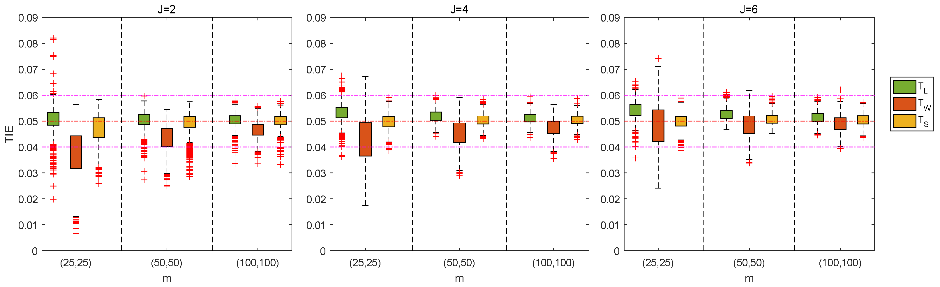
The performance of the proposed testing methods is assessed by examining empirical type I error rates (TIEs) and empirical powers. In the simulation studies, all tests are conducted at the significance level α = 0.05 . 10,000 samples are randomly generated under the null hypothesis, and empirical type I error rates are computed by dividing the number of times the null hypothesis is rejected by 10,000. According to Tang et al. [26], a test is liberal if its empirical TIEs are greater than 0.06, conservative if the TIEs are less than 0.04, and otherwise robust. The results for J = 4 are shown in Table 3, while those for J = 2 and J = 6 are provided in Supplementary Material S1. The findings indicate that tests based on larger sample sizes perform more satisfactorily than those based on smaller sample sizes, across a range of parameter configurations. T W tends to be more conservative in the small sample size m = ( 25 , 25 ) , ( 50 , 50 ) . And T L is more liberal for the m = ( 25 , 25 ) . T S behaves satisfactorily, in the sense that its type I error rate is close to the pre-determined nominal level of 0.05 for any configuration. A total of 1000 parameter configurations are randomly generated to evaluate the test statistics, with empirical TIEs visualized using box plots in Figure 1. The results indicate that T L tends to be increasingly liberal as the number of strata grows, while T W is even more affected, although its performance improves with larger sample sizes and more strata. Notably, T S demonstrates superior robustness across all settings and is thus recommended for testing homogeneity.
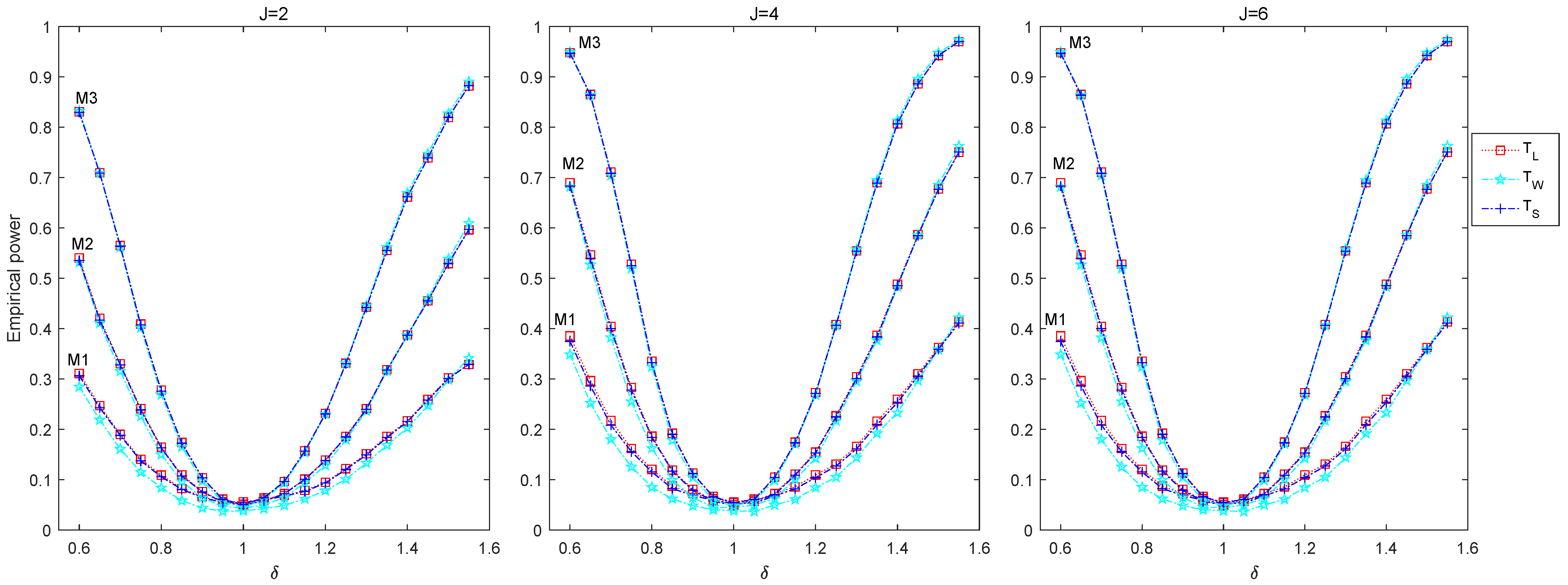
Then, the performance of powers is investigated for the proposed test statistics under the same parameter configurations (Table 2). In the simulation studies, the data are generated under the alternative hypothesis. The empirical power is calculated as the proportion of correct rejections of the null hypothesis in 10,000 Monte Carlo repetitions. Empirical power results for J = 4 are presented in Table 4 and Supplementary Material S2. The powers of all three test statistics increase with larger sample sizes and more strata. For δ 1 and δ 2 , the powers of T L and T S are greater than that of T W . However, the opposite conclusion will be reached for δ 3 . Furthermore, Figure 2 further shows the relationship between the power and parameter δ in the alternative hypotheses. Suppose that δ = 0.6 ( 0.05 ) 1.55 , i.e., from 0.6 to 1.55 with step size 0.05. Other parameter configurations are set in case III, a2 and b2 (Table 2) for strata J = 2 , 4 , 6 and group number M1 = (25, 25), M2 = (50, 50), M3 = (100, 100). The results reflect that the power is greatly influenced by δ . Interestingly, the closer the alternative hypothesis is to the null hypothesis, the lower the power. Moreover, the power of T W is significantly smaller than the power of T L and T S with δ ( 0.6 , 1.45 ) and M1.

4.2. The Performance of Sample Size Determination

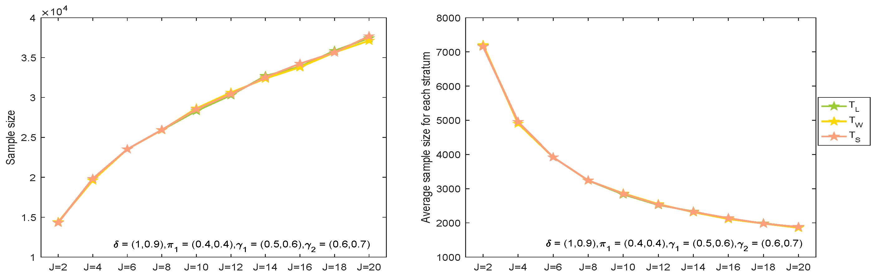
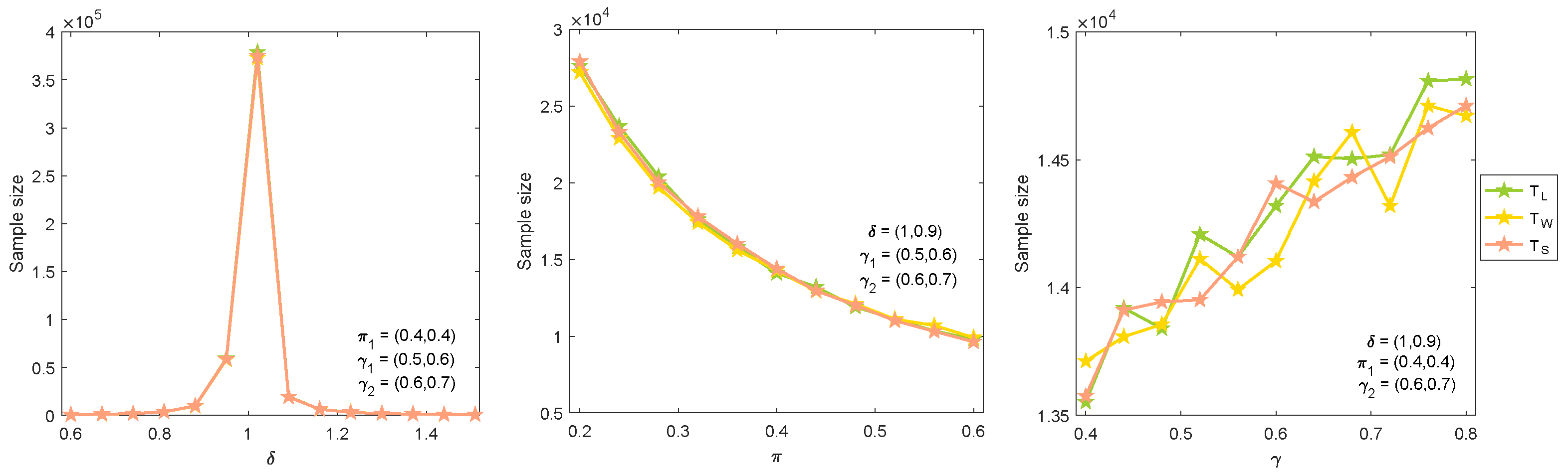
The sample size determination methods are evaluated based on their empirical powers. In the simulation studies, the same parameter settings of δ , π 1 and γ i ( i = 1 , 2 ) are selected as in Table 2 for the stratum J = 2 , 4 , 6 . For any given parameters, the sample size and estimated power are computed iteratively at α = 0.05 for target powers of 80 % or 90 % . Results for target powers of 80 % and 90 % are presented in Table 5 and Table 6. The estimated powers fluctuate around the desired levels. As expected, the required sample size for 90 % power is substantially larger than that for 80 % power. Sample sizes increase with both the stratum size (i.e., the number of subjects per stratum) and the number of strata. They also vary across different parameter configurations. Figure 3 and Figure 4 further illustrate the relationship between sample size and these factors. As the number of strata J increases from 2 to 20, the total sample size increases while the average sample size per stratum decreases. In Figure 4, with π 1 = ( 0.4 , π ) and γ 1 = ( 0.5 , γ ) , we observe that the sample size is more sensitive to changes in δ and π 1 j than to those in γ 1 j . And the sample size becomes larger when δ is closer to 1. This conclusion coincides with the result of the correlation between power and δ in Section 4.1. Moreover, the sample size decreases as π increases, which is because the change in π will affect the value of δ .

5. Two Real Examples

To address the unilateral and bilateral combined data structure, two real examples of otolaryngology and myopathy provide us with the ability to implement our methodology for real-world data. For the otolaryngology study (Table 5 of Reference [20]), the risk ratio is δ j = π 2 j / π 1 j ( j = 1 , 2 , 3 ) . The homogeneity hypothesis H 0 : δ 1 = δ 2 = δ 3 δ versus H 1 : δ r δ s ( r s ) is tested to determine whether children of different ages require distinct antibiotics for improved treatment outcomes. The unconstrained MLEs are δ ^ = ( 2.1749 , 1.5609 , 0.9503 ) , π ^ 1 = ( 0.1871 , 0.4375 , 0.6803 ) , γ ^ 1 = ( 0.6553 , 0.8790 , 0.9878 ) and γ ^ 2 = ( 0.8688 , 0.8199 , 0.7633 ) . The results of the constrained MLEs can be found in Table 6 of Reference [20].
Table 7 presents the corresponding statistical values and p-values based on the three proposed tests for two examples. The results show that all p-values are above 0.05 under H 0 , failing to reject the null hypothesis of no treatment difference in relative risk ratio across the three age strata between Cefaclor and Amoxicillin.
The parameter estimates are identical to the MLEs given above. Table 8 reports the sample sizes and corresponding estimated powers under target powers of 80 % and 90 % at α = 0.05 . The sample sizes for the three tests are generally accurate, with empirical powers close to the pre-specified levels, and are thus recommended for this example. While T W requires a smaller sample size than T L and T S , T S yields estimated powers closer to the nominal values. Consequently, to achieve 80 % (or 90 % ) power, sample sizes of 504 (or 756) are needed.
Another example is a recorded observational study on myopia patients (Table 9 of Reference [20]). We are interested in comparing the effectiveness of treatments between the VST and CRT groups across genders. Apply the proposed methods to test H 0 : δ 1 = δ 2 δ vs. H 1 : δ r δ s ( r s ; s , r { 1 , 2 } ) . According to the calculation, the unconstrained MLEs are δ ^ = ( δ ^ 1 , δ ^ 2 ) = ( 0.0737 , 0.9467 ) , π ^ 1 = ( 0.4340 , 0.3201 ) , γ ^ 1 = ( 0.8189 , 0.6354 ) and γ ^ 2 = ( 0.7282 , 0.6688 ) . Table 8 indicates that T L and T S have greater estimated power than T W . In order to obtain more robust results and the desired power to reach 80% (or 90%), 120 (or 160) samples are needed.

6. Conclusions

We develop three asymptotic tests and three iterative sample size determination methods for the risk ratio based on stratified unilateral and bilateral data within Dallal’s model. The unconstrained and constrained MLEs are derived using the Newton–Raphson procedure and the Fisher scoring algorithm. Simulation results support the recommendation of the score test for evaluating treatment effectiveness under a variety of data-generating scenarios. The sample size methods based on the score test or the likelihood ratio test are also suggested for determining the empirical sample size, because their estimated powers are closer to empirical powers than those based on the Wald-type test. Furthermore, two real-world datasets of acute otitis media and myopic eyes are used to illustrate the application of the proposed tests and sample size determination.
The contributions of this work extend beyond the following: (i) Many current studies tend to analyze bilateral data without considering unilateral data. However, the unilateral data is also obtained in clinical practice, when only one side of the patient’s paired organs is diseased or has received treatment. Our methodologies can be applied not only to the research of bilateral data, but also to the research of unidirectional and bilateral data. In our context, the scenario of bilateral data alone constitutes a special case. (ii) In practice, sample size is one of the essential factors in designing clinical accuracy trials. Through the study of sample size, the statistical test can achieve a specified power at a given nominal level in all paired medical trials. In actual data research, it will lead to inaccurate test results if the sample size is insufficient. When the sample size is too large, it will lead to unnecessary waste of resources. Therefore, the sample size determination is discussed based on the stratified unilateral and bilateral data in this paper.
Despite its satisfactory performance, the proposed method has two limitations. First, the iterative sample size determination process is computationally intensive. Second, the reliability of the method relies on the assumption of large stratum sizes, and its performance in sparse data settings requires further investigation. Therefore, future research should focus on developing exact methods for small-sample data to enhance its applicability.


Supplementary Materials

The following supporting information can be downloaded at: https://www.mdpi.com/article/10.3390/axioms15040268/s1, Table S1: The empirical TIEs (%) for J = 2. Table S2: The empirical TIEs (%) for J = 6. Table S3: The empirical powers (%) for J = 2. Table S4: The empirical powers (%) for J = 6.

Author Contributions

Conceptualization, investigation, project administration, writing—original draft, S.S.; Writing—review and editing, supervision, Z.L. All authors have read and agreed to the published version of the manuscript.

Funding

The work was supported by the Natural Science Research Start-up Foundation of Recruiting Talents of Nanjing University of Posts and Telecommunications (XK0070922093), the Central Guidance for Local Science and Technology Development Fund (ZYYD2025ZY20), the National Natural Science Foundation of China (12561047), and the Xinjiang Talent Development Fund (XJRC-2025-KJ-PY-KJLJ-108).

Institutional Review Board Statement

Not applicable.

Informed Consent Statement

Not applicable.

Data Availability Statement

The data presented in this study are openly available in [Pediatr. Infect. Dis. J.] at [DOI: https://doi.org/10.1097/00006454-198209000-00006] and in [Stat. Pap.] at [DOI: https://doi.org/10.1007/s00362-024-01532-6].

Conflicts of Interest

The authors declare no conflicts of interest.

Appendix A

Appendix A.1. Information Matrix for Computing MLEs

The Fisher information matrix I 1 is given by:
I 1 ( π i j , γ i j ) = E 2 l 1 π i j 2 E 2 l 1 π i j γ i j E 2 l 1 π i j γ i j E 2 l 1 γ i j 2 ,
and
E 2 l 1 π i j 2 = m i j ( 1 ) π i j 1 + m i j ( 1 ) m i j ( 2 ) ( γ i j 2 ) π i j + m i j ( 2 ) ( γ i j 2 ) 2 π i j ( γ i j 2 ) + 1 , E 2 l 1 γ i j 2 = m i j ( 2 ) π i j γ i j 2 m i j ( 2 ) π i j γ i j 1 + m i j ( 2 ) π i j 2 π i j ( γ i j 2 ) + 1 , E 2 l 1 π i j γ i j = m i j ( 2 ) π i j ( γ i j 2 ) + 1 .
Differentiating the log-likelihood function (3) with δ , π 1 j , γ 1 j , and γ 2 j are as follows:
l 0 δ = j = 1 J m 12 j ( 1 ) + m 12 j ( 2 ) + m 22 j ( 2 ) δ + m 02 j ( 1 ) π 1 j π 1 j δ 1 + m 02 j ( 2 ) π 1 j ( γ 2 j 2 ) π 1 j δ ( γ 2 j 2 ) + 1 , 2 l 0 δ 2 = j = 1 J m 12 j ( 1 ) + m 12 j ( 2 ) + m 22 j ( 2 ) δ 2 + m 02 j ( 1 ) π 1 j 2 ( π 1 j δ 1 ) 2 + m 02 j ( 2 ) π 1 j 2 ( γ 2 j 2 ) 2 ( π 1 j δ ( γ 2 j 2 ) + 1 ) 2 , l 0 π 1 j = m 1 + j ( 1 ) + m 1 + j ( 2 ) + m 2 + j ( 2 ) π 1 j + m 01 j ( 1 ) π 1 j 1 + m 02 j ( 1 ) δ π 1 j δ 1 + m 01 j ( 2 ) ( γ 1 j 2 ) π 1 j ( γ 1 j 2 ) + 1 + m 02 j ( 2 ) δ ( γ 2 j 2 ) π 1 j δ ( γ 2 j 2 ) + 1 , l 0 γ 1 j = m 21 j ( 2 ) γ 1 j + m 11 j ( 2 ) γ 1 j 1 + m 01 j ( 2 ) π 1 j π 1 j ( γ 1 j 2 ) + 1 , l 0 γ 2 j = m 22 j ( 2 ) γ 2 j + m 12 j ( 2 ) γ 2 j 1 + m 02 j ( 2 ) π 1 j δ π 1 j δ ( γ 2 j 2 ) + 1 .
The Fisher information matrix I 0 is written as follows:
I 0 ( π 1 j , γ 1 j , γ 2 j ) = I 11 j I 12 j I 13 j I 21 j I 22 j I 23 j I 13 j I 23 j I 33 j ,
where
I 11 j = E 2 l 0 π 1 j 2 = m + 1 j ( 1 ) + m + 2 j ( 1 ) δ m + 1 j ( 2 ) ( γ 1 j 2 ) m + 2 j ( 2 ) ( γ 2 j 2 ) δ π 1 j m + 1 j ( 1 ) π 1 j 1 m + 2 j ( 1 ) δ 2 π 1 j δ 1 + m + 1 j ( 2 ) ( γ 1 j 2 ) 2 π 1 j ( γ 1 j 2 ) + 1 + m + 2 j ( 2 ) ( γ 2 j 2 ) 2 δ 2 π 1 j ( γ 2 j 2 ) δ + 1 , I 12 j = E 2 l 0 π 1 j γ 1 j = m + 1 j ( 2 ) π 1 j ( γ 1 j 2 ) + 1 , I 13 j = E 2 l 0 π 1 j γ 2 j = m + 2 j ( 2 ) δ π 1 j ( γ 2 j 2 ) δ + 1 , I 22 j = E 2 l 0 γ 1 j 2 = m + 1 j ( 2 ) π 1 j γ 1 j 2 m + 1 j ( 2 ) π 1 j γ 1 j 1 + m + 1 j ( 2 ) π 1 j 2 π 1 j ( γ 1 j 2 ) + 1 , I 23 j = E 2 l 0 γ 1 j γ 2 j = 0 , I 33 j = E 2 l 0 γ 2 j 2 = m + 2 j ( 2 ) π 1 j δ γ 2 j 2 m + 2 j ( 2 ) π 1 j 2 δ 2 γ 2 j 1 + m + 2 j ( 2 ) π 1 j 2 π 1 j ( γ 2 j 2 ) δ + 1 .

Appendix A.2. Derivation of Wald-Type Test

The Wald test statistic for H 0 : δ 1 = = δ J is:
T W = p = 1 J 1 q = 1 J 1 ( δ ^ p δ ^ p + 1 ) ( δ ^ q δ ^ q + 1 ) E p , q 1 ( δ ^ ) ,
where E p , q 1 ( δ ^ ) denotes the ( p , q ) -th element of the inverse of the covariance matrix of the successive differences δ ^ p δ ^ p + 1 ( p = 1 , , J 1 ). To derive its explicit form, we assume that δ ^ 1 , , δ ^ J are independent and denote their variances by e 1 , , e J ( e j > 0 ). Under this assumption, the covariance matrix V of ( δ ^ 1 δ ^ 2 , , δ ^ J 1 δ ^ J ) takes the following symmetric tridiagonal form:
V = e 1 + e 2 e 2 0 0 e 2 e 2 + e 3 e 3 0 0 e 3 e 3 + e 4 0 0 0 0 e J 1 e J 1 + e J .
To derive the explicit form of its inverse, we introduce the following notation. For positive quantities e 1 , , e J , define C { a 1 , , a m } 1 = i = 1 m j i a j (the sum of all products obtained by deleting one element), with the convention C { a 1 } 1 = 1 . Also define e p , q = k = p + 1 q e k for p < q , and e p , p = 1 .
The determinant of V can be computed via the standard recurrence for tridiagonal matrices and simplifies to:
det ( V ) = C { e 1 , , e J } 1 .
For 1 p , q J 1 , let V ( q , p ) be the matrix obtained from V by deleting the q-th row and the p-th column. By exploiting the tridiagonal structure, one finds that for p q ,
det ( V ( q , p ) ) = ( 1 ) p + q e p , q C { e 1 , , e p } 1 C { e q + 1 , , e J } 1 ,
and the case p > q follows by symmetry. The inverse elements are given by ( V 1 ) p q = ( 1 ) p + q det ( V ( q , p ) ) / det ( V ) . For all p , q , substituting the expressions above yields:
( V 1 ) p q = C { e 1 , , e min ( p , q ) } 1 C { e max ( p , q ) + 1 , , e J } 1 e min ( p , q ) , max ( p , q ) C { e 1 , , e J } 1 .
Evaluating this at the estimated values δ ^ (which determine the e i ) gives E p , q 1 ( δ ^ ) as stated in the main text.

Appendix A.3. Derivation of Score Statistic

The Fisher information matrix I ( θ ) is:
I ( θ ) = I δ δ I δ π 1 I δ γ I π 1 δ I π 1 π 1 I π 1 γ I γ δ I γ π 1 I γ γ ,
where
I δ δ = E 2 l 0 δ δ T , I δ π 1 = I π 1 δ T = E 2 l 0 δ π 1 T , I δ γ = I γ δ T = E 2 l 0 δ γ T , I π 1 π 1 = E 2 l 0 π 1 π 1 T , I π 1 γ = I γ π 1 T = E 2 l 0 π 1 γ T , I γ γ = E 2 l 0 γ γ T ,
and
E ( 2 l 0 δ π 1 j ) = m + 2 j ( 1 ) π 1 j δ 1 m + 2 j ( 2 ) ( γ 2 j 2 ) π 1 j δ ( γ 2 j 2 ) + 1 , E ( 2 l 0 δ γ 1 j ) = 0 , E ( 2 l 0 δ γ 2 j ) = m + 2 j ( 2 ) π 1 j π 1 j δ ( γ 2 j 2 ) + 1 .

References

  1. Gu, J.X.; Chen, Q.; Zhang, P.J.; Zhang, T.; Zhou, X.; Zhang, K.; Jiang, T.; Liu, S.; Chen, W.; Zhou, M.; et al. Characteristics of vitreoretinal lymphoma in B-scan ultrasonography: A case-control study. Ophthalmol. Retin. 2024, 8, 264–269. [Google Scholar]
  2. Bomdica, P.R.; MacCumber, M.; Abdel-Hadi, S.; Parker, M.; Minaker, S. Surgical outcomes of rhegmatogenous retinal detachment and fellow eye involvement in adolescent and young adult patients. Ophthalmol. Retin. 2024, 8, 148–154. [Google Scholar] [CrossRef] [PubMed]
  3. Zhang, H.G.; Ying, G.S. Statistical approaches in published ophthalmic clinical science papers: A comparison to statistical practice two decades ago. Brit. J. Ophthalmol. 2018, 102, 1188–1191. [Google Scholar] [CrossRef]
  4. Rosner, B. Statistical methods in ophthalmology: An adjustment for the intraclass correlation between eyes. Biometrics 1982, 38, 105–114. [Google Scholar] [CrossRef]
  5. Dallal, G.E. Paired Bernoulli trials. Biometrics 1988, 44, 253–257. [Google Scholar] [CrossRef]
  6. Donner, A. Statistical methods in opthalmology: An adjusted chi-square approach. Biometrics 1989, 45, 605–611. [Google Scholar] [CrossRef]
  7. Tang, N.S.; Tang, M.L.; Qiu, S.F. Testing the equality of proportions for correlated otolaryngologic data. Comput. Stat. Data Anal. 2008, 52, 3719–3729. [Google Scholar] [CrossRef]
  8. Pei, Y.B.; Tian, G.L.; Tang, M.L. Testing homogeneity of proportion ratios for stratified correlated bilateral data in two arm randomized clinical trials. Stat. Med. 2014, 33, 4370–4386. [Google Scholar] [CrossRef]
  9. Zhuang, T.T.; Tian, G.L.; Ma, C.X. Homogeneity test of ratio of two proportions in stratified bilateral data. Stat. Biopharm. Res. 2019, 11, 200–209. [Google Scholar] [CrossRef]
  10. Tang, N.S.; Qiu, S.F.; Tang, M.L.; Pei, Y.B. Asymptotic confidence interval construction for proportion difference in medical studies with bilateral data. Stat. Methods Med. Res. 2011, 20, 233–259. [Google Scholar] [CrossRef]
  11. Pei, Y.B.; Tang, M.L.; Wong, W.K.; Guo, J.H. Confidence intervals for correlated proportion differences from paired data in a two-arm randomised clinical trial. Stat. Methods Med. Res. 2012, 21, 167–187. [Google Scholar] [CrossRef]
  12. Shen, X.; Ma, C.X.; Yuen, K.C.; Tian, G.L. Common risk difference test and interval estimation of risk difference for stratified bilateral correlated data. Stat. Methods Med. Res. 2018, 28, 2418–2438. [Google Scholar] [CrossRef]
  13. Mandel, E.M.; Bluestone, C.D.; Rockette, H.E.; Blatter, M.M.; Reisinger, K.S.; Wucher, F.P.; Harper, J. Duration of effusion after antibiotic treatment for acute otitis media: Comparison of Cefaclor and Amoxicillin. Pediatr. Infect. Dis. 1982, 1, 310–316. [Google Scholar] [CrossRef]
  14. Liang, S.Y.; Fang, K.T.; Huang, X.W.; Xin, Y.; Ma, C.X. Homogeneity tests and interval estimations of risk differences for stratified bilateral and unilateral correlated data. Stat. Pap. 2024, 65, 3499–3543. [Google Scholar] [CrossRef]
  15. Wang, H.P.; Ma, C.X. Homogeneity test of ratios of two proportions in stratified bilateral and unilateral data. Mathematics 2024, 12, 2719. [Google Scholar] [CrossRef]
  16. Hua, S.C.; Ma, C.X. Testing the homogeneity of odds ratio across strata for combined bilateral and unilateral data. PloS One 2024, 19, e0307276. [Google Scholar] [CrossRef]
  17. Hua, S.C.; Ma, C.X. Common odds ratio test and interval estimation for stratified bilateral and unilateral data. Stat. Methods Med. Res. 2024, 33, 1559–1576. [Google Scholar] [CrossRef]
  18. Sun, S.M.; Li, Z.M.; Mou, K.Y. Interval estimation of common risk difference for stratified unilateral and bilateral data. J. Biopharm. Stat. 2024, 35, 85–105. [Google Scholar] [CrossRef] [PubMed]
  19. Sun, S.M.; Li, Z.M.; Jiang, H.J. Homogeneity test and sample size of risk difference for stratified unilateral and bilateral data. Commun. Stat. Simul. C 2024, 53, 4209–4232. [Google Scholar] [CrossRef]
  20. Sun, S.M.; Li, Z.M. Common test and interval estimation of risk ratio for complex paired data under Dallal’s model. Mathematics 2026, 14, 948. [Google Scholar] [CrossRef]
  21. Sun, S.M.; Li, Z.M.; Ai, M.Y.; Jiang, H.J. Risk difference tests for stratified binary data under Dallal’s model. Stat. Methods Med. Res. 2022, 31, 1135–1156. [Google Scholar] [CrossRef]
  22. Maria, S.; Antonia, Z. Sample size calculation and re-estimation based on the prevalence in a single-arm confirmatory diagnostic accuracy study. Stat. Methods Med. Res. 2020, 29, 2958–2971. [Google Scholar]
  23. Qiu, S.F.; Fu, Q.X. Homogeneity testing for binomial proportions under stratified double-sampling scheme with two fallible classifiers. Stat. Methods Med. Res. 2020, 29, 3547–3568. [Google Scholar] [CrossRef] [PubMed]
  24. Mou, K.Y.; Li, Z.M.; Ma, C.X. Asymptotic sample size for common test of relative risk ratios in stratified bilateral data. Mathematics 2023, 11, 4198. [Google Scholar] [CrossRef]
  25. Sampson, J.N.; Gail, M.H. Confidence intervals for the difference between two relative risks. Stat. Methods Med. Res. 2020, 29, 3048–3058. [Google Scholar] [CrossRef]
  26. Tang, N.S.; Qiu, S.F. Homogeneity test, sample size determination and interval construction of difference of two proportions in stratified bilateral-sample designs. J. Stat. Plan Inference 2012, 142, 1243–1251. [Google Scholar] [CrossRef]
Figure 1. Box-plots of empirical TIEs for the likelihood ratio test ( T L ), Wald-type test ( T W ), and score test ( T S ) when J = 2 , 4 , 6 and m = ( 25 , 25 ) , ( 50 , 50 ) , ( 100 , 100 ) .
Axioms 15 00268 g001
Figure 2. The curve graph of empirical powers for δ under the parameter settings III, a2 and b2. The quantities for each group are selected as M1 = (25, 25), M2 = (50, 50), and M3 = (100, 100).
Axioms 15 00268 g002
Figure 3. The estimated sample size with each stratum for the desired power 80%.
Axioms 15 00268 g003
Figure 4. The estimated sample size with three parameters δ , π and γ for the desired power 80%.
Axioms 15 00268 g004
Table 1. Data structure of the jth stratum.
Number of ResponsesGroup (i)Total
12
0 m 01 j ( 1 ) ( p 01 j ( 1 ) ) m 02 j ( 1 ) ( p 02 j ( 1 ) ) m 0 + j ( 1 )
1 m 11 j ( 1 ) ( p 11 j ( 1 ) ) m 12 j ( 1 ) ( p 12 j ( 1 ) ) m 1 + j ( 1 )
Total m 1 j ( 1 ) m 2 j ( 1 ) N j
0 m 01 j ( 2 ) ( p 01 j ( 2 ) ) m 02 j ( 2 ) ( p 02 j ( 2 ) ) m 0 + j ( 2 )
1 m 11 j ( 2 ) ( p 11 j ( 2 ) ) m 12 j ( 2 ) ( p 12 j ( 2 ) ) m 1 + j ( 2 )
2 m 21 j ( 2 ) ( p 21 j ( 2 ) ) m 22 j ( 2 ) ( p 22 j ( 2 ) ) m 2 + j ( 2 )
Total m 1 j ( 2 ) m 2 j ( 2 ) N j
Table 2. The parameter configuration.
ParameterCasesNumber of Strata
J = 2 J = 4 J = 6
π 1 I(0.3,0.5)(0.3,0.5,0.3,0.5)(0.3,0.5,0.3,0.5,0.3,0.5)
II(0.4,0.5)(0.4,0.5,0.4,0.5)(0.4,0.5,0.4,0.5,0.4,0.5)
III(0.4,0.4)(0.4,0.4,0.4,0.4)(0.4,0.4,0.4,0.4,0.4,0.4)
γ 1 a1(0.5,0.5)(0.5,0.5,0.5,0.5)(0.5,0.5,0.5,0.5,0.5,0.5)
a2(0.5,0.6)(0.5,0.6,0.5,0.6)(0.5,0.6,0.5,0.6,0.5,0.6)
γ 2 b1(0.5,0.6)(0.5,0.6,0.5,0.6)(0.5,0.6,0.5,0.6,0.5,0.6)
b2(0.6,0.7)(0.6,0.7,0.6,0.7)(0.6,0.7,0.6,0.7,0.6,0.7)
Table 3. The empirical TIEs (%) of T L , T W , T S for J = 4 .
δ π 1 γ 1 γ 2 m = ( 25 , 25 ) m = ( 50 , 50 ) m = ( 100 , 100 )
T L T W T S T L T W T S T L T W T S
0.7Ia1b15.224.724.885.475.215.305.065.114.94
b25.515.305.185.165.134.914.964.784.88
a2b15.444.705.055.194.875.104.884.704.80
b25.354.885.005.475.355.325.264.985.16
IIa1b15.334.474.864.824.554.755.655.335.55
b25.524.825.335.064.864.915.505.235.40
a2b15.884.715.625.054.584.914.774.574.73
b25.364.595.015.044.434.915.164.755.08
0.9Ia1b15.735.015.375.335.135.205.304.805.18
b25.324.474.995.044.694.945.285.035.23
a2b15.584.685.295.504.875.314.884.504.81
b25.524.715.215.395.095.235.064.714.94
IIa1b15.774.615.555.324.745.155.335.085.28
b25.434.655.134.944.194.795.044.724.94
a2b15.514.145.125.114.265.005.414.995.30
b25.234.175.025.294.575.145.355.085.32
1.2Ia1b14.924.064.464.954.234.784.744.414.70
b25.454.265.185.334.635.214.834.554.74
a2b14.964.314.675.824.885.654.994.664.87
b25.594.075.314.833.994.614.954.534.86
IIa1b15.143.914.775.214.185.005.074.444.94
b25.623.955.325.224.575.004.834.554.74
a2b15.493.805.264.773.984.655.254.635.21
b25.663.935.205.064.244.965.134.635.08
Table 4. The empirical powers (%) for J = 4 .
δ π 1 γ 1 γ 2 m = ( 25 , 25 ) m = ( 50 , 50 ) m = ( 100 , 100 )
T L T W T S T L T W T S T L T W T S
δ 1 Ia1b121.449.9220.8539.4526.5039.2070.9862.6070.94
b221.059.2720.5237.5826.3537.5469.1061.1369.14
a2b121.039.8720.5339.2527.5639.1269.1962.0369.19
b220.839.7420.6137.9126.3937.8668.0760.5768.10
IIa1b127.8120.7326.7350.3145.1749.7883.4881.7983.42
b227.6520.7727.0548.6743.6448.3681.0479.0380.92
a2b127.5520.4126.7750.6745.9750.1982.4680.8282.33
b226.6020.4126.0148.6544.1048.1880.1378.1879.93
δ 2 Ia1b16.773.526.358.434.918.2210.707.2310.55
b26.693.716.437.564.247.4210.477.1610.48
a2b16.703.386.427.905.047.8210.597.5010.49
b26.333.656.037.824.537.7310.807.5910.76
IIa1b17.514.577.148.866.398.6413.0010.5812.86
b27.374.846.998.416.378.2912.5410.7312.44
a2b17.574.797.238.266.578.1412.6710.7312.49
b27.094.376.748.516.518.3612.5210.5912.33
δ 3 Ia1b19.5513.339.3314.6219.7014.4925.8531.3525.84
b210.0913.249.6114.5819.1214.3825.2030.6625.18
a2b19.0212.348.6514.6818.7114.5425.7930.5725.74
b29.5813.039.1714.0817.9713.8824.4829.3524.38
IIa1b112.1013.2011.6619.6721.7819.4836.0639.3436.00
b211.3712.5710.9019.3921.1619.1834.6637.6534.46
a2b111.9412.3111.5818.7420.4518.4135.3837.5735.23
b211.5412.1911.1018.6820.0818.3933.5436.1433.44
Note: δ 1 = (1,0.7); δ 2 = (1,0.9); and δ 3 = (1,1.2). T L , T W , and T S respectively represent three tests, corresponding to their empirical powers.
Table 5. Sample size (estimated powers %) for the homogeneity test with 80% power.
δ π 1 γ 1 γ 2 J = 2 J = 4 J = 6
T L T W T S T L T W T S T L T W T S
δ 1 Ia1b11424(79.78)1536(79.71)1416(79.97)1984(79.66)2192(80.00)1984(79.48)2328(79.82)2664(79.75)2352(80.00)
b21488(79.81)1592(79.53)1472(79.67)2080(79.97)2288(79.76)2064(79.82)2424(79.90)2760(79.84)2424(80.03)
a2b11448(79.78)1544(80.10)1440(79.76)2000(79.74)2224(79.93)2000(79.46)2352(79.22)2688(79.99)2400(80.17)
b21512(79.89)1608(79.45)1512(79.87)2112(80.08)2304(79.83)2096(80.06)2448(79.98)2808(79.99)2448(80.18)
IIa1b11064(80.22)1096(79.80)1072(79.88)1472(79.60)1552(80.14)1488(80.25)1728(79.62)1872(80.00)1728(79.41)
b21128(79.95)1144(79.82)1112(79.64)1552(80.16)1632(79.99)1520(79.48)1824(80.43)1944(79.99)1824(79.95)
a2b11088(80.01)1112(80.08)1072(79.73)1520(79.71)1552(79.64)1536(80.00)1776(79.77)1872(80.27)1800(79.85)
b21144(80.19)1168(80.13)1136(79.96)1568(80.09)1648(80.37)1584(79.57)1848(79.95)1944(80.00)1848(79.40)
δ 2 Ia1b114,920(80.04)15,408(79.79)14,912(79.88)20,560(79.96)21,424(80.03)20,816(79.64)24,336(79.95)25,440(79.81)24,432(79.61)
b215,424(79.76)15,712(79.92)15,512(79.96)21,440(80.29)22,304(79.53)21,344(79.40)25,008(79.77)26,232(79.93)24,936(79.26)
a2b115,024(79.95)15,608(79.99)15,136(79.93)21,232(80.52)21,808(79.87)21,024(79.79)24,816(79.92)25,728(79.75)24,624(79.99)
b215,920(79.85)15,912(79.68)15,720(80.24)21,840(79.56)22,800(79.54)21,824(79.98)25,824(79.90)26,640(79.81)25,728(80.05)
IIa1b110,720(80.18)10,920(79.70)10,848(79.76)14,880(79.69)15,408(79.73)14,944(80.50)17,808(79.77)18,288(79.68)17,712(79.92)
b211,224(80.11)11,504(80.13)11,312(79.68)15,712(79.99)16,016(79.96)15,632(80.20)18,552(79.84)18,816(80.31)18,528(79.70)
a2b110,944(79.78)11,216(80.18)11,120(79.87)15,328(80.28)15,632(80.29)15,408(79.80)18,216(79.67)18,408(79.81)18,120(80.11)
b211,528(79.81)11,648(79.67)11,520(79.92)16,128(79.96)16,208(79.92)16,112(79.77)18,840(79.84)19,320(79.97)18,936(79.91)
δ 3 Ia1b14512(79.81)4264(79.74)4480(79.75)6256(79.90)5808(79.76)6224(79.97)7272(80.11)6720(80.20)7344(79.85)
b24624(79.90)4448(79.74)4712(79.49)6496(79.99)6032(80.61)6432(80.11)7632(80.10)7008(79.91)7632(80.35)
a2b14608(79.66)4384(79.78)4608(79.97)6320(79.73)5936(79.99)6320(79.94)7440(79.88)6936(80.03)7392(79.92)
b24712(79.93)4528(80.23)4808(80.09)6624(79.70)6144(80.36)6528(79.82)7680(79.43)7128(79.81)7656(79.94)
IIa1b13112(80.08)3032(79.86)3136(79.80)4320(79.45)4208(80.03)4400(80.41)5136(80.00)4848(79.78)5208(79.80)
b23264(79.79)3224(79.80)3280(79.95)4544(80.14)4352(79.25)4560(80.05)5328(79.95)5088(80.29)5424(79.84)
a2b13216(79.88)3072(79.17)3224(79.95)4448(80.19)4352(80.38)4496(79.96)5232(80.32)5040(79.90)5256(80.19)
b23408(79.99)3320(79.95)3352(79.76)4656(79.89)4480(79.73)4624(79.16)5520(80.51)5280(80.14)5448(79.93)
Note: δ 1 = (1,0.7); δ 2 = (1,0.9); δ 3 = (1,1.2).
Table 6. Sample size (estimated powers %) for the homogeneity test with 90% power.
δ π 1 γ 1 γ 2 J = 2 J = 4 J = 6
T L T W T S T L T W T S T L T W T S
δ 1 Ia1b11912(89.76)2016(90.08)1928(89.88)2608(89.93)2816(90.14)2560(89.49)2976(89.98)3336(89.92)3000(89.89)
b21992(90.00)2064(89.62)1984(89.99)2672(89.65)2896(89.74)2704(89.92)3120(89.98)3432(90.19)3120(89.87)
a2b11928(89.89)2048(89.89)1912(89.72)2624(89.96)2816(89.73)2624(90.11)3048(89.90)3312(89.84)3024(90.04)
b22016(89.76)2120(89.87)2024(89.75)2720(90.00)2912(89.91)2704(89.72)3192(89.87)3480(89.95)3144(90.25)
IIa1b11416(89.71)1456(89.90)1432(89.87)1904(89.63)1968(89.60)1920(89.93)2232(89.88)2352(90.09)2256(89.73)
b21512(89.91)1520(89.93)1480(89.94)2016(90.07)2096(89.87)2032(89.98)2328(89.92)2448(89.85)2352(90.08)
a2b11464(89.81)1480(89.85)1464(89.96)1952(90.05)1984(89.24)1968(89.82)2280(90.15)2352(89.92)2280(89.92)
b21520(89.74)1552(90.22)1520(90.07)2048(89.95)2128(89.78)2064(89.91)2376(89.95)2496(90.04)2400(89.95)
δ 2 Ia1b119,712(89.95)20,040(89.99)20,024(90.03)26,944(89.87)27,808(90.18)26,784(89.66)31,512(89.88)32,016(89.82)31,416(89.90)
b220,816(89.95)20,904(89.95)20,824(89.95)27,920(89.69)28,800(89.86)27,920(89.90)32,424(90.19)33,432(89.90)32,520(89.81)
a2b120,312(89.57)20,536(89.91)20,216(89.98)27,232(89.93)28,000(89.90)27,408(89.74)31,728(89.76)32,832(89.86)31,920(89.54)
b221,016(89.99)21,152(89.69)21,112(89.98)28,416(89.97)28,912(90.34)28,320(89.99)32,832(89.79)33,864(89.66)32,928(89.98)
IIa1b114,336(89.50)14,608(90.12)14,512(90.10)19,888(89.83)19,808(90.05)19,712(89.72)22,536(89.77)22,896(90.13)22,752(90.29)
b215,120(89.97)15,136(89.91)15,208(89.92)20,624(89.95)20,832(89.91)20,320(89.93)23,904(89.77)23,952(89.94)23,928(89.63)
a2b114,752(89.71)14,944(89.76)14,840(89.91)19,920(89.57)20,320(89.86)19,920(89.86)23,424(89.95)23,520(90.22)23,232(89.76)
b215,416(89.77)15,616(89.94)15,432(89.83)21,088(89.91)21,120(90.27)20,912(89.82)24,240(89.92)24,720(89.89)24,312(90.00)
δ 3 Ia1b16016(90.14)5760(89.57)6024(89.96)8080(89.92)7712(89.92)8112(89.81)9432(90.08)8832(89.84)9432(89.80)
b26312(89.89)6008(89.72)6304(89.89)8512(90.17)7984(90.31)8432(89.99)9720(89.71)9144(89.50)9792(90.10)
a2b16120(89.98)6000(89.96)6112(90.24)8320(89.82)7824(89.93)8320(90.00)9648(89.90)8976(89.83)9528(90.00)
b26360(89.94)6096(89.58)6336(89.93)8624(89.99)8112(89.52)8624(90.08)9864(89.86)9312(89.85)9912(89.55)
IIa1b14232(89.84)4064(89.76)4136(89.93)5712(89.85)5520(89.98)5568(89.82)6624(89.98)6240(89.70)6552(89.90)
b24360(89.86)4320(90.08)4336(89.84)5920(89.91)5760(90.19)5920(89.88)6840(90.17)6624(89.97)6936(89.94)
a2b14224(89.48)4240(89.82)4232(89.49)5856(89.96)5632(90.12)5808(89.74)6672(89.70)6528(89.96)6648(89.94)
b24472(90.33)4424(90.34)4512(90.08)6112(89.83)5888(89.94)6016(89.58)7032(89.90)6816(89.58)6984(89.92)
Note: δ 1 = (1,0.7); δ 2 = (1,0.9); δ 3 = (1,1.2).
Table 7. Statistic values and p-values of the homogeneity test.
Test StatisticsOtolaryngologyMyopathy
T L T W T S T L T W T S
Statistic4.81074.24504.68313.41083.13352.8116
p-value0.09020.11970.09620.06480.07670.0936
Table 8. Sample size (empirical power) required to achieve the desired power.
Desired
Power
OtolaryngologyMyopathy
T L T W T S T L T W T S
80%504(0.8034)432(0.7954)504(0.7996)112(0.7853)112(0.7550)120(0.7991)
90%744(0.8961)528(0.8962)756(0.9005)160(0.8995)128(0.8889)160(0.8985)
Disclaimer/Publisher’s Note: The statements, opinions and data contained in all publications are solely those of the individual author(s) and contributor(s) and not of MDPI and/or the editor(s). MDPI and/or the editor(s) disclaim responsibility for any injury to people or property resulting from any ideas, methods, instructions or products referred to in the content.