Stability of Self-Gravitating Bosonic Configurations

Abstract

We study equilibrium and stability properties of self-gravitating bosonic configurations in the nonrelativistic regime by numerically solving the nonlinear Gross–Pitaevskii–Poisson (GPP) equations system. Using an appropriate coordinate transformation, the equations are written in a dimensionless form independent of the physical model parameters, so that each configuration is determined only by the central value of the wave function. We compute sequences of stationary solutions including ground and radially excited states and identify bifurcation points between them. The virial relation is used as a diagnostic condition for equilibrium, leading to the determination of a critical central density and a maximum particle number above which no stationary solutions are found. Excited configurations satisfying the virial relation are expected to be metastable since they violate stability conditions resulting from radial perturbation analyses. From the critical particle number, we estimate the maximum stable mass and radius. For axion-like bosons with mass ${10}^{-5}$ eV, the resulting configurations have masses of the order of tens of Earth masses and meter-scale radii.

1. Introduction

Over the past decades, considerable interest has been devoted to the role of fundamental scalar fields in cosmology, particularly in connection with phase transitions in the early Universe and as potential candidates for dark matter [1,2,3]. This interest has naturally led to questions concerning the possible existence in nature of stable, soliton-like configurations of complex scalar fields [4,5]. Such configurations are gravitationally bound by their self-generated gravitational field and are commonly referred to in the literature as boson stars (see, for example, comprehensive reviews in [6,7]).

In a seminal paper, Kaup [8] obtained the first solutions of the Einstein–Klein–Gordon equations for a free, massive complex scalar field in spherical symmetry. One of the key results of this work is the existence of a maximum mass for boson stars composed of non-self-interacting bosons, above which the configurations become unstable. This maximum mass, $M_{max}=0.633(M_P^2/m)$, is known as the Kaup limit, where $M_P$ denotes the Planck mass and m the mass of the scalar particle. Boson stars may be interpreted as macroscopic quantum states in which gravitational collapse is prevented by effective pressure gradients arising from the uncertainty principle. The Kaup limit implies that only configurations with masses below this bound are dynamically stable. The existence of such a limiting mass was later confirmed by subsequent studies, including both relativistic and non-relativistic analyzes [9].

The inclusion of self-interactions in the scalar field can significantly modify the properties of boson stars. In particular, Colpi, Shapiro, and Wasserman [10] showed that for a repulsive quartic self-interaction described by the potential $V\left(\varphi \right)=(1/4)\lambda {\varphi }^4$, the maximum mass increases to $M_{max}\simeq 0.062{\lambda }^{1/2}{M}_P^3/m^2$. A variety of other self-interaction potentials have been studied in the literature, leading to qualitatively similar enhancements of the maximum mass [6].

Most early studies focused on nodeless wave functions corresponding to ground-state solutions. However, excited states characterized by one or more radial nodes have also been investigated. In general, the critical mass of the configuration increases with the number of nodes, both for non-self-interacting fields [11] and in models including non-minimal coupling to gravity [12]. In the latter, the authors found that the critical mass resulting from higher radial nodes grows approximately linearly for large node number n. These results suggest that when a nodeless configuration contains too many particles to remain in equilibrium, the possibility of an excited-state configuration achieving equilibrium cannot be ruled out. In fact, in the simplest case of a multi-state boson star consisting of a mix of the ground state and the first excited state, Ref. [13] found that such a configuration is stable only if the number of particles in the ground state is larger than the number of particles in the excited state. Similar conclusions were obtained by the authors in Ref. [14] in the non-relativistic regime, but with more severe conditions.

In the non-relativistic regime, it has been shown in Ref. [15] that, in the specific case of a dilute charged Bose gas, the lowest-energy solution of the Gross–Pitaevskii (GP) equation does not correspond to a pure ground state. This contrasts with expectations from linear quantum theory, where all bosons would occupy the same single-particle state. Owing to the nonlinearity of the GP equation, the corresponding eigenstates are generally non-orthogonal, and the ground state may be more appropriately described as a mixed state, allowing a fraction of the bosons to populate higher excited energy levels. This eigenstate non-orthogonality leads to quantum correlations, manifested as off-diagonal terms in the associated density matrix. When the standard exponential time dependence of the eigenstates is introduced, this population of higher nonlinear excited states persists under time-dependent Hilbert-space projection methods [16]. This property is fundamental when describing the lowest-energy state of interacting N-boson systems. As we shall see, such a mechanism may provide a natural explanation for the transitions between ground (nodeless) and excited (node-containing) states observed in the present investigation as the number of particles in the system increases.

Although excited-state solutions either from the Einstein–Klein–Gordon or the Gross–Pitaevskii–Poisson (GPP) equations exist, the stability of these configurations still remains a matter of debate. In his original investigation of boson stars, Ref. [8] concluded that eigenstates with zero nodes are stable against radial perturbations. Adopting a formalism developed by Chandrasekhar, Ref. [17] revisited the stability of boson stars and concluded that there is an upper bound for the central density above which the configuration becomes dynamically unstable against radial perturbations. This occurs for both free and repulsive self-interacting potentials. Surprisingly, the results by [17] indicate that the instability occurs for masses $higher$ than the critical value, contrary to usual beliefs. A similar result was obtained in Ref. [18]. On the one hand, Ref. [11] suggests that boson stars described by multi-node solutions are unstable against fission; that is, the mass of the configuration cannot grow indefinitely. On the other hand, Ref. [19] concluded that excited bosonic stars are stable against radial perturbations if their central density remains below a certain critical value.

Ground state solutions of the GPP system were obtained in Refs. [20,21,22], using the Madelung transformation and a variational approach with a Gaussian ansatz. Critical mass and radius were estimated in cases of a repulsive or an attractive interaction potential. More recently, bosonic configurations, including excited states were studied in the Newtonian limit in references [23,24]. In the former, using the GPP equations, the authors studied bosonic configurations including the first three radially excited states besides the ground level, and adopted the Thomas–Fermi approximation to derive solutions, including a large number of particles. In the latter, the authors construct ground state solutions of the GPP equations using genetic algorithms together with empirical solutions.

In this work we revisit equilibrium and stability properties of self-gravitating bosonic configurations within the stationary, nonrelativistic GPP framework, focusing on the structure of the dimensionless solution space and on the use of the virial relation as a diagnostic condition for equilibrium. By means of a suitable transformation of variables and rescaling of the gravitational potential, the GPP system can be written in parameter-free dimensionless form, so that solutions are uniquely characterized by the central amplitude of the wave function. This formulation allows a systematic exploration of ground and radially excited stationary states as the central density is varied.

Our numerical analysis reveals the presence of branching points in the sequence of stationary solutions, associated with changes in node number and particle content, as well as a critical central density beyond which the virial relation is no longer satisfied and stationary equilibrium solutions cease to exist within the GPP description. We use these results to estimate the corresponding critical mass and characteristic size of the configurations and to discuss the status of excited solutions in relation to equilibrium conditions. Dynamical implications are discussed in connection with previous time-dependent studies. The paper is organized as follows. In Section 2 we present the GPP equations and our dimensionless formulation. Section 3 contains the numerical solutions and the analysis of equilibrium sequences and virial behavior. Section 4 summarizes the main results.

2. Basic Equations

A boson star can be considered a macroscopic quantum state of degenerate bosons confined by their self-gravitational field. In the Hartree approximation, the structure of the system is dictated by uncorrelated single-particle stationary states of the average potential created by the assembly of particles. In other words, the Hartree approach can be imagined as a one-body self-consistent Schrödinger equation, where the potential energy depends on the wave function itself. This dependence introduces the nonlinearity of the quantum system.

Let $\Psi \left(r\right)$ be the normalized single-particle wave function and $\varphi \left(r\right)$ be the macroscopic system wave function in the Hartree sense. In this case, if $n\left(r\right)$ is the particle density and N is the total number of particles of the system, one has

$$n\left(r\right)=\mid \varphi \left(r\right){\mid }^2=N\mid \Psi \left(r\right){\mid }^2.$$

(1)

Clearly, the relation above implies the normalization condition

$${\int }_0^{\infty }4\pi r^2\mid \Psi \left(r\right){\mid }^{2}dr=1.$$

(2)

Considering spherical symmetry, the radial component of the single-particle wave function satisfies the equation (only l = 0 states are considered)

$$-{\displaystyle \frac{{\hslash }^2}{2m}}\left[{\displaystyle \frac{d^2}{d{r}^2}}+{\displaystyle \frac{2}{r}}{\displaystyle \frac{d}{dr}}\right]\Psi \left(r\right)+\left[U\left(r\right)+g\mid \Psi \left(r\right){\mid }^2\right]\Psi \left(r\right)=\mu \Psi \left(r\right).$$

(3)

In the equation above, $\mu$ is the binding energy (or the chemical potential) of the system, $U\left(r\right)$ is the gravitational energy, and the last term on the left side corresponds to the ground state of a hard-sphere potential [13], where the coupling parameter g is given by

$$g={\displaystyle \frac{4\pi {\hslash }^2{a}_s}{m}}N,$$

(4)

with $a_s$ being the scattering length parameter. Notice that in the non-relativistic regime, the hard-sphere potential leads to an equation of state $P\propto n^2$, similar to that derived from a self-interacting potential of the form $V(\Psi )\propto \lambda \mid \Psi {\mid }^4$ in the low energy regime (see, for instance [10,25,26]). In this case, the scattering length parameter $a_s$ is related to the coupling constant $\lambda$ by

$$a_s={\displaystyle \frac{\hslash }{8\pi mc}}\lambda .$$

(5)

The gravitational potential obeys the well known Poisson equation, that is

$$\left[{\displaystyle \frac{d^2}{d{r}^2}}+{\displaystyle \frac{2}{r}}{\displaystyle \frac{d}{dr}}\right]U\left(r\right)=4\pi G{m}^{2}N\mid \Psi \left(r\right){\mid }^2.$$

(6)

In order to solve numerically the system of non-linear Equations (3) and (6), it is convenient first to define adequate dimensionless variables. We introduce the gravitational Bohr radius $a_B={\hslash }^2/G{m}^3$ and a distance scale $\Lambda$ equal to the geometric mean of the scattering length and the Bohr radius, i.e., $\Lambda =\sqrt{a_s{a}_B}$, which permits defining the dimensionless coordinate $x=r/\Lambda$. We also define the energy scale $\epsilon =G{m}^2/2a_s$ to which both the gravitational and the binding energies will be referred, e.g., $\tilde{U}\left(x\right)=U\left(x\right)/\epsilon$ and $\tilde{\mu }=\mu /\epsilon$. Finally, define the dimensionless wave function $u\left(x\right)$ by

$$u\left(x\right)=\sqrt{8\pi N{a}_s^2{a}_B}\Psi \left(x\right),$$

(7)

and rescale the gravitational potential as

$$W\left(x\right)=\tilde{\mu }-\tilde{U}\left(x\right).$$

(8)

With these definitions, the Gross–Pitaevskii–Poisson equations become, respectively,

$$\left[{\displaystyle \frac{d^2}{d{x}^2}}+{\displaystyle \frac{2}{x}}{\displaystyle \frac{d}{dx}}\right]u\left(x\right)+\left[W\left(x\right)-u{\left(x\right)}^2\right]u\left(x\right)=0,$$

(9)

and

$$\left[{\displaystyle \frac{d^2}{d{x}^2}}+{\displaystyle \frac{2}{x}}{\displaystyle \frac{d}{dx}}\right]W\left(x\right)+u{\left(x\right)}^2=0.$$

(10)

Under these transformations, the normalization condition expressed by Equation (2) yields a “reduced” number of particles $\kappa$, that is

$$\kappa =2N\sqrt{{\displaystyle \frac{a_s}{a_B}}}={\int }_0^{\infty }{x}^{2}u{\left(x\right)}^{2}dx.$$

(11)

It is worth mentioning that the differential system of Equations (9) and (10) does not depend explicitly on any parameter like the scattering length or the boson mass. The solution depends only on the boundary conditions, which are the following: the central values of the potential $W\left(0\right)=W_0$ and of the reduced wave function $u\left(0\right)=u_0$. The latter is related to the central density of the configuration, as we shall see below. The other remaining conditions at the center require $dW/dx=0$ (zero gravitational acceleration) and $du/dx=0$ (maximum probability to find a particle). The eigenfunction must satisfy also the limit $u(\infty )\to 0$.

Once a solution for the wave function $u\left(x\right)$ is found, the eingenvalue or the binding energy $\tilde{\mu }$ can be computed from Equation (8) using the central values, that is $\tilde{\mu }=W_0+\tilde{U}\left(0\right)$, and where the gravitational energy at the center of the configuration is

$$\tilde{U}\left(0\right)=-{\displaystyle \frac{4\pi G{m}^{2}N}{\epsilon }}{\int }_0^{\infty }r\mid \Psi \left(r\right){\mid }^{2}dr=-{\int }_0^{\infty }x\mid u\left(x\right){\mid }^{2}dx.$$

(12)

3. Numerical Solutions of the GPP Equations

The system of differential Equations (9) and (10) was solved numerically under the conditions specified above. Since our interest lies in configurations containing a large number of particles ($\kappa >>1$), the behavior of the numerical solutions was monitored by comparison with the analytical solution obtained in the Thomas–Fermi ($TF$) approximation (see, for instance [27]), which, in our variables, is given by

$$\mid u_{TF}\left(x\right){\mid }^2={\displaystyle \frac{\kappa }{\pi }}{\displaystyle \frac{sin\left(x\right)}{x}}.$$

(13)

It should be noted that this result is obtained by introducing a cutoff in the normalization condition given by Equation (11), since the corresponding integral does not converge when the upper limit is extended to infinity. The cutoff is therefore imposed at the first zero of the solution, namely at $x=\pi$, where the density vanishes. This prescription also allows one to define an effective radius R for the configuration, given by the well-known relation $R=\pi \sqrt{a_s{a}_B}$. Excited-state solutions likewise exhibit one or more radial nodes. In this case, however, the integral in Equation (11) converges without the need for an explicit cutoff. Nevertheless, it is not obvious whether the radial density profile should be extended in practice beyond the first zero of the wave function. In such regions, positive density gradients opposing gravity arise, potentially favoring the development of Rayleigh–Taylor-type instabilities [28] in the outer layers of the configuration.

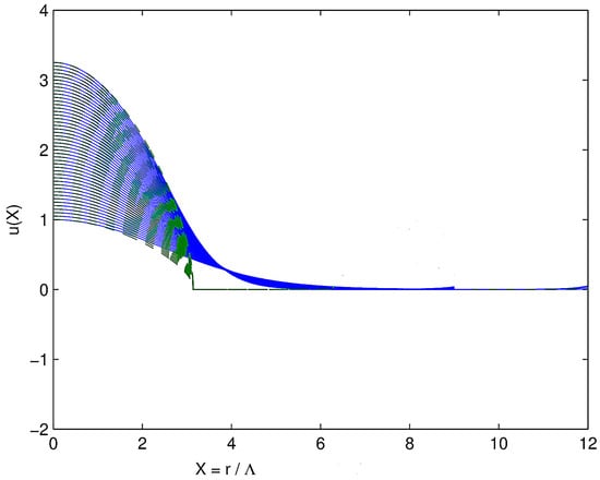
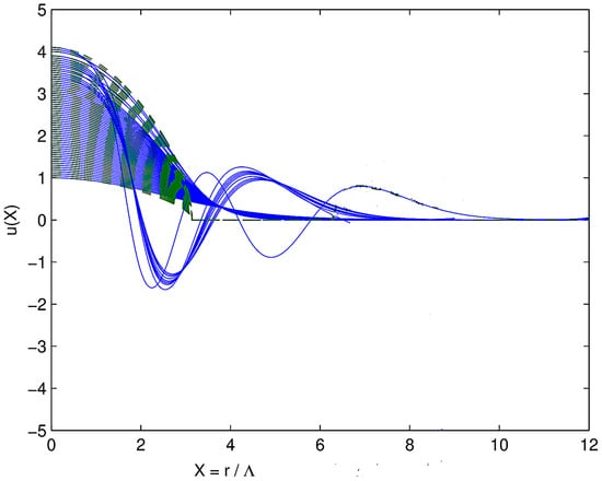
Numerical solutions of the GPP system were obtained by progressively increasing the central amplitude of the wave function, which is equivalent to increasing the central density of the configuration. Figure 1 shows the behavior of the solutions as the central value of the wave function (or, equivalently, the relative central density) is varied in the range $1.00<u_0<3.27$, corresponding to a reduced particle number in the interval $6.19<\kappa <38.05$. In this regime, only ground-state (nodeless) solutions are found, and they agree well with the Thomas–Fermi approximation, as illustrated in Figure 1.

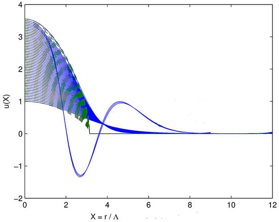
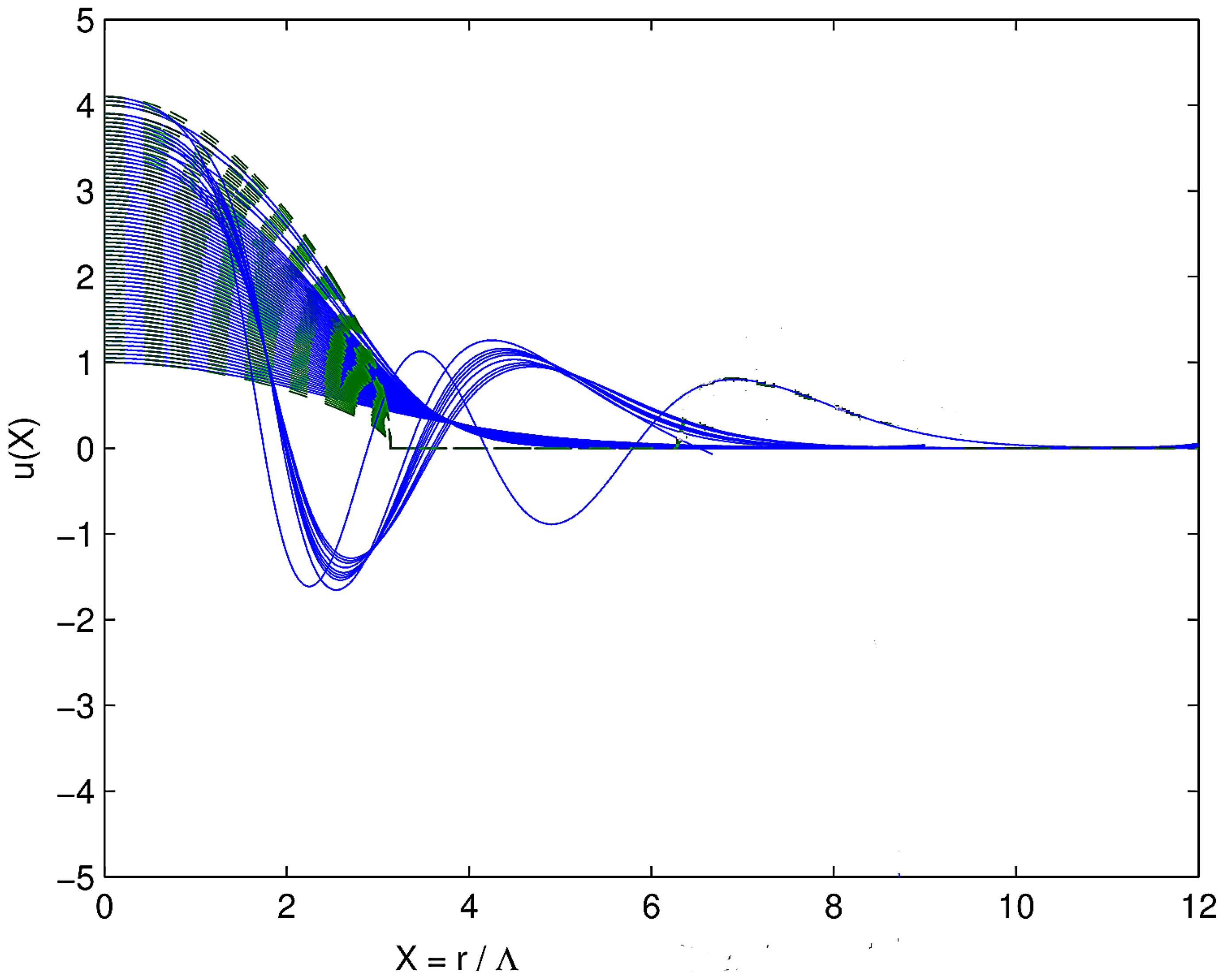
As the central amplitude $u_0$ is increased further, the first excited state, characterized by a two-node wave function, appears once the critical value $u_0\simeq 3.3$ is exceeded, as shown in Figure 2. However, for amplitudes larger than $u_0\sim 3.5$, the ground state reappears. A further increase in $u_0$ leads to the emergence of a four-node excited state with a reduced particle number $\kappa \simeq 80$. This is shown in Figure 3.

Although the present computations correspond to a sequence of stationary configurations, they suggest that when the system occupies an excited state, small variations in the number of particles may trigger transitions toward ground-state configurations with fewer particles. To determine whether the apparent discreteness observed in the $(u_0-\kappa )$ plane could be a numerical artifact, we inverted the calculations by decreasing the central amplitude using slightly different step sizes. The same qualitative behavior was recovered, indicating that this feature is intrinsic to the nonlinear nature of the system. This strongly suggests the presence of bifurcation points that modify the topological structure of the solution space. In other words, nonlinear systems may have bifurcation points corresponding to parameter values at which the number or type of equilibrium solutions changes, or new solution branches appear (or disappear) as our numerical solutions indicate.

This behavior is qualitatively similar to that reported in Ref. [11], where solutions of the Newtonian limit of the Einstein–Klein–Gordon equations were studied. In the plane defined by the total mass and the number of particles, configurations corresponding to a fixed excitation level exhibit a mass that increases with particle number until a critical point (a cusp) is reached. Beyond this point, a new branch emerges in which configurations possess higher masses but fewer particles, until a second cusp is encountered. In this new branch, which is always shorter than the preceding one, the mass again increases with particle number, and the process repeats at successive bifurcation points.

Dynamical studies of boson star collapse without self-interactions reported in Ref. [29] showed that collapsing configurations can eject particles through a process known as gravitational cooling (see also Ref. [30]). These simulations indicate that an initial configuration with a mass exceeding the critical limit by approximately 1.7% loses about 13% of its mass during the collapse. More recently, Ref. [13] investigated the dynamical evolution of boson stars composed of a mixture of two states. Stable configurations were found when the number of particles in the ground state exceeds that in the excited state. In the opposite case, the system becomes unstable and evolves toward a stable configuration through particle emission.

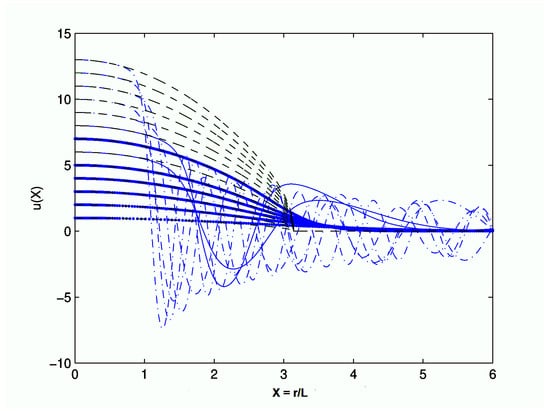
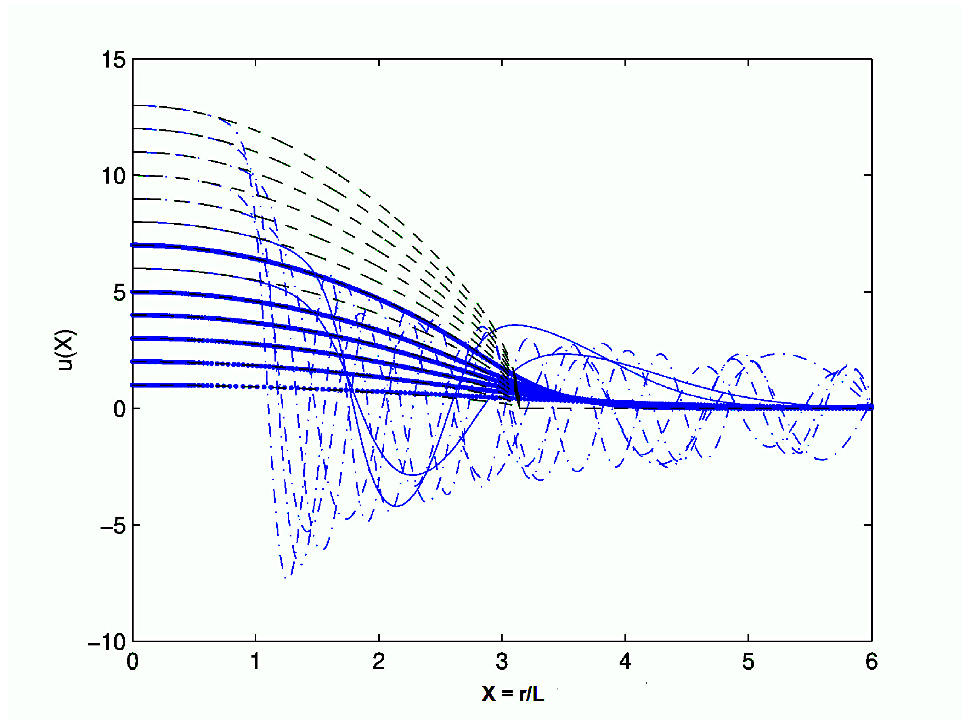
Finally, as the central amplitude is increased beyond $u_0\sim 5.0$, a two-node excited state reappears around $u_0\sim 6.0$, while the ground state is recovered near $u_0\sim 7.0$. At $u_0\sim 8.0$, the two-node state appears once more, and a further increase in $u_0$ leads to increasingly irregular behavior, as illustrated in Figure 4. As we shall see below, solutions defined by central amplitudes $u_0\ge 8.0$ do not satisfy the virial relation and are not expected to be in equilibrium.

For steady configurations ($u_0\le 8.0$), the ground state binding energy (chemical potential) varies approximately linearly with the number of particles, while the width of the eigenstate wave function decreases as $\sqrt{\Lambda }$. The calculated eigenvalues can be fitted approximated by the expression

$$\tilde{\mu }=-0.288\kappa =-{\mu }_0\kappa .$$

(14)

This relation will be used later when the maximum mass of a stable configuration will be estimated.

3.1. The Virial Relation

The stability of the configurations can be studied by estimating the virial relation for models characterized by different parameters. This relation is especially significant in the study of self-gravitating systems, such as bosonic stars or condensates, which can form due to the gravitational collapse. In quantum mechanics, the virial relation provides a powerful relationship between the average value of kinetic and potential energy of a quantum system, particularly in bound systems. Formally, it states that for a stable equilibrium, the average kinetic energy and the effective interaction potential energy are related by the equation, which in our variables is given by

$$\tilde{\mu }+3〈W〉-〈u^2〉=0.$$

(15)

A detailed derivation of this equation is given in Appendix A.

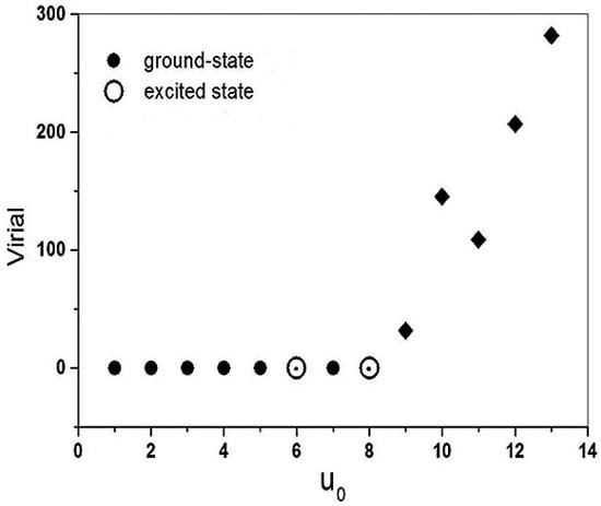
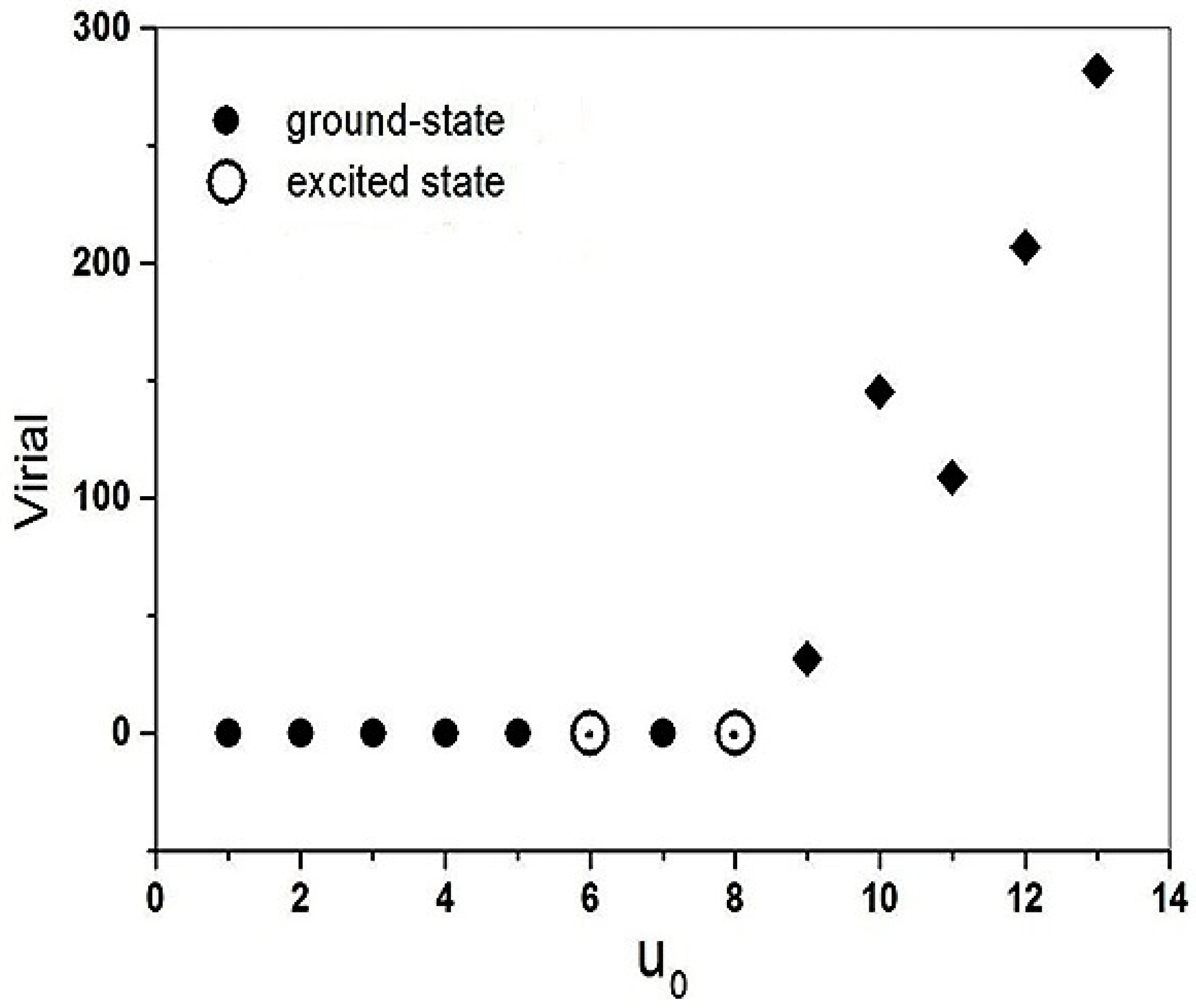
For central amplitudes $u_0\le 8$, our numerical computations indicate that the virial relation is satisfied by equilibrium configurations corresponding to both ground and excited states, as illustrated in Figure 5. Above the critical density, corresponding to $u_0\simeq 8$ or to a maximum reduced particle number ${\kappa }_{max}\simeq 202$, the virial relation is no longer satisfied. In this regime, the virial becomes positive, indicating that the system departs from equilibrium and is therefore expected to be unstable. This behavior suggests that, beyond the critical point, the balance between gravitational attraction and repulsive self-interactions is no longer sufficient to support stationary configurations.

While some excited-state configurations still satisfy the virial relation, one might be tempted to interpret them as dynamically stable. However, a system can satisfy the virial relation (no global contraction or expansion is present) and still be metastable or even unstable to radial perturbations, since the viral is a necessary condition for dynamical equilibrium, but it is not sufficient for stability. In other words, a system can satisfy the virial theorem and still be metastable because the virial theorem is only a first-order equilibrium condition, not a second-order stability condition. The corresponding particle numbers of these excited configurations exceed those of the ground-state solutions predicted by the Thomas–Fermi approximation. This indicates that such configurations do not represent the true equilibrium state of the system, in the sense discussed in Ref. [10], and should instead be regarded as metastable. Moreover, as mentioned previously, in nonlinear systems the ground state can be in reality a mixed state and unstable against fission. It is therefore expected that these excited configurations decay toward a pure ground state through the emission of particles, known as the gravitational cooling mechanism.

The central critical density depends on the wave function central amplitude and on the coupling constant $\lambda$, e.g.,

$${\rho }_0={\displaystyle \frac{8\pi G{m}^6{c}^2}{{\lambda }^2{\hslash }^4}}\mid u_0{\mid }^2.$$

(16)

In order to evaluate the equation above, an estimate for the coupling constant $\lambda$ is required. This can be obtained from the present results combining the relation between the chemical potential and the reduced number of particles $\kappa$, namely Equation (14) with Equation (5) that is,

$$\lambda =8\pi {\mu }_0{\left({\displaystyle \frac{m}{M_P}}\right)}^2{\kappa }_{max},$$

(17)

where ${\kappa }_{max}\simeq 202$ is the value derived from the present computations at the virial break-up, e.g., $u_0=8.0$. Performing the numerical evaluation of the equation above one obtains $\lambda \simeq 3.1\times {10}^{12}$ m², where the boson mass is in grams. This value agrees quite well with the result derived in Ref. [18] based on a different approach. Replacing the value of $\lambda$ in Equation (16) and using the maximum allowed value of the central amplitude, e.g., $u_0=8.0$ it results ${\rho }_0\simeq 2.6\times {10}^{34}{m}_{eV}^2$ g/cm³ where now the boson mass is in eV. For axion-like bosons, particles with masses around ${10}^{-5}$ eV, the estimated central density is about 10 orders of magnitude higher than that prevailing in the core of neutron stars. This is a consequence that bosons are not subject to the Pauli exclusion principle, unlike neutrons. Hence, no degeneracy pressure limit prevents bosons from reaching extremely high central densities.

3.2. The Critical Mass

A fundamental property of self-gravitating bosonic configurations is the existence of a critical (maximum) mass above which equilibrium solutions cease to exist or become dynamically unstable. This feature is common to both relativistic and nonrelativistic descriptions of boson stars and reflects the competition between gravity, quantum pressure, and possible self-interactions of the scalar field. In the relativistic framework, solutions of the Einstein–Klein–Gordon equations show that boson stars possess a maximum mass along the branch of stable equilibrium configurations, commonly identified with the Kaup limit in the absence of self-interactions, or with its generalizations when repulsive self-interactions are included. Beyond this maximum mass, no stable stationary solutions are found.

In the nonrelativistic regime described by the GPP system, a similar notion of critical mass emerges. Although the GPP equations do not incorporate relativistic effects explicitly, they nevertheless exhibit a limiting mass associated with the breakdown of equilibrium configurations. As the number of particles (or, equivalently, the central density) is increased, solutions approach a critical point beyond which the virial balance can no longer be satisfied. This critical mass, therefore, represents the maximum mass for which a self-gravitating bosonic configuration can remain in equilibrium within the validity of the nonrelativistic approximation.

Within the framework of the present study, the concept of critical mass emerges naturally from the numerical solutions of the GPP system. As shown in the previous sections, equilibrium configurations are parametrized by the central amplitude of the wave function, or equivalently by the reduced particle number $\kappa$. As $\kappa$ is increased, the system follows a sequence of stationary solutions until a critical point is reached beyond which no equilibrium configuration satisfying the virial relation can be found. This behavior provides a clear operational definition of the critical mass within the nonrelativistic GPP approach.

In the nonrelativistic regime, the gravitational mass of the configuration is given by the total rest mass of the particles corrected by the binding energy arising from the GPP equations. Accordingly, the gravitational mass of a boson star in the ground state can be written as

$$M=mN+\mu \left(N\right){\displaystyle \frac{N}{c^2}}.$$

(18)

For ground-state configurations, the present calculations show that the binding energy per particle, characterized by the chemical potential $\mu$, varies linearly with the reduced number of particles $\kappa$, according to Equation (14)

$$\mu =-{\mu }_0{\displaystyle \frac{G{m}^2}{2a_s}}\kappa ,$$

(19)

where the physical constants were restored.

Defining the characteristic mass scale $M_{*}={\lambda }^{1/2}{M}_P^3/m^2$, and making use of the previously introduced dimensionless variables, Equation (18) can be recast in the form

$${\displaystyle \frac{M}{M_{*}}}={\displaystyle \frac{\sqrt{2\pi }}{\lambda }}{\left({\displaystyle \frac{m}{M_P}}\right)}^2\kappa -{\displaystyle \frac{\sqrt{32{\pi }^3}}{{\lambda }^2}}{\mu }_0{\left({\displaystyle \frac{m}{M_P}}\right)}^4{\kappa }^2.$$

(20)

In this expression, the scattering length has been replaced by the coupling constant $\lambda$ according to Equation (5). The maximum value of $\kappa$ is obtained from the condition $d(M/M_{*})/d\kappa =0$, which yields

$${\kappa }_{max}={\displaystyle \frac{\lambda }{8\pi {\mu }_0}}{\left({\displaystyle \frac{M_p}{m}}\right)}^2.$$

(21)

This result was already used in the previous section to estimate the coupling constant $\lambda$, since the present numerical analysis gives ${\kappa }_{max}\simeq 202$. Substituting Equation (21) into Equation (20), one obtains for maximum mass

$$M_{max}={\displaystyle \frac{1}{4\sqrt{8\pi }{\mu }_0}}{\lambda }^{1/2}{\displaystyle \frac{M_P^3}{m^2}}=0.173{\lambda }^{1/2}{\displaystyle \frac{M_P^3}{m^2}}.$$

(22)

The numerical coefficient appearing in this expression is approximately 2.8 times larger than that obtained in Ref. [10] from a fully relativistic analysis. Such a difference is not only due to relativistic effects but also to the fact that at high energies, the hard-sphere potential overestimates the pressure resulting from the $\lambda {\varphi }^4$ theory, and therefore for a given central density, more massive configurations result. For axion-like bosons with masses of order ${10}^{-5}$ eV, the resulting maximum mass is of the order of 30 Earth masses, a quite small value despite the fact that the corresponding central densities exceed nuclear densities by several orders of magnitude.

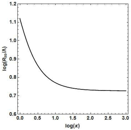
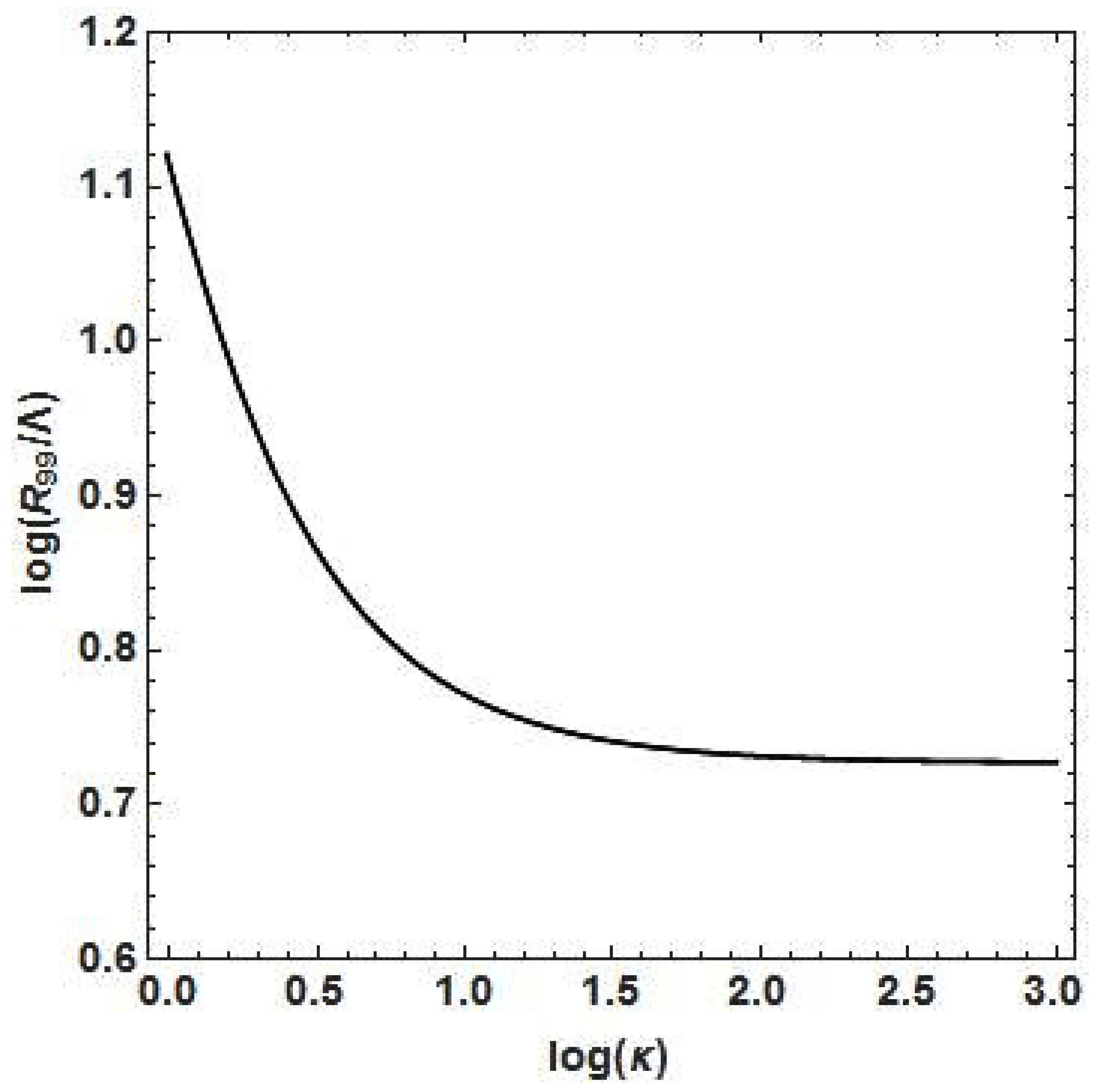
Ground-state solutions are nodeless and formally extend to infinity, which makes the definition of a sharp stellar radius ambiguous. In practice, the size of the boson star is characterized by the radius $R_{99}$, defined as the radius enclosing 99% of the total particle number. Figure 6 shows the dependence of the dimensionless radius $R_{99}/\Lambda$ on the reduced number of particles $\kappa$. For $\kappa <10$, the effective radius scales approximately as $R_{99}\propto {\kappa }^{-1}$, whereas for large particle numbers, the radius approaches a nearly constant value, $R_{99}\simeq 5.33\Lambda$, values consistent with the results derived in Refs. [21,22]. Notice that the characteristic length scale $\Lambda$ can be expressed uniquely in terms of the Compton wavelength of the boson,

$$\Lambda =\sqrt{{\mu }_0{\kappa }_{max}}{\displaystyle \frac{\hslash }{mc}}.$$

(23)

Using this relation and inserting numerical values, one finds that for large particle numbers the typical size of boson stars is $R_{99}\simeq 80$ cm for a boson mass of ${10}^{-5}$ eV. This extreme compactness naturally explains the very high central densities obtained in the present models. However, since ${\rho }_0\propto m^2$, $M_{max}\propto m^{-1}$ and $\Lambda \propto m^{-1}$, lighter bosons will lead to more massive configurations having smaller central densities and larger sizes.

4. Conclusions

In the present work, we have reported new numerical solutions of the nonlinear Gross–Pitaevskii–Poisson system of equations with the aim of investigating the equilibrium and stability properties of boson stars in the nonrelativistic regime. By adopting an appropriate coordinate transformation together with a specific rescaling of the gravitational potential, the resulting system of equations becomes independent of the physical parameters characterizing the model. Within this formulation, equilibrium solutions are fully specified by the usual boundary conditions and by the central value of the dimensionless wave function, which uniquely determines the central density of the configuration once physical units are restored.

Numerical solutions were obtained by incrementing the central amplitude of the wave function using a fine grid. Although only stationary configurations were computed, the analysis revealed the presence of bifurcation points at which transitions between ground-state and excited-state solutions occur. The results further suggest the existence of a limiting value of the central amplitude beyond which the solutions become increasingly irregular, possibly involving mixtures of different states, signaling the breakdown of simple equilibrium configurations as shown in Figure 4.

The virial relation was evaluated for a wide class of models corresponding to both ground and excited states. Previous investigations have shown that virialized ground-state configurations are dynamically stable against small perturbations [30]. In the present study, we find that the virial relation is satisfied only for configurations whose central amplitude lies below a critical value. This implies that stable equilibrium configurations cannot possess central densities exceeding a well-defined critical limit, in agreement with earlier analyses based on the evolution of radial oscillations [18]. Remarkably, this critical density exceeds typical nuclear densities by several orders of magnitude if axion-like bosons with masses of order ${10}^{-5}$ eV are considered.

As shown in Figure 5, some excited-state configurations also satisfy the virial relation, which might suggest dynamical stability. However, since these configurations contain a number of particles larger than the corresponding ground-state solutions predicted by the Thomas–Fermi approximation, they should be regarded as metastable. Such states are therefore expected to decay toward the ground state through particle emission, most likely via the gravitational cooling mechanism (see, for instance, Ref. [30]).

For central densities exceeding the critical value, the virial becomes positive, indicating a loss of equilibrium and the onset of instability. In this regime, the gravitational attraction is no longer sufficient to counterbalance the repulsive self-interactions. The ultimate fate of such unstable configurations remains an open question and depends on relativistic effects not captured by the GPP system. Fully relativistic numerical simulations have shown that unstable boson stars with negative binding energy tend to collapse and form black holes, whereas configurations with positive binding energy disperse to infinity [31,32]. Other studies have identified multiple possible end states, including collapse, dispersal, or relaxation toward a less compact stable configuration, highlighting the rich dynamical behavior of unstable bosonic systems [33,34].

An estimate of the boson-star size was obtained by defining the radius $R_{99}$ enclosing 99% of the total number of particles. For the same boson mass, namely ${10}^{-5}$ eV, we find $R_{99}\simeq 80$ cm, indicating an extremely compact object, which naturally explains the very high central densities found in the present models. Finally, the ratio between the Schwarzschild radius and the effective stellar radius is found to be $R_{Sch}/R_{99}\simeq 0.32$, indicating that the configurations considered here lie close to the limit of validity of the Newtonian approximation.

References

- Böhmer, C.G.; Harko, T. Can dark matter be a Bose-Einstein condensate? J. Cosm. Astr. Phys. 2007, 2007, 025B. [Google Scholar] [CrossRef] [Scilit]
- Feng, J.L. Dark matter candidates from particle physics and methods of detection. Ann.Rev.Astron.Astrophys. 2010, 48, 495–545. [Google Scholar] [CrossRef] [Scilit]
- Haghani, Z.; Harko, T. Bose-Einstein Condensate dark matter with logarithmic nonlinearity. Phys. Rev. D 2026, 113, 044005. [Google Scholar] [CrossRef] [Scilit]
- Indjin, M.; Liu, I.-K.; Proukakis, N.P.; Rigopoulos, G. Virialized profiles and oscillations of self-interacting fuzzy dark matter solitons. Phys. Rev. D 2024, 109, 103518. [Google Scholar] [CrossRef] [Scilit]
- Stallovits, M.; Rindler-Daller, T. Single and merger solition dynamics in scalar field dark matter with and without self-interaction. Phys. Rev. D 2025, 111, 023046. [Google Scholar] [CrossRef] [Scilit]
- Schunck, F.E.; Mielke, E.W. General Relativistic Boson Stars. Class. Quantum Gravity 2003, 20, R301–R356. [Google Scholar] [CrossRef] [Scilit]
- Liebling, S.L.; Palenzuela, C. Dynamical Boson Stars. Living Rev. Rel. 2012, 15, 6. [Google Scholar] [CrossRef] [Scilit]
- Kaup, D.J. Klein-Gordon Geon. Phys. Rev. 1968, 172, 1331–1342. [Google Scholar] [CrossRef] [Scilit]
- Ruffini, R.; Bonazzola, S. Systems of Self-Gravitating Particles in General Relativity and the Concept of an Equation of State. Phys. Rev. 1969, 187, 1767–1783. [Google Scholar] [CrossRef] [Scilit]
- Colpi, M.; Shapiro, S.L.; Wasserman, T. Boson Stars: Gravitational Equilibria of Self-Interacting Scalar Fields. Phys. Rev. Lett. 1986, 57, 2485–2488. [Google Scholar] [CrossRef] [Scilit]
- Friedberg, R.; Lee, T.D.; Pang, Y. Mini-Soliton Stars. Phys. Rev. D 1987, 35, 3640–3657. [Google Scholar] [CrossRef] [Scilit] [PubMed]
- Van der Bij, J.J.; Gleiser, M. Stars of Bosons with Non-Minimal Energy-Momentum Tensor. Phys. Lett. B 1987, 194, 482–486. [Google Scholar] [CrossRef] [Scilit]
- Bernal, A.; Barranco, J.; Alic, D.; Palenzuela, C. Multistate boson stars. Phys. Rev. D 2010, 81, 04403. [Google Scholar] [CrossRef] [Scilit]
- Ureña-López, L.A.; Bernal, A. Bosonic gas as a galactic dark matter halo. Phys. Rev. D 2010, 82, 123535. [Google Scholar] [CrossRef] [Scilit]
- Reinisch, G.; Gudmundsson, V. Nonlinear Interference in a Mean-Field Quantum Model. Eur. Phys. J. B 2011, 84, 699–705. [Google Scholar] [CrossRef] [Scilit]
- Reinisch, G.; Gazeau, M. Role of nonlinearity in non-Hermitian quantum mechanics: Description of linear quantum electrodynamics from the nonlinear Schrödinger-Poisson equation. Eur. Phys. J. Plus 2016, 131, 220. [Google Scholar] [CrossRef] [Scilit]
- Gleiser, M. Stability of Boson Stars. Phys. Rev. D 1988, 38, 2376–2385. [Google Scholar] [CrossRef] [Scilit]
- Jetzer, P. Dynamical Instability of Bosonic Stellar Configurations. Nucl. Phys. B 1989, 316, 411–428. [Google Scholar] [CrossRef] [Scilit]
- Jetzer, P. Stability of Excited Bosonic Stellar Configurations. Phys. Lett. B 1989, 222, 447–452. [Google Scholar] [CrossRef] [Scilit]
- de Freitas Pacheco, J.A.; Peirani, S. Dark matter in the Universe. Int. J. Mod. Phys. D 2004, 13, 1335–1344. [Google Scholar] [CrossRef] [Scilit]
- Chavanis, P.-H. Mass-radius relation of Newtonian self-gravitating Bose-Einstein condensates with short-range interactions: I. Analytical results. Phys. Rev. D 2011, 84, 043531. [Google Scholar] [CrossRef] [Scilit]
- Chavanis, P.-H.; Delfini, L. Mass-radius relation of Newtonian self-gravitating Bose-Einstein condensates with short-range interactions: II. Numerical results. Phys. Rev. D 2011, 84, 043532. [Google Scholar] [CrossRef] [Scilit]
- Schroven, K.; List, M.; Lämerzahl, C. Self-gravitating Bose-Einstein condensates: Excited solutions and stability. In Proceedings of the Fourteenth Marcel Grossmann Meeting, Rome, Italy, 12–18 July 2017; pp. 2043–2048. [Google Scholar] [CrossRef] [Scilit]
- Tena-Contreras, C.; Guzmán, F.S.; Álvarez-Ríos, I. Construction of ground state solutions of the Gross-Pitaevskii-Poisson system using genetic algorithms. Universe 2024, 10, 309. [Google Scholar] [CrossRef] [Scilit]
- Donoghue, J.F.; Sateesh, K.S. Diquark clusters in the quark-gluon plasma. Phys. Rev. D 1988, 38, 360–365. [Google Scholar] [CrossRef] [Scilit] [PubMed]
- Horvath, J.E.; de Freitas Pacheco, J.A.; Araújo, J.C.N. Diquark abundance in stellar matter. Phys. Rev. D 1992, 46, 4754–4757. [Google Scholar] [CrossRef] [Scilit] [PubMed]
- Toth, V.T. Self-gravitating Bose-Einstein condensates and the Thomas-Fermi approximation. Galaxies 2016, 4, 9. [Google Scholar] [CrossRef] [Scilit]
- Kull, H.J. Theory of Rayleigh-Taylor instability. Phys. Rep. 1991, 206, 197–325. [Google Scholar] [CrossRef] [Scilit]
- Seidel, E.; Suen, W.-M. Formation of Solitonic Stars through Gravitational Cooling. Phys. Rev. Lett. 1994, 72, 2516–2519. [Google Scholar] [CrossRef] [Scilit]
- Guzmán, F.S.; Urẽna-López, L.A. Gravitational cooling of self-gravitating Bose-Condensates. Astrophys. J. 2006, 645, 814–819. [Google Scholar] [CrossRef] [Scilit]
- Shibata, M.; Nakamura, T. Evolution of three-dimensional gravitational waves: Harmonic slicing case. Phys. Rev. D 1995, 52, 5428–5444. [Google Scholar] [CrossRef] [Scilit]
- Baumgarte, T.W.; Shapiro, S.L. Numerical integration of Einstein’s field equations. Phys. Rev. D 1999, 59, 024007. [Google Scholar] [CrossRef] [Scilit]
- Guzmán, F.S. The three dynamical fates of boson stars. Rev. Mex. Fis. 2009, 55, 321–326. [Google Scholar]
- Lai, C.W.; Choptuik, M.W. Final fate of subcritical evolutions of boson stars. arXiv 2007, arXiv:0709.0324. [Google Scholar] [CrossRef] [Scilit]
Disclaimer/Publisher’s Note: The statements, opinions and data contained in all publications are solely those of the individual author(s) and contributor(s) and not of MDPI and/or the editor(s). MDPI and/or the editor(s) disclaim responsibility for any injury to people or property resulting from any ideas, methods, instructions or products referred to in the content. |
© 2026 by the authors. Licensee MDPI, Basel, Switzerland. This article is an open access article distributed under the terms and conditions of the Creative Commons Attribution (CC BY) license.