Robust Stability of Quaternion-Valued Neural Networks with Multiple Time Delays and Parameter Uncertainty

Abstract

In this paper, a non-decomposition approach is adopted to study the robust stability of quaternion-valued neural networks (QVNNs) with leakage, discrete, and neutral time delays, and the parameter uncertainty is also considered. The existence and uniqueness of the equilibrium of QVNNs are proved by the homogeneous mapping theorem. By constructing appropriate Lyapunov functions and employing quaternion modulus inequality techniques, sufficient conditions for the global robust stability of QVNNs are presented. Notably, the considered QVNN is treated as a whole rather than being decomposed into complex-valued neural networks (CVNNs) or real-valued neural networks (RVNNs), which faithfully reflects the internal connections between quaternion neurons. Two numerical examples are used to verify the validity of the obtained conclusions.

1. Introduction

In recent decades, RVNNs and CVNNs have garnered extensive attention due to their widespread applications in various fields, such as associative memory, combinatorial optimization, and quantum communication, among others [1,2,3,4,5,6]. However, RVNNs and CVNNs still have certain limitations in practical applications. For example, in signal processing, when dealing with three-dimensional or multidimensional data, multiple real-valued or complex-valued neurons are required. Although this method is feasible, it significantly increases the dimension of the model, thereby increasing the computational complexity. Additionally, this may lead to the loss of some information related to the amplitude and phase of the signal, as the dimensions within multidimensional data are closely interrelated. In contrast, using quaternions directly can make the calculation more efficient and prevent information loss. QVNNs have significant advantages in handling high-dimensional data, such as in color image processing [7], 3D wind prediction [8], and target recognition [9]. Currently, extensive research has been conducted on the dynamical characteristics of QVNNs [10,11,12,13,14].

Due to limitations in the switching speed of amplifiers, time delays inevitably arise in neural systems. The presence of these time delays can introduce more complex dynamical characteristics into neural network systems, sometimes leading to poor performance, such as instability, chaos, and bifurcation [15,16]. Based on their different characteristics, time delays can be classified into several types, including leakage delays [17,18], discrete delays [19,20,21], and neutral delays [22,23,24]. In [25], Xu et al. investigated the Hopf bifurcation problem of fractional QVNNs with leakage delay. In [26], Zhao et al. studied the quasi-synchronization phenomenon of discrete-time fractional quaternion-valued memristive neural networks with time delay and uncertain parameters. These studies only considered a single type of time delay. This limitation has motivated researchers to incorporate multiple time delays into neural networks, which more accurately reflect practical complexities. In this paper, these three types of time delays—leakage, discrete, and neutral delays—are simultaneously considered in the stability analysis of neural networks.

In the practical application of neural networks, the stability of the system is a crucial factor. However, when designing neural networks, due to factors such as modeling errors and environmental disturbances, neural networks often exhibit parameter uncertainty [27,28]. This uncertainty mainly stems from two aspects: firstly, during the parameter estimation stage, key parameters, such as the firing rate of neurons and connection weights, are estimated through statistical methods, which introduces modeling errors; secondly, in the hardware implementation stage, the inherent tolerances of electronic components can cause deviations in network parameters. When neural networks possess such parameter uncertainty characteristics, the stability analysis will face greater challenges. In recent years, various methods for the stability analysis of neural networks with parameter uncertainty have been developed [29,30,31]. Among them, robust control methods (such as $H_{\infty }$ control and sliding mode control) usually suppress the influence of uncertainty by designing feedback controllers, but their design process is complex and difficult to extend to quaternion systems. This paper adopts the method of interval uncertainty model combined with linear matrix inequality (LMI), because it can directly handle the range of parameter perturbations and is convenient for numerical verification. It has been widely applied in RVNNs, CVNNs, and even QVNNs [32,33,34,35,36].

It is well known that quaternions cannot be compared in magnitude and that their multiplication operation does not satisfy the commutative law. Therefore, the research on QVNNs is more challenging compared to RVNNs or CVNNs. To analyze the stability of QVNNs, some scholars have employed decomposition methods, converting them into two CVNNs or four RVNNs [37,38,39] and then establishing corresponding stability criteria. Although this method has certain feasibility, its decomposition process will disrupt the intrinsic geometric structure of the quaternion system and the coupling relationship between neurons, resulting in the loss or weakening of the original rotational invariance and directional information of the system in the subsystems. Moreover, the decomposed subsystems often require additional coordination constraints, which not only increase the complexity and computational burden of the analysis, but may also lead to overly stringent stability conditions. At present, few studies employ non-decomposition methods, rendering the use of such approaches challenging.

Inspired by the above discussion, this paper adopts a direct method to study the robust stability of QVNNs with multiple time delays and parameter uncertainties. From a methodological perspective, this study employs mature analytical tools that are widely used in the stability analysis of delayed neural systems: a Lyapunov–Krasovskii functional is constructed to investigate the effects of leakage, discretization, and neutral-type time delays; LMI techniques are utilized to derive sufficient stability conditions; and the modulus inequality of quaternions is introduced to handle non-commutative multiplication operations. All of these are commonly used tools in the stability analysis of delayed neural networks. The main contributions of this article are as follows:

• This is the first study to integrate leakage, discrete, and neutral delays within a unified QVNN framework while considering parameter uncertainties. The existing studies on QVNN usually only focus on one or two types of delays, while this paper takes into account all three types of delays simultaneously.
• Unlike many previous studies that decompose QVNNs into equivalent real-valued or complex-valued systems, we directly analyze the QVNNs as an integrated quaternion-valued system. This approach preserves the algebraic structure of quaternions and avoids the complications arising from non-commutative multiplication, thereby providing a more natural and concise stability analysis.
• The proposed LMI conditions explicitly account for interval-type parameter uncertainties in all weight matrices, which enhances the practical applicability of the results in real-world implementations where exact parameter values are often unavailable.

The remainder of this paper is summarized below. Some lemmas and assumptions required for the proof are presented, and model descriptions are also provided in Section 2. The sufficient conditions to guarantee the uniqueness, existence and global robust stability of the equilibrium point are derived in Section 3. Two numerical examples are given to verify the validity of the proposed results in Section 4. Conclusions are made in Section 5.

Notations: Let $\mathbb{R},\mathbb{C}\mathrm{and}\mathbb{H}$ denote real, complex and quaternionic skew fields, respectively. Let ${\mathbb{R}}^{n\times m}$, ${\mathbb{C}}^{n\times m}$ and ${\mathbb{H}}^{n\times m}$ denote $n\times m$ matrices from $\mathbb{R}$, $\mathbb{C}$ and $\mathbb{H}$ respectively. Let ${\mathbb{R}}_d^{n\times n}$ denote $n\times n$ real diagonal matrices. $\overline{A}$ denotes the conjugate of A, $A^T$ denotes the transpose of A, and $A^{*}$ denotes the conjugate transpose of A. For $A={\left(a_{ij}\right)}_{n\times n}\in {\mathbb{C}}^{n\times n}$, $∥A∥=\sqrt{{\sum }_{i=1}^n{\sum }_{j=1}^n{\left|a_{ij}\right|}^2}$ denotes the norm of A. $I_n$ is the $n\times n$ identity matrix. ${\lambda }_{max}\left(A\right)$ and ${\lambda }_{min}\left(A\right)$ represent the largest and the smallest eigenvalue of matrix A, respectively. The notation $X\ge Y$ (respectively, $X>Y$) means that $X-Y$ is positive semi-definite (respectively, positive definite). Moreover, the notation $★$ denotes the conjugate transpose of a suitable block in a Hermitian matrix.

2. Preliminaries

Quaternion is a type of hypercomplex numbers that extend from complex numbers. Complex numbers consist of real numbers plus imaginary units i. Similarly, each quaternion is a linear combination of 1, i, j and k, i.e., $q=a+bi+cj+dk$, where a, b, c, and $d\in \mathbb{R}$, as well as the imaginary units i, j, and k, comply with the Hamilton rule, as shown in

Table 1. Hamilton rule.

	1	i	j	k
1	1	i	j	k
i	i	−1	k	−j
j	j	−k	−1	i
k	k	j	−i	−1

. Here, a is represented by $Re\left(q\right)$, and $bi+cj+dk$ is represented by $Im\left(q\right)$.

$q^{*}=\overline{q}=a-bi-cj-dk$ is the conjugate transpose of q. The modulus of the quaternion q is $\left|q\right|=\sqrt{q{q}^{*}}=\sqrt{a_1^2+b_1^2+c_1^2+d_1^2}$. Moreover, $u={(u_1,u_2,\cdots ,u_n)}^T\in {\mathbb{H}}^n$, $\left|u\right|={(\left|u_1\right|,\left|u_2\right|,\cdots ,\left|u_n\right|)}^T$ and $∥u∥=\sqrt{{\sum }_{\mathrm{i}=1}^n{\left|u_i\right|}^2}$.

In this paper, define a partial order ≤ over $\mathbb{H}$: for p, $q\in \mathbb{H}$, $p\le q$ if and only if $a_1\le a_2$, $b_1\le b_2$, $c_1\le c_2$ and $d_1\le d_2$, where $q_1=a_1+b_{1}i+c_{1}j+d_{1}k$ and $q_2=a_2+b_{2}i+c_{2}j+d_{2}k$. Then, define a partial order ≤ over ${\mathbb{H}}^{n\times n}$: for A, $B\in {\mathbb{H}}^{n\times n}$, $A\le B$ if only if $a_{ij}\le b_{ij}$$(i,j=1,2,\cdots ,n)$, where $A={\left(a_{ij}\right)}_{n\times n}$ and $B={\left(b_{ij}\right)}_{n\times n}$.

Lemma 1

([40]). For any $x,y\in {\mathbb{H}}^n$, if $P\in {\mathbb{H}}^{n\times n}$ is a positive definite Hermitian matrix, then

$$x^{*}y+y^{*}x\le x^{*}Px+y^{*}{P}^{-1}{y}^{*}.$$

Lemma 2

([40]). Let $A\in {\mathbb{H}}^{n\times n}$, $\stackrel{\vee }{A}={\left({\stackrel{\vee }{a}}_{ij}\right)}_{n\times n}\in {\mathbb{H}}^{n\times n}, \stackrel{\wedge }{A}={\left({\stackrel{\wedge }{a}}_{ij}\right)}_{n\times n}\in {\mathbb{H}}^{n\times n}$, and $\stackrel{\vee }{A}\le A\le \stackrel{\wedge }{A}$ for any $x,y\in {\mathbb{H}}^{n\times n}$, then the following inequality holds:

$$x^{*}{A}^{*}Ax\le {\left|x\right|}^{*}{\left|A\right|}^{*}\left|A\right|\left|x\right|\le {\left|x\right|}^{*}{\tilde{A}}^{*}\tilde{A}\left|x\right|,$$

$$x^{*}{A}^{*}y+y^{*}Ax\le 2{\left|x\right|}^{*}{\left|A\right|}^{*}\left|y\right|\le 2{\left|x\right|}^{*}{\tilde{A}}^{*}\left|y\right|,$$

where $\tilde{A}={\left({\tilde{a}}_{ij}\right)}_{n\times n}, {\tilde{a}}_{ij}=max\left\{\left|{\stackrel{\vee }{a}}_{ij}\right|,\left|{\stackrel{\wedge }{a}}_{ij}\right|\right\}$.

Lemma 3

([41]). If a continuous map $H\left(z\right):{\mathbb{H}}^n\to {\mathbb{H}}^n$ satisfies the following conditions

(i) 

$H\left(z\right)$ is a injective on ${\mathbb{H}}^n$ and

(ii) 

${\displaystyle \underset{∥z∥\to \infty }{lim}}∥H\left(z\right)∥=\infty$,

then $H\left(z\right)$ is a homeomorphism of ${\mathbb{H}}^n$ onto itself.

Lemma 4

([42]). Let $S=\left(\begin{array}{cc}{S}_{11}& S_{12}\\ S_{21}^T& S_{22}\end{array}\right)\in {\mathbb{R}}^{n\times n}$ with $S_{11}=S_{11}^T, S_{22}=S_{22}^T$, then $S<0$ is equivalent to one of the following two conditions:

(i) 

$S_{11}<0, S_{22}-S_{12}^T{S}_{11}^{-1}{S}_{12}<0$,

(ii) 

$S_{22}<0, S_{11}-S_{12}{S}_{22}^{-1}{S}_{12}^T<0$.

Lemma 5

([40]). For any positive definite constant Hermitian matrix $W\in {\mathbb{H}}^{n\times n}$ and any scalar function $\omega \left(s\right):\left[a,b\right]\to {\mathbb{H}}^n$ with scalars $a<b$ such that the integrations concerned are well defined, we have the following:

$${\left({\int }_a^b\omega \left(s\right)\mathrm{d}s\right)}^{*}W\left({\int }_a^b\omega \left(s\right)\mathrm{d}s\right)\le (b-a){\int }_a^b{\omega }^{*}\left(s\right)W\omega \left(s\right)\mathrm{d}s.$$

Lemma 6

([40]). Let $x,y\in \mathbb{H}$ and $A,B,P\in {\mathbb{H}}^{n\times n}$, where P is a positive define Hermitian matrix. Then,

(i) 

$\left|x+y\right|\le \left|x\right|+\left|y\right|\mathrm{and}\left|xy\right|=\left|x\right|\left|y\right|$;

(ii) 

${\left(AB\right)}^{*}=B^{*}{A}^{*}$;

(iii) 

${\left(AB\right)}^{-1}=B^{-1}{A}^{-1}$ if $A,B$ are invertible;

(iv) 

${\left(A^{*}\right)}^{-1}={\left(A^{-1}\right)}^{*}$ if A is invertible;

(v) 

there exists an invertible matrix $Q\in {\mathbb{H}}^{n\times n}$, such that $P=Q^{*}Q$.

Remark 1.

Inequality techniques play a crucial role in the stability analysis of neural networks based on the direct Lyapunov method. In the existing literature, the stability criteria for RVNNs and CVNNs usually rely on classical inequalities or LMIs as stability criteria. However, due to the unique non-commutative property of the quaternion algebra system and its four-dimensional space coupling characteristics, these inequality tools based on the real or complex domains cannot be directly extended to the stability analysis of QVNNs. To address this key issue, in Lemma 2, this paper innovatively proposes a quaternion modulus inequality analysis method, providing a new mathematical tool for the robust stability study of time-delay QVNNs. The advantages of this method are as follows: firstly, through modulus operations, the non-commutative obstacle of quaternion multiplication is effectively avoided; secondly, the final derived real-valued LMI form criterion is not only computationally feasible, but also strictly ensures the existence and robust stability of the system equilibrium point.

In this paper, we consider the following QVNN model with multiple time delays:

$$\dot{x}\left(t\right)=-Ax(t-\delta )+Bf\left(x\left(t\right)\right)+Cf\left(x(t-\tau )\right)+D\dot{x}(t-h)+J, t\ge 0,$$

(1)

where $x\left(t\right)=({(x_1\left(t\right),x_2\left(t\right),\cdots ,x_n\left(t\right))}^T\in {\mathbb{H}}^n$ is the state vector of the neural networks with n neurons at time t; $A=diag\left\{a_1,a_2,\cdots ,a_n\right\}\in {\mathbb{R}}_d^{n\times n}$ with $a_i>0(i=1,2,\cdots ,n)$ is the self-feedback connection weight matrix; $B={\left(b_{ij}\right)}_{n\times n}\in {\mathbb{H}}^{n\times n}$, $C={\left(c_{ij}\right)}_{n\times n}\in {\mathbb{H}}^{n\times n}$ and $D={\left(d_{ij}\right)}_{n\times n}\in {\mathbb{H}}^{n\times n}$ are the connection weight matrix, the connection weight matrix of discrete delay term, and the connection weight matrix of neutral delay term, respectively; $J\in {\mathbb{H}}^n$ is the external input vector; $\sigma >0$ is the leakage delay; $\tau >0$ is the discrete delay; and $h>0$ is the neutral delay.

The following Hypothesiss are used throughout this paper:

Hypothesis 1.

The parameters $A,B,C,D,J$ in QVNN (1) are assumed to be in the following sets, respectively:

$$\begin{array}{cc}\hfill A_I& =\left[\stackrel{\vee }{A},\stackrel{\wedge }{A}\right]=\left\{A\in {\mathbb{R}}_d^{n\times n}:\stackrel{\vee }{A}\le A\le \stackrel{\wedge }{A}, \stackrel{\vee }{A}, \stackrel{\wedge }{A},\in {\mathbb{R}}_d^{n\times n}and0<\stackrel{\vee }{A}\le \stackrel{\wedge }{A}.\right\},\hfill \\ \hfill B_I& =\left[\stackrel{\vee }{B},\stackrel{\wedge }{B}\right]=\left\{B\in {\mathbb{H}}^{n\times n}:\stackrel{\vee }{B}\le B\le \stackrel{\wedge }{B}, \stackrel{\vee }{B}, \stackrel{\wedge }{B},\in {\mathbb{H}}^{n\times n}and\stackrel{\vee }{B}\le \stackrel{\wedge }{B}.\right\},\hfill \\ \hfill C_I& =\left[\stackrel{\vee }{C},\stackrel{\wedge }{C}\right]=\left\{C\in {\mathbb{H}}^{n\times n}:\stackrel{\vee }{C}\le C\le \stackrel{\wedge }{C}, \stackrel{\vee }{C}, \stackrel{\wedge }{C},\in {\mathbb{H}}^{n\times n}and\stackrel{\vee }{C}\le \stackrel{\wedge }{C}.\right\},\hfill \\ \hfill D_I& =\left[\stackrel{\vee }{D},\stackrel{\wedge }{D}\right]=\left\{D\in {\mathbb{H}}^{n\times n}:\stackrel{\vee }{D}\le D\le \stackrel{\wedge }{D}, \stackrel{\vee }{D}, \stackrel{\wedge }{D},\in {\mathbb{H}}^{n\times n}and\stackrel{\vee }{D}\le \stackrel{\wedge }{D}.\right\},\hfill \\ \hfill J_I& =\left[\stackrel{\vee }{J},\stackrel{\wedge }{J}\right]=\left\{J\in {\mathbb{H}}^n:\stackrel{\vee }{J}\le J\le \stackrel{\wedge }{J}, \stackrel{\vee }{J}, \stackrel{\wedge }{J},\in {\mathbb{H}}^{n}and\stackrel{\vee }{J}\le \stackrel{\wedge }{J}.\right\}.\hfill \end{array}$$

Moreover, let $\stackrel{\vee }{B}={\left({\stackrel{\vee }{b}}_{ij}\right)}_{n\times n}\in {\mathbb{H}}^{n\times n},\stackrel{\wedge }{B}={\left({\stackrel{\wedge }{b}}_{ij}\right)}_{n\times n}\in {\mathbb{H}}^{n\times n},\stackrel{\vee }{C}={\left({\stackrel{\vee }{c}}_{ij}\right)}_{n\times n}\in {\mathbb{H}}^{n\times n},$$\stackrel{\wedge }{C}={\left({\stackrel{\wedge }{c}}_{ij}\right)}_{n\times n}\in {\mathbb{H}}^{n\times n},\stackrel{\vee }{D}={\left({\stackrel{\vee }{d}}_{ij}\right)}_{n\times n}\in {\mathbb{H}}^{n\times n}$ and $\stackrel{\wedge }{D}={\left({\stackrel{\wedge }{d}}_{ij}\right)}_{n\times n}\in {\mathbb{H}}^{n\times n}.$ Then, define $\tilde{B}={\left({\tilde{b}}_{ij}\right)}_{n\times n},\tilde{C}={\left({\tilde{c}}_{ij}\right)}_{n\times n}$ and $\tilde{D}={\left({\tilde{d}}_{ij}\right)}_{n\times n}$, where ${\tilde{b}}_{ij}=max\left\{\left|{\stackrel{\vee }{b}}_{ij}\right|,\left|{\stackrel{\wedge }{b}}_{ij}\right|\right\},{\tilde{c}}_{ij}=max\left\{\left|{\stackrel{\vee }{c}}_{ij}\right|,\left|{\stackrel{\wedge }{c}}_{ij}\right|\right\},{\tilde{d}}_{ij}=max\left\{\left|{\stackrel{\vee }{d}}_{ij}\right|,\left|{\stackrel{\wedge }{d}}_{ij}\right|\right\}.$

Hypothesis 2.

For $i=1,2,\cdots ,n$, the neuron activation function $f_i$ is continuous and satisfies

$$\begin{array}{c}\hfill \left|f_i\left(u_1\right)-f_i\left(u_2\right)\right|\le l_i\left|u_1-u_2\right|,\forall u_1,u_2\in \mathbb{H},\end{array}$$

where $l_i\in \mathbb{R}.$ Moreover, define $L=\mathrm{diag}\{l_1,l_2,\cdots ,l_n\}.$

3. Main Results

In this section, the existence and uniqueness of the equilibrium point, as well as the global robust stability of QVNN (1), are established. First, the existence and uniqueness of the equilibrium point under parameter uncertainties are proved based on the homeomorphism mapping theorem and the modulus inequality of quaternions. Then, a Lyapunov–Krasovskii functional containing three types of time delays is constructed, and the sufficient conditions for global robust stability are derived by means of LMI techniques.

Theorem 1.

Under Hypothesis 1, QVNN (1) has a unique equilibrium if there exist three real positive definite diagonal matrix $U,V_1,V_2$ such that:

$$\mathsf{\Pi }=\left(\begin{array}{ccc}{\mathsf{\Pi }}_{11}& U\tilde{B}& U\tilde{C}\\ ★& -V_1& 0\\ ★& ★& -V_2\end{array}\right)<0,$$

(2)

where ${\mathsf{\Pi }}_{11}=-U\stackrel{\vee }{A}-\stackrel{\vee }{A}U+L{V}_{1}L+L{V}_{2}L$.

Proof. 

Firstly, construct the following continuous map:

$$H\left(x\right)=-Ax+(B+C)f\left(x\right)+J,x\in {\mathbb{H}}^n.$$

(3)

Now, we shall prove that $H\left(x\right)$ is an injective map on ${\mathbb{H}}^n$. Suppose that there exist $x\ne y\in {\mathbb{H}}^n$ such that $H\left(x\right)=H\left(y\right)$, then one has:

$$\begin{array}{c}0=H\left(x\right)-H\left(y\right)=-A(x-y)+(B+C)\left(f\right(x)-f(y\left)\right).\end{array}$$

(4)

Multiply the left-hand side of (4) by ${(x-y)}^{*}U$, then one can get:

$$0=-{(x-y)}^{*}UA(x-y)+{(x-y)}^{*}U(B+C)(f\left(x\right)-f\left(y\right)).$$

(5)

Then, taking the conjugate transpose of (5) yields:

$$0=-{(x-y)}^{*}A{U}^{*}(x-y)+{\left(f\right(x)-f(y\left)\right)}^{*}(B^{*}+C^{*})U^{*}(x-y).$$

(6)

Under Hypothesis 1, adding (5) and (6) and, by Lemmas 1 and 2, one obtains the following equation:

$$\begin{array}{cc}\hfill 0=& -{(x-y)}^{*}(UA+AU)(x-y)+{(x-y)}^{*}UB(f\left(x\right)-f\left(y\right))\hfill \\ \hfill & +{\left(f\right(x)-f(y\left)\right)}^{*}{B}^{*}U(x-y)+{(x-y)}^{*}UC(f\left(x\right)-f\left(y\right))\hfill \\ \hfill & +{\left(f\right(x)-f(y\left)\right)}^{*}{C}^{*}U(x-y)\hfill \\ \hfill \le & -{(x-y)}^{*}(UA+AU)(x-y)+{(x-y)}^{*}UB{V}_1^{-1}{B}^{*}U(x-y)\hfill \\ \hfill & +{(f\left(x\right)-f\left(y\right))}^{*}{V}_1(f\left(x\right)-f\left(y\right))+{(x-y)}^{*}UC{V}_2^{-1}{C}^{*}U(x-y)\hfill \\ \hfill & +{(f\left(x\right)-f\left(y\right))}^{*}{V}_2(f\left(x\right)-f\left(y\right))\hfill \\ \hfill \le & -{(x-y)}^{*}(UA+AU)(x-y)+{(x-y)}^{*}UB{V}_1^{-1}{B}^{*}U(x-y)\hfill \\ \hfill & +{(x-y)}^{*}L{V}_{1}L(x-y)+{(x-y)}^{*}UC{V}_2^{-1}{C}^{*}U(x-y)\hfill \\ \hfill & +{(x-y)}^{*}L{V}_{2}L(x-y)\hfill \\ \hfill \le & {\left|x-y\right|}^{*}\left[-U\stackrel{\vee }{A}-\stackrel{\vee }{A}U+U\tilde{B}{V}_1^{-1}{\tilde{B}}^{*}U+U\tilde{C}{V}_2^{-1}{\tilde{C}}^{*}U+L{V}_{1}L+L{V}_{2}L\right]\left|x-y\right|\hfill \\ \hfill =& {\left|x-y\right|}^{*}\mathsf{\Omega }\left|x-y\right|,\hfill \end{array}$$

(7)

where $\mathsf{\Omega }=-U\stackrel{\vee }{A}-\stackrel{\vee }{A}U+U\tilde{B}{V}_1^{-1}{\tilde{B}}^{*}U+U\tilde{C}{V}_2^{-1}{\tilde{C}}^{*}U+L{V}_{1}L+L{V}_{2}L$, $V_1$ and $V_2$ are real positive diagonal matrices.

Based on Lemma 4 and the LMI (2), one has:

$$\begin{array}{cc}\hfill & {\mathsf{\Pi }}_{11}-\left(\begin{array}{cc}U\tilde{B}& U\tilde{C}\end{array}\right){\left(\begin{array}{cc}-V_1& 0\\ *& -V_2\end{array}\right)}^{-1}\left(\begin{array}{c}{\tilde{B}}^{*}U\\ {\tilde{C}}^{*}U\end{array}\right)\hfill \\ \hfill =& -U\stackrel{\vee }{A}-\stackrel{\vee }{A}U+U\tilde{B}{V}_1^{-1}{\tilde{B}}^{*}U+U\tilde{C}{V}_2^{-1}{\tilde{C}}^{*}U+L{V}_{1}L+L{V}_{2}L\hfill \\ \hfill =& \mathsf{\Omega }<0.\hfill \end{array}$$

(8)

Combining (7) and (8), we obtain that $x-y=0$, i.e., $x=y$. Therefore, $H\left(x\right)$ is a monomorphism on ${\mathbb{H}}^n$.

Next, we prove $∥H\left(x\right)∥\to \infty \mathrm{as}∥x∥\to \infty$.

Let $\tilde{H}\left(x\right)=H\left(x\right)-H\left(0\right)$, then using Lemmas 1 and 2, one can get:

$$\begin{array}{cc}\hfill x^{*}U\tilde{H}\left(x\right)+{\tilde{H}}^{*}\left(x\right)Ux=& -x^{*}(UA+AU)x+x^{*}UB(f\left(x\right)-f\left(0\right))\hfill \\ \hfill & +{(f\left(x\right)-f\left(0\right))}^{*}{B}^{*}Ux+xUC(f\left(x\right)-f\left(0\right))\hfill \\ \hfill & +{(f\left(x\right)-f\left(0\right))}^{*}{C}^{*}Ux\hfill \\ \hfill \le & -x^{*}(UA+AU)x+x^{*}UB{V}_1^{-1}{B}^{*}Ux+x^{*}UC{V}_2^{-1}{C}^{*}Ux\hfill \\ \hfill & +x^{*}L{V}_{1}Lx+x^{*}L{V}_{2}Lx\hfill \\ \hfill \le & {\left|x\right|}^{*}\left[-U\stackrel{\vee }{A}-\stackrel{\vee }{A}U+U\tilde{B}{V}_1^{-1}{\tilde{B}}^{*}U\right.\hfill \\ \hfill & \left.+U\tilde{C}{V}_2^{-1}{\tilde{C}}^{*}U+L{V}_{1}L+L{V}_{2}L\right]\left|x\right|\hfill \\ \hfill =& {\left|x\right|}^{*}\mathsf{\Omega }\left|x\right|\le -{\lambda }_{min}(-\mathsf{\Omega }){∥x∥}^2.\hfill \end{array}$$

In light of Lemma 2, one has:

$$\begin{array}{cc}\hfill & {\lambda }_{min}(-\mathsf{\Omega }){∥x∥}^2\le -x^{*}U\tilde{H}\left(x\right)-{\tilde{H}}^{*}\left(x\right)Ux=-2Re{x}^{*}U\tilde{H}\left(x\right)\hfill \\ \hfill & \le 2∥x∥∥U∥\left(∥H\left(x\right)-H\left(0\right)∥\right)\le 2∥x∥∥U∥(∥H\left(x\right)∥+∥H\left(0\right)∥),\hfill \end{array}$$

(9)

i.e., ${\lambda }_{min}(-\mathsf{\Omega })∥x∥\le 2∥U∥(∥H\left(x\right)∥+∥H\left(0\right)∥)$, which implies that $∥H\left(x\right)∥\to \infty \mathrm{as}∥x∥\to \infty .$ From Lemma 3, we have that $H\left(x\right)$ is a homomorphic map on ${\mathbb{H}}^n$. Therefore, QVNN (1) has a unique equilibrium point. □

Next, we will prove that the equilibrium point is globally robustly stable.

Theorem 2.

Under Hypothesis 1 and Hypothesis 2, QVNN (1) is globally robustly stable if there exist eleven real positive diagonal matrices $Q_{1,}{Q}_{2,}{Q}_3,Q_4,Q_5,Q_6,Q_{7,}{P}_1,P_2,R_1$ and $R_2$, such that

$$\begin{array}{c}\hfill \tilde{\mathsf{\Pi }}=\left(\begin{array}{ccccccccc}{\tilde{\mathsf{\Pi }}}_{11}& 0& 0& Q_6& Q_1\tilde{D}& Q_1\tilde{B}& Q_1\tilde{C}& 0& \stackrel{\wedge }{A}{Q}_1\stackrel{\wedge }{A}\\ ★& {\tilde{\mathsf{\Pi }}}_{22}& 0& \stackrel{\wedge }{A}{P}_1+P_2& P_2^{*}\tilde{D}& P_2^{*}\tilde{B}& P_2^{*}\tilde{C}& 0& 0\\ ★& ★& {\tilde{\mathsf{\Pi }}}_{33}& 0& 0& 0& 0& 0& 0\\ ★& ★& ★& {\tilde{\mathsf{\Pi }}}_{44}& P_1^{*}\tilde{D}& P_1^{*}\tilde{B}& P_1^{*}\tilde{C}& 0& 0\\ ★& ★& ★& ★& -Q_7& 0& 0& 0& \tilde{D}{Q}_1\stackrel{\wedge }{A}\\ ★& ★& ★& ★& ★& {\tilde{\mathsf{\Pi }}}_{66}& 0& 0& \tilde{B}{Q}_1\stackrel{\wedge }{A}\\ ★& ★& ★& ★& ★& ★& -R_2& 0& \tilde{C}{Q}_1\stackrel{\wedge }{A}\\ ★& ★& ★& ★& ★& ★& ★& -Q_5& 0\\ ★& ★& ★& ★& ★& ★& ★& ★& -Q_3\end{array}\right)<0,\end{array}$$

(10)

where

$$\begin{array}{cc}\hfill & {\tilde{\mathsf{\Pi }}}_{11}=-Q_1\stackrel{\vee }{A}-Q_1\stackrel{\vee }{A}+Q_2+{\delta }^2{Q}_3+Q_4+Q_6+L{R}_{1}L,\hfill \\ \hfill & {\tilde{\mathsf{\Pi }}}_{22}=-Q_2-P_2^{*}\stackrel{\vee }{A}-\stackrel{\vee }{A}{P}_2,{\tilde{\mathsf{\Pi }}}_{33}=-Q_4+L{R}_{2}L,\hfill \\ \hfill & {\tilde{\mathsf{\Pi }}}_{44}=-P_1^{*}-P_1+Q_7,{\tilde{\mathsf{\Pi }}}_{66}=Q_5-R_1.\hfill \end{array}$$

Proof. 

We take the submatrix ${\tilde{\mathsf{\Pi }}}_1$, consisting of rows 1, 6, 7 and columns 1, 6, 7 of $\tilde{\mathsf{\Pi }}$ i.e., ${\tilde{\mathsf{\Pi }}}_1=\left(\begin{array}{ccc}{\tilde{\mathsf{\Pi }}}_{11}& Q_1\tilde{B}& Q_1\tilde{C}\\ ★& Q_5-R_1& 0\\ ★& ★& -R_2\end{array}\right)$; thus, ${\tilde{\mathsf{\Pi }}}_1<0$. Since $Q_2+{\delta }^2{Q}_3+Q_6>0$, and ${\tilde{\mathsf{\Pi }}}_{33}<0$, we can obtain

$$\begin{array}{cc}\hfill {\tilde{\mathsf{\Pi }}}_2& ={\tilde{\mathsf{\Pi }}}_1+\left(\begin{array}{ccc}-Q_2-{\delta }^2{Q}_3-Q_6+{\tilde{\mathsf{\Pi }}}_{33}& 0& 0\\ 0& 0& 0\\ 0& 0& 0\end{array}\right)\hfill \\ \hfill & =\left(\begin{array}{ccc}-Q_1\stackrel{\vee }{A}-Q_1\stackrel{\vee }{A+L{R}_{1}L+L{R}_{2}L}& Q_1\tilde{B}& Q_1\tilde{C}\\ ★& Q_5-R_1& 0\\ ★& ★& -R_2\end{array}\right)<0.\hfill \end{array}$$

(11)

On the other hand, if $U=Q_1>0$, $V_1=-Q_5+R_1>0$, and $V_2=R_2>0$, we will have

$$\begin{array}{c}\hfill \mathsf{\Pi }={\tilde{\mathsf{\Pi }}}_2,\end{array}$$

(12)

where $\mathsf{\Pi }$ is defined in LMI (2) of Theorem 1. From (10) and (11), it follows that LMI (2) holds. Thus, there is only one unique equilibrium for QVNN (1) under Theorem 1.

Let $\stackrel{\vee }{x}$ be the unique equilibrium point of QVNN (1). The equilibrium point $\stackrel{\vee }{x}$ satisfies: $-A\stackrel{\vee }{x}+(B+C)f\left(\stackrel{\vee }{x}\right)+J=0.$

Since the parameters $A, B, C, J$ take values within given bounded intervals, the location of the equilibrium point $\stackrel{\vee }{x}$ is not fixed but varies with the parameters. Specifically, each admissible realization of the parameters corresponds to a unique equilibrium point. Under the parameter uncertainty Hypothesis 1, the equilibrium points $\stackrel{\vee }{x}$ form a set: $\mathcal{E}=\left\{\stackrel{\vee }{x}\in {\mathbb{H}}^n|0=-A\stackrel{\vee }{x}+(B+C)f\left(\stackrel{\vee }{x}\right)+J,A\in A_I,B\in B_I,C\in C_I,J\in J_I\right\}$. Each element in this set represents the equilibrium point of (1) under a certain set of parameters. Next, it will be proved that, for every set of values within the parameter range, the unique equilibrium point of (1) is globally robustly stable.

The equilibrium point $\stackrel{\vee }{x}$ is translated to the origin by $\tilde{x}\left(t\right)=x\left(t\right)-\stackrel{\vee }{x}$. QVNN (1) is transformed into the following:

$$\begin{array}{c}\hfill \dot{\tilde{x}}\left(t\right)=-A\tilde{x}(t-\delta )+Bf\left(\tilde{x}\left(t\right)\right)+Cf\left(\tilde{x}(t-\tau )\right)+D\dot{\tilde{x}}(t-h),\end{array}$$

(13)

where $f\left(\tilde{x}\left(t\right)\right)=f\left(x\left(t\right)\right)-f\left(\stackrel{\vee }{x}\right)$ and $f\left(\tilde{x}(t-\tau )\right)=f\left(x(t-\tau )\right)-f\left(\stackrel{\vee }{x}\right)$.

Consider the following the Lyapunov–Krasovskii function:

$$\begin{array}{c}\hfill V\left(t\right)=\sum _{i=1}^6{V}_i\left(t\right),\end{array}$$

where

$$\begin{array}{cc}\hfill & V_1\left(t\right)={\left(\tilde{x}\left(t\right)-A{\int }_{t-\delta }^t\tilde{x}\left(s\right)\mathrm{d}s\right)}^{*}{Q}_1\left(\tilde{x}\left(t\right)-A{\int }_{t-\delta }^t\tilde{x}\left(s\right)\mathrm{d}s\right),\hfill \\ \hfill & V_2\left(t\right)={\int }_{t-\delta }^t{\tilde{x}}^{*}\left(s\right)Q_2\tilde{x}\left(s\right)\mathrm{d}s,\hfill \\ \hfill & V_3\left(t\right)=\delta {\int }_0^{\delta }{\int }_{t-u}^t{\tilde{x}}^{*}\left(s\right)Q_3\tilde{x}\left(s\right)\mathrm{d}s\mathrm{d}u,\hfill \\ \hfill & V_4\left(t\right)={\int }_{t-\tau }^t{\tilde{x}}^{*}\left(s\right)Q_4\tilde{x}\left(s\right)\mathrm{d}s,\hfill \\ \hfill & V_5\left(t\right)={\int }_{t-h}^t{f}^{*}\left(\tilde{x}\left(s\right)\right)Q_{5}f\left(\tilde{x}\left(s\right)\right)\mathrm{d}s,\hfill \\ \hfill & V_6\left(t\right)={\tilde{x}}^{*}\left(t\right)Q_6\tilde{x}\left(t\right)+{\int }_{t-h}^t{\dot{\tilde{x}}}^{*}\left(s\right)Q_7\dot{\tilde{x}}\left(s\right)\mathrm{d}s.\hfill \end{array}$$

Calculating the derivative of $V_i\left(t\right)(i=1,2,\cdots 6)$, we obtain

$$\begin{array}{cc}\hfill {\dot{V}}_1\left(t\right)=& {\left(\tilde{x}\left(t\right)-A{\int }_{t-\delta }^t\tilde{x}\left(s\right)\mathrm{d}s\right)}^{*}{Q}_1\left(-A\tilde{x}\left(t\right)+Bf\left(\tilde{x}\left(t\right)\right)+Cf\left(\tilde{x}(t-\tau )\right)+D\dot{\tilde{x}}(t-h)\right)\hfill \\ \hfill & +{\left(-A\tilde{x}\left(t\right)+Bf\left(\tilde{x}\left(t\right)\right)+Cf\left(\tilde{x}(t-\tau )\right)+D\dot{\tilde{x}}(t-h)\right)}^{*}{Q}_1\left(\tilde{x}\left(t\right)-A{\int }_{t-\delta }^t\tilde{x}\left(s\right)\mathrm{d}s\right)\hfill \\ \hfill =& -{\tilde{x}}^{*}\left(t\right)(Q_{1}A+A{Q}_1)\tilde{x}\left(t\right)+{\tilde{x}}^{*}\left(t\right)Q_{1}Bf\left(\tilde{x}\left(t\right)\right)+f^{*}\left(\tilde{x}\left(t\right)\right)B^{*}{Q}_1\tilde{x}\left(t\right)\hfill \\ \hfill & +{\tilde{x}}^{*}\left(t\right)Q_{1}Cf\left(\tilde{x}\left(t\right)\right)+f^{*}\left(\tilde{x}\left(t\right)\right)C^{*}{Q}_1\tilde{x}\left(t\right)+{\tilde{x}}^{*}\left(t\right)Q_{1}D\dot{\tilde{x}}(t-h)\hfill \\ \hfill & +{\dot{\tilde{x}}}^{*}(t-h)D^{*}{Q}_1\tilde{x}\left(t\right)+{\left({\int }_{t-\delta }^t\tilde{x}\left(t\right)\mathrm{d}s\right)}^{*}A{Q}_{1}A\tilde{x}\left(t\right)+{\tilde{x}}^{*}\left(t\right)A{Q}_{1}A\left({\int }_{t-\delta }^t\tilde{x}\left(t\right)\mathrm{d}s\right)\hfill \\ \hfill & -{\left({\int }_{t-\delta }^t\tilde{x}\left(t\right)\mathrm{d}s\right)}^{*}A{Q}_{1}Bf\left(\tilde{x}\left(t\right)\right)-f^{*}\left(\tilde{x}\left(t\right)\right)B^{*}{Q}_{1}A\left({\int }_{t-\delta }^t\tilde{x}\left(t\right)\mathrm{d}s\right)\hfill \\ \hfill & -{\left({\int }_{t-\delta }^t\tilde{x}\left(t\right)\mathrm{d}s\right)}^{*}A{Q}_{1}Cf\left(\tilde{x}(t-\tau )\right)-f^{*}\left(\tilde{x}(t-\tau )\right)C^{*}{Q}_{1}A\left({\int }_{t-\delta }^t\tilde{x}\left(t\right)\mathrm{d}s\right)\hfill \\ \hfill & -{\left({\int }_{t-\delta }^t\tilde{x}\left(t\right)\mathrm{d}s\right)}^{*}A{Q}_{1}D\dot{\tilde{x}}(t-h)-{\dot{\tilde{x}}}^{*}(t-h)D^{*}{Q}_{1}A\left({\int }_{t-\delta }^t\tilde{x}\left(t\right)\mathrm{d}s\right),\hfill \end{array}$$

(14)

$${\dot{V}}_2\left(t\right)={\tilde{x}}^{*}\left(t\right)Q_2\tilde{x}\left(t\right)-{\tilde{x}}^{*}(t-\delta )Q_2\tilde{x}(t-\delta ),$$

(15)

$$\begin{array}{cc}\hfill {\dot{V}}_3\left(t\right)& ={\delta }^2{\tilde{x}}^{*}\left(t\right)Q_3\tilde{x}\left(t\right)-\delta {\int }_0^{\delta }{\tilde{x}}^{*}(t-u)Q_3\tilde{x}(t-u)\mathrm{d}u\hfill \\ & ={\delta }^2{\tilde{x}}^{*}\left(t\right)Q_3\tilde{x}\left(t\right)-\delta {\int }_{t-\delta }^t{\tilde{x}}^{*}\left(s\right)Q_3\tilde{x}\left(s\right)\mathrm{d}s\hfill \\ & \le {\delta }^2{\tilde{x}}^{*}\left(t\right)Q_3\tilde{x}\left(t\right)-{\left({\int }_{t-\delta }^t{\tilde{x}}^{*}\left(s\right)\mathrm{d}s\right)}^{*}{Q}_3\left({\int }_{t-\delta }^t{\tilde{x}}^{*}\left(s\right)\mathrm{d}s\right),\hfill \end{array}$$

(16)

$$\begin{array}{cc}\hfill {\dot{V}}_4\left(t\right)=& {\tilde{x}}^{*}\left(t\right)Q_4\tilde{x}\left(t\right)-{\tilde{x}}^{*}(t-\tau )Q_4\tilde{x}(t-\tau ),\hfill \end{array}$$

(17)

$$\begin{array}{cc}\hfill {\dot{V}}_5\left(t\right)=& f^{*}\left(\tilde{x}\left(t\right)\right)Q_{5}f\left(\tilde{x}\left(t\right)\right)-f^{*}\left(\tilde{x}(t-h)\right)Q_{5}f\left(\tilde{x}(t-h)\right),\hfill \end{array}$$

(18)

$$\begin{array}{cc}\hfill {\dot{V}}_6\left(t\right)=& {\dot{\tilde{x}}}^{*}\left(t\right)Q_6\tilde{x}\left(t\right)+{\tilde{x}}^{*}\left(t\right)Q_6\dot{\tilde{x}}\left(t\right)+{\dot{\tilde{x}}}^{*}\left(t\right)Q_7\dot{\tilde{x}}\left(t\right)-{\dot{\tilde{x}}}^{*}(t-h)Q_7\dot{\tilde{x}}(t-h).\hfill \end{array}$$

(19)

In deriving Inequality (16), we have made use of Lemma 5. Then, under the Hypothesis 2, we get

$$\begin{array}{cc}\hfill & 0\le {\tilde{x}}^{*}\left(t\right)L{R}_{1}L\tilde{x}\left(t\right)-f^{*}\left(\tilde{x}\left(t\right)\right)R_{1}f\left(\tilde{x}\left(t\right)\right),\hfill \end{array}$$

(20)

$$\begin{array}{cc}\hfill & 0\le {\tilde{x}}^{*}(t-\tau )L{R}_{2}L\tilde{x}(t-\tau )-f^{*}\left(\tilde{x}(t-\tau )\right)R_{2}f\left(\tilde{x}(t-\tau )\right).\hfill \end{array}$$

(21)

It is obtained from Model (13) that

$$\begin{array}{cc}\hfill 0=& {\left[P_1\dot{\tilde{x}}\left(t\right)+P_2\tilde{x}(t-\delta )\right]}^{*}\left[-\dot{\tilde{x}}\left(t\right)-A\tilde{x}(t-\delta )+Bf\left(\tilde{x}\left(t\right)\right)+Cf\left(\tilde{x}(t-\tau )\right)+D\dot{\tilde{x}}(t-h)\right]\hfill \\ \hfill & +{\left[-\dot{\tilde{x}}\left(t\right)-A\tilde{x}(t-\delta )+Bf\left(\tilde{x}\left(t\right)\right)+Cf\left(\tilde{x}(t-\tau )\right)+D\dot{\tilde{x}}(t-h)\right]}^{*}\left[P_1\dot{\tilde{x}}\left(t\right)+P_2\tilde{x}(t-\delta )\right].\hfill \end{array}$$

(22)

Based on (14)–(22), one can obtain that

$$\begin{array}{cc}\hfill \dot{V}\left(t\right)& \le {\tilde{x}}^{*}\left(t\right)(-Q_{1}A-A{Q}_1+Q_2+{\delta }^2{Q}_3+Q_4+Q_6+L{R}_{1}L)\tilde{x}\left(t\right)\hfill \\ \hfill & +{\tilde{x}}^{*}\left(t\right)Q_{1}Bf\left(\tilde{x}\left(t\right)\right)+f^{*}\left(\tilde{x}\left(t\right)\right)B^{*}{Q}_1\tilde{x}\left(t\right)+{\tilde{x}}^{*}\left(t\right)Q_{1}Cf\left(\tilde{x}(t-\tau )\right)\hfill \\ \hfill & +f^{*}\left(\tilde{x}(t-\tau )\right)C^{*}{Q}_1\tilde{x}\left(t\right)+{\tilde{x}}^{*}\left(t\right)Q_{1}D\dot{\tilde{x}}(t-h)+{\dot{\tilde{x}}}^{*}(t-h)D{Q}_1\tilde{x}\left(t\right)\hfill \\ \hfill & +{\left({\int }_{t-\delta }^t\tilde{x}\left(t\right)\mathrm{d}s\right)}^{*}A{Q}_{1}A\tilde{x}\left(t\right)+{\tilde{x}}^{*}\left(t\right)A{Q}_{1}A\left({\int }_{t-\delta }^t\tilde{x}\left(t\right)\mathrm{d}s\right)\hfill \\ \hfill & +{\left({\int }_{t-\delta }^t\tilde{x}\left(t\right)\mathrm{d}s\right)}^{*}A{Q}_{1}Bf\left(\tilde{x}\left(t\right)\right)+f^{*}\left(\tilde{x}\left(t\right)\right)B{Q}_{1}A\left({\int }_{t-\delta }^t\tilde{x}\left(t\right)\mathrm{d}s\right)\hfill \\ \hfill & +{\left({\int }_{t-\delta }^t\tilde{x}\left(t\right)\mathrm{d}s\right)}^{*}A{Q}_{1}Cf\left(\tilde{x}(t-\tau )\right)+f^{*}\left(\tilde{x}(t-\tau )\right)C{Q}_{1}A\left({\int }_{t-\delta }^t\tilde{x}\left(t\right)\mathrm{d}s\right)\hfill \\ \hfill & +{\left({\int }_{t-\delta }^t\tilde{x}\left(t\right)\mathrm{d}s\right)}^{*}A{Q}_{1}D\dot{\tilde{x}}(t-h)+{\dot{\tilde{x}}}^{*}(t-h)D{Q}_{1}A\left({\int }_{t-\delta }^t\tilde{x}\left(t\right)\mathrm{d}s\right)\hfill \\ \hfill & +{\dot{\tilde{x}}}^{*}\left(t\right)(-P_1^{*}-P_1+Q_7)\dot{\tilde{x}}\left(t\right)+{\dot{\tilde{x}}}^{*}\left(t\right)(-P_1^{*}A-P_2)\tilde{x}(t-\delta )\hfill \\ \hfill & +{\tilde{x}}^{*}(t-\delta )(-A{P}_1-P_2^{*})\dot{\tilde{x}}\left(t\right)+{\dot{\tilde{x}}}^{*}\left(t\right)P_1^{*}Bf\left(\tilde{x}\left(t\right)\right)+f^{*}\left(\tilde{x}\left(t\right)\right)B^{*}{P}_1\dot{\tilde{x}}\left(t\right)\hfill \\ \hfill & +{\dot{\tilde{x}}}^{*}\left(t\right)P_1^{*}Cf\left(\tilde{x}(t-\tau )\right)+f^{*}\left(\tilde{x}(t-\tau )\right)C^{*}{P}_1\dot{\tilde{x}}\left(t\right)\hfill \\ \hfill & +{\dot{\tilde{x}}}^{*}\left(t\right)P_1^{*}D\dot{\tilde{x}}(t-h)+{\dot{\tilde{x}}}^{*}(t-h)D{P}_1\dot{\tilde{x}}\left(t\right)\hfill \\ \hfill & +{\tilde{x}}^{*}(t-\delta )(-Q_2-P_2^{*}A-A{P}_2)\tilde{x}(t-\delta )\hfill \\ \hfill & +{\tilde{x}}^{*}(t-\delta )P_2^{*}Bf\left(\tilde{x}\left(t\right)\right)+f^{*}\left(\tilde{x}\left(t\right)\right)B^{*}{P}_2\tilde{x}(t-\delta )\hfill \\ \hfill & +{\tilde{x}}^{*}(t-\delta )P_2^{*}Cf\left(\tilde{x}(t-\tau )\right)+f^{*}\left(\tilde{x}(t-\tau )\right)C^{*}{P}_2{\tilde{x}}^{*}(t-\delta )\hfill \\ \hfill & +{\tilde{x}}^{*}(t-\delta )P_2^{*}D\dot{\tilde{x}}(t-h)+{\dot{\tilde{x}}}^{*}(t-h)D{P}_2\tilde{x}(t-\delta )\hfill \\ \hfill & +{\tilde{x}}^{*}(t-\tau )(-Q_4+L{R}_{2}L)\tilde{x}(t-\tau )+f^{*}\left(\tilde{x}\left(t\right)\right)(Q_5-R_1)f\left(\tilde{x}\left(t\right)\right)\hfill \\ \hfill & -f^{*}\left(\tilde{x}(t-h)\right)Q_{5}f\left(\tilde{x}(t-h)\right)-f^{*}\left(\tilde{x}(t-\tau )\right)R_{2}f\left(\tilde{x}(t-\tau )\right)\hfill \\ \hfill & +{\dot{\tilde{x}}}^{*}\left(t\right)Q_6\tilde{x}\left(t\right)+{\tilde{x}}^{*}\left(t\right)Q_6\dot{\tilde{x}}\left(t\right)-{\dot{\tilde{x}}}^{*}(t-h)Q_7\dot{\tilde{x}}(t-h)\hfill \\ \hfill & -{\left({\int }_{t-\delta }^t{\tilde{x}}^{*}\left(s\right)\mathrm{d}s\right)}^{*}{Q}_3\left({\int }_{t-\delta }^t{\tilde{x}}^{*}\left(s\right)\mathrm{d}s\right)\hfill \\ \hfill & \le \left|{\tilde{x}}^{*}\left(t\right)\right|(-Q_1\stackrel{\vee }{A}-\stackrel{\vee }{A}{Q}_1+Q_2+{\delta }^2{Q}_3+Q_4+Q_6+L{R}_{1}L)\left|\tilde{x}\left(t\right)\right|\hfill \\ \hfill & +2\left|{\tilde{x}}^{*}\left(t\right)\right|Q_1\tilde{B}\left|f\left(\tilde{x}\left(t\right)\right)\right|+2\left|{\tilde{x}}^{*}\left(t\right)\right|Q_1\tilde{C}\left|f\left(\tilde{x}(t-\tau )\right)\right|\hfill \\ \hfill & +2\left|{\tilde{x}}^{*}\left(t\right)\right|Q_1\tilde{D}\left|\dot{\tilde{x}}(t-h)\right|+2\left|{\tilde{x}}^{*}\left(t\right)\right|\stackrel{\wedge }{A}{Q}_1\stackrel{\wedge }{A}\left|\left({\int }_{t-\delta }^t\tilde{x}\left(t\right)\mathrm{d}s\right)\right|\hfill \\ \hfill & +2\left|f^{*}\left(\tilde{x}\left(t\right)\right)\right|\tilde{B}{Q}_1\stackrel{\wedge }{A}\left|\left({\int }_{t-\delta }^t\tilde{x}\left(t\right)\mathrm{d}s\right)\right|+2\left|f^{*}\left(\tilde{x}(t-\tau )\right)\right|\tilde{C}{Q}_1\stackrel{\wedge }{A}\hfill \\ \hfill & \times \left|\left({\int }_{t-\delta }^t\tilde{x}\left(t\right)\mathrm{d}s\right)\right|+2\left|{\dot{\tilde{x}}}^{*}(t-h)\right|\tilde{D}{Q}_1\stackrel{\wedge }{A}\left|\left({\int }_{t-\delta }^t\tilde{x}\left(t\right)\mathrm{d}s\right)\right|\hfill \\ \hfill & +\left|{\dot{\tilde{x}}}^{*}\left(t\right)\right|(-P_1^{*}-P_1+Q_7)\left|\dot{\tilde{x}}\left(t\right)\right|+2\left|{\dot{\tilde{x}}}^{*}\left(t\right)\right|({P_1}^{*}\stackrel{\wedge }{A}+P_2)\tilde{x}(t-\delta )\hfill \\ \hfill & +2\left|{\dot{\tilde{x}}}^{*}\left(t\right)\right|{P_1}^{*}\tilde{B}\left|f\left(\tilde{x}\left(t\right)\right)\right|+2\left|{\dot{\tilde{x}}}^{*}\left(t\right)\right|{P_1}^{*}\tilde{C}\left|f\left(\tilde{x}(t-\tau )\right)\right|\hfill \\ \hfill & +2\left|{\dot{\tilde{x}}}^{*}\left(t\right)\right|{P_1}^{*}\tilde{D}\left|\dot{\tilde{x}}(t-h)\right|+\left|{\tilde{x}}^{*}(t-\delta )\right|(-Q_2-P_2^{*}\stackrel{\vee }{A}-\stackrel{\vee }{A}{P}_2)\left|\tilde{x}(t-\delta )\right|\hfill \\ \hfill & +2\left|{\tilde{x}}^{*}(t-\delta )\right|P_2^{*}\tilde{B}\left|f\left(\tilde{x}\left(t\right)\right)\right|+2\left|{\tilde{x}}^{*}(t-\delta )\right|P_2^{*}\tilde{C}\left|f\left(\tilde{x}(t-\tau )\right)\right|\hfill \\ \hfill & +2\left|{\tilde{x}}^{*}(t-\delta )\right|P_2^{*}\tilde{D}\left|\dot{\tilde{x}}(t-h)\right|+\left|{\tilde{x}}^{*}(t-\tau )\right|(-Q_4+L{R}_{2}L)\left|\tilde{x}(t-\tau )\right|\hfill \\ \hfill & +\left|f^{*}\left(\tilde{x}\left(t\right)\right)\right|(Q_5-R_1)\left|f\left(\tilde{x}\left(t\right)\right)\right|+\left|f^{*}\left(\tilde{x}(t-h)\right)\right|(-Q_5)\left|f\left(\tilde{x}(t-h)\right)\right|\hfill \\ \hfill & +\left|f^{*}\left(\tilde{x}(t-\tau )\right)\right|(-R_2)\left|f\left(\tilde{x}(t-\tau )\right)\right|+2\left|{\dot{\tilde{x}}}^{*}\left(t\right)\right|Q_6\left|\tilde{x}\left(t\right)\right|\hfill \\ \hfill & +\left|{\dot{\tilde{x}}}^{*}(t-h)\right|(-Q_7)\left|\dot{\tilde{x}}(t-h)\right|-{\left|{\int }_{t-\delta }^t{\tilde{x}}^{*}\left(s\right)\mathrm{d}s\right|}^{*}{Q}_3\left|{\int }_{t-\delta }^t{\tilde{x}}^{*}\left(s\right)\mathrm{d}s\right|\hfill \\ \hfill & \le {\xi }^{*}\left(t\right)\tilde{\mathsf{\Pi }}\xi \left(t\right),\hfill \end{array}$$

(23)

where

$$\begin{array}{cc}\hfill \xi \left(t\right)=& [\left|{\tilde{x}}^{*}\left(t\right)\right|, \left|{\tilde{x}}^{*}(t-\delta )\right|, \left|{\tilde{x}}^{*}(t-\tau )\right|, \left|{\dot{\tilde{x}}}^{*}\left(t\right)\right|, \left|{\dot{\tilde{x}}}^{*}(t-h)\right|,\hfill \\ \hfill & \left|f^{*}\left(\tilde{x}\left(t\right)\right)\right|, \left|f^{*}\left(\tilde{x}(t-\tau )\right)\right|, \left|f^{*}\left(\tilde{x}(t-h)\right)\right|, {\left|{\int }_{t-\delta }^t{\tilde{x}}^{*}\left(s\right)\mathrm{d}s\right|}^{*}{]}^{*}.\hfill \end{array}$$

Due to LMI (10), we can obtain

$$\dot{V}\left(t\right)\le 0,t\ge 0.$$

(24)

Moreover $V\left(t\right)$ is radially unbounded, according to the classical Lyapunov stability theory, the equilibrium point of QVNN (1) is globally asymptotically stable. In the derivation of $\dot{V}\left(t\right)<0$, we have explicitly handled all possible values of parameters $A, B, C, D$ and J within their intervals through Lemma 2 and LMI (10). Therefore, the established stability conclusion holds for all allowable parameter uncertainties. Consequently, the equilibrium point of QVNN (1) is globally robustly stable. □

If we let the parameter $D=0$, then QVNN (1) is transformed into a QVNN with leakage delay and discrete delay as follows:

$$\begin{array}{c}\hfill \dot{x}\left(t\right)=-Ax(t-\delta )+Bf\left(x\left(t\right)\right)+Cf\left(x(t-\tau )\right)+J,t\ge 0.\end{array}$$

(25)

Remark 2.

Based on the leakage and discrete delay QVNN model studied by Chen et al. [40], this paper constructed a more comprehensive dynamic model by introducing neutral-type delay terms. Compared with existing works, this research constructed a new Lyapunov–Krasovskii functional, effectively unifying the handling of neutral-type delay, parameter uncertainty, and state coupling effects. It also incorporated multiple free matrix techniques to reduce the conservatism of the stability criterion, ultimately obtaining robust stability conditions with strict mathematical guarantees and verifiable through standard LMI toolbox, which theoretically improves the stability analysis framework of quaternion neural networks and enhances the engineering practicability of the results in application.

Corollary 1.

Under Hypothesis 1 and Hypothesis 2, the unique equilibrium of QVNN (25) is globally robustly stable if there exist ten real positive diagonal matrices $Q_1, Q_2, Q_3, Q_4, Q_5, Q_6,$ $P_1, P_2, R_1$ and $R_2$ satisfying the following matrix form:

$$\begin{array}{c}\hfill \overline{\mathsf{\Pi }}=\left(\begin{array}{ccccccccc}{\overline{\mathsf{\Pi }}}_{11}& 0& 0& Q_6& 0& Q_1\tilde{B}& Q_1\tilde{C}& 0& \stackrel{\wedge }{A}{Q}_1\stackrel{\wedge }{A}\\ ★& {\overline{\mathsf{\Pi }}}_{22}& 0& \stackrel{\wedge }{A}{P}_1+P_2& 0& P_2^{*}\tilde{B}& P_2^{*}\tilde{C}& 0& 0\\ ★& ★& {\overline{\mathsf{\Pi }}}_{33}& 0& 0& 0& 0& 0& 0\\ ★& ★& ★& {\overline{\mathsf{\Pi }}}_{44}& 0& P_1^{*}\tilde{B}& P_1^{*}\tilde{C}& 0& 0\\ ★& ★& ★& ★& 0& 0& 0& 0& 0\\ ★& ★& ★& ★& ★& {\overline{\mathsf{\Pi }}}_{66}& 0& 0& \tilde{B}{Q}_1\stackrel{\wedge }{A}\\ ★& ★& ★& ★& ★& ★& -R_2& 0& \tilde{C}{Q}_1\stackrel{\wedge }{A}\\ ★& ★& ★& ★& ★& ★& ★& -Q_5& 0\\ ★& ★& ★& ★& ★& ★& ★& ★& -Q_3\end{array}\right)<0,\end{array}$$

(26)

where

$$\begin{array}{cc}\hfill & {\overline{\mathsf{\Pi }}}_{11}=-Q_1\stackrel{\vee }{A}-\stackrel{\vee }{A}{Q}_1+Q_2+{\delta }^2{Q}_3+Q_4+Q_6+L{R}_{1}L,\hfill \\ \hfill & {\overline{\mathsf{\Pi }}}_{22}=-Q_2-P_2^{*}\stackrel{\vee }{A}-\stackrel{\vee }{A}{P}_2,{\overline{\mathsf{\Pi }}}_{33}=-Q_4+L{R}_{2}L,\hfill \\ \hfill & {\overline{\mathsf{\Pi }}}_{44}=-P_1^{*}-P_1,{\overline{\mathsf{\Pi }}}_{66}=Q_5-R_1.\hfill \end{array}$$

Remark 3.

When the QVNN (1) does not consider the leakage delay, i.e., $\delta =0$, the QVNN (1) with leakage delay will transform into a leakage-free delay QVNN model. Its dynamic equation can be expressed as: $\dot{x}\left(t\right)=-Ax\left(t\right)+Bf\left(x\left(t\right)\right)+Cf\left(x(t-\tau )\right)+D\dot{x}(t-h)+J$. This model is equivalent to the steady-state equation of QVNN (1), so the conclusion of Theorem 1 regarding the existence and uniqueness of equilibrium points still directly applies, and the proof is not repeated. For the stability analysis, the Lyapunov functional in Theorem 2 only needs to omit the δ term in $V_1$, $V_2$ and $V_3$. The simplified functional is as follows: $V\left(t\right)=V_1\left(t\right)+V_4\left(t\right)+V_5\left(t\right)+V_6\left(t\right)$. The derivative estimation is similar to that in Theorem 2, with all integral terms containing δ being deleted. Due to space limitations, the specific derivation and LMI expressions will not be expanded. They can be directly obtained by degenerating from Theorem 2.

4. Numerical Examples

Example 1.

Consider the following parameters for QVNN (1):

$$\stackrel{\vee }{A}=\left(\begin{array}{cc}0.5& 0\\ 0& 0.5\end{array}\right),\stackrel{\wedge }{A}=\left(\begin{array}{cc}0.6& 0\\ 0& 0.6\end{array}\right),L=\left(\begin{array}{cc}0.2& 0\\ 0& 0.2\end{array}\right),$$

$$\stackrel{\vee }{B}={\left({\stackrel{\vee }{b}}_{ij}\right)}_{2\times 2},\stackrel{\wedge }{B}={\left({\stackrel{\wedge }{b}}_{ij}\right)}_{2\times 2},\stackrel{\vee }{C}={\left({\stackrel{\vee }{c}}_{ij}\right)}_{2\times 2},\stackrel{\wedge }{C}={\left({\stackrel{\wedge }{c}}_{ij}\right)}_{2\times 2},$$

$$\delta =0.1,\tau =0.2,h=0.3,f\left(x\left(t\right)\right)={\displaystyle \frac{0.8}{1+exp\left(x\right(t\left)\right)}}.$$

where

$$\begin{array}{c}{\stackrel{\vee }{b}}_{11}=-0.3421-0.3137i-0.1544j-0.1032k,{\stackrel{\vee }{b}}_{12}=-0.2737-0.2510i-0.1236j-0.0826k,\hfill \\ {\stackrel{\vee }{b}}_{21}=-0.1544-0.3421i-0.3137j-0.1032k,{\stackrel{\vee }{b}}_{22}=-0.4106-0.3765i-0.1853j-0.1239k,\hfill \\ {\stackrel{\wedge }{b}}_{11}=\phantom{-}0.3421+0.3137i+0.1544j+0.1032k,{\stackrel{\vee }{b}}_{12}=\phantom{-}0.2737+0.2510i+0.1236j+0.0826k,\hfill \\ {\stackrel{\wedge }{b}}_{21}=\phantom{-}0.1544+0.3421i+0.3137j+0.1032k,{\stackrel{\wedge }{b}}_{22}=\phantom{-}0.4106+0.3765i+0.1853j+0.1239k,\hfill \\ {\stackrel{\vee }{c}}_{11}=-0.1236-0.2737i-0.2510j-0.0826k,{\stackrel{\vee }{c}}_{12}=-0.3421-0.1544i-0.3137j-0.1032k,\hfill \\ {\stackrel{\vee }{c}}_{21}=-0.2737-0.2510i-0.1236j-0.0826k,{\stackrel{\vee }{c}}_{22}=-0.1544-0.3421i-0.3137j-0.1032k,\hfill \\ {\stackrel{\wedge }{c}}_{11}=\phantom{-}0.1236+0.2737i+0.2510j+0.0826k,{\stackrel{\wedge }{c}}_{12}=\phantom{-}0.3421+0.1544i+0.3137j+0.1032k,\hfill \\ {\stackrel{\wedge }{c}}_{21}=\phantom{-}0.2737+0.2510i+0.1236j+0.0826k,{\stackrel{\wedge }{c}}_{22}=\phantom{-}0.1544+0.3421i+0.3137j+0.1032k,\hfill \\ {\stackrel{\vee }{d}}_{11}=-0.2053-0.1882i-0.0927j-0.0619k,{\stackrel{\vee }{d}}_{12}=-0.1369-0.1255i-0.0618j-0.0413k,\hfill \\ {\stackrel{\vee }{d}}_{21}=-0.1882-0.2053i-0.0927j-0.0619k,{\stackrel{\vee }{d}}_{22}=-0.0413-0.1369i-0.1255j-0.0618k,\hfill \\ {\stackrel{\wedge }{d}}_{11}=\phantom{-}0.2053+0.1882i+0.0927j+0.0619k,{\stackrel{\wedge }{d}}_{12}=\phantom{-}0.1369+0.1255i+0.0618j+0.0413k,\hfill \\ {\stackrel{\wedge }{d}}_{21}=\phantom{-}0.1882+0.2053i+0.0927j+0.0619k,{\stackrel{\wedge }{d}}_{22}=\phantom{-}0.0413+0.1369i+0.1255j+0.0618k.\hfill \end{array}$$

With the above information, we get the following matrices:

$$\begin{array}{cccc}\hfill \tilde{B}& =\left(\begin{array}{cc}0.5& 0.4\\ 0.5& 0.6\end{array}\right),\tilde{C}\hfill & \hfill =\left(\begin{array}{cc}0.5& 0.4\\ 0.5& 0.5\end{array}\right),\tilde{D}& =\left(\begin{array}{cc}0.3& 0.2\\ 0.2& 0.3\end{array}\right).\hfill \end{array}$$

By employing the LMI toolbox in MATLAB R2025b, LMI (10) in Theorem 2 has a feasible solution as follows:

$$\begin{array}{cc}\hfill & P_1=\left(\begin{array}{cc}2.2777& 0\\ 0& 2.2777\end{array}\right),P_2=\left(\begin{array}{cc}0.6235& 0\\ 0& 0.6235\end{array}\right),Q_1=\left(\begin{array}{cc}45.8228& 0\\ 0& 45.8228\end{array}\right),\hfill \\ \hfill & Q_2=\left(\begin{array}{cc}1.3712& 0\\ 0& 1.3712\end{array}\right),Q_3=\left(\begin{array}{cc}241.5901& 0\\ 0& 241.5901\end{array}\right),Q_4=\left(\begin{array}{cc}9.9629& 0\\ 0& 9.9629\end{array}\right),\hfill \\ \hfill & Q_5=\left(\begin{array}{cc}17.4566& 0\\ 0& 17.4566\end{array}\right),Q_6=\left(\begin{array}{cc}0.2263& 0\\ 0& 0.2263\end{array}\right),Q_7=\left(\begin{array}{cc}384.0020& 0\\ 0& 384.0020\end{array}\right),\hfill \\ \hfill & R_1=\left(\begin{array}{cc}251.4852& 0\\ 0& 251.4852\end{array}\right),R_2=\left(\begin{array}{cc}237.8430& 0\\ 0& 237.8430\end{array}\right).\hfill \end{array}$$

By Theorems 1 and 2, the equilibrium point of QVNN (1) exists uniquely and this equilibrium point is globally robust stable. Next, we consider the following parameters to verify the proposed results.

$$\begin{array}{c}\hfill A=\left(\begin{array}{cc}0.5& 0\\ 0& 0.6\end{array}\right),B={\left(b_{ij}\right)}_{2\times 2},C={\left(c_{ij}\right)}_{2\times 2},J=\left(\begin{array}{c}0.1-0.2i-0.1j+0.3k\\ -0.2+0.1i+0.1j-0.2k\end{array}\right),\end{array}$$

where

$$\begin{array}{c}{b}_{11}=0.3-0.1i+0.1j-0.1k,b_{12}=0.1+0.14i-0.14j,\hfill \\ b_{21}=0.2+0.2i-0.1j+0.1k,b_{22}=0.3-0.1i+0.2j+0.1k,\hfill \\ c_{11}=0.1-0.1i+0.1j-0.15k,c_{12}=0.2+0.12i+0.2j-0.1k,\hfill \\ c_{21}=0.12+0.12i+0.14j-0.2k,c_{22}=0.1+0.3i-0.1j-0.1k,\hfill \\ d_{11}=0.1-0.1i+0.1j-0.15k,d_{12}=-0.1+0.12i+0.2j-0.09k,\hfill \\ d_{21}=0.12+0.12i+0.14j-0.1k,d_{22}=0.1+0.3i-0.1j-0.1k.\hfill \end{array}$$

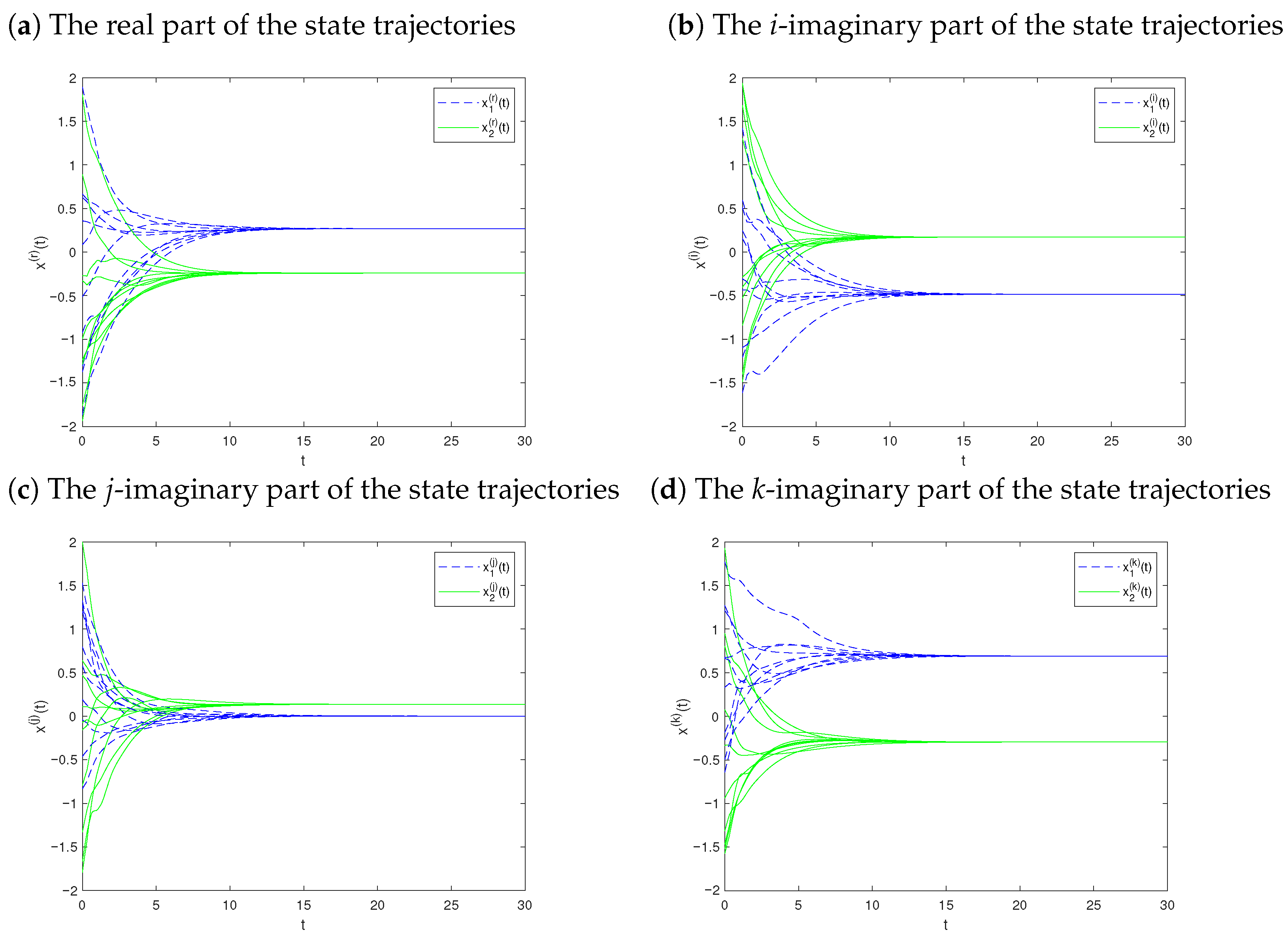
By employing the MATLAB Quaternion Toolbox, we perform numerical simulation of the proposed QVNNs. Figure 1a–d depict the four components of the state trajectories, i.e., the real part, the i-imaginary part, the j-imaginary part, and the k-imaginary part, respectively, where the initial conditions are chosen as 10 random constant quaternion-valued vectors.As can be seen from the figure, although the initial values are randomly distributed, all the state components eventually converge to the steady-state values around the 15th second. This convergence behavior is in perfect agreement with the theoretical prediction of Theorem 2, and provides an intuitive verification of the effectiveness of the obtained LMI conditions in ensuring global robust stability.

Remark 4.

In order to verify the effectiveness and scalability of the proposed method in a larger-scale network, we next consider QVNN (1) with $n=3$, and the parameter values are as follows:

$$\stackrel{\vee }{A}=\left(\begin{array}{ccc}0.7& 0& 0\\ 0& 0.75& 0\\ 0& 0& 0.8\end{array}\right),\stackrel{\wedge }{A}=\left(\begin{array}{ccc}0.8& 0& 0\\ 0& 0.85& 0\\ 0& 0& 0.9\end{array}\right),L=\left(\begin{array}{ccc}0.1& 0& 0\\ 0& 0.1& 0\\ 0& 0& 0.1\end{array}\right),$$

$$\stackrel{\vee }{B}={\left({\stackrel{\vee }{b}}_{ij}\right)}_{3\times 3},\stackrel{\wedge }{B}={\left({\stackrel{\wedge }{b}}_{ij}\right)}_{3\times 3},\stackrel{\vee }{C}={\left({\stackrel{\vee }{c}}_{ij}\right)}_{3\times 3},\stackrel{\wedge }{C}={\left({\stackrel{\wedge }{c}}_{ij}\right)}_{3\times 3},$$

$$\delta =0.05,\tau =0.1,h=0.3,f\left(x\left(t\right)\right)={\displaystyle \frac{0.8}{1+exp\left(x\right(t\left)\right)}}.$$

where

$$\begin{array}{ccccc}& {\stackrel{\vee }{b}}_{11}=-0.0680-0.0544i-0.0408j-0.0272k,\hfill & & {\stackrel{\vee }{b}}_{12}=-0.0340-0.0272i-0.0204j-0.0136k,\hfill & \\ & {\stackrel{\vee }{b}}_{13}=-0.0204-0.0163i-0.0122j-0.0082k,\hfill & & {\stackrel{\vee }{b}}_{21}=-0.0340-0.0272i-0.0204j-0.0136k,\hfill & \\ & {\stackrel{\vee }{b}}_{22}=-0.0680-0.0544i-0.0408j-0.0272k,\hfill & & {\stackrel{\vee }{b}}_{23}=-0.0272-0.0218i-0.0163j-0.0109k,\hfill & \\ & {\stackrel{\vee }{b}}_{31}=-0.0204-0.0163i-0.0122j-0.0082k,\hfill & & {\stackrel{\vee }{b}}_{32}=-0.0272-0.0218i-0.0163j-0.0109k,\hfill & \\ & {\stackrel{\vee }{b}}_{33}=-0.0680-0.0544i-0.0408j-0.0272k,\hfill & & {\stackrel{\vee }{c}}_{11}=-0.0544-0.0435i-0.0326j-0.0218k,\hfill & \\ & {\stackrel{\vee }{c}}_{12}=-0.0204-0.0163i-0.0122j-0.0082k,\hfill & & {\stackrel{\vee }{c}}_{13}=-0.0136-0.0109i-0.0082j-0.0054k,\hfill & \\ & {\stackrel{\vee }{c}}_{21}=-0.0204-0.0163i-0.0122j-0.0082k,\hfill & & {\stackrel{\vee }{c}}_{22}=-0.0544-0.0435i-0.0326j-0.0218k,\hfill & \\ & {\stackrel{\vee }{c}}_{23}=-0.0204-0.0163i-0.0122j-0.0082k,\hfill & & {\stackrel{\vee }{c}}_{31}=-0.0136-0.0109i-0.0082j-0.0054k,\hfill & \\ & {\stackrel{\vee }{c}}_{32}=-0.0204-0.0163i-0.0122j-0.0082k,\hfill & & {\stackrel{\vee }{c}}_{33}=-0.0544-0.0435i-0.0326j-0.0218k,\hfill & \\ & {\stackrel{\vee }{d}}_{11}=-0.0136-0.0109i-0.0082j-0.0054k,\hfill & & {\stackrel{\vee }{d}}_{12}=-0.0068-0.0054i-0.0041j-0.0027k,\hfill & \\ & {\stackrel{\vee }{d}}_{13}=-0.0034-0.0027i-0.0020j-0.0014k,\hfill & & {\stackrel{\vee }{d}}_{21}=-0.0068-0.0054i-0.0041j-0.0027k,\hfill & \\ & {\stackrel{\vee }{d}}_{22}=-0.0136-0.0109i-0.0082j-0.0054k,\hfill & & {\stackrel{\vee }{d}}_{23}=-0.0068-0.0054i-0.0041j-0.0027k,\hfill & \\ & {\stackrel{\vee }{d}}_{31}=-0.0034-0.0027i-0.0020j-0.0014k,\hfill & & {\stackrel{\vee }{d}}_{32}=-0.0068-0.0054i-0.0041j-0.0027k,\hfill & \\ & {\stackrel{\vee }{d}}_{33}=-0.0136-0.0109i-0.0082j-0.0054k,\hfill & & {\stackrel{\wedge }{b}}_{11}=0.0272+0.0544i+0.0680j+0.0408k,\hfill & \\ & {\stackrel{\wedge }{b}}_{12}=0.0136+0.0272i+0.0340j+0.0204k,\hfill & & {\stackrel{\wedge }{b}}_{13}=0.0082+0.0163i+0.0204j+0.0122k,\hfill & \\ & {\stackrel{\wedge }{b}}_{21}=0.0136+0.0272i+0.0340j+0.0204k,\hfill & & {\stackrel{\wedge }{b}}_{22}=0.0272+0.0544i+0.0680j+0.0408k,\hfill & \\ & {\stackrel{\wedge }{b}}_{23}=0.0109+0.0218i+0.0272j+0.0163k,\hfill & & {\stackrel{\wedge }{b}}_{31}=0.0082+0.0163i+0.0204j+0.0122k,\hfill & \\ & {\stackrel{\wedge }{b}}_{32}=0.0109+0.0218i+0.0272j+0.0163k,\hfill & & {\stackrel{\wedge }{b}}_{33}=0.0272+0.0544i+0.0680j+0.0408k,\hfill & \\ & {\stackrel{\wedge }{c}}_{11}=0.0218+0.0435i+0.0544j+0.0326k,\hfill & & {\stackrel{\wedge }{c}}_{12}=0.0082+0.0163i+0.0204j+0.0122k,\hfill & \\ & {\stackrel{\wedge }{c}}_{13}=0.0054+0.0109i+0.0136j+0.0082k,\hfill & & {\stackrel{\wedge }{c}}_{21}=0.0082+0.0163i+0.0204j+0.0122k,\hfill & \\ & {\stackrel{\wedge }{c}}_{22}=0.0218+0.0435i+0.0544j+0.0326k,\hfill & & {\stackrel{\wedge }{c}}_{23}=0.0082+0.0163i+0.0204j+0.0122k,\hfill & \\ & {\stackrel{\wedge }{c}}_{31}=0.0054+0.0109i+0.0136j+0.0082k,\hfill & & {\stackrel{\wedge }{c}}_{32}=0.0082+0.0163i+0.0204j+0.0122k,\hfill & \\ & {\stackrel{\wedge }{c}}_{33}=0.0218+0.0435i+0.0544j+0.0326k,\hfill & & {\stackrel{\wedge }{d}}_{11}=0.0054+0.0109i+0.0136j+0.0082k,\hfill & \\ & {\stackrel{\wedge }{d}}_{12}=0.0027+0.0054i+0.0068j+0.0041k,\hfill & & {\stackrel{\wedge }{d}}_{13}=0.0014+0.0027i+0.0034j+0.0020k,\hfill & \\ & {\stackrel{\wedge }{d}}_{21}=0.0027+0.0054i+0.0068j+0.0041k,\hfill & & {\stackrel{\wedge }{d}}_{22}=0.0054+0.0109i+0.0136j+0.0082k,\hfill & \\ & {\stackrel{\wedge }{d}}_{23}=0.0027+0.0054i+0.0068j+0.0041k,\hfill & & {\stackrel{\wedge }{d}}_{31}=0.0014+0.0027i+0.0034j+0.0020k,\hfill & \\ & {\stackrel{\wedge }{d}}_{32}=0.0027+0.0054i+0.0068j+0.0041k,\hfill & & {\stackrel{\wedge }{d}}_{33}=0.0054+0.0109i+0.0136j+0.0082k.\hfill \end{array}$$

With the above information, we get the following matrices:

$$\begin{array}{cccc}\hfill \tilde{B}& =\left(\begin{array}{ccc}0.1& 0.05& 0.03\\ 0.05& 0.1& 0.04\\ 0.03& 0.04& 0.1\end{array}\right),\tilde{C}\hfill & \hfill =\left(\begin{array}{ccc}0.08& 0.03& 0.02\\ 0.03& 0.08& 0.03\\ 0.02& 0.03& 0.08\end{array}\right),\tilde{D}& =\left(\begin{array}{ccc}0.02& 0.01& 0.05\\ 0.01& 0.02& 0.01\\ 0.005& 0.01& 0.02\end{array}\right).\hfill \end{array}$$

By employing the LMI toolbox in MATLAB, LMI (10) in Theorem 2 has a feasible solution as follows:

$$\begin{array}{cc}\hfill & Q_1=\left(\begin{array}{ccc}1.1867& 0& 0\\ 0& 1.1867& 0\\ 0& 0& 1.1867\end{array}\right),Q_2=\left(\begin{array}{ccc}0.4346& 0& 0\\ 0& 0.4346& 0\\ 0& 0& 0.4346\end{array}\right),\hfill \\ \hfill & Q_3=\left(\begin{array}{ccc}1.6988& 0& 0\\ 0& 1.6988& 0\\ 0& 0& 1.6988\end{array}\right),Q_4=\left(\begin{array}{ccc}0.3967& 0& 0\\ 0& 0.3967& 0\\ 0& 0& 0.3967\end{array}\right),\hfill \\ \hfill & Q_5=\left(\begin{array}{ccc}0.7043& 0& 0\\ 0& 0.7043& 0\\ 0& 0& 0.7043\end{array}\right),Q_6=\left(\begin{array}{ccc}0.1254& 0& 0\\ 0& 0.1254& 0\\ 0& 0& 0.1254\end{array}\right),\hfill \\ \hfill & Q_7=\left(\begin{array}{ccc}0.8618& 0& 0\\ 0& 0.8618& 0\\ 0& 0& 0.8618\end{array}\right),P_1=\left(\begin{array}{ccc}0.4875& 0& 0\\ 0& 0.4875& 0\\ 0& 0& 0.4875\end{array}\right),\hfill \\ \hfill & P_2=\left(\begin{array}{ccc}0.3026& 0& 0\\ 0& 0.3026& 0\\ 0& 0& 0.3026\end{array}\right),R_1=\left(\begin{array}{ccc}1.4700& 0& 0\\ 0& 1.4700& 0\\ 0& 0& 1.4700\end{array}\right),\hfill \\ \hfill & R_2=\left(\begin{array}{ccc}0.9104& 0& 0\\ 0& 0.9104& 0\\ 0& 0& 0.9104\end{array}\right).\hfill \end{array}$$

By Theorems 1 and 2, the equilibrium point of QVNN (1) exists uniquely and this equilibrium point is globally robust stable.

Remark 5.

Here, we provide an explanation for the exponential function in the activation function of QVNN (1). The exponential function of a quaternion q is defined as $exp\left(q\right)=exp(R)\left(cos\left(\left|I\right|\right)+{\displaystyle \frac{I}{\left|I\right|}}sin\left(\left|I\right|\right)\right)$, where $R=Re\left(q\right),I=Im\left(q\right)$ (used in numerical simulation calculations). For more details about this function, readers can refer to [43]. Moreover, the activation function of QVNN (1) is the Sigmoid function, which satisfies the Lipschitz condition. The Lipschitz condition is widely present in various common functions. Particularly, the activation functions commonly used in neural networks (such as Sigmoid, tanh, ReLU, and Leaky ReLU) all satisfy the global or local Lipschitz condition. The proof is as follows:

For any quaternion $q=a+bi+cj+dk\in \mathbb{H}$, and where the activation function is implemented in a component-wise manner, we have: $f\left(q\right)=\sigma \left(a\right)+\sigma \left(b\right)i+\sigma \left(c\right)j+\sigma \left(d\right)k$, where $\sigma \left(t\right)={\displaystyle \frac{0.8}{1+e^{-t}}}$ represents the real-valued Sigmoid function. The derivative of the real function $\sigma \left(t\right)$ satisfies $|{\sigma }^{\prime }\left(t\right)|\le 0.2$. Hence, for any real or imaginary components, we have $|\sigma \left(t_1\right)-\sigma \left(t_2\right)| \le 0.2|t_1-t_2|.$ For any two quaternions $q_1=a_1+b_{1}i+c_{1}j+d_{1}k$ and $q_2=a_2+b_{2}i+c_{2}j+d_{2}k$, we have $|f\left(q_1\right)-f\left(q_2\right){|}^2=|\sigma \left(a_1\right)-\sigma \left(a_2\right){|}^2+|\sigma \left(b_1\right)-\sigma \left(b_2\right){|}^2+|\sigma \left(c_1\right)-\sigma \left(c_2\right){|}^2+|\sigma \left(d_1\right)-\sigma \left(d_2\right){|}^2\le {\left(0.2\right)}^2\left[|a_1-a_2{|}^2+|b_1-b_2{|}^2+|c_1-c_2{|}^2+{|d_1-d_2|}^2\right]={\left(0.2\right)}^2{|q_1-q_2|}^2.$ Therefore, $|f\left(q_1\right)-f\left(q_2\right)|\le 0.2|q_1-q_2|,$ which satisfies Hypothesis 2 with Lipschitz constant $L=0.2$.

Example 2.

If choosing $D=0$, as in Example 1, then QVNN (1) is converted to QVNN (25), and solutions of LMI (26) can be resolved as:

$$\begin{array}{cc}\hfill & P_1=\left(\begin{array}{cc}3.3600& 0\\ 0& 3.3600\end{array}\right),P_2=\left(\begin{array}{cc}0.9130& 0\\ 0& 0.9130\end{array}\right),Q_1=\left(\begin{array}{cc}56.8817& 0\\ 0& 56.8817\end{array}\right),\hfill \\ \hfill & Q_2=\left(\begin{array}{cc}2.0088& 0\\ 0& 2.0088\end{array}\right),Q_3=\left(\begin{array}{cc}263.6965& 0\\ 0& 263.6965\end{array}\right),Q_4=\left(\begin{array}{cc}12.0705& 0\\ 0& 12.0705\end{array}\right),\hfill \\ \hfill & Q_5=\left(\begin{array}{cc}22.7311& 0\\ 0& 22.7311\end{array}\right),Q_6=\left(\begin{array}{cc}0.3323& 0\\ 0& 0.3323\end{array}\right),Q_7=\left(\begin{array}{cc}106.8031& 0\\ 0& 106.8031\end{array}\right),\hfill \\ \hfill & R_1=\left(\begin{array}{cc}320.7273& 0\\ 0& 320.7273\end{array}\right),R_2=\left(\begin{array}{cc}285.0020& 0\\ 0& 285.0020\end{array}\right).\hfill \end{array}$$

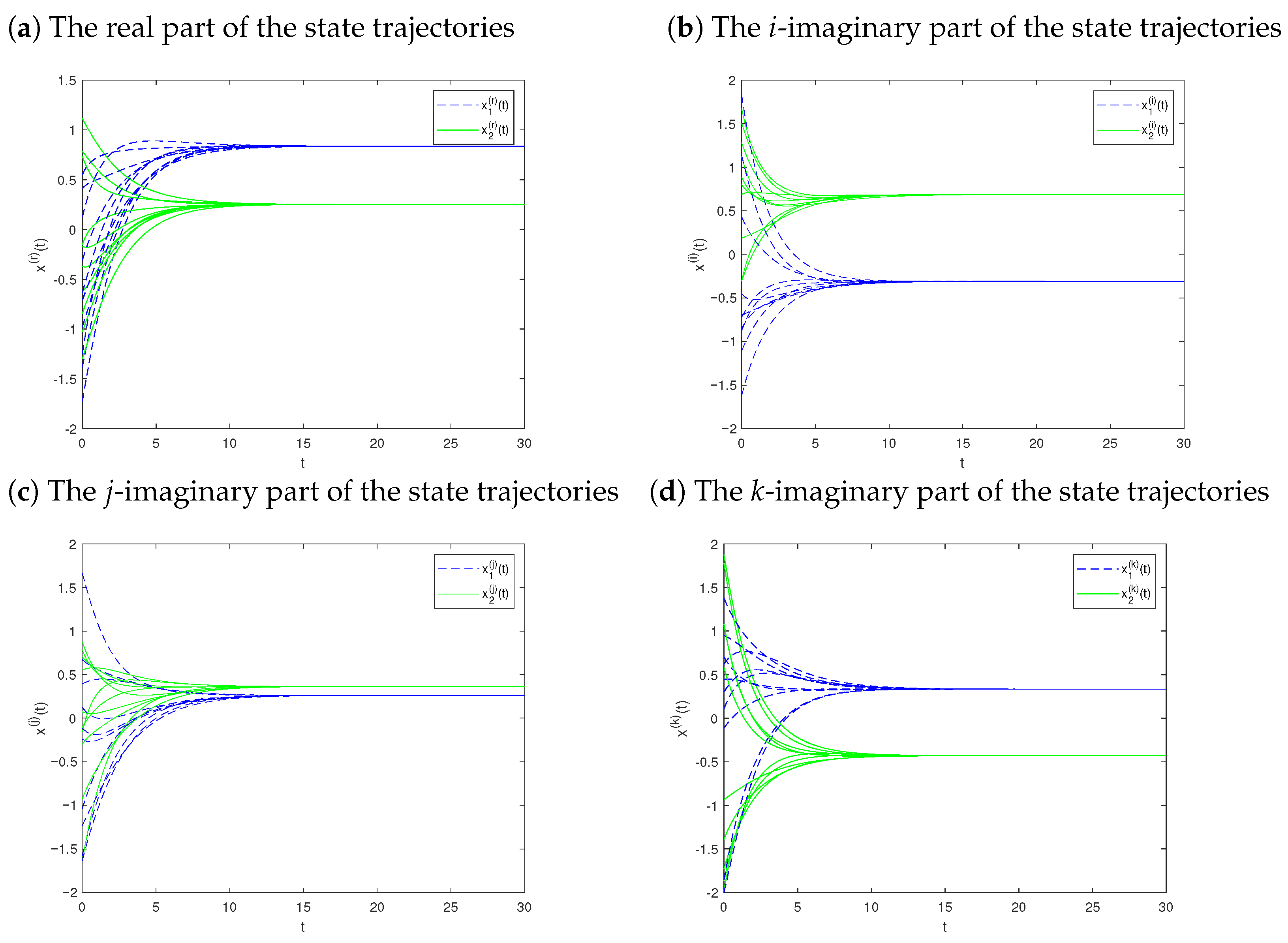
By Theorems 1 and 2, the equilibrium point of QVNN (25) exists uniquely, and this equilibrium point is globally robust stable. And we give Figure 2, which describes each of the four parts of the system state by simulating with 10 random constant quaternion values. As can be seen from Figure 2, the trajectories of each component in the figure all converge to a stable state around the 15th second.

Figure 2a–d depicts the state evolution curves of QVNNs (25) under the same parameter settings (with $D=0$), which also include the four components of the quaternion. This model is a special case without neutral delay, and its global robust stability is guaranteed by LMI (26) in the Corollary 1. The trajectories of each component in the figure all exhibit good convergence characteristics, further verifying the validity of the lemma results. Compared with Figure 1, the convergence speed of the system in Figure 2 is slightly different, reflecting the influence of the neutral delay term on the dynamic behavior.

Remark 6.

Examples 1 and 2 respectively verified the validity of Theorem 2 under the conditions of neutral delay and without neutral delay. From the numerical results, it can be seen that when the network size is $n=2$, the feasible solution size of the LMI in Example 1 is larger, and the numerical values of most weighting matrices are significantly higher than those in Example 2. This indicates that the introduction of neutral time delay makes the stability conditions of the system more stringent, and stronger feedback gains are required to ensure the robust stability of the system. Both sets of parameters can meet the proposed stability conditions, indicating that the LMI criterion established in this paper has good adaptability to different system structures. Moreover, the comparative analysis also reveals a positive correlation between the conservatism of the theoretical conditions and the complexity of the system: the more types of time delays and the more complex the system structure, the larger the numerical value of the LMI feasible solution, and the conservatism of the stability conditions is also correspondingly enhanced. This result provides useful insights for further reducing conservatism and optimizing control design.

To verify the low conservativeness advantage of the proposed method, this paper selected references [18,44] as the comparison benchmarks. Using the MATLAB LMI toolbox, the three strategies were numerically solved. Based on the parameters provided in Example 1 of this article, the conservativeness and computational complexity of each method were evaluated by comparing the upper limit of the maximum allowable delay with the number of LMI variables. The results are shown in

Table 2. Upper bound comparison of the time delay.

Method	${\mathit{\delta }}_{max}$	${\mathit{\tau }}_{max}$	${\mathit{h}}_{max}/{\mathit{\rho }}_{max}$	Number of LMI Variables
This paper	1.26	0.75	0.60	11
Paper [44]	1.00	–	0.50	9
Paper [18]	0.45	0.55	0.55	9

$\rho$ represents the types of time delays that have not been studied in the previous literature or have not been directly compared in this paper.

.

The one-dimensional search is conducted using the control variable method. Taking the discrete delay $\tau$ as an example, the process is as follows: fix the leakage delay $\delta$ and the neutral delay h as typical values, and gradually increase the value of $\tau$. For each $\tau$ value, call the LMI solver in MATLAB to determine whether there exists a set of feasible positive definite matrix solutions for the corresponding LMI system. If it can be solved, the system is stable at that $\tau$ value, and we record the $\tau$ values that meet the conditions until the critical point that makes the LMI have no solution is found. The previous feasible value before this critical point is the current maximum allowable discrete delay ${\tau }_{max}$ under the current setting. This process is repeated for $\delta$ and h.

Table 2 shows that the method proposed in this paper outperforms those in the comparison literature in terms of the maximum allowable upper bound of leakage delay (${\delta }_{max}\approx 1.26$) and the maximum allowable upper bound of discrete delay (${\tau }_{max}\approx 0.75$), demonstrating stronger robustness. Although the number of variables in the LMI is slightly larger, the allowable time delay boundary for the system is significantly increased. Moreover, by comprehensively considering more practical factors, this research offers broader applicability and distinct advantages.

The leakage delay $\delta$, discrete delay $\tau$, and neutral delay h all appear in the integral terms and derivative estimation of the Lyapunov functional. From the term ${\delta }^2{Q}_3$ in $V_3$ and the integral inequality in Lemma 5, it can be seen that larger delay values impose higher requirements on the weighting matrices $Q_3$, $Q_4$, and $Q_7$ in the LMI, and thus the feasibility of the conditions decreases accordingly. To illustrate this effect intuitively,

Table 3. LMI feasibility analysis under different delay bounds.

Case	$\mathit{\delta }$	$\mathit{\tau }$	h	Feasibility
1	1.00	0.60	0.45	✓
2	1.26	0.75	0.60	✓
3	1.30	0.80	0.70	×
4	1.40	0.90	0.80	×

presents the numerical feasibility results of the LMI under different combinations of delay bounds. By gradually increasing the values of $\delta$, $\tau$, and h, we observe whether the LMI remains feasible. The results show that, under this set of parameters, the system is relatively sensitive to delays: when the delays exceed certain ranges (approximately $\delta =1.26$, $\tau =0.75$, and $h=0.60$), the LMI is no longer feasible, and the robust stability of the system cannot be guaranteed.

5. Conclusions

In this paper, the robust stability problem of QVNNs with leakage, discrete, and neutral time delays, as well as parameter uncertainties, is investigated by employing a direct quaternion approach. Without decomposing the QVNNs into real-valued or complex-valued systems, the existence and uniqueness of the equilibrium point are proved via the homogeneous mapping theorem. By constructing an appropriate Lyapunov–Krasovskii functional and utilizing quaternion modulus inequality techniques together with the LMI approach, sufficient conditions for the global robust stability of the system are derived. This paper for the first time incorporates three types of time delays and interval parameter uncertainties into a unified QVNNs analysis framework, filling the gap in existing research. By using the direct quaternion path, the quaternion algebra structure is fully retained, avoiding the conservatism and redundancy caused by decomposition. The established LMI conditions explicitly incorporate the uncertainty intervals of weights, enhancing the practicality and robustness of the theoretical results. Numerical simulations have verified the effectiveness and superiority of the proposed method. Furthermore, in order to further reduce conservatism and expand the application scope of the analysis methods, future research will draw on the ideas from reference [45] to explore a complementary integration strategy between decomposition methods and direct methods, and construct a more expressive analysis framework to support the stability analysis of large-scale systems. Furthermore, in the subsequent work, we will refer to the research in reference [46] and extend the current method to the random quaternion neural network, focusing on its random stability issue. Specifically, we will draw on the random differential equation model and stability analysis method established in this paper, combined with the Lyapunov function technique, to study the impact of random perturbations on the dynamic behavior of the neural network.

References

1. Barrachina, J.A.; Ren, C.; Morisseau, C.; Vieillard, G.; Ovarlez, J.P. Comparison between equivalent architectures of complex-valued and real-valued neural networks-Application on polarimetric SAR image segmentation. J. Signal Process. Syst. 2023, 95, 57–66. [Google Scholar] [CrossRef]
2. Kaveh, A. Applications of artificial neural networks and machine learning in civil engineering. Stud. Comput. Intell. 2024, 1168, 472. [Google Scholar]
3. Li, H.L.; Jiang, H.; Cao, J. Global synchronization of fractional-order quaternion-valued neural networks with leakage and discrete delays. Neurocomputing 2020, 385, 211–219. [Google Scholar] [CrossRef]
4. Paul, V.S.; Nelson, P.A. Efficient design of complex-valued neural networks with application to the classification of transient acoustic signals. J. Acoust. Soc. Am. 2024, 156, 1099–1110. [Google Scholar] [CrossRef]
5. Xie, X.; Li, C.; Guan, T.; Zheng, Y.; Wu, X. A novel complex-valued convolutional network for real-world single image dehazing. J. Vis. Commun. Image Represent. 2023, 97, 103984. [Google Scholar] [CrossRef]
6. Zeng, Z.; Sun, J.; Han, Z.; Hong, W. SAR automatic target recognition method based on multi-stream complex-valued networks. IEEE Trans. Geosci. Remote Sens. 2022, 60, 1–18. [Google Scholar] [CrossRef]
7. Yin, Q.; Wang, J.; Luo, X.; Zhai, J.; Jha, S.K.; Shi, Y.Q. Quaternion convolutional neural network for color image classification and forensics. IEEE Access 2019, 7, 20293–20301. [Google Scholar] [CrossRef]
8. Neshat, M.; Nezhad, M.M.; Mirjalili, S.; Piras, G.; Garcia, D.A. Quaternion convolutional long short-term memory neural model with an adaptive decomposition method for wind speed forecasting: North aegean islands case studies. Energy Convers. Manag. 2022, 259, 115590. [Google Scholar] [CrossRef]
9. Chen, B.; Shu, H.; Zhang, H.; Chen, G.; Toumoulin, C.; Dillenseger, J.L.; Luo, L.M. Quaternion Zernike moments and their invariants for color image analysis and object recognition. Signal Process. 2012, 92, 308–318. [Google Scholar] [CrossRef]
10. Zhou, H.; Zhang, X.; Zhang, C.; Ma, Q. Quaternion convolutional neural networks for hyperspectral image classification. Eng. Appl. Artif. Intell. 2023, 123, 106234. [Google Scholar] [CrossRef]
11. Frants, V.; Agaian, S.; Panetta, K. QCNN-H: Single-image dehazing using quaternion neural networks. IEEE Trans. Cybern. 2023, 53, 5448–5458. [Google Scholar] [CrossRef]
12. Yuan, H.; Zhu, Q. Stabilities of delay stochastic McKean-Vlasov equations in the G-framework. Sci. China Inf. Sci. 2025, 68, 1–23. [Google Scholar] [CrossRef]
13. Xu, H.; Zhu, Q.; Zheng, W.X. Exponential stability of stochastic nonlinear delay systems subject to multiple periodic impulses. IEEE Trans. Autom. Control 2023, 69, 2621–2628. [Google Scholar] [CrossRef]
14. Song, Q.; Wu, Q.; Liu, Y. Stabilization of chaotic quaternion-valued neutral-type neural networks via sampled-data control with two-sided looped functional approach. Nonlinear Anal. Model. Control 2024, 29, 1144–1160. [Google Scholar] [CrossRef]
15. Song, Q. Exponential stability of recurrent neural networks with both time-varying delays and general activation functions via LMI approach. Neurocomputing 2008, 71, 2823–2830. [Google Scholar] [CrossRef]
16. Tu, Z.; Cao, J.; Alsaedi, A.; Hayat, T. Global dissipativity analysis for delayed quaternion-valued neural networks. Neural Netw. 2017, 89, 97–104. [Google Scholar] [CrossRef]
17. Banu, L.J.; Balasubramaniam, P. Robust stability analysis for discrete-time neural networks with time-varying leakage delays and random parameter uncertainties. Neurocomputing 2016, 179, 126–134. [Google Scholar] [CrossRef]
18. Tu, Z.; Zhao, Y.; Ding, N.; Feng, Y.; Zhang, W. Stability analysis of quaternion-valued neural networks with both discrete and distributed delays. Appl. Math. Comput. 2019, 343, 342–353. [Google Scholar] [CrossRef]
19. Chen, Y.; Zhang, X.; Xue, Y. Global exponential synchronization of high-order quaternion Hopfield neural networks with unbounded distributed delays and time-varying discrete delays. Math. Comput. Simul. 2022, 193, 173–189. [Google Scholar] [CrossRef]
20. Naik, P.A.; Eskandari, Z. Nonlinear dynamics of a three-dimensional discrete-time delay neural network. Int. J. Biomath. 2024, 17, 2350057. [Google Scholar] [CrossRef]
21. Yan, H.; Qiao, Y.; Duan, L.; Miao, J. New results of quasi-projective synchronization for fractional-order complex-valued neural networks with leakage and discrete delays. Chaos Solitons Fractals 2022, 159, 112121. [Google Scholar] [CrossRef]
22. Kong, F.; Zhu, Q. Finite-time stabilization of discontinuous fuzzy neutral-type neural networks with D operator and multiple time-varying delays. Fuzzy Sets Syst. 2022, 449, 32–55. [Google Scholar] [CrossRef]
23. Zhang, Z.; Zhang, X.; Yu, T. Global exponential stability of neutral-type Cohen–Grossberg neural networks with multiple time-varying neutral and discrete delays. Neurocomputing 2022, 490, 124–131. [Google Scholar] [CrossRef]
24. Arik, S. New criteria for stability of neutral-type neural networks with multiple time delays. IEEE Trans. Neural Netw. Learn. Syst. 2019, 31, 1504–1513. [Google Scholar] [CrossRef]
25. Xu, C.; Liu, Z.; Aouiti, C.; Li, P.; Yao, L.; Yan, J. New exploration on bifurcation for fractional-order quaternion-valued neural networks involving leakage delays. Cogn. Neurodyn. 2022, 16, 1233–1248. [Google Scholar] [CrossRef]
26. Zhao, M.; Li, H.L.; Zhang, L.; Hu, C.; Jiang, H. Quasi-synchronization of discrete-time fractional-order quaternion-valued memristive neural networks with time delays and uncertain parameters. Appl. Math. Comput. 2023, 453, 128095. [Google Scholar] [CrossRef]
27. Zhang, T.; He, W. Global robust stability of fuzzy cellular neural networks with parameter uncertainties. AIMS Math. 2024, 9, 8063–8078. [Google Scholar] [CrossRef]
28. Bin, L.; Liu, X.Z.; Liao, X.X. Robust H-stability of Hopfield neural networks with impulsive effects and design of impulsive controllers. Control Theory Appl. 2003, 20, 168–172. [Google Scholar]
29. Sakthivel, R.; Mathiyalagan, K.; Marshal Anthoni, S. Robust H control for uncertain discrete-time stochastic neural networks with time-varying delays. IET Control Theory Appl. 2012, 6, 1220–1228. [Google Scholar] [CrossRef]
30. Huang, H.; Feng, G.; Sun, Y. Robust synchronization of chaotic systems subject to parameter uncertainties. Chaos Interdiscip. J. Nonlinear Sci. 2009, 19, 033128. [Google Scholar] [CrossRef] [PubMed]
31. Liao, X.; Wang, J.; Cao, J. Global and robust stability of interval Hopfield neural networks with time-varying delays. Int. J. Neural Syst. 2003, 13, 171–182. [Google Scholar] [CrossRef] [PubMed]
32. Pan, J.; Pan, Z. Novel robust stability criteria for uncertain parameter quaternionic neural networks with mixed delays: Whole quaternionic method. Appl. Math. Comput. 2021, 407, 126326. [Google Scholar] [CrossRef]
33. Gunasekaran, N.; Thoiyab, N.M.; Zhu, Q.; Cao, J.; Muruganantham, P. New global asymptotic robust stability of dynamical delayed neural networks via intervalized interconnection matrices. IEEE Trans. Cybern. 2021, 52, 11794–11804. [Google Scholar] [CrossRef]
34. Wang, X.; Yu, J.; Li, C.; Wang, H.; Huang, T.; Huang, J. Robust stability of stochastic fuzzy delayed neural networks with impulsive time window. Neural Netw. 2015, 67, 84–91. [Google Scholar] [CrossRef]
35. Chanthorn, P.; Rajchakit, G.; Humphries, U.; Kaewmesri, P.; Sriraman, R.; Lim, C.P. A delay-dividing approach to robust stability of uncertain stochastic complex-valued hopfield delayed neural networks. Symmetry 2020, 12, 683. [Google Scholar] [CrossRef]
36. Ali, M.S.; Gunasekaran, N.; Rani, M.E. Robust stability of Hopfield delayed neural networks via an augmented LK functional. Neurocomputing 2017, 234, 198–204. [Google Scholar] [CrossRef]
37. Li, R.; Gao, X.; Cao, J.; Zhang, K. Dissipativity and exponential state estimation for quaternion-valued memristive neural networks. Neurocomputing 2019, 363, 236–245. [Google Scholar] [CrossRef]
38. Liu, Y.; Zhang, D.; Lu, J. Global exponential stability for quaternion-valued recurrent neural networks with time-varying delays. Nonlinear Dyn. 2017, 87, 553–565. [Google Scholar] [CrossRef]
39. Li, Y.; Qin, J. Existence and global exponential stability of periodic solutions for quaternion-valued cellular neural networks with time-varying delays. Neurocomputing 2018, 292, 91–103. [Google Scholar] [CrossRef]
40. Chen, X.; Li, Z.; Song, Q.; Hu, J.; Tan, Y. Robust stability analysis of quaternion-valued neural networks with time delays and parameter uncertainties. Neural Netw. 2017, 91, 55–65. [Google Scholar] [CrossRef] [PubMed]
41. Fang, T.; Sun, J. Stability of complex-valued recurrent neural networks with time-delays. IEEE Trans. Neural Netw. Learn. Syst. 2014, 25, 1709–1713. [Google Scholar] [CrossRef]
42. Boyd, S.; El Ghaoui, L.; Feron, E.; Balakrishnan, V. Linear Matrix Inequalities in System and Control Theory; SIAM: Philadelphia, PA, USA, 1994. [Google Scholar]
43. Kuipers, J.B. Quaternions and Rotation Sequences: A Primer with Applications to Orbits, Aerospace, and Virtual Reality; Princeton University Press: Princeton, NJ, USA, 1999. [Google Scholar]
44. Song, Q.; Yang, L.; Liu, Y.; Alsaadi, F.E. Stability of quaternion-valued neutral-type neural networks with leakage delay and proportional delays. Neurocomputing 2023, 521, 191–198. [Google Scholar] [CrossRef]
45. Liu, Y.; Zhang, D.; Lou, J.; Lu, J.; Cao, J. Stability analysis of quaternion-valued neural networks: Decomposition and direct approaches. IEEE Trans. Neural Netw. Learn. Syst. 2017, 29, 4201–4211. [Google Scholar] [CrossRef] [PubMed]
46. Waezizadeh, T.; Mehrpooya, A. A stochastic model for dynamics of two populations and its stability. In Proceedings of the 47th Annual Iranian Mathematics Conference (AIMC47), Karaj, Iran, 28–31 August 2016. [Google Scholar]
Figure 1. The simulation results of x ( r ) ( t ) , x ( i ) ( t ) , x ( j ) ( t ) and x ( k ) ( t ) of QVNN (1) with 10 random initial conditions.
Axioms 15 00249 g001
Figure 2. The simulation results of x ( r ) ( t ) , x ( i ) ( t ) , x ( j ) ( t ) and x ( k ) ( t ) of QVNN (25) with 10 random initial conditions.
Axioms 15 00249 g002