Structured Over-Relaxed Monotone FISTA for Linear Inverse Problems in Image Restoration

Abstract

In this paper, we propose an efficient numerical algorithm for solving large-scale ill-posed linear inverse problems encountered in image restoration. To boost computational efficiency, we extend the structured fast iterative shrinkage-thresholding algorithm (sFISTA) for addressing the corresponding $l_1$-regularized minimization problem, and further introduce the over-relaxation technique to accelerate the algorithm. The proposed algorithm is termed structured over-relaxed monotone FISTA (sOMFISTA). The convergence analysis of sOMFISTA is also conducted. The algorithmic framework of sOMFISTA is universally applicable to any non-smooth convex regularization term, exhibiting remarkable flexibility. Extensive numerical experiments are carried out to systematically validate the superiority in efficiency and performance of the proposed sOMFISTA.

1. Introduction

Linear inverse problems arise in a wide range of applications such as signal and image processing, statistics, and compressed sensing, to name just a few. Mathematically, a linear inverse problem can be modeled as

$$\mathbf{b}=\mathbf{Ax}+\mathbf{e},$$

(1)

where each term is explicitly defined in the context of image restoration as follows:

• $\mathbf{x}\in {\mathbb{R}}^N$: The unknown vectorized form of the true underlying image (with $N=m\times n$ for an $m\times n$ pixel image), which is the target image we aim to recover.
• $\mathbf{A}\in {\mathbb{R}}^{N\times N}$: A linear transformation matrix that characterizes the degradation process of the image. In image deblurring, $\mathbf{A}$ is constructed based on the point spread function (PSF) of the blur kernel, and its structure is often in block Toeplitz or Kronecker product form to reflect the spatial correlation of the image.
• $\mathbf{b}\in {\mathbb{R}}^N$: The observed image vector obtained from real-world measurements, which corresponds to the vectorized form of the blurry/noisy image captured by imaging devices.
• $\mathbf{e}\in {\mathbb{R}}^N$: An unknown additive noise vector introduced during image acquisition or transmission.

In image reconstruction applications, the matrix $\mathbf{A}$ is ill-conditioned, which poses challenges during estimation processes. The fundamental approach to the (1) involves formulating an objective function that encompasses regularization and fidelity terms:

$$\underset{\mathbf{x}}{min} {\displaystyle \frac{1}{2}}{\parallel \mathbf{Ax}-\mathbf{b}\parallel }_2^2+\lambda R\left(\mathbf{x}\right),$$

where $\lambda >0$ is a regularization parameter. Widely used regularization terms include Tikhonov regularization [1], $l_1$ regularization [2], total variational (TV) regularization [3], and so on. The choice of an appropriate regularization scheme has a direct influence on both the precision of the reconstructed results and the computational complexity of the optimization procedure. Tikhonov regularization, which is based on the $l_2$ norm, tends to over-smooth image details and edges, often leading to over-smoothed solutions that fail to preserve fine structures and textural information. Total variation (TV) regularization, while effective in maintaining sharp edges, frequently introduces staircase effects and may over-suppress small-scale features, resulting in visually unnatural and overly piecewise-constant images. By contrast, $l_1$ regularization offers a more balanced framework that can effectively recover sparse image components while avoiding excessive smoothing and artificial artifacts, making it a more suitable choice for robust and high-fidelity image restoration. In this paper, $l_1$ regularization [2] is used, which is convex and non-smooth. Then the optimization model has the following form:

$$\underset{\mathbf{x}}{min} F\left(\mathbf{x}\right)={\displaystyle \frac{1}{2}}{\parallel \mathbf{Ax}-\mathbf{b}\parallel }_2^2+\lambda {\parallel \mathbf{x}\parallel }_1.$$

(2)

Numerous iterative-based algorithms have been proposed for solving problem (2), among which a class of algorithms based on the proximal method is very popular, including the iterative shrinkage-thresholding algorithm (ISTA) [4], fast iterative shrinkage-thresholding algorithm (FISTA) [5], monotone FISTA (MFISTA) [6], over-relaxed monotone FISTA (OMFISTA) [7], new over-relaxed monotone FISTA (OMFISTAv2) [8] and structured FISTA (sFISTA) [9]. ISTA is the simplest one, where each iteration only requires simple matrix-vector multiplication and a shrinkage/soft-threshold step. However, ISTA converges quite slowly. FISTA not only keeps the simplicity of ISTA but also improves the convergence rate significantly. However, it does not guarantee the monotonicity in objective function values. By comparing the objective function values at two points at each iteration, MFISTA overcomes the non-monotonicity of FISTA. Applying an over-relaxation technique, OMFISTA admits possibly better performance in a well-conditioned case. However, it is slower than MFISTA when $\mathbf{A}$ is ill-conditioned, which often occurs. In OMFISTAv2, a new parameter setting strategy is employed, which makes it faster than MFISTA when $\mathbf{A}$ is ill-conditioned or rank-deficient. All these algorithms based on the proximal method mentioned above are not suitable for parallel implementation. sFISTA leverages two hidden structures of the problem to make parallel implementation possible; however, its convergence analysis is not applicable for the non-smooth case.

Table 1. Comparison of related FISTA-type algorithms for image restoration.

Method	Idea	Rate	Monotone	Advantages	Limitations
ISTA [4]	Proximal gradient	$O(1/k)$	No	Simple	Slow
FISTA [5]	Nesterov acceleration	$O(1/k^2)$	No	Fast convergence	Non-monotone
MFISTA [5]	Monotone FISTA	$O(1/k^2)$	Yes	Stable decrease	Higher cost
OMFISTA [7]	Over-relaxation	$O(1/k^2)$	Yes	Faster in some cases	Parameter tuning
OMFISTAv2 [8]	Improved parameters	$O(1/k^2)$	Yes	Improved stability	Sequential
sFISTA [9]	Structured approach	$O(1/k^2)$	No	Parallelizable	Smooth case only
sOMFISTA [Our]	Structured + relaxation	$O(1/k^2)$	Yes	Faster execution	Approximation error

presents a concise comparison of the existing FISTA-type algorithms, highlighting their core ideas, convergence rates, and monotonicity, as well as their respective advantages and limitations.

The remaining sections are organized as follows. In Section 2, we give a short review of the class of iterative shrinkage algorithms. In Section 3, we first provide an overview of the sOMFISTA structure and subsequently derive the convergence analysis. Some numerical examples are presented in Section 4, followed by concluding remarks in Section 5.

In this paper, we propose a structured over-relaxed monotone FISTA (sOMFISTA) method for image restoration problems. The main contributions of this work are summarized as follows: (1) We incorporate the Kronecker product approximation of the blurring matrix and the over-relaxation technique into the monotone FISTA framework, yielding the sOMFISTA algorithm. This structure not only accelerates the convergence speed of MFISTA for ill-conditioned problems but also enables efficient parallel implementation. (2) The proposed sOMFISTA framework is flexible and general: it can handle the objective function with arbitrary convex non-smooth regularizers, which allows straightforward extensions to various non-smooth minimization models in image restoration. (3) We provide a rigorous convergence analysis for the sOMFISTA algorithm. The theoretical results are general enough to cover a wide class of convex non-smooth regularization terms, ensuring the stability and reliability of the proposed method in practical applications.

2. Iterative Shrinkage Algorithms

In this section, we give a short review on iterative shrinkage algorithms for the following general non-smooth optimization problem:

$$\underset{\mathbf{x}\in {\mathbb{R}}^n}{min} \{F\left(\mathbf{x}\right)=f\left(\mathbf{x}\right)+g\left(\mathbf{x}\right)\},$$

where $f:{\mathbb{R}}^n\to \mathbb{R}, g:\mathrm{dom}\to \mathbb{R}$ are convex functions and g is possibly non-smooth. For any $L>0$ and a given point $\mathbf{y}\in {\mathbb{R}}^n$, $f\left(\mathbf{x}\right)$ has a quadratic approximation:

$$q_L(\mathbf{x},\mathbf{y}):=f\left(\mathbf{y}\right)+\langle \nabla f\left(\mathbf{y}\right),\mathbf{x}-\mathbf{y}\rangle +{\displaystyle \frac{L}{2}}{\parallel \mathbf{x}-\mathbf{y}\parallel }_2^2.$$

Then the function $Q_L(\mathbf{x},\mathbf{y}):=q_L(\mathbf{x},\mathbf{y})+g\left(\mathbf{x}\right)$ has a unique minimizer:

$$P_L\left(\mathbf{y}\right):=\underset{\mathbf{x}\in {\mathbb{R}}^n}{argmin} Q_L(\mathbf{x},\mathbf{y}).$$

ISTA is an extension of the classical gradient method, whose convergence rate is $O\left({\displaystyle \frac{1}{k}}\right)$. The iterative scheme of the ISTA is as follows:

$${\mathbf{x}}_{k+1}=P_L\left({\mathbf{x}}_k\right),$$

where $L\ge L_{\nabla f}={\parallel {\mathbf{A}}^T\mathbf{A}\parallel }_2$ and $L_{\nabla f}$ being the Lipschitz constant of $\nabla f$. FISTA chooses an additional point $y_{k+1}$ as a linear combination of two previous iteration points, i.e.,

$${\mathbf{y}}_{k+1}={\mathbf{x}}_k+\left({\displaystyle \frac{t_k-1}{t_{k+1}}}\right)({\mathbf{x}}_k-{\mathbf{x}}_{k-1}),$$

where $t_{k+1}={\displaystyle \frac{1+\sqrt{1+4{t_k}^2}}{2}}$ with $t_1=1$ and ${\mathbf{y}}_1={\mathbf{x}}_0$. The next iteration point ${\mathbf{x}}_{k+1}$ is then set as the unique minimizer:

$${\mathbf{x}}_{k+1}=P_L\left({\mathbf{y}}_{k+1}\right).$$

FISTA preserves the computational simplicity and has a fast global convergence rate $O\left({\displaystyle \frac{1}{k^2}}\right)$. MFISTA maintains the convergence rate $O\left({\displaystyle \frac{1}{k^2}}\right)$, which produces a monotonically non-increasing sequence $\left\{F\left({\mathbf{x}}_k\right)\right\}$ via iterative steps

$${\mathbf{x}}_{k+1}=\underset{\mathbf{x}\in {\mathbb{R}}^n}{argmin} \left\{F\left(\mathbf{x}\right)\right|\mathbf{x}\in \{{\mathbf{x}}_k,{\mathbf{z}}_{k+1}\}\}.$$

In the equation above, ${\mathbf{z}}_{k+1}=P_L\left({\mathbf{y}}_{k+1}\right)$, where

$${\mathbf{y}}_{k+1}={\mathbf{x}}_k+\left({\displaystyle \frac{t_k}{t_{k+1}}}\right)({\mathbf{z}}_k-{\mathbf{x}}_k)+\left({\displaystyle \frac{t_k-1}{t_{k+1}}}\right)({\mathbf{x}}_k-{\mathbf{x}}_{k-1}).$$

OMFISTA also generates a monotonically non-increasing sequence $\left\{F\left({\mathbf{x}}_k\right)\right\}$ with the convergence rate $O\left({\displaystyle \frac{1}{k^2}}\right)$, where three additional parameters ${\lambda }_k,{\xi }_k$ and ${\eta }_k$ are introduced. Specifically, the iterative scheme of the OMFISTA is as follows:

$${\mathbf{x}}_{k+1}=\underset{\mathbf{x}\in {\mathbb{R}}^n}{argmin} \left\{F\left(\mathbf{x}\right)\right|\mathbf{x}\in \{{\mathbf{x}}_k,{\mathbf{x}}_k+{\lambda }_k({\mathbf{z}}_{k+1}-{\mathbf{x}}_k)\}\},$$

where ${\mathbf{z}}_{k+1}=P_{{\displaystyle \frac{1}{{\xi }_k}}}\left({\mathbf{y}}_{k+1}\right)$ and

$$\begin{array}{cc}\hfill {\mathbf{y}}_{k+1}=& {\mathbf{x}}_k+\left({\displaystyle \frac{t_k}{t_{k+1}}}\right)({\mathbf{z}}_k-{\mathbf{x}}_k)+\left({\displaystyle \frac{t_k-{\lambda }_1}{t_{k+1}}}\right)({\mathbf{x}}_k-{\mathbf{x}}_{k-1})\hfill \\ \hfill & +\left(1-{\displaystyle \frac{{\eta }_k{\lambda }_k}{{\xi }_k}}\right)\left({\displaystyle \frac{t_k}{t_{k+1}}}\right)({\mathbf{y}}_k-{\mathbf{z}}_k).\hfill \end{array}$$

In OMFISTA, $t_{k+1}={\displaystyle \frac{{\lambda }_1{\lambda }_{k+1}+\sqrt{{\left({\lambda }_1{\lambda }_{k+1}\right)}^2+4t_k^2}}{2}}$, where $t_1={\lambda }_1$ and ${\mathbf{y}}_1={\mathbf{x}}_0$. After that, a different parameter setting strategy was proposed in OMFISTAv2 to avoid the complex convergence condition as that of OMFISTA. OMFISTAv2 was proposed via the iteration

$${\mathbf{x}}_{k+1}=\underset{\mathbf{x}\in {\mathbb{R}}^n}{argmin} \left\{F\left(\mathbf{x}\right)\right|\mathbf{x}\in \{{\mathbf{x}}_k,{\mathbf{z}}_{k+1}\}\},$$

where ${\mathbf{z}}_{k+1}=P_{L/\beta }\left({\mathbf{y}}_{k+1}\right)$. The computation of ${\mathbf{y}}_{k+1}$ is modified to

$$\begin{array}{cc}\hfill {\mathbf{y}}_{k+1}=& {\mathbf{x}}_k+\left({\displaystyle \frac{t_k}{t_{k+1}}}\right)({\mathbf{z}}_k-{\mathbf{x}}_k)+\left({\displaystyle \frac{t_k-\alpha }{t_{k+1}}}\right)({\mathbf{x}}_k-{\mathbf{x}}_{k-1})\hfill \\ \hfill & +\left(1-\theta \right)\left({\displaystyle \frac{t_k}{t_{k+1}}}\right)({\mathbf{y}}_k-{\mathbf{z}}_k),\hfill \end{array}$$

where $t_{k+1}={\displaystyle \frac{\alpha +\sqrt{{\alpha }^2+4t_k^2}}{2}}$ with $t_1=1$ and ${\mathbf{y}}_1={\mathbf{x}}_0$ and $\alpha \in (0,1],\beta \in (0,2),\theta \in (0,1]$ are introduced parameters. In the context of image restoration, sFISTA was proposed to solve the following Tikhonov regularized problem:

$$\underset{\mathbf{x}}{min} {\displaystyle \frac{1}{2}}{\parallel \mathbf{Ax}-\mathbf{b}\parallel }_2^2+\lambda {\parallel \mathbf{x}\parallel }_2^2.$$

Utilizing the Kronecker product approximation ${\mathbf{A}}_s$ of the blurring matrix $\mathbf{A}$,

$$\mathbf{A}\approx {\mathbf{A}}_s=\sum _{i=1}^s {\mathbf{K}}_i\otimes {\mathbf{H}}_i,$$

the basic structures of sFISTA are as follows:

$${\mathbf{X}}_k={\displaystyle \frac{1}{L+\lambda }}\left(L{\mathbf{Y}}_k-\sum _{j=1}^s{\mathbf{H}}_j^T\left(\sum _{i=1}^s{\mathbf{H}}_i{\mathbf{Y}}_k{\mathbf{K}}_i^T-\mathbf{B}\right){\mathbf{K}}_j\right),$$

where $L={\lambda }_{\max }\left({\mathbf{A}}_s^T{\mathbf{A}}_s\right)$ and the point ${\mathbf{Y}}_{k+1}$ is updated as

$${\mathbf{Y}}_{k+1}={\mathbf{X}}_k+{\displaystyle \frac{t_k-1}{t_{k+1}}}({\mathbf{X}}_k-{\mathbf{X}}_{k-1}).$$

where $t_{k+1}={\displaystyle \frac{1+\sqrt{1+4{t_k}^2}}{2}}$ with $t_1=1$.

3. sOMFISTA and Convergence Analysis

In this section, we present the proposed algorithm and construct the convergence analysis.

3.1. sOMFISTA

The Kronecker product approximation of the blurring matrix and over-relaxation technique are introduced to accelerate the algorithm. In practice, the PSF for images with $m\times n$ pixels is often stored as an $m\times n$ array $\mathbf{P}$ and the structure of $\mathbf{A}$ is completely determined by that of $\mathbf{P}$. More specifically, suppose $\mathbf{P}$ has the SVD decomposition $\mathbf{P}={\mathbf{U}\mathbf{\Sigma }\mathbf{V}}^T$. Let ${\mathbf{u}}_i$ and ${\mathbf{v}}_i$ be the ith columns of the matrices $\mathbf{U}$ and $\mathbf{V}$, respectively and ${\sigma }_1\ge {\sigma }_2\ge \cdots \ge {\sigma }_{min(m,n)}$ be the singular values of $\mathbf{P}$. It has been shown that $\mathbf{A}$ then admits the following Kronecker decomposition [10,11]:

$$\mathbf{A}=\sum _{i=1}^{min(m,n)} {\mathbf{K}}_i\otimes {\mathbf{H}}_i,$$

(3)

where ${\mathbf{K}}_i$ and ${\mathbf{H}}_i$ are matrices defined based on ${\mathbf{u}}_i$, ${\mathbf{v}}_i$, ${\sigma }_i$ and boundary conditions. Because the singular values of $\mathbf{P}$ decay quickly in realistic applications, (3) can be further truncated by keeping only the first s terms:

$$\mathbf{A}\approx {\mathbf{A}}_s=\sum _{i=1}^s {\mathbf{K}}_i\otimes {\mathbf{H}}_i.$$

We compute the solution of problem (1) through solving the following model:

$$\underset{{\mathbf{x}}_s}{min} F_s\left({\mathbf{x}}_s\right)={\displaystyle \frac{1}{2}}{\parallel {\mathbf{A}}_s{\mathbf{x}}_s-\mathbf{b}\parallel }_2^2+\lambda {\parallel {\mathbf{x}}_s\parallel }_1.$$

(4)

To facilitate efficient computation for image restoration tasks, we first establish the key relation between the vector and matrix formulations. For an $m\times n$ image matrix $\mathbf{X}\in {\mathbb{R}}^{m\times n}$, its vectorized form is defined as $\mathbf{x}=\mathrm{vec}\left(\mathbf{X}\right)$, which stacks the columns of $\mathbf{X}$ into a single column vector $\mathbf{x}\in {\mathbb{R}}^{mn}$. While the theoretical analysis of the optimization problem is initially conducted in the vector domain for mathematical generality, we convert the problem to a matrix formulation for algorithm implementation—this transformation leverages the Kronecker product and block matrix operations to reduce computational complexity and align with the structured nature of image data. Equation (4) can be rewritten into the following matrix form:

$$\underset{\mathbf{X}}{min} {\tilde{F}}_s\left(\mathbf{X}\right)={\displaystyle \frac{1}{2}}{∥\sum _{i=1}^s{\mathbf{H}}_i\mathbf{X}{\mathbf{K}}_i^T-\mathbf{B}∥}_F^2+\lambda {\parallel \mathbf{X}\parallel }_1,$$

(5)

where ${\mathbf{x}}_s=\mathrm{vec}\left(\mathbf{X}\right), \mathbf{e}=\mathrm{vec}\left(\mathbf{E}\right), \mathbf{b}=\mathrm{vec}\left(\mathbf{B}\right)$ and ${\parallel \mathbf{X}\parallel }_1={\sum }_{i,j=1}^n\left|{\mathbf{X}}_{i,j}\right|.$

To obtain the basic structures of sOMFISTA for (5), we first extend sFISTA to solve the non-smooth minimization model (5). Simple derivations lead to the iterative steps of sFISTA for the (5) as follows:

$${\mathbf{X}}_{k+1}={\mathcal{T}}_{{\displaystyle \frac{\lambda }{L}}}\left({\mathbf{Y}}_{k+1}-{\displaystyle \frac{1}{L}}\left(\sum _{j=1}^s{\mathbf{H}}_j^T\left(\sum _{i=1}^s{\mathbf{H}}_i{\mathbf{Y}}_{k+1}{\mathbf{K}}_i^T-\mathbf{B}\right){\mathbf{K}}_j\right)\right),$$

where $L={\lambda }_{\max }\left({\mathbf{A}}_s^T{\mathbf{A}}_s\right)$ and ${\mathcal{T}}_{\zeta }:{\mathbb{R}}^{m\times n}\to {\mathbb{R}}^{m\times n}$ is the shrinkage operator defined as

$${\mathcal{T}}_{\zeta }\left({\mathbf{X}}_{i,j}\right)={(\left|{\mathbf{X}}_{i,j}\right|-\zeta )}_{+}\mathrm{sgn}\left({\mathbf{X}}_{i,j}\right).$$

The point ${\mathbf{Y}}_{k+1}$ is updated as

$${\mathbf{Y}}_{k+1}={\mathbf{X}}_k+{\displaystyle \frac{t_k-1}{t_{k+1}}}({\mathbf{X}}_k-{\mathbf{X}}_{k-1}),$$

where $t_{k+1}={\displaystyle \frac{1+\sqrt{1+4{t_k}^2}}{2}}$ with $t_1=1$.

Then we introduce the over-relaxation technique to accelerate the algorithm. The first parameter $0<\beta <2$ is introduced to regulate a better step size not just $1/L$, and the unique minimizer of an approximation of the objective function at a given point ${\mathbf{Y}}_{k+1}$ is set as ${\mathbf{Z}}_{k+1}$:

$${\mathbf{Z}}_{k+1}={\mathcal{T}}_{{\displaystyle \frac{\beta \lambda }{L}}}\left({\mathbf{Y}}_{k+1}-{\displaystyle \frac{1}{L}}\left(\sum _{j=1}^s{\mathbf{H}}_j^T\left(\sum _{i=1}^s{\mathbf{H}}_i{\mathbf{Y}}_{k+1}{\mathbf{K}}_i^T-\mathbf{B}\right){\mathbf{K}}_j\right)\right),$$

and ${\mathbf{X}}_{k+1}$ is the minimizer of the objective function of (5) between ${\mathbf{X}}_k$ and ${\mathbf{Z}}_{k+1}$:

$${\mathbf{X}}_{k+1}=argmin \left\{{\tilde{F}}_s\left(\mathbf{X}\right)|\mathbf{X}\in \{{\mathbf{X}}_k,{\mathbf{Z}}_{k+1}\}\right\}.$$

The point ${\mathbf{Y}}_{k+1}$ is updated as a special linear combination of several terms:

$${\mathbf{Y}}_{k+1}={\mathbf{X}}_k+{\displaystyle \frac{t_k}{t_{k+1}}}({\mathbf{Z}}_k-{\mathbf{X}}_k)+{\displaystyle \frac{t_k-\alpha }{t_{k+1}}}({\mathbf{X}}_k-{\mathbf{X}}_{k-1})+(1-\theta ){\displaystyle \frac{t_k}{t_{k+1}}}({\mathbf{Y}}_k-{\mathbf{Z}}_k),$$

where $t_{k+1}={\displaystyle \frac{1}{2}}(\alpha +\sqrt{{\alpha }^2+4{t_k}^2})$ and the other two parameters $0<\alpha \le 1$ and $0<\theta \le 1$ are introduced to regulate the weights of terms ${\mathbf{X}}_k-{\mathbf{X}}_{k-1}$ and ${\mathbf{Y}}_k-{\mathbf{Z}}_k$. The basic steps of sOMFISTA are summarized in Algorithm 1.

Algorithm 1 Structured over-relaxed monotone FISTA for (5)

Input: Let ${\mathbf{Y}}_1={\mathbf{X}}_0\in {\mathbb{R}}^m\times {\mathbb{R}}^n$ be an initial point, and set $k=1$, $t_1=1$, $\alpha \in (0,1]$, $\beta \in (0,2)$, $\theta \in (0,1]$. Compute a Kronecker product approximation $\sum _{i=1}^s {\mathbf{K}}_i\otimes {\mathbf{H}}_i$ of the blurring matrix $\mathbf{A}$. Output: $\mathrm{vec}\left({\mathbf{X}}_k\right)$ Iterate until a termination criterion is met: Step 1 Compute ${\mathbf{Z}}_k$ as follows $${\mathbf{Z}}_k={\mathcal{T}}_{{\displaystyle \frac{\beta \lambda }{L}}}\left({\mathbf{Y}}_k-{\displaystyle \frac{1}{L}}\left(\sum _{j=1}^s{\mathbf{H}}_j^T\left(\sum _{i=1}^s{\mathbf{H}}_i{\mathbf{Y}}_k{\mathbf{K}}_i^T-\mathbf{B}\right){\mathbf{K}}_j\right)\right).$$ Step 2 Compute ${\mathbf{X}}_k$ as follows $${\mathbf{X}}_k=argmin \left\{{\tilde{F}}_s\left(\mathbf{X}\right)|\mathbf{X}\in \{{\mathbf{X}}_{k-1},{\mathbf{Z}}_k\}\right\}.$$ Step 3 Compute $t_{k+1}$ as follows $$t_{k+1}={\displaystyle \frac{1}{2}}(\alpha +\sqrt{{\alpha }^2+4{t_k}^2}).$$ Step 4 Compute ${\mathbf{Y}}_{k+1}$ as follows $${\mathbf{Y}}_{k+1}={\mathbf{X}}_k+{\displaystyle \frac{t_k}{t_{k+1}}}({\mathbf{Z}}_k-{\mathbf{X}}_k)+{\displaystyle \frac{t_k-\alpha }{t_{k+1}}}({\mathbf{X}}_k-{\mathbf{X}}_{k-1})+(1-\theta ){\displaystyle \frac{t_k}{t_{k+1}}}({\mathbf{Y}}_k-{\mathbf{Z}}_k).$$

3.2. Convergence Analysis

The following theorem conducts the convergence analysis of sOMFISTA for the (5).

Theorem 1.

Let $\left\{{\mathbf{X}}_k\right\}$ be the sequence generated by sOMFISTA (Algorithm 1) and ${\mathbf{x}}^{*}$, ${\mathbf{x}}_s^{*}$ be the solutions of (2) and (4), respectively. Suppose $\parallel \mathbf{I}-{\mathbf{A}}^T{\mathbf{A}\parallel }_2<1$, $\beta +\theta \le 2$ and ${\parallel \mathbf{A}-{\mathbf{A}}_s\parallel }_F={ϵ}_s$ hold, then for any $k\ge 1$,

$$|\Delta F^k|\le {\displaystyle \frac{2L{C}_1}{{\left(\alpha (k-1)+2\right)}^2}}+C_2{ϵ}_s,$$

where

$$\Delta F^k:=F\left(\mathrm{vec}\left({\mathbf{X}}_k\right)\right)-F\left({\mathbf{x}}^{*}\right),$$

$$\begin{array}{cc}\hfill C_1=& {\displaystyle \frac{1}{\beta (2-\beta )}}{\parallel {\mathbf{X}}_0-{\mathbf{X}}^{*}\parallel }_F^2-{∥\sqrt{{\displaystyle \frac{2-\beta }{\beta }}}\left(P_{L/\beta }\left({\mathbf{X}}_0\right)-{\mathbf{X}}_0\right)+\sqrt{{\displaystyle \frac{1}{\beta (2-\beta )}}}({\mathbf{X}}_0-{\mathbf{X}}^{*})∥}_F^2\hfill \\ \hfill & +{\displaystyle \frac{1}{\beta \theta }}{\parallel \theta P_{L/\beta }\left({\mathbf{X}}_0\right)+(\alpha -\theta ){\mathbf{X}}_0-\alpha {\mathbf{X}}^{*}\parallel }_F^2,\hfill \end{array}$$

and

$$\begin{array}{cc}\hfill C_2=& {\displaystyle \frac{1}{2}}{\parallel \mathrm{vec}\left({\mathbf{X}}_k\right)\parallel }_2^2·({\parallel \mathbf{A}\parallel }_2+{\parallel {\mathbf{A}}_s\parallel }_2)+{\parallel \mathrm{vec}\left({\mathbf{X}}_k\right)\parallel }_2·{\parallel \mathbf{b}\parallel }_2\hfill \\ \hfill +& {\displaystyle \frac{1}{2}}({\parallel \mathbf{A}\parallel }_2+{\parallel {\mathbf{A}}_s\parallel }_2){\parallel {\mathbf{x}}_s^{*}\parallel }_2^2+{\displaystyle \frac{\tilde{c}}{2}}({\parallel {\mathbf{x}}_s^{*}\parallel }_2+{\parallel {\mathbf{x}}^{*}\parallel }_2){\parallel \mathbf{A}\parallel }_2^2\hfill \\ \hfill +& {\parallel {\mathbf{x}}_s^{*}\parallel }_2{\parallel \mathbf{b}\parallel }_2+\tilde{c}{\parallel \mathbf{A}\parallel }_2{\parallel \mathbf{b}\parallel }_2+\tilde{c}\lambda \sqrt{mn},\hfill \end{array}$$

with $\tilde{c}={\displaystyle \frac{1}{1-{\parallel \mathbf{I}-{\mathbf{A}}^T\mathbf{A}\parallel }_2}}·(({\parallel \mathbf{A}\parallel }_2+{\parallel {\mathbf{A}}_s\parallel }_2){\parallel {\mathbf{x}}_s^{*}\parallel }_2+{\parallel \mathbf{b}\parallel }_2)$.

Proof. 

Let ${\widehat{\mathbf{x}}}_k=\mathrm{vec}\left({\mathbf{X}}_k\right)$, then it is easy to see

$$\begin{array}{cc}\hfill |\Delta F^k|& =|F\left({\widehat{\mathbf{x}}}_k\right)-F\left({\mathbf{x}}^{*}\right)|\hfill \\ \hfill & \le \underset{I}{\underbrace{\left|F\left({\widehat{\mathbf{x}}}_k\right)-F_s\left({\widehat{\mathbf{x}}}_k\right)\right|}}+\underset{II}{\underbrace{\left|F_s\left({\widehat{\mathbf{x}}}_k\right)-F_s\left({\mathbf{x}}_s^{*}\right)\right|}}+\underset{III}{\underbrace{\left|F_s\left({\mathbf{x}}_s^{*}\right)-F\left({\mathbf{x}}^{*}\right)\right|}}.\hfill \end{array}$$

(6)

For term I, we have

$$\begin{array}{cc}\hfill \left|F\left({\widehat{\mathbf{x}}}_k\right)-F_s\left({\widehat{\mathbf{x}}}_k\right)\right|& =\left|{\displaystyle \frac{1}{2}}{\parallel \mathbf{A}{\widehat{\mathbf{x}}}_k-\mathbf{b}\parallel }_2^2-{\displaystyle \frac{1}{2}}{\parallel {\mathbf{A}}_s{\widehat{\mathbf{x}}}_k-\mathbf{b}\parallel }_2^2\right|,\hfill \\ \hfill & =\left|{\displaystyle \frac{1}{2}}({\widehat{\mathbf{x}}}_k^T{\mathbf{A}}^T\mathbf{A}{\widehat{\mathbf{x}}}_k-2{\widehat{\mathbf{x}}}_k{\mathbf{A}}^T\mathbf{b}+{\mathbf{b}}^T\mathbf{b})-{\displaystyle \frac{1}{2}}({\widehat{\mathbf{x}}}_k^T{\mathbf{A}}_s^T{\mathbf{A}}_s{\widehat{\mathbf{x}}}_k-2{\widehat{\mathbf{x}}}_k{\mathbf{A}}_s^T\mathbf{b}+{\mathbf{b}}^T\mathbf{b})\right|,\hfill \\ \hfill & =\left|{\displaystyle \frac{1}{2}}{\widehat{\mathbf{x}}}_k^T({\mathbf{A}}^T\mathbf{A}-{\mathbf{A}}_s^T{\mathbf{A}}_s){\widehat{\mathbf{x}}}_k-{\widehat{\mathbf{x}}}_k({\mathbf{A}}^T-{\mathbf{A}}_s^T)\mathbf{b}\right|,\hfill \\ \hfill & \le {\displaystyle \frac{1}{2}}{\parallel {\widehat{\mathbf{x}}}_k\parallel }_2^2·{\parallel {\mathbf{A}}^T\mathbf{A}-{\mathbf{A}}_s^T{\mathbf{A}}_s\parallel }_2+{\parallel {\widehat{\mathbf{x}}}_k\parallel }_2·{\parallel \mathbf{b}\parallel }_2·{\parallel \mathbf{A}-{\mathbf{A}}_s\parallel }_2\hfill \\ \hfill & \le {\displaystyle \frac{1}{2}}{\parallel {\widehat{\mathbf{x}}}_k\parallel }_2^2·({\parallel \mathbf{A}\parallel }_2+{\parallel {\mathbf{A}}_s\parallel }_2)·{\parallel \mathbf{A}-{\mathbf{A}}_s\parallel }_2+{\parallel {\widehat{\mathbf{x}}}_k\parallel }_2·{\parallel \mathbf{b}\parallel }_2·{\parallel \mathbf{A}-{\mathbf{A}}_s\parallel }_2\hfill \\ \hfill & \le c_1{ϵ}_s,\hfill \end{array}$$

where $c_1={\displaystyle \frac{1}{2}}{\parallel {\widehat{\mathbf{x}}}_k\parallel }_2^2·({\parallel \mathbf{A}\parallel }_2+{\parallel {\mathbf{A}}_s\parallel }_2)+{\parallel {\widehat{\mathbf{x}}}_k\parallel }_2·{\parallel \mathbf{b}\parallel }_2$.

For term $II$, it is easy to show that sOMFISTA for the (5) is equivalent to OMFISTAv2 for the (4). Then Theorem 1 in [8] implies that

$$\left|F_s\left({\widehat{\mathbf{x}}}_k\right)-F_s\left({\mathbf{x}}_s^{*}\right)\right|\le {\displaystyle \frac{2L{C}_1}{{\left(\alpha (k-1)+2\right)}^2}},$$

where

$$\begin{array}{cc}\hfill C_1=& {\displaystyle \frac{1}{\beta (2-\beta )}}{\parallel {\mathbf{X}}_0-{\mathbf{X}}^{*}\parallel }_F^2-{∥\sqrt{{\displaystyle \frac{2-\beta }{\beta }}}\left(P_{L/\beta }\left({\mathbf{X}}_0\right)-{\mathbf{X}}_0\right)+\sqrt{{\displaystyle \frac{1}{\beta (2-\beta )}}}({\mathbf{X}}_0-{\mathbf{X}}^{*})∥}_F^2\hfill \\ \hfill & +{\displaystyle \frac{1}{\beta \theta }}{\parallel \theta P_{L/\beta }\left({\mathbf{X}}_0\right)+(\alpha -\theta ){\mathbf{X}}_0-\alpha {\mathbf{X}}^{*}\parallel }_F^2.\hfill \end{array}$$

For term $III$, from the optimality conditions of problem (2) and problem (4), we have

$$-{\mathbf{A}}^T(\mathbf{A}{\mathbf{x}}^{*}-\mathbf{b})\in \partial \lambda {\parallel {\mathbf{x}}^{*}\parallel }_1\mathrm{and}-{\mathbf{A}}_s^T({\mathbf{A}}_s{\mathbf{x}}_s^{*}-\mathbf{b})\in \partial \lambda {\parallel {\mathbf{x}}_s^{*}\parallel }_1,$$

which implies

$$\begin{array}{cc}\hfill {\mathbf{x}}^{*}& =arg\underset{\mathbf{x}}{min}\lambda {\parallel \mathbf{x}\parallel }_1+{\displaystyle \frac{1}{2}}{\parallel \mathbf{x}-({\mathbf{x}}^{*}-{\mathbf{A}}^T(\mathbf{A}{\mathbf{x}}^{*}-\mathbf{b}))\parallel }_2^2,\hfill \\ \hfill & ={\mathrm{prox}}_{\lambda {\parallel ·\parallel }_1}({\mathbf{x}}^{*}-{\mathbf{A}}^T(\mathbf{A}{\mathbf{x}}^{*}-\mathbf{b}))\hfill \end{array}$$

(7)

and

$$\begin{array}{cc}\hfill {\mathbf{x}}_s^{*}& =arg\underset{\mathbf{x}}{min}\lambda {\parallel \mathbf{x}\parallel }_1+{\displaystyle \frac{1}{2}}{\parallel \mathbf{x}-({\mathbf{x}}_s^{*}-{\mathbf{A}}_s^T({\mathbf{A}}_s{\mathbf{x}}_s^{*}-\mathbf{b}))\parallel }_2^2,\hfill \\ \hfill & ={\mathrm{prox}}_{\lambda {\parallel ·\parallel }_1}({\mathbf{x}}_s^{*}-{\mathbf{A}}_s^T({\mathbf{A}}_s{\mathbf{x}}_s^{*}-\mathbf{b})),\hfill \end{array}$$

(8)

where the proximal operator prox is defined as

$${\mathrm{prox}}_f\left(\mathbf{y}\right)=arg\underset{\mathbf{x}}{min}\left\{f\left(\mathbf{x}\right)+{\displaystyle \frac{1}{2}}{\parallel \mathbf{x}-\mathbf{y}\parallel }_2^2\right\}.$$

Subtracting (7) and (8), we get

$${\mathbf{x}}^{*}-{\mathbf{x}}_s^{*}={\mathrm{prox}}_{\lambda {\parallel ·\parallel }_1}({\mathbf{x}}^{*}-{\mathbf{A}}^T(\mathbf{A}{\mathbf{x}}^{*}-\mathbf{b}))-{\mathrm{prox}}_{\lambda {\parallel ·\parallel }_1}({\mathbf{x}}_s^{*}-{\mathbf{A}}_s^T({\mathbf{A}}_s{\mathbf{x}}_s^{*}-\mathbf{b})).$$

Since the proximal operator is a contraction mapping (see [12]), we have

$$\begin{array}{cc}\hfill {\parallel {\mathbf{x}}^{*}-{\mathbf{x}}_s^{*}\parallel }_2& \le {\parallel {\mathbf{x}}^{*}-{\mathbf{A}}^T(\mathbf{A}{\mathbf{x}}^{*}-\mathbf{b})-{\mathbf{x}}_s^{*}+{\mathbf{A}}_s^T({\mathbf{A}}_s{\mathbf{x}}_s^{*}-\mathbf{b})\parallel }_2,\hfill \\ \hfill & ={\parallel (\mathbf{I}-{\mathbf{A}}^T\mathbf{A}){\mathbf{x}}^{*}-(\mathbf{I}-{\mathbf{A}}_s^T{\mathbf{A}}_s){\mathbf{x}}_s^{*}+{\mathbf{A}}^T\mathbf{b}-{\mathbf{A}}_s^T\mathbf{b}\parallel }_2,\hfill \\ \hfill & ={\parallel (\mathbf{I}-{\mathbf{A}}^T\mathbf{A}){\mathbf{x}}^{*}-(\mathbf{I}-{\mathbf{A}}^T\mathbf{A}){\mathbf{x}}_s^{*}+(\mathbf{I}-{\mathbf{A}}^T\mathbf{A}){\mathbf{x}}_s^{*}-(I-{\mathbf{A}}_s^T{\mathbf{A}}_s){\mathbf{x}}_s^{*}+{\mathbf{A}}^T\mathbf{b}-{\mathbf{A}}_s^T\mathbf{b}\parallel }_2,\hfill \\ \hfill & \le {\parallel \mathbf{I}-{\mathbf{A}}^T\mathbf{A}\parallel }_2{\parallel {\mathbf{x}}^{*}-{\mathbf{x}}_s^{*}\parallel }_2+{\parallel {\mathbf{A}}_s^T{\mathbf{A}}_s-{\mathbf{A}}^T\mathbf{A}\parallel }_2{\parallel {\mathbf{x}}_s^{*}\parallel }_2+{\parallel {\mathbf{A}}^T-{\mathbf{A}}_s^T\parallel }_2{\parallel \mathbf{b}\parallel }_2,\hfill \\ \hfill & \le {\parallel \mathbf{I}-{\mathbf{A}}^T\mathbf{A}\parallel }_2{\parallel {\mathbf{x}}^{*}-{\mathbf{x}}_s^{*}\parallel }_2+(({\parallel \mathbf{A}\parallel }_2+{\parallel {\mathbf{A}}_s\parallel }_2){\parallel {\mathbf{x}}_s^{*}\parallel }_2+{\parallel \mathbf{b}\parallel }_2)·{\parallel \mathbf{A}-{\mathbf{A}}_s\parallel }_2,\hfill \end{array}$$

which derives that

$$\begin{array}{cc}\hfill {\parallel {\mathbf{x}}^{*}-{\mathbf{x}}_s^{*}\parallel }_2& \le {\displaystyle \frac{1}{1-{\parallel \mathbf{I}-{\mathbf{A}}^T\mathbf{A}\parallel }_2}}·(({\parallel \mathbf{A}\parallel }_2+{\parallel {\mathbf{A}}_s\parallel }_2){\parallel {\mathbf{x}}_s^{*}\parallel }_2+{\parallel \mathbf{b}\parallel }_2)·{\parallel \mathbf{A}-{\mathbf{A}}_s\parallel }_2,\hfill \\ \hfill & \le \tilde{c}{ϵ}_s,\hfill \end{array}$$

where $\tilde{c}={\displaystyle \frac{1}{1-{\parallel \mathbf{I}-{\mathbf{A}}^T\mathbf{A}\parallel }_2}}·(({\parallel \mathbf{A}\parallel }_2+{\parallel {\mathbf{A}}_s\parallel }_2){\parallel {\mathbf{x}}_s^{*}\parallel }_2+{\parallel \mathbf{b}\parallel }_2)$. Then we have

$$\begin{array}{cc}\hfill \left|F_s({\mathbf{x}}_s^{*})-F({\mathbf{x}}^{*})\right|& =\left|{\displaystyle \frac{1}{2}}{\parallel {\mathbf{A}}_s{\mathbf{x}}_s^{*}-\mathbf{b}\parallel }_2^2+\lambda {\parallel {\mathbf{x}}_s^{*}\parallel }_1-{\displaystyle \frac{1}{2}}{\parallel \mathbf{A}{\mathbf{x}}^{*}-\mathbf{b}\parallel }_2^2-\lambda {\parallel {\mathbf{x}}^{*}\parallel }_1\right|,\hfill \\ \hfill & =\left|{\displaystyle \frac{1}{2}}{{\mathbf{x}}_s^{*}}^T{\mathbf{A}}_s^T{\mathbf{A}}_s{\mathbf{x}}_s^{*}-{\mathbf{b}}^T{\mathbf{A}}_s{\mathbf{x}}_s^{*}+\lambda {\parallel {\mathbf{x}}_s^{*}\parallel }_1-{\displaystyle \frac{1}{2}}{{\mathbf{x}}^{*}}^T{\mathbf{A}}^T\mathbf{A}{\mathbf{x}}^{*}+{\mathbf{b}}^T\mathbf{A}{\mathbf{x}}^{*}-\lambda {\parallel {\mathbf{x}}^{*}\parallel }_1\right|,\hfill \\ \hfill & \le {\displaystyle \frac{1}{2}}\left|{{\mathbf{x}}_s^{*}}^T{\mathbf{A}}_s^T{\mathbf{A}}_s{\mathbf{x}}_s^{*}-{{\mathbf{x}}^{*}}^T{\mathbf{A}}^T\mathbf{A}{\mathbf{x}}^{*}\right|+\left|{\mathbf{b}}^T\mathbf{A}{\mathbf{x}}^{*}-{\mathbf{b}}^T{\mathbf{A}}_s{\mathbf{x}}_s^{*}\right|+\lambda |{\parallel {\mathbf{x}}_s^{*}\parallel }_1-{\parallel {\mathbf{x}}^{*}\parallel }_1|,\hfill \\ \hfill & \le {\displaystyle \frac{1}{2}}\left|{{\mathbf{x}}_s^{*}}^T({\mathbf{A}}_s^T{\mathbf{A}}_s-{\mathbf{A}}^T\mathbf{A}){\mathbf{x}}_s^{*}+({\mathbf{x}}_s^{*}-{\mathbf{x}}^{*}){\mathbf{A}}^T\mathbf{A}{\mathbf{x}}_s^{*}+{\mathbf{x}}^{*}{\mathbf{A}}^T\mathbf{A}({\mathbf{x}}_s^{*}-{\mathbf{x}}^{*})\right|\hfill \\ \hfill & +\left|{{\mathbf{x}}_s^{*}}^T{(\mathbf{A}-{\mathbf{A}}_s)}^T\mathbf{b}+{({\mathbf{x}}^{*}-{\mathbf{x}}_s^{*})}^T{\mathbf{A}}^T\mathbf{b}\right|+\lambda {\parallel {\mathbf{x}}_s^{*}-{\mathbf{x}}^{*}\parallel }_1,\hfill \\ \hfill & \le {\displaystyle \frac{1}{2}}({\parallel \mathbf{A}\parallel }_2+{\parallel {\mathbf{A}}_s\parallel }_2){\parallel {\mathbf{x}}_s^{*}\parallel }_2^2·{\parallel \mathbf{A}-{\mathbf{A}}_s\parallel }_2+{\displaystyle \frac{1}{2}}({\parallel {\mathbf{x}}_s^{*}\parallel }_2+{\parallel {\mathbf{x}}^{*}\parallel }_2){\parallel \mathbf{A}\parallel }_2^2·{\parallel {\mathbf{x}}_s^{*}-{\mathbf{x}}^{*}\parallel }_2\hfill \\ \hfill & + {\parallel {\mathbf{x}}_s^{*}\parallel }_2{\parallel \mathbf{b}\parallel }_2{\parallel \mathbf{A}-{\mathbf{A}}_s\parallel }_2+{\parallel \mathbf{A}\parallel }_2{\parallel \mathbf{b}\parallel }_2·{\parallel {\mathbf{x}}^{*}-{\mathbf{x}}_s^{*}\parallel }_2+\lambda \sqrt{mn}·{\parallel {\mathbf{x}}_s^{*}-{\mathbf{x}}^{*}\parallel }_2,\hfill \\ \hfill & \le {\displaystyle \frac{1}{2}}({\parallel \mathbf{A}\parallel }_2+{\parallel {\mathbf{A}}_s\parallel }_2){\parallel {\mathbf{x}}_s^{*}\parallel }_2^2·{\parallel \mathbf{A}-{\mathbf{A}}_s\parallel }_2+{\displaystyle \frac{1}{2}}({\parallel {\mathbf{x}}_s^{*}\parallel }_2+{\parallel {\mathbf{x}}^{*}\parallel }_2){\parallel \mathbf{A}\parallel }_2^2·\tilde{c}{\parallel \mathbf{A}-{\mathbf{A}}_s\parallel }_2\hfill \\ \hfill & + {\parallel {\mathbf{x}}_s^{*}\parallel }_2{\parallel \mathbf{b}\parallel }_2{\parallel \mathbf{A}-{\mathbf{A}}_s\parallel }_2+{\parallel \mathbf{A}\parallel }_2{\parallel \mathbf{b}\parallel }_2·\tilde{c}{\parallel \mathbf{A}-{\mathbf{A}}_s\parallel }_2+\lambda \sqrt{mn}·\tilde{c}{\parallel \mathbf{A}-{\mathbf{A}}_s\parallel }_2,\hfill \\ \hfill & \le c_2{ϵ}_s,\hfill \end{array}$$

where $c_2={\displaystyle \frac{1}{2}}({\parallel \mathbf{A}\parallel }_2+{\parallel {\mathbf{A}}_s\parallel }_2){\parallel {\mathbf{x}}_s^{*}\parallel }_2^2+{\displaystyle \frac{\tilde{c}}{2}}({\parallel {\mathbf{x}}_s^{*}\parallel }_2+{\parallel {\mathbf{x}}^{*}\parallel }_2){\parallel \mathbf{A}\parallel }_2^2+{\parallel {\mathbf{x}}_s^{*}\parallel }_2{\parallel \mathbf{b}\parallel }_2+\tilde{c}{\parallel \mathbf{A}\parallel }_2{\parallel \mathbf{b}\parallel }_2+\tilde{c}\lambda \sqrt{mn}$. Substituting the results of the three terms above into (6), it follows that

$$|\Delta F^k|\le {\displaystyle \frac{2L{C}_1}{{\left(\alpha (k-1)+2\right)}^2}}+C_2{ϵ}_s,$$

where $C_2=c_1+c_2$.    □

We can see from Theorem 1 that $|\Delta F^k|$ of sOMFISTA is bounded by two components: ${\displaystyle \frac{2L{C}_1}{{\left(\alpha (k-1)+2\right)}^2}}$ and $C_2{ϵ}_s$. The first component decreases as the iteration proceeds, while the second one stays unchanged during the iterative procedure. To ensure that $|\Delta F^k|$ drops below a threshold $ϵ$, it is necessary to make both components smaller than $ϵ$. For ill-posed inverse problems, only a comparatively large threshold $ϵ$ is required, meaning that a small value of s is sufficient to fulfill the condition $C_2{ϵ}_s<ϵ$. On this basis, the convergence of sOMFISTA is dominated by the first component.

To ensure that the theoretical results presented in Theorem 1 are valid and practically applicable, we now rigorously justify the key assumption $\parallel \mathbf{I}-{\mathbf{A}}^T{\mathbf{A}\parallel }_2<1$ from three complementary perspectives: theoretical derivation, numerical verification, and a simple normalization strategy for general cases.

1. Given a nonsingular matrix A, the product $A^{T}A$ is positive definite by definition. Let ${\lambda }_1,{\lambda }_2,\dots ,{\lambda }_N$ represent the eigenvalues of $A^{T}A$ sorted in non-decreasing order ($0<{\lambda }_1\le {\lambda }_2\le \cdots \le {\lambda }_N$). It can be shown that the eigenvalues of the matrix ${(I-A^{T}A)}^2$ are exactly ${(1-{\lambda }_1)}^2,{(1-{\lambda }_2)}^2,\cdots ,{(1-{\lambda }_N)}^2$, and the spectral norm of A satisfies ${\parallel \mathbf{A}\parallel }_2=\sqrt{{\lambda }_{max}\left(A^{T}A\right)}=\sqrt{{\lambda }_N}$. Based on these properties, we derive the following equivalence chain:

$$\begin{array}{cc}\hfill \parallel \mathbf{I}-{\mathbf{A}}^T{\mathbf{A}\parallel }_2<1& \iff {\lambda }_{max}\left[{(\mathbf{I}-{\mathbf{A}}^T\mathbf{A})}^T(\mathbf{I}-{\mathbf{A}}^T\mathbf{A})\right]<1\hfill \\ \hfill & \iff {\lambda }_{max}\left[{(\mathbf{I}-{\mathbf{A}}^T\mathbf{A})}^2\right]<1\hfill \\ \hfill & \iff max\left\{{(1-{\lambda }_1)}^2,{(1-{\lambda }_2)}^2,\dots ,{(1-{\lambda }_N)}^2\right\}<1\hfill \\ \hfill & \iff {\parallel \mathbf{A}\parallel }_2<\sqrt{2}.\hfill \end{array}$$

2. Through numerical validation, we confirm that the condition ${\parallel \mathbf{A}\parallel }_2<\sqrt{2}$ is satisfied for all experimental settings presented in Section 4.

3. For cases where the original blurring matrix $\mathbf{A}$ does not meet ${\parallel \mathbf{A}\parallel }_2<\sqrt{2}$, a normalization strategy can be applied: we scale all elements of $\mathbf{A}$ by dividing by its Frobenius norm ${\parallel \mathbf{A}\parallel }_F$. The normalized matrix then satisfies the key inequality:

$${∥{\displaystyle \frac{\mathbf{A}}{{\parallel \mathbf{A}\parallel }_F}}∥}_2\le {∥{\displaystyle \frac{\mathbf{A}}{{\parallel \mathbf{A}\parallel }_2}}∥}_2=1<\sqrt{2}.$$

Combining the three arguments above, we conclude that the assumption $\parallel \mathbf{I}-{\mathbf{A}}^T{\mathbf{A}\parallel }_2<1$ is theoretically and experimentally justified.

4. Numerical Experiments

All experiments described in this section were carried out using MATLAB (R2021a) on a ThinkPad X1 laptop (Lenovo Group Limited, Beijing, China), which is configured with an 11th Generation Intel(R) Core(TM) i7 central processing unit (CPU) operating at a base frequency of 2.80 GHz. This section includes three illustrative cases designed to verify the performance of the sOMFISTA algorithm. It is important to note that sOMFISTA has thus far only been implemented as serial code; we anticipate that a parallelized version of the algorithm will achieve a more substantial speedup in future work. The notation used consistently throughout this section is specified as follows:

• $\mathbf{A}$: the blurring matrix;
• ${\mathbf{x}}_{true}$: the vector of true image;
• ${\mathbf{b}}_{true}$: the noise free data vector, i.e., ${\mathbf{b}}_{true}=\mathbf{A}{\mathbf{x}}_{true}$;
• $\mathbf{e}$: the noise data vector, i.e., perturbation;
• $\mathbf{b}$: the noise contaminated data vector $\mathbf{b}={\mathbf{b}}_{true}+\mathbf{e}$;
• $\mathrm{NoiseLevel}$: relative level of noise defined as ${\parallel \mathbf{e}\parallel }_2/{\parallel {\mathbf{b}}_{true}\parallel }_2$
• $\mathrm{BlurLevel}$: an indicator in ref. [13] used to set the severity of the blur to one of the following: ‘mild’, ‘medium’ and ‘severe’;
• s: the number of terms in the matrix ${\mathbf{A}}_s$;
• $\eta$: the relative error $\parallel {\mathbf{x}}_s-{\mathbf{x}}^{*}\parallel /\parallel {\mathbf{x}}^{*}\parallel$, where ${\mathbf{x}}_s$ is the computed solution and ${\mathbf{x}}^{*}$ is the true solution;
• $\gamma$: the relative residual $\parallel \mathbf{r}\parallel /\parallel \mathbf{b}\parallel$, where $\mathbf{r}=\mathbf{A}{\mathbf{x}}_s-\mathbf{b}$;
• $iter$: the iteration number;
• time(·): the CPU time in seconds.

There are three numerical examples in this section: Example 1 is dedicated to determining a reasonable value of the parameter s; Example 2 focuses on a comprehensive comparison of all algorithms in terms of iteration counts, computational time, quantitative error metrics (including relative error, relative residual, MSE, PSNR, and SSIM), and visual quality of reconstructed images; and Example 3 is specifically designed to verify the robustness and computational efficiency of our proposed sOMFISTA method across diverse test scenarios (different images, noise levels, and blur levels), where the execution time is the core indicator to reflect efficiency.

Example 1.

In this example, we use the IR Tools toolbox (The software is available from Netlib http://www.netlib.org/numeralgo/ as the na49 package. Maintenance of the code is available from GitHub: https://github.com/jnagy1/IRtools) [13] to extract a $256\times 256$ test image, which is represented by ‘hst’ (image of the Hubble space telescope). A spatially invariant out-of-focus blur with ‘medium’ $\mathrm{BlurLevel}$ is simulated by function PRblurdefocus and a Gaussian noise with $\mathrm{NoiseLevel}=0.01$ is added in this example. The regularization parameter λ was set to be ${10}^{-4}$, and the Lipschitz constant L was computed by HyBR [13].

In sOMFISTA, $\alpha =0.5$, $\beta =1$, $\theta =1$. To show how the number of terms in the Kronecker product approximation affects the performance of the proposed sOMFISTA, s was set to be from 1 to 10. The algorithm is stopped when the relative residual satisfies $\gamma \le ϵ$ ($ϵ={10}^{-2}$) or the iteration number reaches 200. Some numerical results, including the iteration number, CPU time (seconds), the relative error η and the relative residual γ, are provided in

Table 2. Iteration number, time, relative error $\eta$, relative residual $\gamma$ of sOMFISTA for ‘hst’.

	Iter	Time	$\mathit{\eta }$	$\mathit{\gamma }$
$s=1$	200	$1.17$	$3.96\times {10}^{-1}$	$1.56\times {10}^{-2}$
$s=2$	200	$1.59$	$2.33\times {10}^{-1}$	$1.03\times {10}^{-2}$
$s=3$	91	$1.01$	$1.84\times {10}^{-1}$	$9.99\times {10}^{-3}$
$s=4$	72	$1.06$	$1.84\times {10}^{-1}$	$9.99\times {10}^{-3}$
$s=5$	71	$1.25$	$1.83\times {10}^{-1}$	$9.98\times {10}^{-3}$
$s=6$	69	$1.32$	$1.84\times {10}^{-1}$	$9.98\times {10}^{-3}$
$s=7$	68	$1.64$	$1.85\times {10}^{-1}$	$9.99\times {10}^{-3}$
$s=8$	67	$1.79$	$1.85\times {10}^{-1}$	$9.99\times {10}^{-3}$
$s=9$	66	$1.98$	$1.86\times {10}^{-1}$	$9.99\times {10}^{-3}$
$s=10$	66	$2.27$	$1.86\times {10}^{-1}$	$9.99\times {10}^{-1}$

.

It is easy to see from Table 2 that when $s=1,2$, sOMFISTA converges slowly with poor accuracy; when $s=3,4$, the convergence efficiency and accuracy are improved, but the accuracy does not reach the optimal level; when $s=5$, the algorithm has a relatively low and stable number of iterations (71), a moderate running time (1.25 s), and the relative error ($1.83\times {10}^{-1}$) and relative residual ($9.98\times {10}^{-3}$) both reach the optimal levels. When $s\ge 6$, although the number of iterations decreases slightly, the running time increases significantly, and there is no obvious improvement in accuracy; even when $s=10$, fitting abnormalities occur. Therefore, $s=5$ is an appropriate choice that balances the algorithm’s convergence efficiency, running time, computational accuracy, and fitting effect.

Example 2.

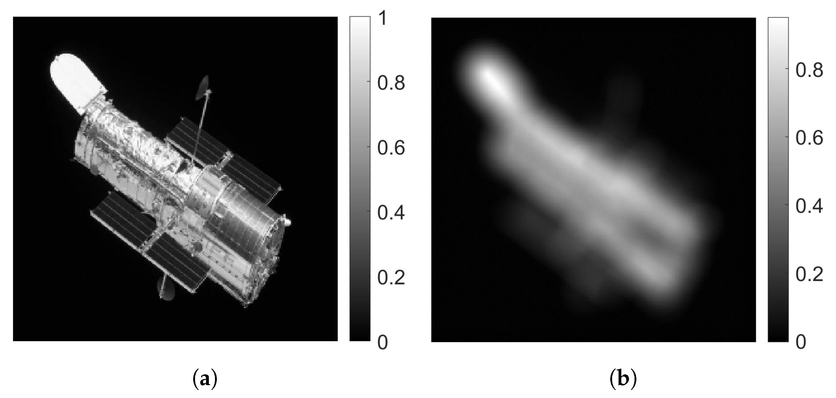
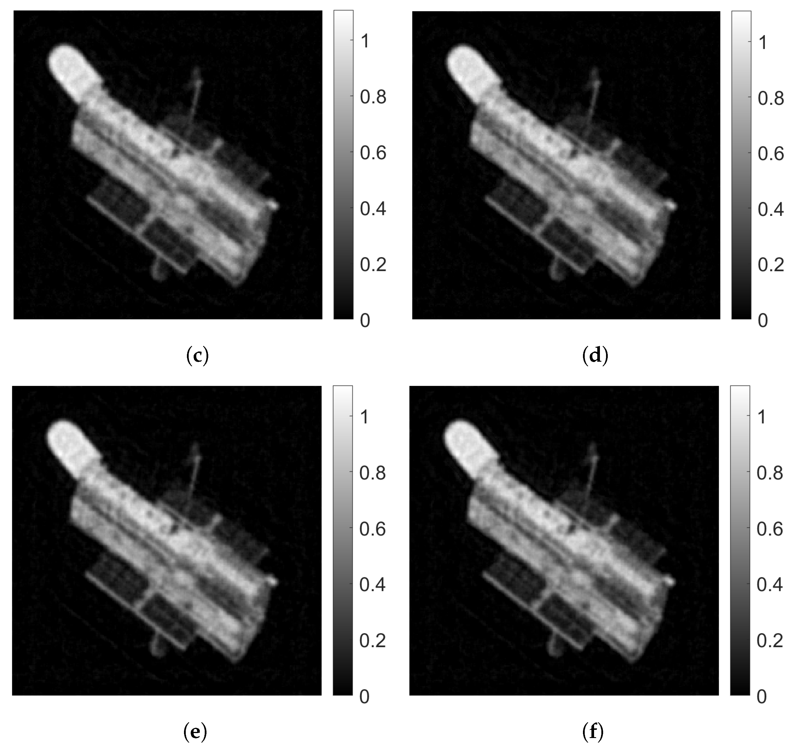
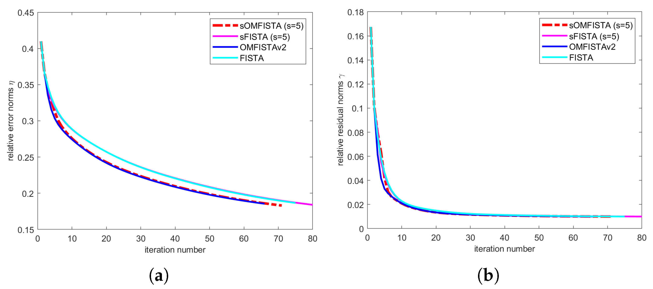
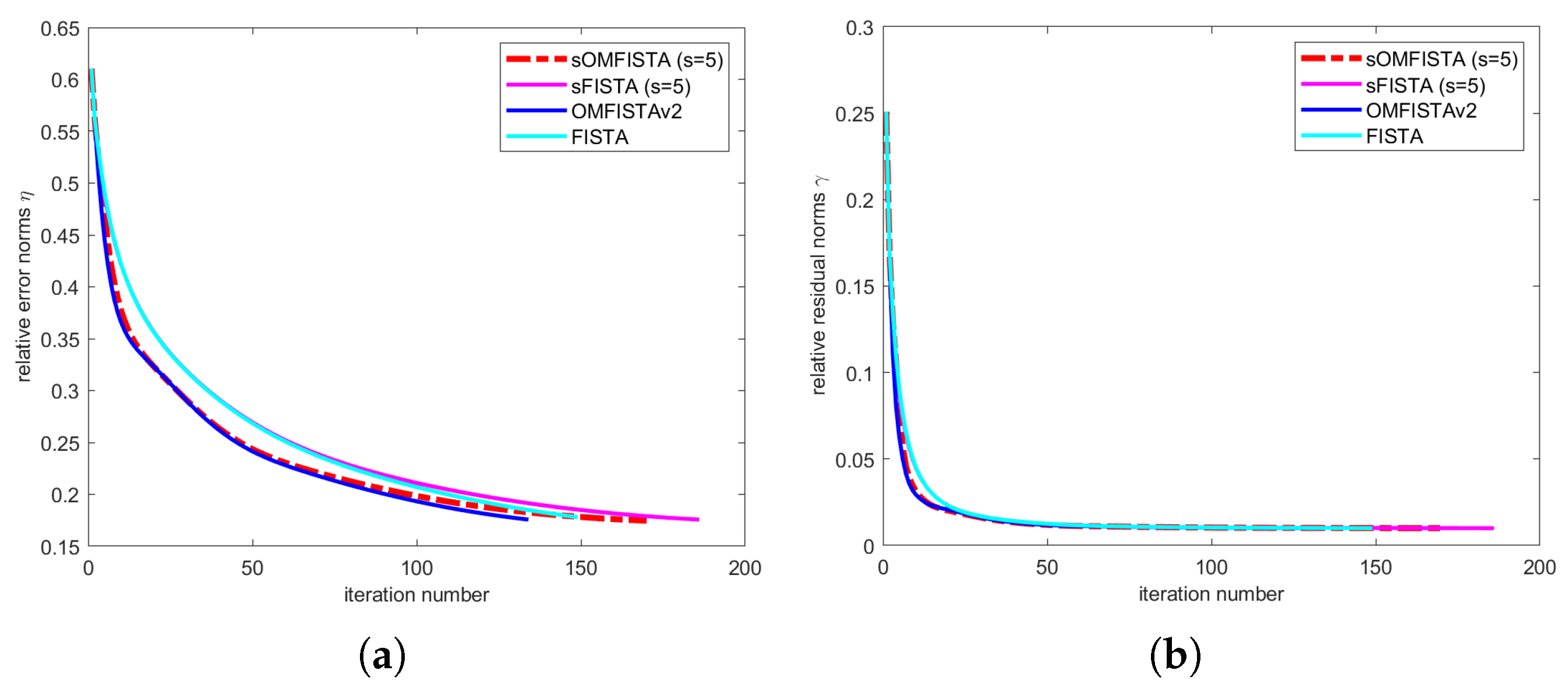
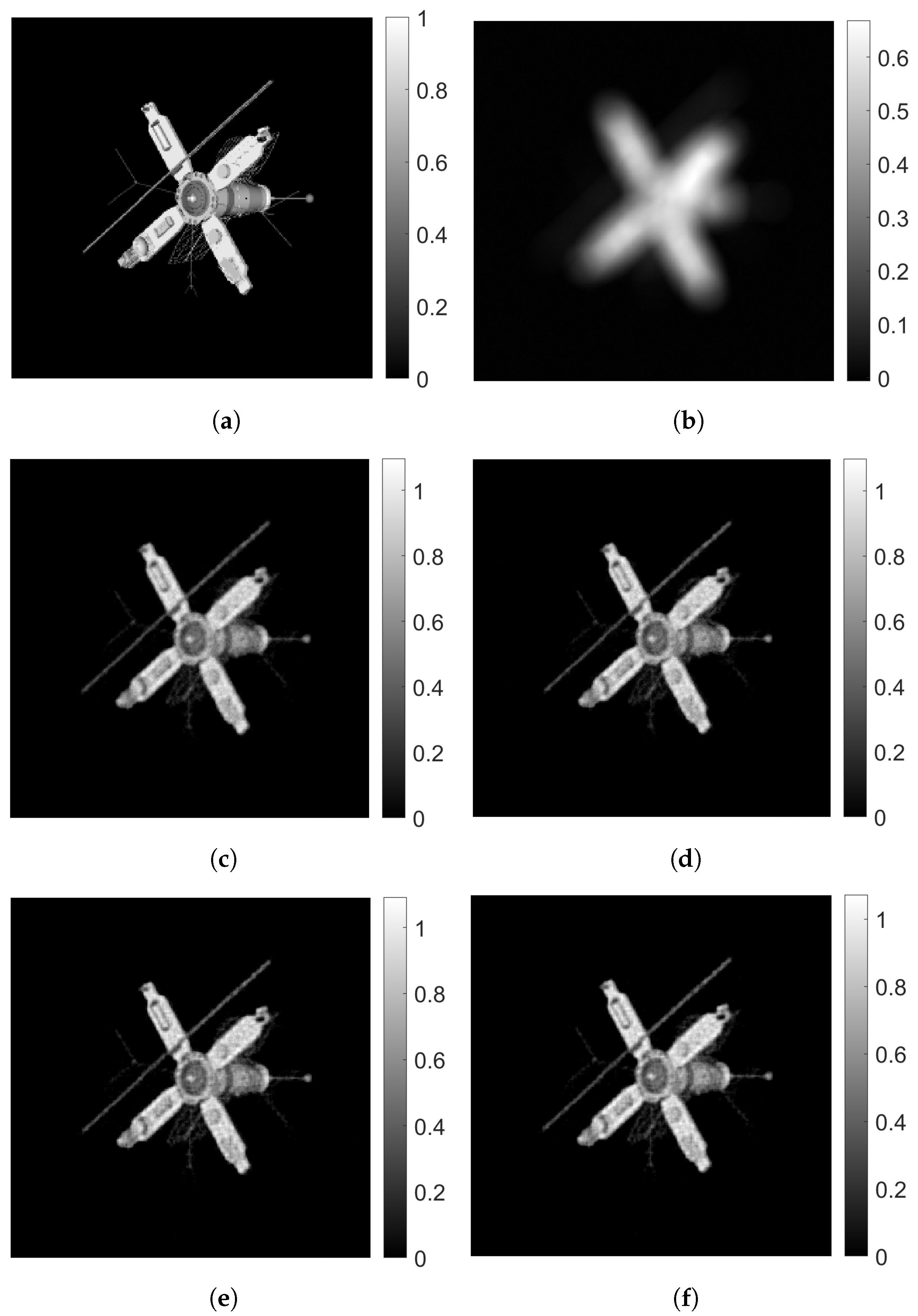
To show the performance of the proposed sOMFISTA, we compare it with FISTA, OMFISTAv2 and sFISTA on test images ‘hst’ (image of the Hubble space telescope) and ‘satellite’ (satellite test image). All algorithms are stopped when the relative residual satisfies $\gamma \le ϵ$ ($ϵ={10}^{-2}$) or the iteration number reaches 200. In sOMFISTA and sFISTA, s was set to be 5. In sOMFISTA and OMFISTAv2, $\alpha =0.5$, $\beta =1$, and $\theta =1$. Some numerical results, including the iteration number, the CPU time (seconds), the relative error η, the relative residual γ, the Mean Squared Error (MSE), the Peak Signal-to-Noise Ratio (PSNR) and the Structural Similarity Index (SSIM) are provided in

Table 3. Performance comparison of different algorithms on the test image ‘hst’.

	Iter	Time	$\mathit{\eta }$	$\mathit{\gamma }$	MSE	PSNR	SSIM
FISTA	74	$5.96$	$1.88\times {10}^{-1}$	$9.99\times {10}^{-3}$	330.0589	22.9449	0.8109
OMFISTAv2	66	$5.32$	$1.85\times {10}^{-1}$	$9.99\times {10}^{-3}$	329.4946	22.9523	0.8130
sFISTA	79	$1.74$	$1.85\times {10}^{-1}$	$9.99\times {10}^{-3}$	327.4294	22.9796	0.8098
sOMFISTA	71	$1.37$	$1.83\times {10}^{-1}$	$9.98\times {10}^{-3}$	325.2754	23.0083	0.8121

and

Table 4. Performance comparison of different algorithms on the test image ‘satellite’.

	Iter	Time	$\mathit{\eta }$	$\mathit{\gamma }$	MSE	PSNR	SSIM
FISTA	149	$12.00$	$1.78\times {10}^{-1}$	$9.99\times {10}^{-3}$	254.4559	24.0747	0.9510
OMFISTAv2	134	$10.88$	$1.76\times {10}^{-1}$	$9.99\times {10}^{-3}$	252.9799	24.0999	0.9503
sFISTA	186	$3.61$	$1.76\times {10}^{-1}$	$9.99\times {10}^{-3}$	249.5913	24.1585	0.9517
sOMFISTA	170	$2.92$	$1.75\times {10}^{-1}$	$9.99\times {10}^{-3}$	236.1671	24.3986	0.9527

. Figure 1 presents the visual results of ‘hst’ image restoration, comparing our proposed sOMFISTA method with other algorithms. To show how the relative error η and the relative residual γ evolve, we plot them versus the iteration number for all algorithms in Figure 2 and Figure 3. The visual results of ‘satellite’ image restoration are presented in Figure 4.

It is easy to see from the results in Table 3 and Table 4 that the proposed sOMFISTA method is faster and more accurate than the other three algorithms. sOMFISTA method consistently achieves the lowest MSE and highest PSNR, indicating the best reconstruction accuracy. Notably, it also delivers the fastest execution time among all algorithms, while maintaining competitive SSIM values and iteration counts. These results demonstrate that sOMFISTA effectively balances efficiency and precision, outperforming the other algorithms.

The top row of Figure 1 and Figure 4 shows the true image and the blurred and noisy image. The middle row of Figure 1 and Figure 4 shows reconstructed images using FISTA and OMFISTAv2. The bottom row of Figure 1 and Figure 4 shows reconstructed images using sFISTA and sOMFISTA. It is easy to see that the reconstructed image provided by sOMFISTA with $s=5$ is quite similar to that provided by FISTA.

Example 3.

To verify that the computational efficiency of sOMFISTA is robust for different blur levels, noise levels and images, four different test images extracted from the IR Tools toolbox are used in this example, which are represented by ‘satellite’ (satellite test image), ‘dot2’ (two small Gaussian shaped dots), ‘pattern1’ (geometrical image) and ‘ppower’ (random image with patterns of nonzero pixels), respectively. All the test images undergo a blurring procedure with three different blurring levels (‘mild’, ‘medium’, and ‘severe’), and are added Gaussian white with three different noise levels (${10}^{-3}$, ${10}^{-2}$, and ${10}^{-1}$). In sFISTA and sOMFISTA, s is set to be 5. In sOMFISTA and OMFISTAv2, $\alpha =0.5$, $\beta =1$, and $\theta =1$. The algorithm is stopped when the relative residual satisfies $\gamma \le ϵ$ ($ϵ={10}^{-2}$) or the iteration number reaches 200.

The computational time of the four algorithms on the four test images in this example extracted from functions PRblurdefocus are tabulated in

Table 5. Time of four algorithms for four test images under 3 noise and 3 blur levels.

Test Image	Noise Level	Blur Level	FISTA	OMFISTAv2	sFISTA	sOMFISTA
‘satellite’	${10}^{-3}$	Mild	$2.41$	$2.01$	$0.64$	$0.48$
		Medium	$3.24$	$2.88$	$0.83$	$0.72$
		Severe	$4.25$	$3.28$	$1.08$	$0.73$
	${10}^{-2}$	Mild	$6.30$	$5.82$	$1.50$	$1.36$
		Medium	$11.93$	$10.65$	$3.58$	$2.85$
		Severe	$15.72$	$15.60$	$3.87$	$3.19$
	${10}^{-1}$	Mild	$15.67$	$15.62$	$3.88$	$3.19$
		Medium	$15.72$	$16.23$	$3.87$	$3.31$
		Severe	$15.91$	$16.47$	$3.89$	$3.37$
‘dot2’	${10}^{-3}$	Mild	$5.08$	$3.88$	$1.19$	$0.84$
		Medium	$8.91$	$6.02$	$2.96$	$1.72$
		Severe	$15.54$	$15.61$	$3.93$	$3.06$
	${10}^{-2}$	Mild	$15.38$	$15.75$	$3.84$	$3.11$
		Medium	$15.16$	$15.29$	$3.85$	$3.10$
		Severe	$15.81$	$15.03$	$3.86$	$3.16$
	${10}^{-1}$	Mild	$15.66$	$15.53$	$3.79$	$3.13$
		Medium	$15.46$	$15.59$	$3.84$	$3.15$
		Severe	$15.26$	$15.74$	$3.83$	$3.13$
‘pattern1’	${10}^{-3}$	Mild	$1.17$	$0.93$	$0.33$	$0.25$
		Medium	$1.83$	$1.52$	$0.50$	$0.37$
		Severe	$2.38$	$2.04$	$0.59$	$0.45$
	${10}^{-2}$	Mild	$3.42$	$3.07$	$0.89$	$0.69$
		Medium	$5.76$	$5.44$	$1.58$	$1.22$
		Severe	$10.85$	$10.60$	$3.27$	$2.57$
	${10}^{-1}$	Mild	$15.69$	$15.53$	$3.86$	$3.19$
		Medium	$15.14$	$15.48$	$3.80$	$3.13$
		Severe	$15.48$	$15.81$	$3.95$	$3.26$
‘ppower’	${10}^{-3}$	Mild	$1.53$	$1.19$	$0.41$	$0.32$
		Medium	$15.61$	$15.46$	$3.81$	$3.19$
		Severe	$15.41$	$15.68$	$3.82$	$3.11$
	${10}^{-2}$	Mild	$3.17$	$2.83$	$0.86$	$0.64$
		Medium	$15.33$	$15.55$	$3.88$	$3.24$
		Severe	$15.82$	$15.59$	$3.80$	$3.16$
	${10}^{-1}$	Mild	$15.34$	$15.74$	$4.46$	$3.59$
		Medium	$15.71$	$15.59$	$3.81$	$3.19$
		Severe	$15.19$	$15.39$	$3.85$	$3.11$

. It is easy to see that sOMFISTA is faster than the other three algorithms for all test images with different blur and noise levels, which shows that the computational efficiency of sOMFISTA does not depend on the test images, the blurring type, the blurring or the noise levels.

5. Conclusions

In this paper, the sOMFISTA algorithm is proposed for solving large-scale ill-posed linear inverse problems arising from image restoration. The Kronecker product approximation of the blurring matrix and the over-relaxation technique are both exploited to accelerate the computation. The algorithm exhibits prominent advantages in computational efficiency and broad applicability to non-smooth convex regularization terms as verified by numerical experiments. sOMFISTA provides a reliable and efficient numerical tool for image restoration tasks, and its flexible framework paves the way for future applications in other ill-posed inverse problem scenarios.