Differential Topology and Matrix Analysis: An Overview

Abstract

This overview illustrates the application of methods from differential topology to several important problems in matrix analysis. In particular, it focuses on the use of smooth manifolds and smooth mappings to study fundamental issues such as the determination of matrix rank and the computation of the Jordan form in the presence of uncertainties. Various aspects of numerical matrix analysis are discussed, including the genericity of matrix problems, characterization of singular sets in the parameter space, the distance to ill-posedness and its relation to problem conditioning. The conditioning of matrix problems is considered in both deterministic and probabilistic settings. The paper also addresses the regularization of ill-posed matrix problems in the presence of errors. Several examples are provided to illustrate these concepts and their practical relevance. The overview is intended for specialists from different fields who use matrix analysis in their work and do not have a strong background in differential topology.

1. Introduction

Contemporary mathematical models used across the natural sciences are typically not single models corresponding to fixed parameter values; rather, they represent families of models that vary as parameters change within certain bounds. Such models arise in physics, chemistry, biology, control theory, statistics, aerodynamics, hydrodynamics, the social sciences, and several other disciplines. Studying such models using traditional methods is challenging, since the properties of a family cannot be described as continuous functions of the parameters when only individual fixed models are considered. This difficulty necessitates the use of families of models whose descriptions and properties depend smoothly on the parameters. Consequently, in recent years, specialists from various scientific fields have shown growing interest in methods of differential topology, whose objects of study are smooth manifolds and smooth mappings. Representing mathematical models in the natural sciences as smooth manifolds, with dimensions determined by the number of independent parameters, allows the essential properties of families of models to be expressed as smooth functions of these parameters, thereby greatly facilitating the solution of the corresponding mathematical problems. In this connection, it is appropriate to cite the German mathematician and philosopher Hermann Weyl, who wrote (p. 90, [1]): Topology has the peculiarity that questions belonging to its domain may under certain circumstances be decidable, even though the continua to which they are addressed may not be given exactly but only vaguely, as is always the case in reality.

Differential topology is a branch of mathematics that studies the global shape and structure of manifolds. A key idea is how local behavior influences the overall, global structure. Another important concept is transversality, which describes how two manifolds intersect. Understanding transversality helps explain which intersections are typical and stable under small changes.

The present overview aims to illustrate the application of methods from differential topology to the solution of some important mathematical problems arising across the natural and applied sciences. In particular, it focuses on the use of smooth manifolds and smooth mappings in matrix analysis, a field with wide-ranging applications in physics, engineering, biology, and beyond. The motivation for this overview stems from the absence of a single comprehensive reference on this subject.

This overview is intended for specialists in different fields who use matrix analysis in their work and do not have a strong background in differential topology. It can be useful for readers who are familiar, from a computational perspective, with issues such as sensitivity to perturbations, ill-conditioning, and numerical stability, but who have not previously encountered their geometric interpretation. At the same time, the paper may serve as a useful reference for readers with a background in differential topology who are interested in concrete applications to matrix problems. It should be noted that some mathematical rigor has been deliberately relaxed to make the exposition accessible to specialists from different disciplines.

The overview is organized into six sections.

In Section 2, we present the basic concepts from differential topology necessary for the subsequent discussion. We briefly consider smooth manifolds and smooth maps between them, including the differential of a map and singular points of varieties. Some fundamental facts about Lie groups and matrix groups are also included.

Section 3 is devoted to the geometry of matrix spaces. We examine important characteristics of problems in this space, such as genericity and well-posedness. Condition numbers of matrix problems are discussed in detail to demonstrate the connection between the distance to ill-posedness and problem conditioning. We also present results on the probabilistic distribution of matrix condition numbers obtained using methods from differential topology.

The important problem of matrix rank is considered in Section 4. We study the orbits of matrices with different ranks and show how small matrix perturbations can move a matrix to an orbit with lower codimension. The problem of determining the numerical rank of a matrix in the presence of uncertainties is also discussed.

Another fundamental problem in matrix analysis—the determination of the Jordan form of a matrix—is addressed in Section 5. We consider orbits and bundles of matrices with fixed Jordan form and investigate their generic properties. The reduction to the “true” Jordan form is described as an ill-posed problem, whose solution can be obtained via regularization methods. This leads to the concept of the numerical Jordan form, which is defined using the tools of differential topology.

In Section 6, we study matrices depending on parameters. It is shown that smooth structural properties of such matrices can be analyzed using versal deformations. Several examples of bifurcation diagrams are provided to illustrate how the Jordan form of a matrix depends on the varying parameters.

All computations in this paper were performed using MATLAB^®Version 9.9 (R2020b) [2], employing IEEE double precision arithmetic with a unit roundoff $\mathrm{u}\approx 1.11\times {10}^{-16}$.

2. A Glimpse into Differential Topology

Differential topology combines the study of the qualitative properties of manifolds of arbitrary dimension, which belongs to topology, with methods of classical analysis that enable quantitative investigation under small parametric variations. The questions addressed by differential topology are global in nature, as they concern the manifold as a whole.

The presentation in this section follows the classic textbooks by Guillemin and Pollack [3], Lee [4,5], Arnold [6,7], and Mishchenko and Fomenko [8], as well as the books by Tu [9] and by Burns and Gidea [10], which are written in a language accessible to non-mathematicians. Excellent introductions to manifold theory for non-specialists include the books by Milnor [11] and Wallace [12]. One of the most authoritative sources in this field is the book of Hirsch [13]; however, reading it requires a strong mathematical background. Applications of manifolds in mechanics are discussed in depth in [14]. Recent expositions on differential topology and its applications can be found in [15,16,17] as well as in the Special Issue of the journal Axioms devoted to Differential Geometry and Algebraic Topology [18]. The historical development of differential topology until 1960 is presented in detail in [19] and its subsequent progress up to 2010 is described in [20].

2.1. Smooth Manifolds

A manifold is a multidimensional generalization of the concepts of a line and a surface, without singular points. When studying manifolds, the notion of dimension plays a central role. Generally speaking, the dimension is the number of independent quantities (or parameters) required to specify a point on the manifold. Manifolds of dimension one are lines and curves, while manifolds of dimension two are surfaces. Typical examples of two-dimensional manifolds include planes and spheres, as well as other familiar surfaces such as cylinders, ellipsoids, paraboloids, and tori. A key feature of these examples is that an n-dimensional manifold “looks” locally like ${\mathbb{R}}^n$: every point of a manifold $\mathcal{M}$ has a neighborhood that is topologically equivalent to an open subset of ${\mathbb{R}}^n$. Thus, in one-dimensional manifolds each point has a neighborhood resembling a line segment; in two-dimensional manifolds, each point has a neighborhood resembling an open disk; and in three-dimensional manifolds, a neighborhood resembling an open ball.

In this sense, a manifold is a set in which the neighborhood of every point has the same local topological structure as n-dimensional Euclidean space.

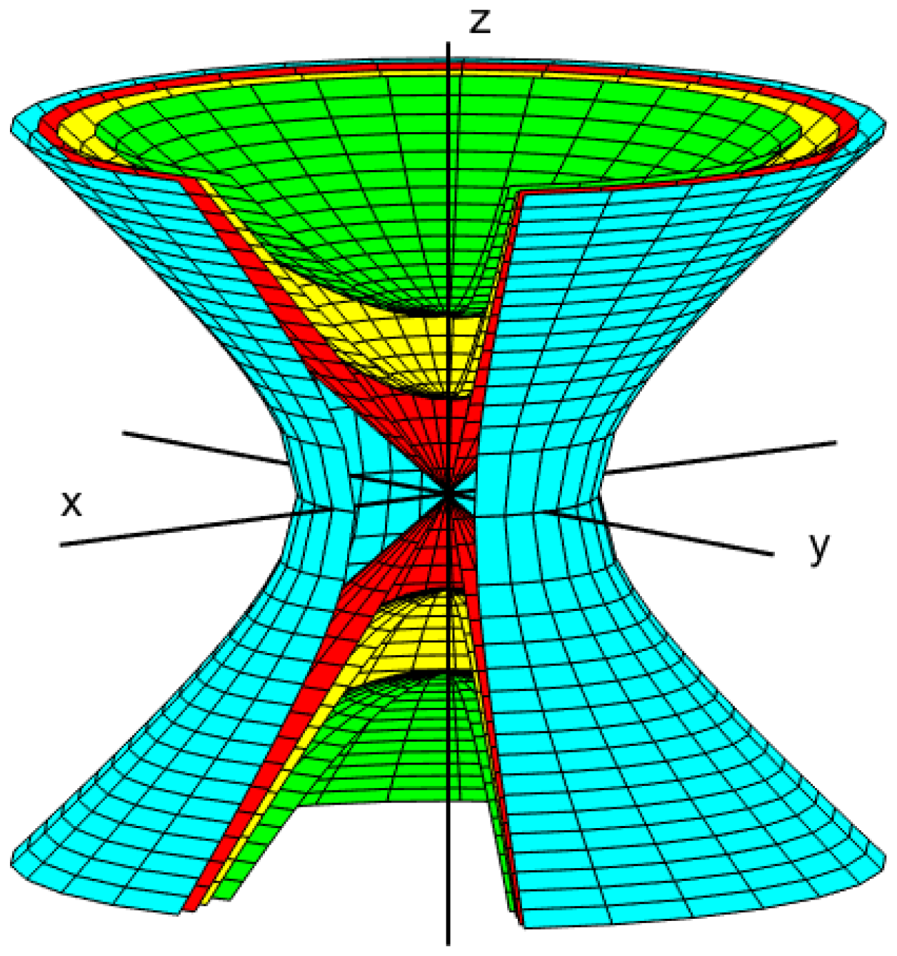
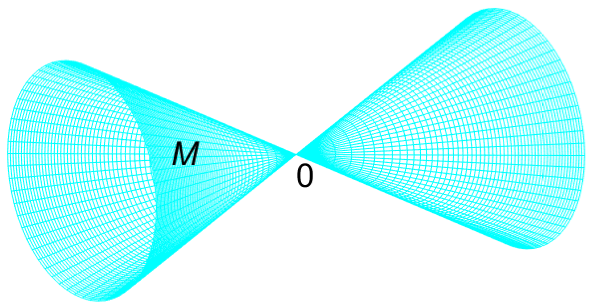
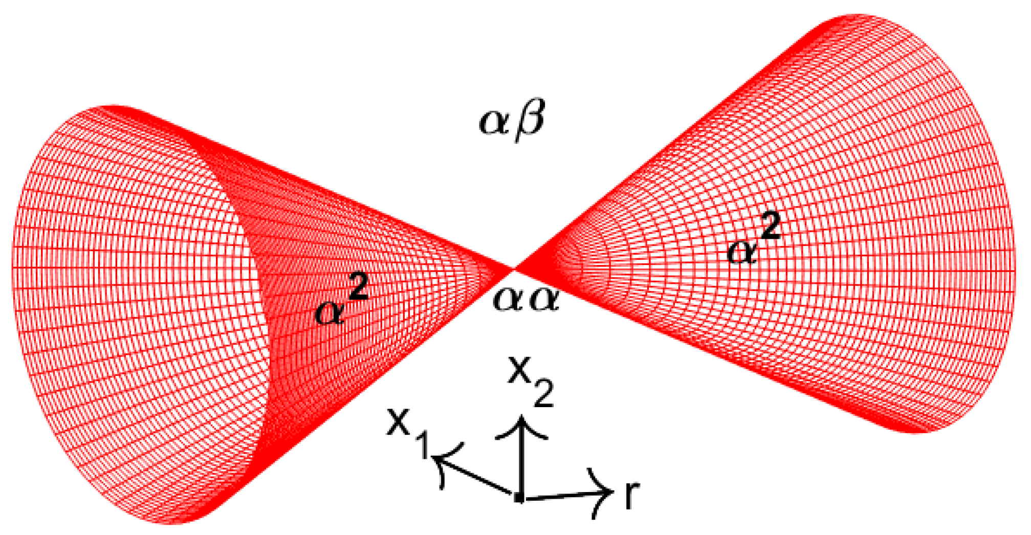
We note that the concept of dimension, as used in the characterization of manifolds, belongs to the most fundamental ideas in mathematics. An excellent overview of the significance of this concept in geometry and algebra is given by Manin in [21]. In Figure 1 we illustrate the decomposition of three-dimensional Euclidean space into layers (or strata) of manifolds defined by the equation $x^2+y^2-z^2=C$ for different values of C. An essential feature of this decomposition is that the individual layers do not intersect. Note that the innermost layer (the two opposite cones with a common vertex at the origin) is not smooth; rather, it is an algebraic variety, since the vertex is a singular point (see Section 2.7).

Definition 1.  

Two subsets of Euclidean spaces $U\subseteq {\mathbb{R}}^k,V\subseteq {\mathbb{R}}^n$ are topologically equivalent, or homeomorphic (from the Greek word meaning “similar form”), if there exists a one-to-one correspondence $\phi :U\to V$, such that both φ and its inverse are continuous. Such a correspondence is called a homeomorphism.

Based on these considerations, a provisional definition of a topological manifold can be given. We can consider an n-dimensional manifold as a subset of some Euclidean space ${\mathbb{R}}^k$ that is locally Euclidean of dimension n, i.e., every point of $\mathcal{M}$ has a neighborhood in $\mathcal{M}$ that is homeomorphic to a ball in ${\mathbb{R}}^n$.

For example, every one-dimensional manifold is homeomorphic to either a line or a circle.

In most cases, the analysis of manifolds cannot be performed directly on the manifold itself. Instead, it is necessary to describe the manifold unambiguously in an appropriate coordinate space and to apply analytical methods to this representation. For this purpose, coordinate charts and a manifold atlas are employed.

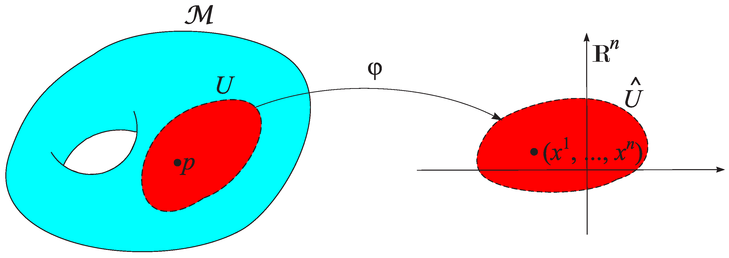
An open chart of $\mathcal{M}$ is defined as a pair $(U,\phi )$, where U is an open subset of the space $\mathcal{M}$, and $\phi$ is a homeomorphism from U onto an open subset of the coordinate space ${\mathbb{R}}^n$. To each point $p\in U$ there corresponds, in a one-to-one manner, an n-tuple of numbers

$$\phi :p\in U\mapsto (x^1\left(p\right),\dots ,x^n\left(p\right))\in \phi \left(U\right),$$

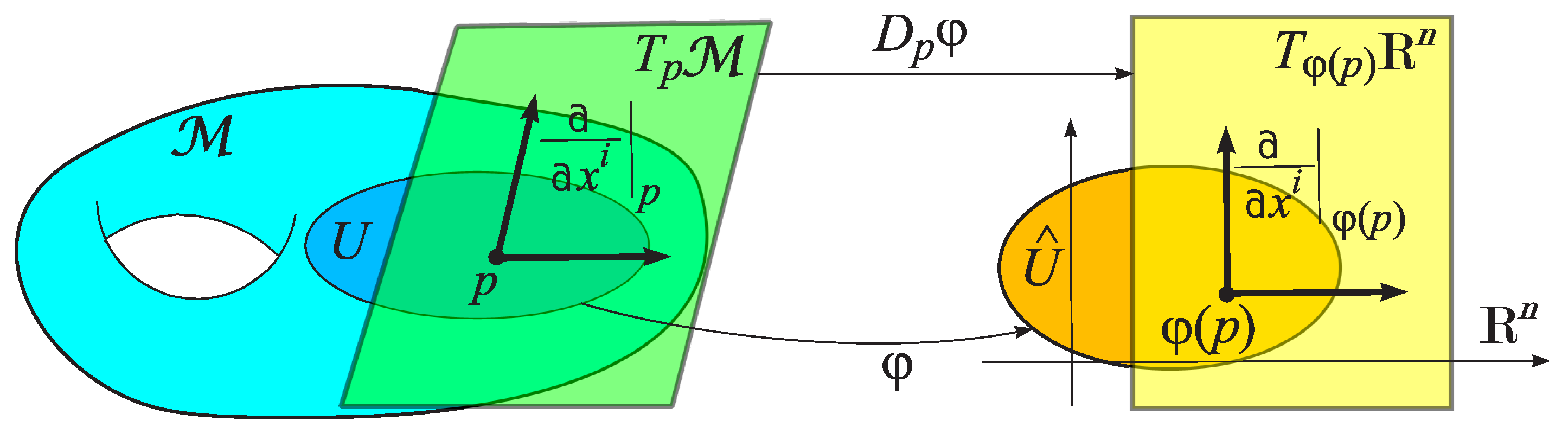
which are called its local coordinates (Figure 2). (Following the usual convention, we denote the indices of vectors by subscripts and their coordinates by superscripts.)

On the basis of the concept of an open chart, a rigorous definition of a topological manifold can be introduced.

Definition 2. 

Let A be a finite or countable set. A topological space $\mathcal{M}$ is called an n-dimensional topological manifold if there exists a collection of open charts $(U_{\alpha },{\phi }_{\alpha }),\alpha \in A$, such that:

• For each α of the set A, ${\phi }_{\alpha }\left(U_{\alpha }\right)$ is an open subset of ${\mathbb{R}}^n$.
• $\mathcal{M}={\bigcup }_{\alpha \in A}{U}_{\alpha }$.

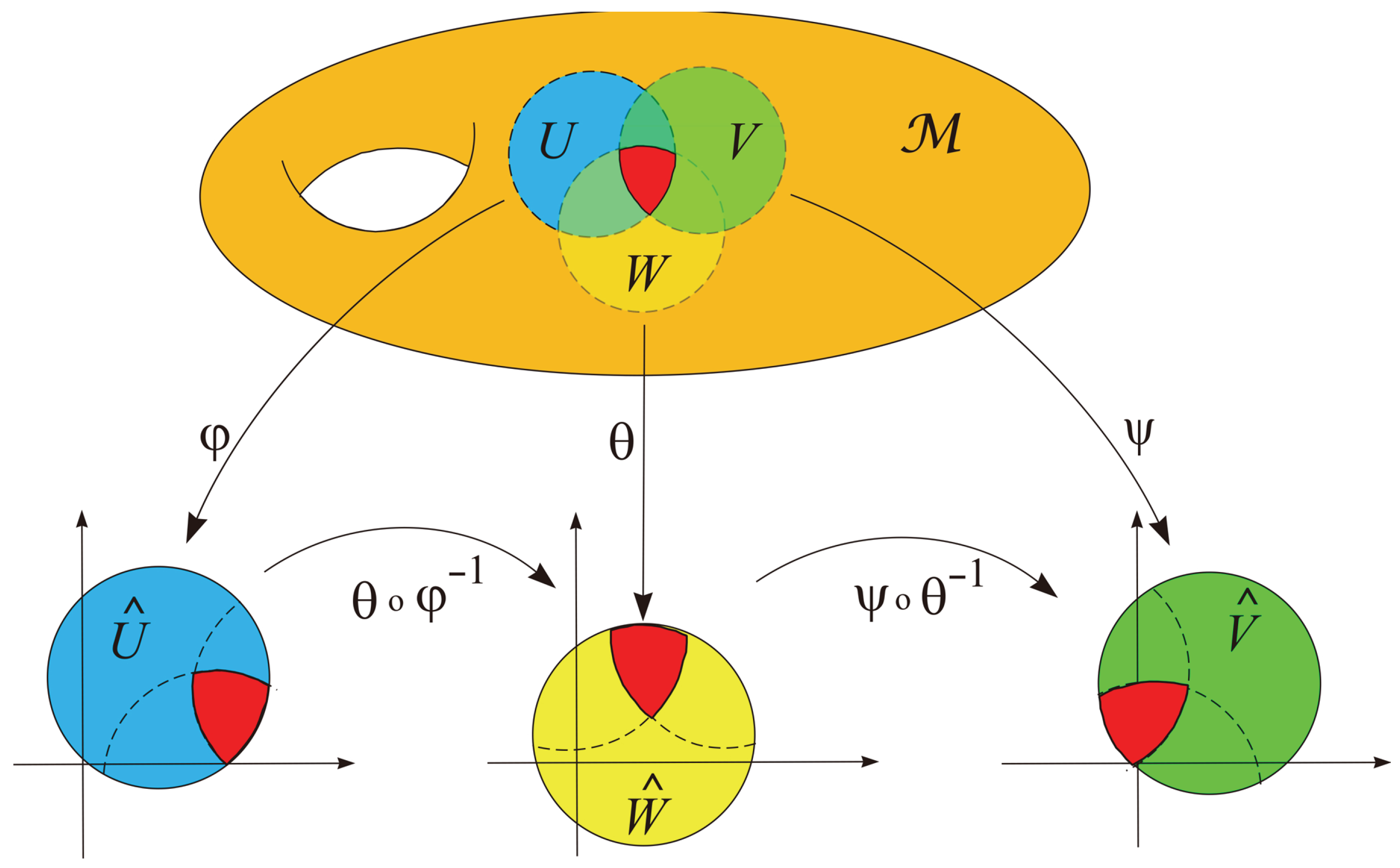
Such a collection of charts is called an atlas of the topological manifold (Figure 3). The atlas of $\mathcal{M}$ is denoted by $\mathcal{A}\left(\mathcal{M}\right)$.

In the general case, each chart $(U_i,{\phi }_i)$ is obtained using a different mapping ${\phi }_i$ associated with the subset $U_i$. In this way, one can study complex manifolds composed of several subsets with different properties. This constitutes an important advantage of manifolds over simpler topological objects which consist of a single set with fixed properties and are described by only one chart.

Example 1. 

(a)

The coordinate space ${\mathbb{R}}^n$ is an n-dimensional topological manifold: its atlas consists of a single open chart $({\mathbb{R}}^n,i_{{\mathbb{R}}^n})$, where $i_{{\mathbb{R}}^n}:{\mathbb{R}}^n\to {\mathbb{R}}^n$ is the identity map.

(b)

(Atlas of the two-dimensional sphere).

Let $N=(0,\dots ,0,1)\in {\mathbb{S}}^k\subseteq {\mathbb{R}}^{k+1}$ denote the north pole of the k-dimensional sphere, and let $S=(0,\dots ,0,-1)$ denote its south pole.

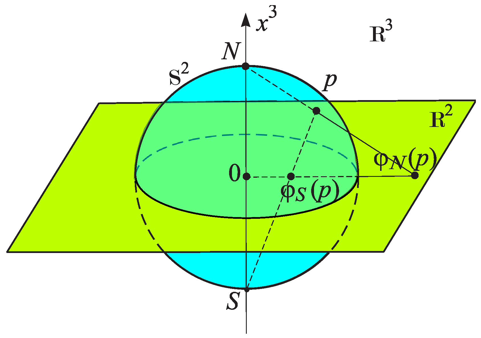
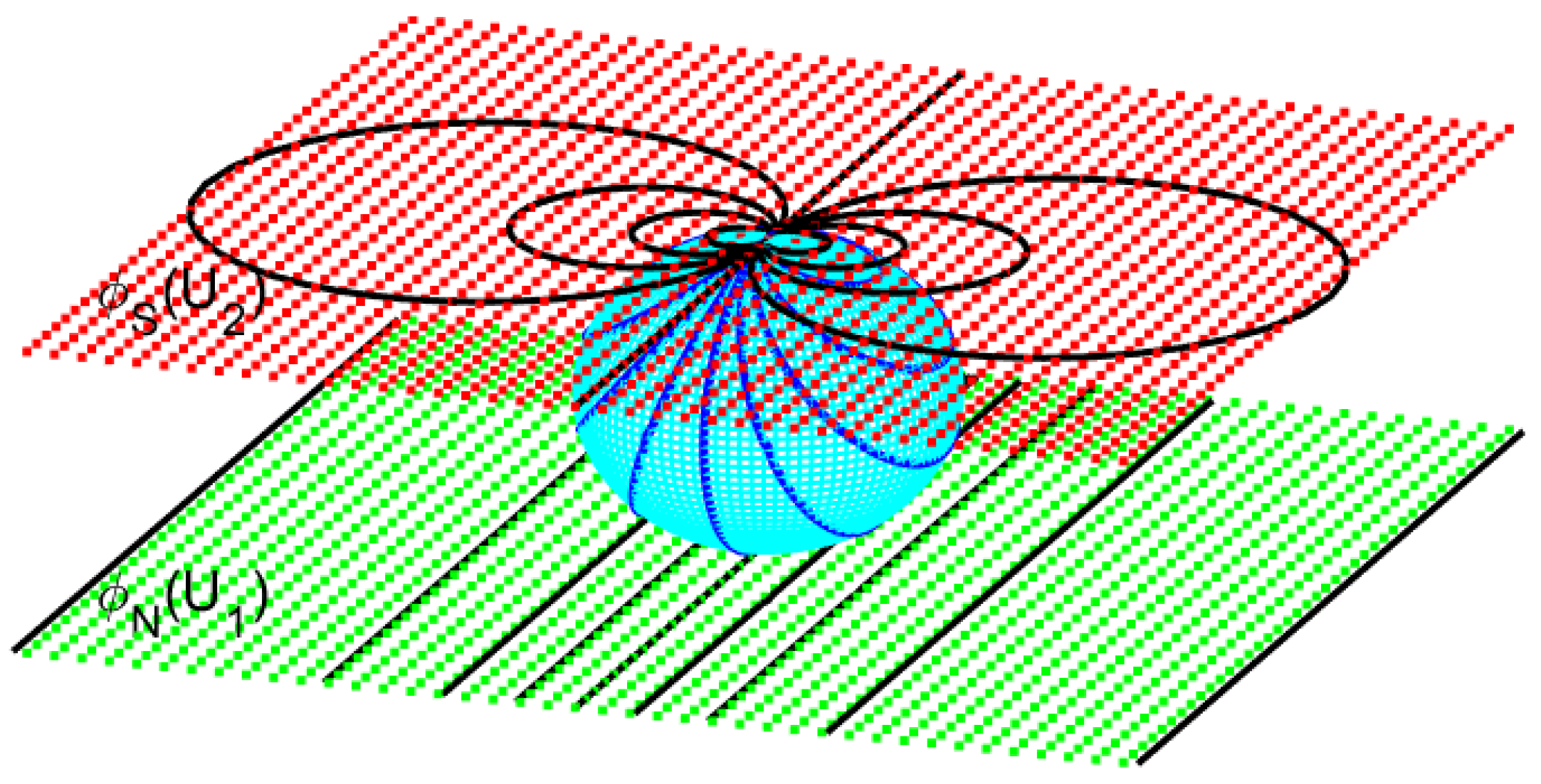
The stereographic projection ${\phi }_N$ from $U_1={\mathbb{S}}^k\setminus \left\{N\right\}$ onto ${\mathbb{R}}^k$ is the mapping that sends a point $p\in U_1$ to the intersection of the line through N and p with the linear subspace of ${\mathbb{R}}^{k+1}$ defined by $x^{k+1}=0$ (the projection plane). See Figure 4 for the case $k=2$. It defines a smooth bijective map from $U_1$ onto ${\mathbb{R}}^k$. Stereographic projection provides a way to represent the sphere by a plane and can also be applied to other curved surfaces, such as deformed spheres or hyperboloids.

The map

$${\phi }_N:{\mathbb{S}}^k\setminus \left\{N\right\}\to {\mathbb{R}}^k$$

is given explicitly by

$$(x^1,\dots ,x^{k+1})\mapsto {\displaystyle \frac{1}{1-x^{k+1}}}(x^1,\dots ,x^k).$$

Similarly, the projection ${\phi }_S$ from $U_2={\mathbb{S}}^k\setminus \left\{S\right\}$ onto ${\mathbb{R}}^k$ is given by

$$(x^1,\dots ,x^{k+1})\mapsto {\displaystyle \frac{1}{1+x^{k+1}}}(x^1,\dots ,x^k).$$

These projections are homeomorphisms from $U_1$ and $U_2$ onto ${\mathbb{R}}^k$. For ${\mathbb{S}}^2\subset {\mathbb{R}}^3$, we can define an atlas with two charts using stereographic projections:

$${\phi }_N\left(x\right)=\left({\displaystyle \frac{x^1}{1-x^3}},{\displaystyle \frac{x^2}{1-x^3}}\right),{\phi }_S\left(x\right)=\left({\displaystyle \frac{x^1}{1+x^3}},{\displaystyle \frac{x^2}{1+x^3}}\right),$$

where $U_1={\mathbb{S}}^2\setminus \left\{N\right\}$ and $U_2={\mathbb{S}}^2\setminus \left\{S\right\}$. These charts map the open sets $U_1$ and $U_2$ onto ${\mathbb{R}}^2$.

The atlas of the sphere is shown in Figure 5. The family of circles lying on the sphere and tangent at the point N is mapped in the lower chart to a family of parallel straight lines, while in the upper chart it is mapped to a family of tangent circles.

The definition of a topological space does not allow one to define differentiable functions or other concepts from mathematical analysis on a manifold. However, many important applications of manifolds involve mathematical analysis. For example, the application of manifold theory in geometry includes properties such as volume and curvature. Typically, volumes are computed by integration, while curvatures are determined through differentiation, so extending these concepts to manifolds requires a way to make integration and differentiation meaningful on a manifold.

Similarly, applications in classical mechanics involve solving ordinary differential equations on manifolds. To give these concepts meaning, it is necessary to define an additional structure on the manifold. In order to make sense of derivatives of real-valued functions, curves, or manifolds, it is necessary to introduce a new type of manifold called a smooth manifold. This is a topological manifold equipped with an additional structure compatible with its topology, which allows one to determine which functions to or from the manifold are smooth.

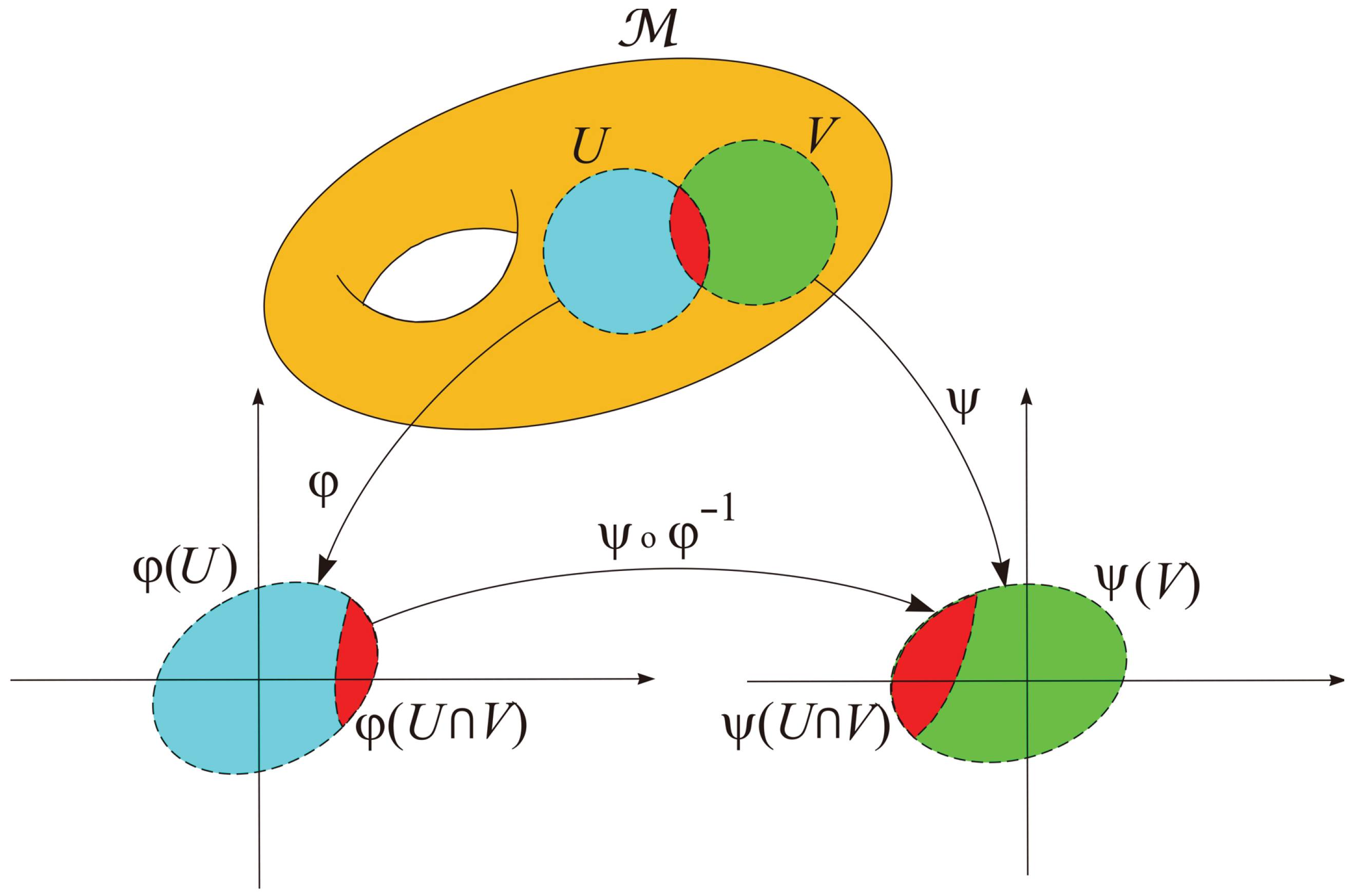
Let $\mathcal{M}$ be an n-dimensional topological manifold, and let $\mathcal{A}$ be an atlas of the manifold $\mathcal{M}$. Consider any two charts in the atlas $\mathcal{A}$, denoted by $(U,\phi )$ and $(V,\psi )$ (Figure 6).

Definition 3. 

The coordinate transformation

$$\psi \circ {\phi }^{-1}:\phi (U\cap V)\subset {\mathbb{R}}^n\to \psi (U\cap V)\subset {\mathbb{R}}^n,$$

which maps the intersection $\phi (U\cap V)$ in ${\mathbb{R}}^n$ to $\psi (U\cap V)$ in ${\mathbb{R}}^n$, is called smooth if the transition functions

$$\begin{array}{ccc}\hfill y^1& =\hfill & \hfill y^1(x^1,\dots ,x^n),\\ \hfill ⋮& \hfill & \hfill ⋮\\ \hfill y^n& =\hfill & \hfill y^n(x^1,\dots ,x^n)\end{array}$$

have continuous partial derivatives of all orders (that is, they are infinitely differentiable, belonging to the class $C^{\infty }$ in the open set $\phi (U\cap V)$), and the determinant

$$\det \left(\left[{\displaystyle \frac{\partial y^i}{\partial x^j}}\right]\right),$$

of the Jacobian matrix of the transformation is nonzero.

This also implies that the inverse coordinate transformation of ${(\psi \circ {\phi }^{-1})}^{-1}=\phi \circ {\psi }^{-1}$ is smooth, since the corresponding transition functions

$$\begin{array}{ccc}\hfill x^1& =\hfill & \hfill x^1(y^1,\dots ,y^n),\\ \hfill ⋮& \hfill & \hfill ⋮\\ \hfill x^n& =\hfill & \hfill x^n(y^1,\dots ,y^n)\end{array}$$

have continuous partial derivatives of all orders in the open set $\psi (U\cap V)$.

If the coordinate transformation is smooth, we say that the corresponding charts are smoothly compatible.

An atlas $\mathcal{A}$ is called smooth if:

• Any two charts in the atlas are smoothly compatible.
• Every point $p\in \mathcal{M}$ lies in the domain of at least one chart.

A smooth atlas $\mathcal{A}$ on $\mathcal{M}$ is called maximal if it is not properly contained in any larger smooth atlas. This means that any chart that is smoothly compatible with every chart in $\mathcal{A}$ is already included in $\mathcal{A}$. A maximal atlas is also called a complete atlas.

Definition 4. 

An n-dimensional topological manifold $\mathcal{M}$ is said to have a smooth structure if there exists an atlas $\mathcal{A}$ on the manifold satisfying the following properties:

• For any two charts in $\mathcal{A}$, the corresponding coordinate transformation is smooth.
• The atlas $\mathcal{A}$ is maximal.

Definition 5. 

An n-dimensional topological manifold that has a smooth structure is called an n-dimensional smooth manifold.

Example 2. 

(a)

(Normed vector spaces). Let V be a finite-dimensional real vector space. Any norm on V defines a topology that is independent of the choice of norm. With this topology, V is an n-dimensional topological manifold with a natural smooth structure defined as follows. Any (ordered) basis $(e_1,\dots ,e_n)$ of V defines a basic isomorphism $E:{\mathbb{R}}^n\to V$ by

$$E\left(x\right)=\sum _{i=1}^n{x}^i{e}_i.$$

This map is a homeomorphism, so $(V,E^{-1})$ is a chart. The collection of all such charts defines a smooth structure, called the standard smooth structure on V.

(b)

(Matrix spaces). Let $\mathcal{M}(m\times n,\mathbb{R})$ denote the set of $m\times n$ matrices with real entries. Since it is a real vector space of dimension $m·n$ under matrix addition and scalar multiplication, $\mathcal{M}(m\times n,\mathbb{R})$ is a smooth $m·n$-dimensional manifold. (Since the spaces $\mathcal{M}(m\times n,\mathbb{R})$ and ${\mathbb{R}}^{m·n}$ are isometric, they can be identified by “stacking” all matrix entries into a single row or column.) A chart on this manifold is given by

$$\phi :{\mathbb{R}}^{m\times n}\to {\mathbb{R}}^{m·n}:X\mapsto \mathrm{vec}\left(X\right),$$

where $\mathrm{vec}\left(X\right)$ denotes the vector obtained from the matrix entries as described above. The dimension of this manifold is $m·n$. The space ${\mathbb{R}}^{m\times n}$ can be equipped with a Euclidean structure via the inner product

$$\langle M_1,M_2\rangle =\mathrm{vec}{\left(M_1\right)}^T\mathrm{vec}\left(M_2\right)=\mathrm{tr}\left(M_1^T{M}_2\right).$$

The norm induced by this inner product is the Frobenius norm, defined by

$${\parallel M\parallel }_F^2=\mathrm{tr}\left(M^{T}M\right),$$

i.e., ${\parallel M\parallel }_F^2$ is the sum of the squares of all entries of M.

Similarly, the space $\mathcal{M}(m\times n,\mathbb{C})$ of $m\times n$ complex matrices is a vector space of dimension $2mn$ over $\mathbb{R}$ and therefore is a smooth manifold of dimension $2·m·n$. In the special case $m=n$ (square matrices), the notations $\mathcal{M}(m\times n,\mathbb{R})$ and $\mathcal{M}(m\times n,\mathbb{C})$ are abbreviated as $\mathcal{M}(n,\mathbb{R})$ and $\mathcal{M}(n,\mathbb{C})$, respectively.

(c)

(General linear group). The general linear group $\mathrm{GL}(n,\mathbb{R})$ is the set of invertible $n\times n$ matrices with real entries. It is an $n^2$-dimensional manifold because it is an open subset of the $n^2$-dimensional vector space $\mathcal{M}(n,\mathbb{R})$, namely the set where the (continuous) determinant function $det\left(A\right)$ is nonzero.

(d)

(Spaces of linear maps). Let V and W be finite-dimensional real vector spaces, and let $L(V,W)$ denote the set of linear maps from V to W. Since $L(V,W)$ is itself a finite-dimensional vector space (whose dimension is the product of the dimensions of V and W), it naturally carries the structure of a smooth manifold, just as in item (b).

A submanifold of a manifold $\mathcal{M}$ is a subset $\mathcal{P}\subset \mathcal{M}$ that itself has the structure of a manifold. The sphere ${\mathbb{S}}^2$, defined by the equation $x^2+y^2+z^2=1$, is an example of a subset of the coordinate space ${\mathbb{R}}^3$ that inherits its manifold structure from ${\mathbb{R}}^3$.

In a number of important applications of manifolds, one encounters spaces that would be smooth manifolds except that they have a “boundary” of some kind. Elementary examples of such spaces are closed intervals in $\mathbb{R}$, closed balls in ${\mathbb{R}}^n$, and closed hemispheres in ${\mathbb{S}}^n$. The study of manifolds with boundary requires a generalization of the definition of a manifold; see, for example, (Ch. 1, [5]).

An overview of the historical development of the concept of a manifold can be found in [22].

2.2. Smooth Maps

Let $U\subset {\mathbb{R}}^n$ be an open set. Any mapping $f:U\to {\mathbb{R}}^m$ can be represented as an ordered collection of m functions:

$$f(x^1,\dots ,x^n)=\left(f^1(x^1,\dots ,x^n),f^2(x^1,\dots ,x^n),\dots ,f^m(x^1,\dots ,x^n)\right).$$

The mapping $f:U\to {\mathbb{R}}^m$ is called smooth ($f\in C^{\infty }$), if each function $f^k,k=1,2,\dots ,m$, has continuous partial derivatives of all orders. A mapping whose components are continuous is called a $C^0$ mapping. In the case where all functions $f^k$ are analytic (a function is called analytic if its Taylor series converges to it in a neighborhood of each point), the mapping f is called analytic ($f\in C^{\omega }$). We have the inclusion $C^{\infty }\supset C^{\omega }$.

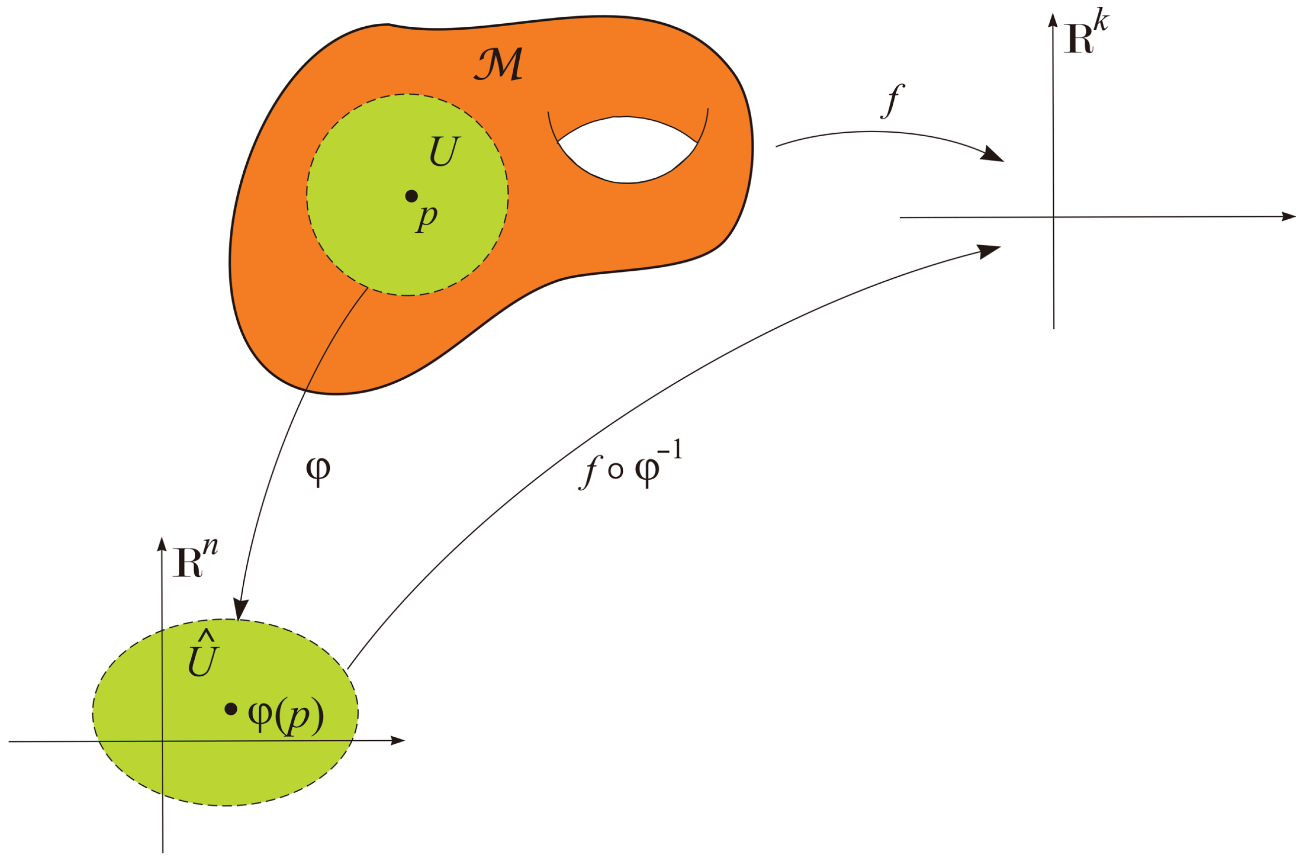
Let us consider first the case of a vector-valued function defined on a manifold. Suppose that $\mathcal{M}$ is an n-dimensional manifold, k is a nonnegative integer, and $f:\mathcal{M}\to {\mathbb{R}}^k$ is an arbitrary function. 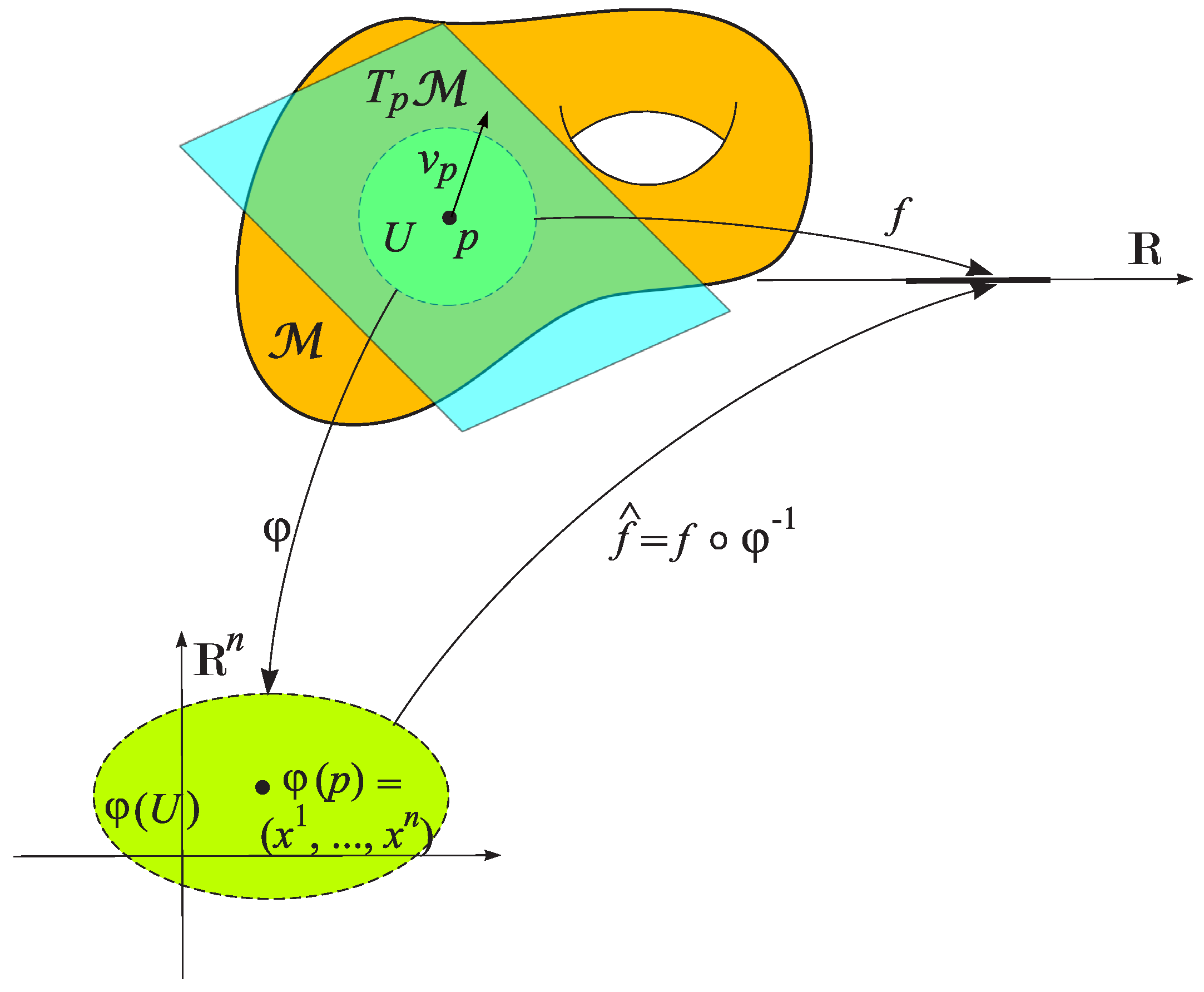We say that f is a smooth function if, for every point $p\in \mathcal{M}$, there exists a smooth chart $(U,\phi )$ of $\mathcal{M}$ whose domain U contains p and such that the composite function $f\circ {\phi }^{-1}$ is smooth on the open subset $\widehat{U}=\phi \left(U\right)\subseteq {\mathbb{R}}^n$ (see Figure 7).

For a given function $f:\mathcal{M}\to {\mathbb{R}}^k$ and a chart $(U,\phi )$ of $\mathcal{M}$, the function $\widehat{f}:\phi \left(U\right)\to {\mathbb{R}}^k$, defined by $\widehat{f}=f\circ {\phi }^{-1}$, is called coordinate representation of f. By definition, f is smooth if and only if its coordinate representation is smooth in some smooth chart around every point.

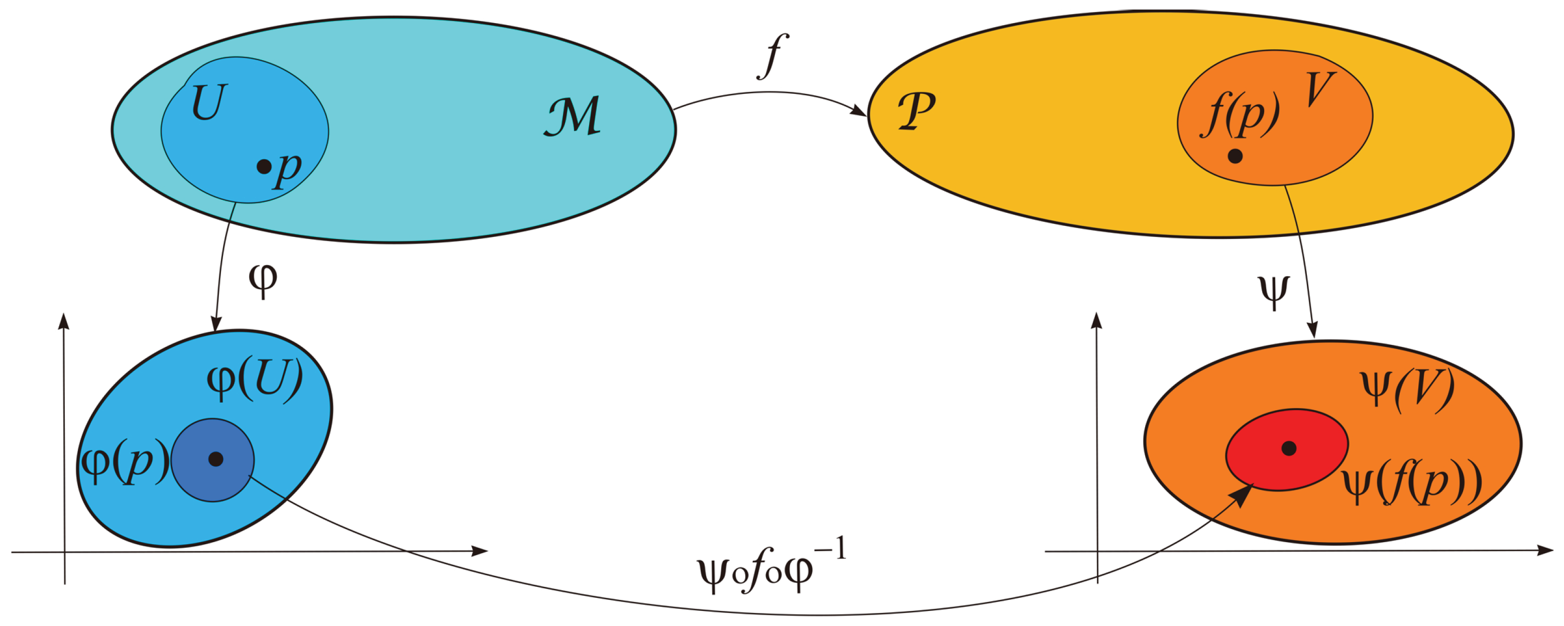
Let $\mathcal{M}$ and $\mathcal{P}$ be smooth manifolds of dimensions n and k, respectively, and let $f:\mathcal{M}\to \mathcal{P}$ be an arbitrary map. The map f is called smooth at the point p of the manifold $\mathcal{M}$ if there exist a local chart $(U,\phi )$ containing p and a local chart $(V,\psi )$ containing $f\left(p\right)$ such that $f\left(U\right)\subseteq V$ and the composition

$$\psi \circ f\circ {\phi }^{-1}$$

is a smooth map from $\phi \left(U\right)$ to $\psi \left(V\right)$ (Figure 8).

A map f is called smooth if it is smooth at every point p of the manifold $\mathcal{M}$ (see Figure 9).

Every smooth map is continuous.

The set of smooth maps of the form $f:\mathcal{M}\to \mathcal{P}$ is denoted by $C^{\infty }(\mathcal{M},\mathcal{P})$.

Let $\mathcal{M}$ and $\mathcal{P}$ be smooth manifolds.

A smooth map $f:\mathcal{M}\to \mathcal{P}$ is called a diffeomorphism if it is bijective and its inverse $f^{-1}:\mathcal{P}\to \mathcal{M}$ is also smooth.

The manifold $\mathcal{M}$ is said to be diffeomorphic to the manifold $\mathcal{P}$ if there exists a diffeomorphism $f:\mathcal{M}\to \mathcal{P}$. This is denoted by $\mathcal{M}\cong \mathcal{P}$.

Example 3. 

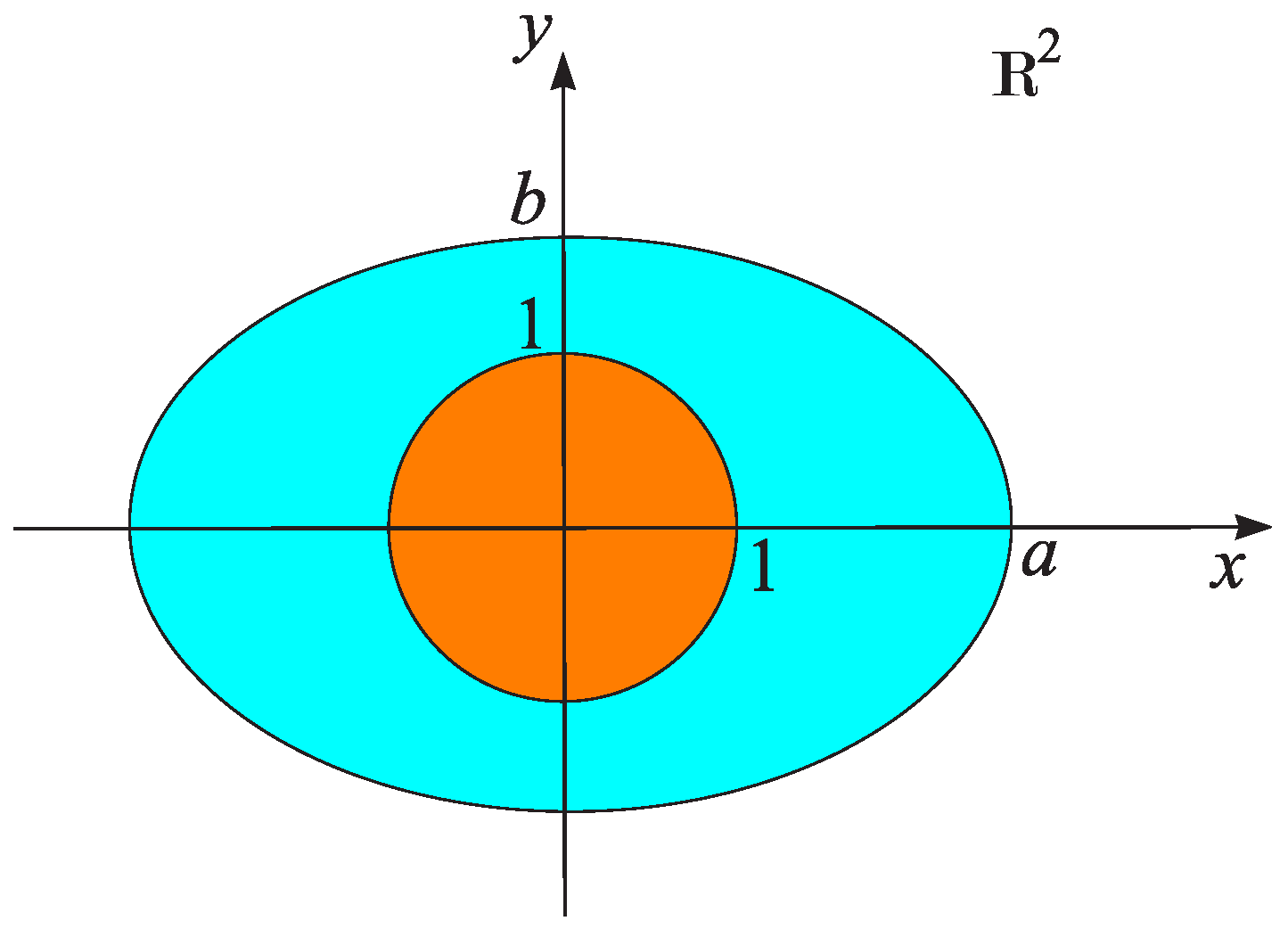
In Figure 10, an open disk and an open ellipse are shown, which are diffeomorphic. The disk is mapped to the ellipse by the smooth map

$$f:(x,y)\mapsto (ax,by),$$

and the ellipse is mapped back to the disk by the inverse map

$$f^{-1}:(x,y)\mapsto (x/a,y/b),$$

which is also smooth.

Figure 10. The ellipse ${\displaystyle \frac{x^2}{a^2}}+{\displaystyle \frac{y^2}{b^2}}<1$ and the open disk $x^2+y^2<1$ are diffeomorphic.

Figure 10. The ellipse ${\displaystyle \frac{x^2}{a^2}}+{\displaystyle \frac{y^2}{b^2}}<1$ and the open disk $x^2+y^2<1$ are diffeomorphic.

Similar to the case when two topological spaces are considered “the same” if they are homeomorphic, two smooth manifolds are regarded as indistinguishable if they are diffeomorphic. A central question in the theory of smooth manifolds is the study of properties of smooth manifolds that are preserved under diffeomorphisms.

2.3. Tangent Space

In the study of the metric properties of regions in Euclidean space, an important role is played by properties that are defined in a theoretically infinitesimal neighborhood of a fixed point, by neglecting quantities of higher order relative to the distance to that point. Similarly, in the study of smooth manifolds it is appropriate to neglect infinitesimal quantities of higher order in order to simplify the analysis of a given problem. One way to achieve this is to introduce special concepts analogous to tangent vectors to curves and tangent planes to surfaces, as used in mathematical analysis.

Let $v_p$ be a vector in the coordinate space ${\mathbb{R}}^n$ based at a point $p\in {\mathbb{R}}^n$. Then, for every smooth function f defined in a neighborhood of the point p, the directional derivative determined by the vector $v_p$ is defined as follows:

$${\left.{\displaystyle \frac{\partial f}{\partial v}}\right|}_p=\underset{t\to 0}{lim}{\displaystyle \frac{f(p+t{v}_p)-f\left(p\right)}{t}}={\displaystyle \frac{d}{dt}}f(p+t{v}_p){|}_{t=0},$$

where t is a numerical parameter (in analysis, one usually considers a vector $v_p$ of unit length). In a coordinate system, we have the formula:

$${\left.{\displaystyle \frac{\partial f}{\partial v}}\right|}_p={\left.{\displaystyle \frac{\partial f}{\partial x^1}}\right|}_p{v}^1+\dots +{\left.{\displaystyle \frac{\partial f}{\partial x^n}}\right|}_p{v}^n={\langle \mathrm{grad}\left(f\left(p\right)\right),v\rangle }_p,$$

where

$$\mathrm{grad}\left(f\right)=\left({\displaystyle \frac{\partial f}{\partial x^1}},\dots ,{\displaystyle \frac{\partial f}{\partial x^n}}\right)$$

is the gradient of the function f, and $x^1,\dots ,x^n$, $v^1,\dots ,v^n$ are the coordinates of the point p and the vector $v_p$, respectively. Furthermore, the quantity

$${\left.{\displaystyle \frac{\partial f}{\partial v}}\right|}_p=\sum _{i=1}^n{v}^i{\displaystyle \frac{\partial }{\partial x^i}}f\left(p\right)$$

will be called the derivative of the smooth function f in the direction of the vector $v_p$ at the point p and will be denoted by $D_p^{v}f$. In this notation, it is understood that the partial derivatives are evaluated at p, since $v_p$ is a vector at p. Note that $D_p^{v}f$ is a number, not a function. We write

$$D_p^v=\sum _{i=1}^n{v}^i{\left.{\displaystyle \frac{\partial }{\partial x^i}}\right|}_p$$

for the map that sends the function f to the number $D_p^{v}f$.

Thus, each vector $v_p$ at the point p defines determines a linear operator on the set of smooth functions defined in a neighborhood of p:

$$D_p^v:C^{\infty }\left(p\right)\to \mathbb{R},$$

performed according to the rule

$$f\left(p\right)\mapsto D_p^{v}f.$$

Definition 6. 

A tangent vector at point p of the manifold $\mathcal{M}$ is a rule

$$v_p:C^{\infty }\left(p\right)\to \mathbb{R},$$

which assigns to each function f in the set $C^{\infty }\left(p\right)$ a number $v_{p}f$ satisfying the following properties:

• $v_p(f+g)=v_{p}f+v_{p}g$,
• $v_p\left(\alpha f\right)=\alpha v_{p}f$,
• $v_p(f·g)=f\left(p\right)·v_{p}g+v_{p}f·g\left(p\right)$,

where $f,g\in C^{\infty }\left(p\right),\alpha \in \mathbb{R}$.

The association $v_p\mapsto D_p^v$ of the directional derivative $D_p^v$ with the tangent vector $v_p$ allows tangent vectors to be characterized as certain operators acting on functions.

The set of vectors that are tangent to the manifold $\mathcal{M}$ at a point p is denoted by $T_p\mathcal{M}$. We now define on this set the operations of addition of tangent vectors and scalar multiplication of a tangent vector.

Let $v_p,w_p\in T_p\mathcal{M},f\in C^{\infty }\left(p\right)$ and $\alpha \in \mathbb{R}$. We define

$$\begin{array}{ccc}\hfill (v_p+w_p)f& =\hfill & \hfill v_{p}f+w_{p}f,\\ \hfill \left(\alpha v_p\right)f& =\hfill & \hfill \alpha v_{p}f.\end{array}$$

It is not difficult to verify that both the sum of the tangent vectors $v_p$ and $w_p$ as well as the scalar product of a tangent vector with a scalar $\alpha v_p$ are also tangent vectors. In this way, the set $T_p\mathcal{M}$ becomes a vector space. It is called the tangent space to the smooth manifold $\mathcal{M}$ at the point p.

Let $(U,\phi )$ be a local chart (coordinate system) and let $p\in U$. For every function $f\in C^{\infty }\left(p\right)$ one can construct a smooth function $\widehat{f}=f\circ {\phi }^{-1}$, defined on the open subset $\phi \left(U\right)$ of ${\mathbb{R}}^n$ (see Figure 11).

By computing the partial derivatives of $\widehat{f}$ with respect to the variables $x^1,\dots ,x^n$, we obtain

$${\displaystyle \frac{\partial }{\partial x^i}}\widehat{f}\left(\phi \left(p\right)\right)={\left.{\displaystyle \frac{\partial }{\partial x^i}}\right|}_{\phi \left(p\right)}(f\circ {\phi }^{-1}),i=1,\dots ,n.$$

In this way, for each function $f\in C^{\infty }\left(p\right)$, one can associate n numbers

$$f\mapsto {\left.{\displaystyle \frac{\partial }{\partial x^1}}\right|}_{\phi \left(p\right)}(f\circ {\phi }^{-1}),\dots ,{\left.{\displaystyle \frac{\partial }{\partial x^n}}\right|}_{\phi \left(p\right)}(f\circ {\phi }^{-1}).$$

We see that the choice of a system of local coordinates determines n vectors in the tangent space $T_p\mathcal{M}$ acting according to the rule

$$f\mapsto {\left.{\displaystyle \frac{\partial }{\partial x^i}}\right|}_{\phi \left(p\right)}(f\circ {\phi }^{-1}),i=1,\dots ,n.$$

These vectors are conventionally denoted by

$${\left.{\displaystyle \frac{\partial }{\partial x^i}}\right|}_p.$$

The quantities $\partial /\partial x^i{|}_p$ represent linear partial differential operators, which act according to the rule

$${\left.{\displaystyle \frac{\partial }{\partial x^i}}\right|}_{p}f={\left.{\displaystyle \frac{\partial f}{\partial x^i}}\right|}_p={\left.{\displaystyle \frac{\partial }{\partial x^i}}\right|}_{\phi \left(p\right)}(f\circ {\phi }^{-1})={\displaystyle \frac{\partial \widehat{f}}{\partial x^i}}\left(\phi \left(p\right)\right).$$

Theorem 1 

([5], Ch. 3). The vectors

$${\left.{\displaystyle \frac{\partial }{\partial x^1}}\right|}_p,\dots ,{\left.{\displaystyle \frac{\partial }{\partial x^n}}\right|}_p$$

form a basis of the tangent space $T_p\mathcal{M}$.

In this way, we obtain the important result that the dimension of the tangent space $T_p\mathcal{M}$ is equal to the dimension of the manifold $\mathcal{M}$,

$$\dim \left(T_p\mathcal{M}\right)=\dim \left(\mathcal{M}\right).$$

Suppose $\mathcal{M}$ is an n-dimensional manifold embedded in ${\mathbb{R}}^k$. For each $p\in \mathcal{M}$ we define the normal space to $\mathcal{M}$ to be the $(k-n)$-dimensional subspace $N_p\mathcal{M}$ consisting of all vectors that are orthogonal to $T_p\mathcal{M}$ with respect to the Euclidean dot product.

Instead of working with the dimension of the manifold $\mathcal{M}$, it is often more convenient to use the codimension of $\mathcal{M}$, denoted by $\mathrm{codim}\left(\mathcal{M}\right)$, which is equal to the dimension of the normal space $N_p\mathcal{M}$. Since

$$T_p\mathcal{M}\oplus N_p\mathcal{M}={\mathbb{R}}^k,$$

we have

$$\dim \left(\mathcal{M}\right)+\mathrm{codim}\left(\mathcal{M}\right)=k.$$

2.4. Differential of a Map

To analyze the action of smooth maps on tangent vectors, it is necessary to consider the differentiation of such maps. In the case of a smooth map between Euclidean spaces, the total derivative of the map at a point (represented by its Jacobian matrix) is a linear map that provides the “best linear approximation” of the map near the given point. In the case of manifolds, a linear map is defined between the tangent spaces.

Definition 7. 

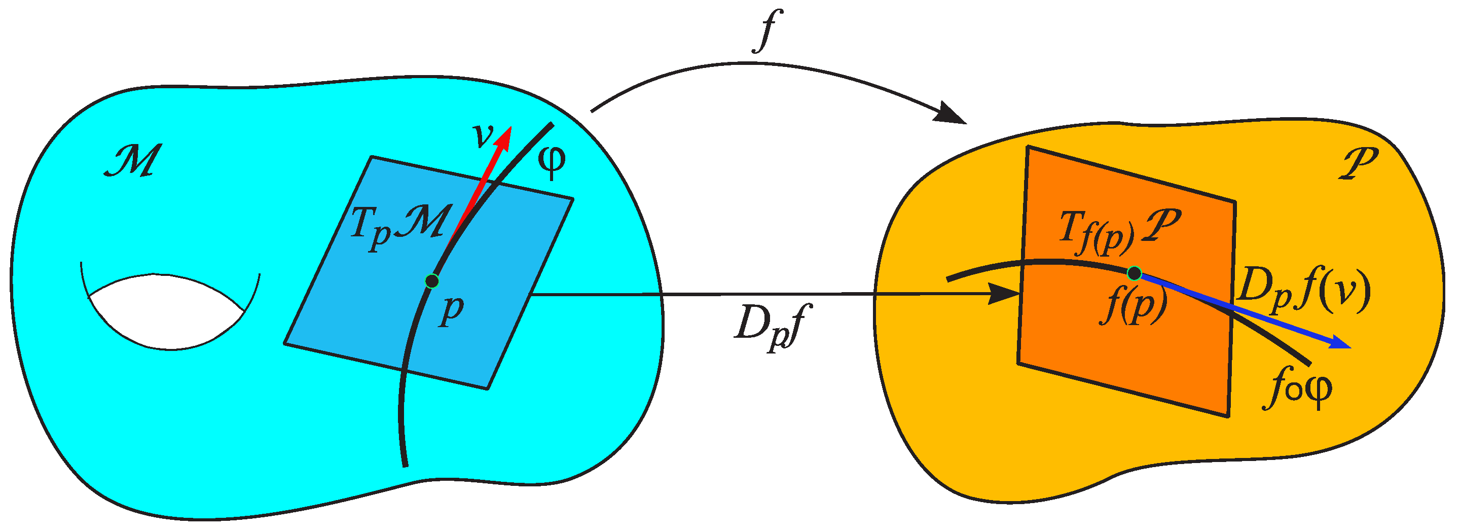
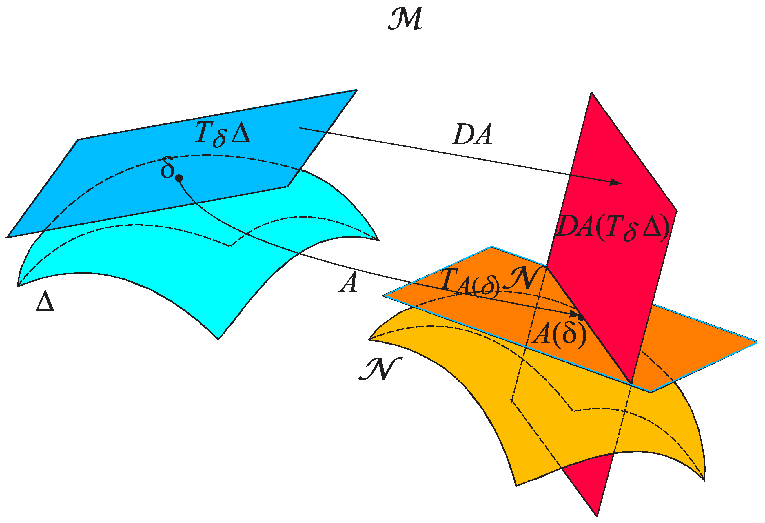
Let $\mathcal{M}$ and $\mathcal{P}$ be smooth manifolds, and let $f:\mathcal{M}\to \mathcal{P}$ be a smooth map. The differential of f at a point $p\in \mathcal{M}$ is the linear map

$$D_{p}f:T_p\mathcal{M}\to T_{f\left(p\right)}\mathcal{P},$$

defined as follows (see Figure 12). Let $v\in T_p\mathcal{M}$. Consider a smooth curve $\phi :\mathbb{R}\to \mathcal{M}$ with $\phi \left(0\right)=p$ whose tangent vector at 0 is v. Then $D_{p}f\left(v\right)$ is the tangent vector at 0 to the curve $f\circ \phi :\mathbb{R}\to \mathcal{P}$.

Proposition 1 

(Properties of the differential). Let $\mathcal{M}$, $\mathcal{P}$, and $\mathcal{Z}$ be smooth manifolds. Let $f:\mathcal{M}\to \mathcal{P}$ and $g:\mathcal{P}\to \mathcal{Z}$ be smooth maps, and let $p\in \mathcal{M}$.

(a)

$D_{p}f:T_p\mathcal{M}\to T_{f\left(p\right)}\mathcal{P}$ is a linear map.

(b)

$D_p(g\circ f)=D_{f\left(p\right)}g\circ D_{p}f:T_p\mathcal{M}\to T_{g\circ f\left(p\right)}\mathcal{Z}$.

(c)

$D_p\left(i_{\mathcal{M}}\right)=i_{T_p\mathcal{M}}:T_p\mathcal{M}\to T_p\mathcal{M}$, where $i_{\mathcal{M}}$ is the identity map on $\mathcal{M}$.

(d)

If f is a diffeomorphism, then $D_{p}f:T_p\mathcal{M}\to T_{f\left(p\right)}\mathcal{P}$ is an isomorphism, and ${\left(D_{p}f\right)}^{-1}=D_{f\left(p\right)}\left(f^{-1}\right)$.

Suppose that $\mathcal{M}$ is a smooth manifold without boundary, and let $(U,\phi )$ be a smooth coordinate chart on $\mathcal{M}$. Then, in particular, $\phi$ is a diffeomorphism from U onto an open subset $\widehat{U}\subseteq {\mathbb{R}}^n$. It can be shown that

$$D_p\phi :T_p\mathcal{M}\to T_{\phi \left(p\right)}{\mathbb{R}}^n$$

is an isomorphism. The coordinate basis vectors

$${\left.{\displaystyle \frac{\partial }{\partial x^1}}\right|}_{\phi \left(p\right)},\dots ,{\left.{\displaystyle \frac{\partial }{\partial x^n}}\right|}_{\phi \left(p\right)}$$

form a basis of $T_{\phi \left(p\right)}{\mathbb{R}}^n$, and the preimages of these vectors,

$${\left.{\displaystyle \frac{\partial }{\partial x^1}}\right|}_p,\dots ,{\left.{\displaystyle \frac{\partial }{\partial x^n}}\right|}_p,$$

under the isomorphism $D_p\phi$, form a basis of $T_p\mathcal{M}$ (Figure 13).

Using $(y^1,\dots ,y^m)$ to denote coordinates in the codomain of f, the action of $D_{p}f$ on a typical basis vector is

$$D_{p}f\left({\left.{\displaystyle \frac{\partial }{\partial x^i}}\right|}_p\right)=\sum _{j=1}^m{\displaystyle \frac{\partial f^j}{\partial x^i}}\left(p\right){\left.{\displaystyle \frac{\partial }{\partial y^j}}\right|}_{f\left(p\right)}.$$

(1)

Therefore, the matrix of $D_{p}f$ in terms of the coordinate bases is

$$\left[\begin{array}{ccc}{\displaystyle \frac{\partial f^1}{\partial x^1}}\left(p\right)& \dots & {\displaystyle \frac{\partial f^1}{\partial x^n}}\left(p\right)\\ ⋮& \ddots & ⋮\\ {\displaystyle \frac{\partial f^m}{\partial x^1}}\left(p\right)& \dots & {\displaystyle \frac{\partial f^m}{\partial x^n}}\left(p\right)\end{array}\right].$$

This matrix is precisely the Jacobian matrix of f at p, which is the matrix representation of the total derivative $Df\left(p\right):{\mathbb{R}}^n\to {\mathbb{R}}^m$.

Example 4. 

We consider the maps $f:{(-r,r)}^3\to {\mathbb{R}}^3$ and $g:{\mathbb{R}}^3\to {(-r,r)}_r^3$, defined by

$$\begin{array}{ccc}\hfill f\left(x\right)& =\hfill & \hfill \left({\displaystyle \frac{x^1}{\sqrt{1-{x^1}^2}}},{\displaystyle \frac{x^2}{\sqrt{1-{x^2}^2}}},{\displaystyle \frac{x^3}{\sqrt{1-{x^3}^2}}}\right),\\ \hfill g\left(x\right)& =\hfill & \hfill \left({\displaystyle \frac{x^1}{\sqrt{1+{x^1}^2}}},{\displaystyle \frac{x^2}{\sqrt{1+{x^2}^2}}},{\displaystyle \frac{x^3}{\sqrt{1+{x^3}^2}}}\right),\end{array}$$

where ${(-r,r)}^3\subset {\mathbb{R}}^3$ is the open cube with $0<r<1$.

These maps are smooth, and it can be shown that they are inverses of each other for all x such that $|x^i|<1$ for each coordinate i. Therefore, both maps are diffeomorphisms.

Let $p=(p^1,p^2,p^3)$ be a point on the sphere ${\mathbb{S}}_R^2$ that does not coincide with the north pole. To obtain the tangent space $T_{f\left(p\right)}f\left({\mathbb{S}}_R^2\right)$, we need to compute the differential $D_{p}f:{\mathbb{R}}^2\to T_{f\left(p\right)}f\left({\mathbb{S}}_R^2\right)$. For a local parametrization of ${\mathbb{S}}_R^2$ and $f\left({\mathbb{S}}_R^2\right)$ in ${\mathbb{R}}^2$, we use the stereographic projections (see Example 1)

$$\begin{array}{ccc}\hfill \phi :{\mathbb{S}}_R^2\to {\mathbb{R}}^2,(x^1,x^2)& =& \phi \left(p\right)=\left({\displaystyle \frac{p^1}{1-p^3}},{\displaystyle \frac{p^2}{1-p^3}}\right),\hfill \\ \hfill {\phi }^{-1}:{\mathbb{R}}^2\to {\mathbb{S}}_R^2,(p^1,p^2,p^3)& =& {\phi }^{-1}\left(x\right)={\displaystyle \frac{1}{1+{x^1}^2+{x^2}^2}}\left(2x^1,2x^2,{x^1}^2+{x^2}^2-1\right),\hfill \\ \hfill \psi :f\left({\mathbb{S}}_R^2\right)\to {\mathbb{R}}^2,\psi \left(y\right)& =& \left({\displaystyle \frac{y^1}{1-y^3}},{\displaystyle \frac{y^2}{1-y^3}}\right),\hfill \end{array}$$

where

$$y=f\left(p\right)=\left({\displaystyle \frac{p^1}{\sqrt{1-{p^1}^2}}},{\displaystyle \frac{p^2}{\sqrt{1-{p^2}^2}}},{\displaystyle \frac{p^3}{\sqrt{1-{p^3}^2}}}\right).$$

The matrices of partial derivatives are

$$\begin{array}{ccc}\hfill D_y\psi & =& \left[\begin{array}{ccc}1/(1-y^3)& 0& y^1/{(1-y^3)}^2\\ 0& 1/(1-y^3)& y^2/{(1-y^3)}^2\end{array}\right],\hfill \\ \hfill D_{p}f& =& \left[\begin{array}{ccc}1/{(1-{p^1}^2)}^{3/2}& 0& 0\\ 0& 1/{(1-{p^2}^2)}^{3/2}& 0\\ 0& 0& 1/{(1-{p^3}^2)}^{3/2}\end{array}\right],\hfill \\ \hfill D_x{\phi }^{-1}& =& {\displaystyle \frac{2}{{(1+{x^1}^2+{x^2}^2)}^2}}\left[\begin{array}{cc}1-{x^1}^2+{x^2}^2& -2x^1{x}^2\\ -2x^1{x}^2& 1+{x^1}^2-{x^2}^2\\ 2x^1& 2x^2\end{array}\right].\hfill \end{array}$$

The tangent space $T_{f\left(p\right)}f\left({\mathbb{S}}_R^2\right)$ is obtained as the image of ${\mathbb{R}}^2$ under the differential $D_{x}f=D_{p}f{D}_x{\phi }^{-1}$.

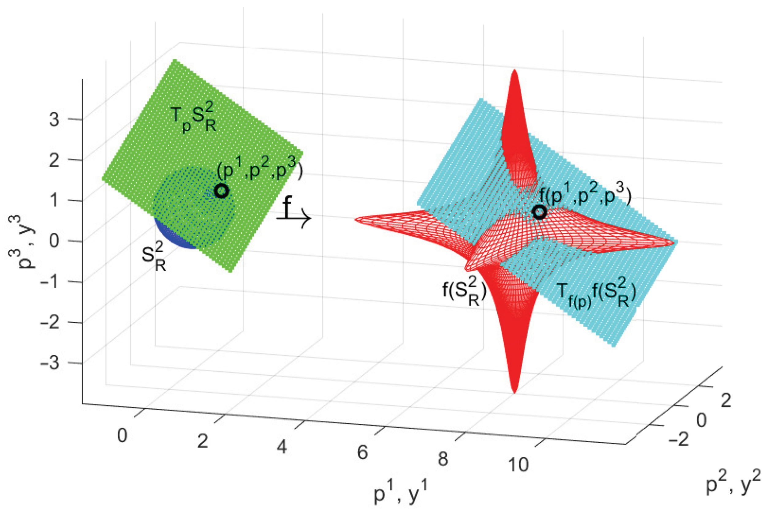
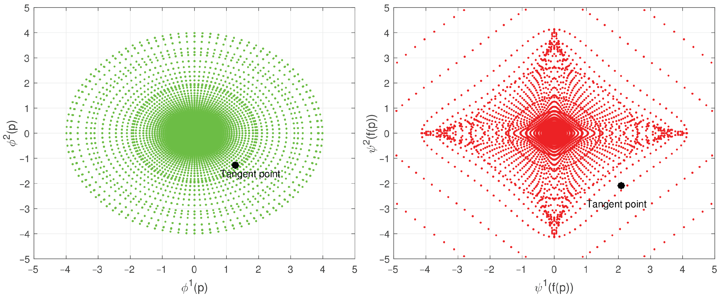
Figure 14 shows the diffeomorphic image ${\mathbb{S}}_R^2\mapsto f\left({\mathbb{S}}_R^2\right)$ of a sphere with radius $R=0.97$. The tangent spaces $T_p{\mathbb{S}}_R^2$ and $T_{f\left(p\right)}f\left({\mathbb{S}}_R^2\right)$ are computed for the points $p=R(1/\sqrt{3},-1/\sqrt{3},1/\sqrt{3})$ and $x=\phi \left(p\right),y=f\left(p\right)$.

In Figure 15, for the same mapping, the corresponding parts of the stereographic projection of the sphere and the stereographic projection of its diffeomorphic image onto ${\mathbb{R}}^2$ are shown, respectively.

The matrix of the differential $D_{\widehat{p}}\widehat{f}:{\mathbb{R}}^2\to {\mathbb{R}}^2$ is obtained from

$$D_{\widehat{p}}\widehat{f}=D_y\psi D_{p}f{D}_x{\phi }^{-1}.$$

Clear descriptions of tangent vectors and tangent spaces of manifolds, accompanied by examples, are given in (Ch. 3, [5]), (Ch. 3, [9]), (Ch. 1, [10]), (Ch. 4, [12]), [23], (Ch. 4, [24]).

2.5. Tangent and Normal Bundle

Let $\mathcal{M}$ be a smooth manifold. Let us define the disjoint union of all tangent spaces of $\mathcal{M}$,

$$T\mathcal{M}=\underset{p\in \mathcal{M}}{⨆}{T}_p\mathcal{M}.$$

The set $T\mathcal{M}$ is called the tangent bundle of the manifold $\mathcal{M}$. The term bundle indicates that $T\mathcal{M}$ consists of “layers” – the tangent spaces at the individual points of the manifold. The tangent bundle of an m-dimensional manifold is itself a manifold whose dimension is equal to $2m$.

In the trivial case, when $\mathcal{M}={\mathbb{R}}^n$, for each $p\in {\mathbb{R}}^n$ the tangent space $T_p{\mathbb{R}}^n$ can be identified with ${\mathbb{R}}^n$. Therefore, in this case we have $T{\mathbb{R}}^n\cong {\mathbb{R}}^n\times {\mathbb{R}}^n$, i.e., the tangent bundle $T{\mathbb{R}}^n$ is diffeomorphic to the Cartesian product ${\mathbb{R}}^n\times {\mathbb{R}}^n$.

The only tangent bundles that can be easily visualized are those of the real line $\mathbb{R}$ and of the circle. The tangent bundle of two-dimensional manifolds is four-dimensional and therefore difficult to visualize.

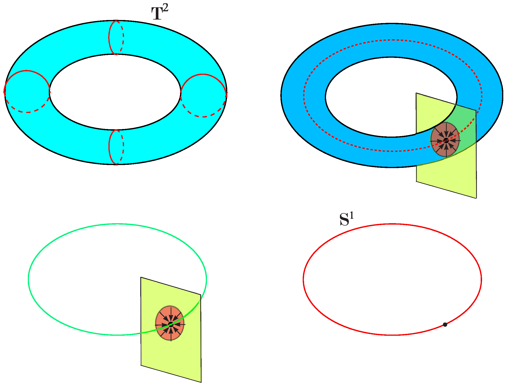
The tangent bundle of the real line coincides with ${\mathbb{R}}^2$. The tangent bundle of the circle is obtained by considering all tangent spaces (Figure 16, top) and combining them disjointly into a smooth manifold (Figure 16, bottom).

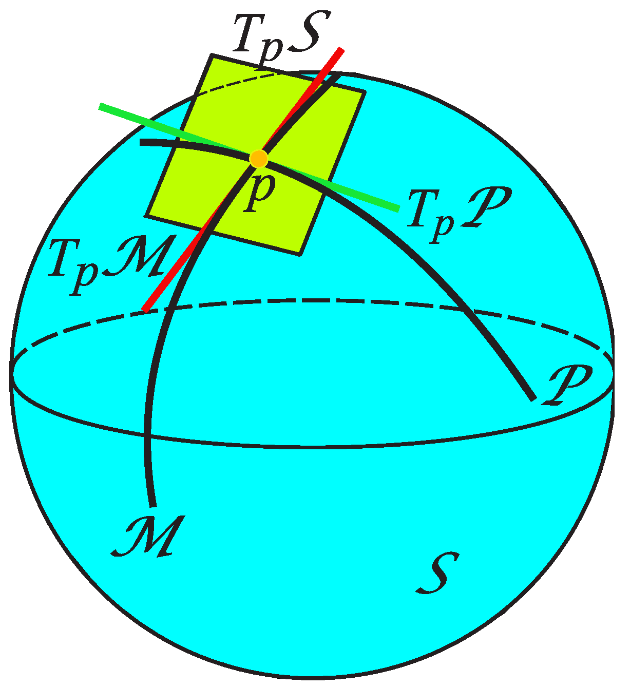
The map $\pi :T\mathcal{M}\to \mathcal{M}$, which assigns to each tangent vector $v\in T_p\mathcal{M}$ the base point $p\in \mathcal{M}$, at which the vector is tangent to $\mathcal{M}$, is called the natural projection. The preimage of a point $p\in \mathcal{M}$ under the natural projection, ${\pi }^{-1}\left(p\right)$, is the tangent space $T_p\mathcal{M}$. This space is called the fiber of the bundle over the point p.

Let $\mathcal{M}$ be a smooth manifold. Let us define the disjoint union of all normal spaces of $\mathcal{M}$,

$$N\mathcal{M}=\bigcup _{p\in \mathcal{M}}{N}_p\mathcal{M}.$$

The set $N\mathcal{M}$ is called normal bundle. The normal bundle of a circle is shown in Figure 17.

Assume that $\mathcal{M}\subseteq {\mathbb{R}}^n$ is an m-dimensional submanifold. The normal bundle $N\mathcal{M}$ consists of all vectors that are normal to $\mathcal{M}$:

$$N\mathcal{M}=\left\{(p,v)\in {\mathbb{R}}^n\times {\mathbb{R}}^n:p\in \mathcal{M},v\in N_p\mathcal{M}\right\}.$$

In this case, $N\mathcal{M}$ can be viewed as an n-dimensional submanifold of the Cartesian product ${\mathbb{R}}^n\times {\mathbb{R}}^n$.

Let $\mathcal{M}\subseteq {\mathbb{R}}^n$ be an m-dimensional submanifold without boundary. Then $N\mathcal{M}$ is a smooth manifold of dimension n.

Normal bundles can be considered more generally when we have a submanifold $\mathcal{P}\subset \mathcal{M}$, in order to understand the geometry of $\mathcal{P}$ within $\mathcal{M}$.

Definition 8 

(Normal bundle of a submanifold). Let $\mathcal{M}\subset {\mathbb{R}}^m$ be a manifold without boundary, and let $\mathcal{P}$ be a submanifold of $\mathcal{M}$. The normal bundle of $\mathcal{P}$ in $\mathcal{M}$ is defined as the set

$$N(\mathcal{P},\mathcal{M}):=\left\{(p,v):p\in \mathcal{P},v\in T_p\mathcal{M}andv\perp T_p\mathcal{P}\right\}.$$

The normal bundle $N(\mathcal{P},\mathcal{M})$ is a smooth manifold of dimension equal to $\dim \left(\mathcal{M}\right)$.

2.6. Tubular Neighborhoods

In this section we consider an important application of normal bundles, which is characterized by the fact that every smooth manifold $\mathcal{M}$ without boundary possesses a special type of neighborhood in the ambient space.

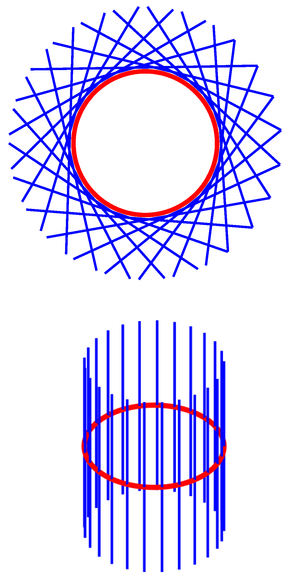
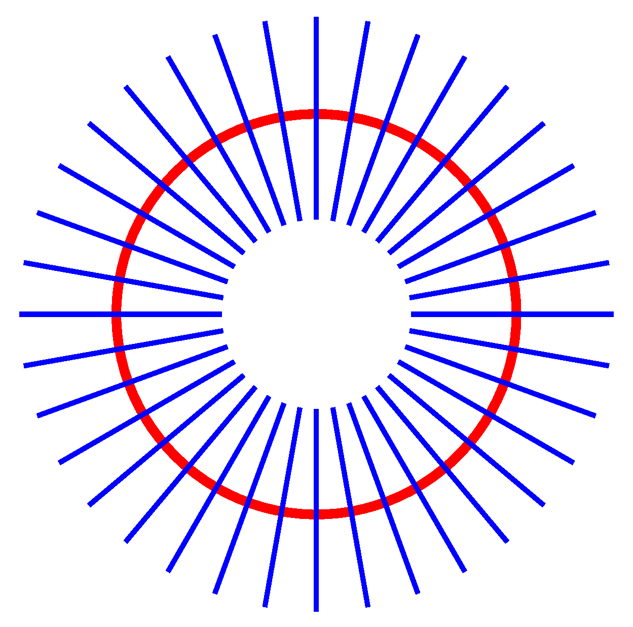
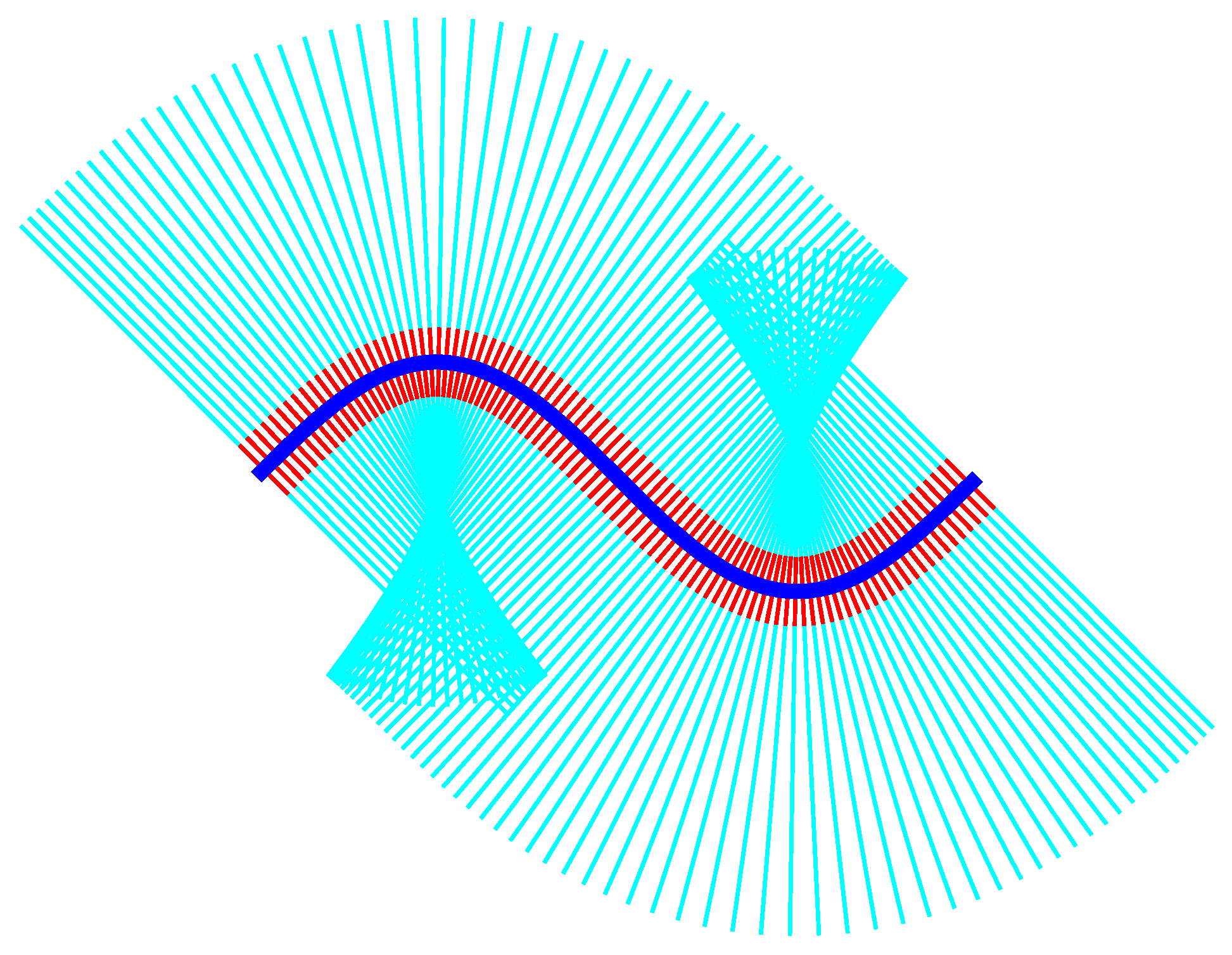
Generally speaking, a tubular neighborhood U of a smooth submanifold $\mathcal{M}$ is an open set around the submanifold whose structure resembles that of the normal bundle. This definition can be made more concrete by the following example. Let us consider a smooth plane curve without self-intersections. At each point of the curve we draw a straight line perpendicular to the curve. Except in the trivial case where the manifold is a straight line, these lines will intersect in a complicated way (Figure 18). However, if we consider a narrow strip around the curve, the portions of the normal lines contained in this strip will not intersect and will cover the entire strip without gaps.

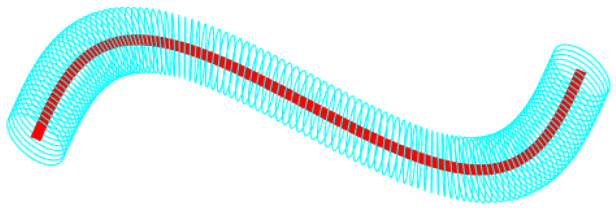
The tubular neighborhood of a space curve in ${\mathbb{R}}^3$ is shown in Figure 19.

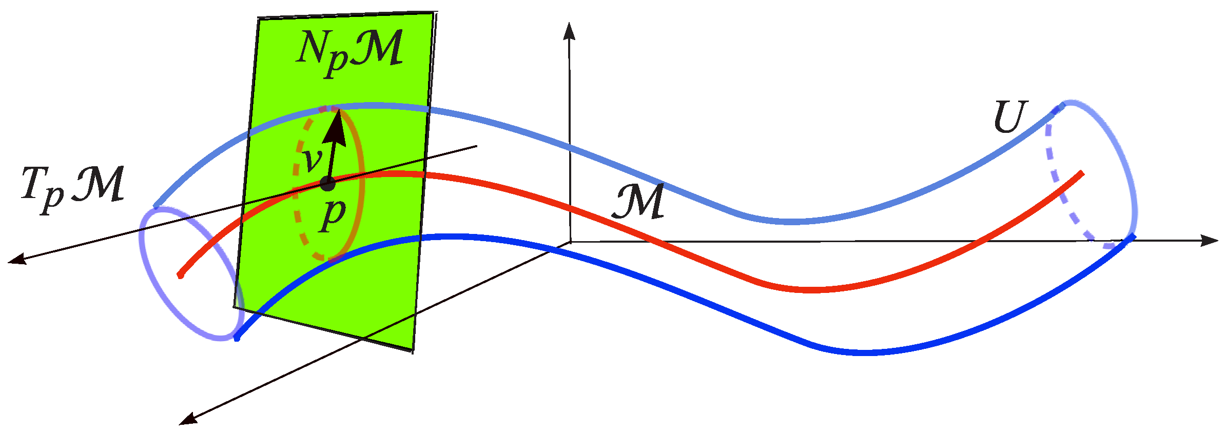
Let $\mathcal{M}\subseteq {\mathbb{R}}^n$ be an m-dimensional submanifold. Viewing the normal bundle $N\mathcal{M}$ as a submanifold of ${\mathbb{R}}^n\times {\mathbb{R}}^n$, we define the smooth map

$$E:N\mathcal{M}\to {\mathbb{R}}^n,(p,v)\mapsto p+v.$$

It maps each normal space $N_p\mathcal{M}$ affinely via p and orthogonally to $T_p\mathcal{M}$. The tubular neighborhood of $\mathcal{M}$ is the neighborhood U of $\mathcal{M}$ in ${\mathbb{R}}^n$ which is the diffeomorphic image, under this map, of an open subset $V\subset N\mathcal{M}$ of the form

$$V=\left\{(p,v)\in N\mathcal{M}:\left|v\right|<\epsilon \left(p\right)\right\},$$

for some smooth function $\epsilon :\mathcal{M}\to {\mathbb{R}}^{+}$ (Figure 20). We have the following definition:

Definition 9 

(Tubular neighborhood). Let $\mathcal{M}\subset {\mathbb{R}}^n$ be a smooth manifold without boundary. A tubular neighborhood of $\mathcal{M}$ is an open subset U of ${\mathbb{R}}^n$ containing $\mathcal{M}$ such that E maps an open subspace $V\subset N\mathcal{M}$ diffeomorphically onto U, where V is defined by a smooth function $\epsilon :\mathcal{M}\to {\mathbb{R}}^{+}$.

The key property of smooth manifolds embedded in a Euclidean space is that they always possess a tubular neighborhood.

Theorem 2. 

Every embedded submanifold of ${\mathbb{R}}^n$ has a tubular neighborhood.

Tubular neighborhoods and their properties are studied in detail in (Ch. 6, [5]), (Ch. 6, [10]), (Ch. 5, [13]).

2.7. Singular and Regular Points

Definition 10. 

Let f be a smooth map from an m-dimensional manifold $\mathcal{M}$ to an n-dimensional manifold $\mathcal{P}$.

(a)

A point $p\in \mathcal{M}$ is called critical or singular point of f if the derivative $D_{p}f:T_p\mathcal{M}\to T_{f\left(p\right)}\mathcal{P}$ is not surjective; that is, if $\mathrm{rank}\left(D_{p}f\right)<n$. The image $f\left(p\right)$ of a critical point is called a critical value of f.

(b)

A point $p\in \mathcal{M}$ is called a regular point of f if it is not critical. A point $q\in \mathcal{P}$ is called a regular value of f if its inverse image $f^{-1}\left(q\right)$ contains no critical points.

Note that if the dimension of $\mathcal{M}$ is smaller than the dimension of $\mathcal{P}$, then all points of $\mathcal{M}$ are critical points of f. On the other hand, if $f\left(\mathcal{M}\right)\ne \mathcal{P}$, then every point in $\mathcal{P}\setminus f\left(\mathcal{M}\right)$ is trivially a regular value, since its preimage is empty.

Example 5. 

(a)

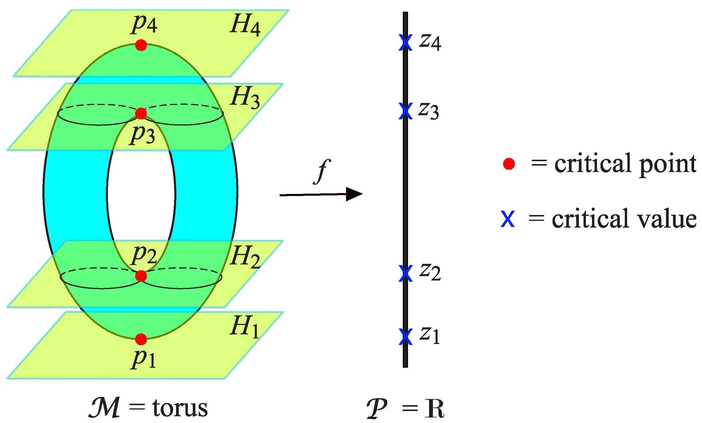
Let $\mathcal{M}$ be a torus embedded as a submanifold in three-dimensional Euclidean space. As illustrated in Figure 21, there exist exactly four horizontal planes (that is, planes of the form $z=\mathrm{const}$), denoted $H_1,H_2,H_3,H_4$, which are tangent planes to $\mathcal{M}$ at the points $p_1,p_2,p_3,p_4$, respectively. This corresponds to the fact that the function z restricted to $\mathcal{M}$ has critical points at $p_1,p_2,p_3,p_4$. These critical points correspond to the critical values $z_1=f\left(p_1\right),z_2=f\left(p_2\right),z_3=f\left(p_3\right),z_4=f\left(p_4\right)$.

(b)

Let $f:{\mathbb{R}}^{n+1}\to \mathbb{R}$ be the mapping

$$f\left(x\right)={\parallel x\parallel }^2=\sum _{i=1}^{n+1}{\left(x^i\right)}^2.$$

The derivative $D_{x}f$ at point $x=(x^1,\dots ,x^{n+1})$ is the linear mapping given, in the standard basis, by the matrix $(2x^1,\dots ,2x^{n+1})$. Thus, $D_{x}f:{\mathbb{R}}^{n+1}\to \mathbb{R}$ is surjective unless $x=0$, so every nonzero real number is a regular value of f. In particular, we obtain the sphere ${\mathbb{S}}^n=f^{-1}\left(1\right)$ as an n-dimensional manifold.

(c)

We consider the case in which the full-rank condition for the Jacobian matrix is not satisfied. Let the manifold $\mathcal{M}\subset {\mathbb{R}}^3$ be defined by the equation ${x^1}^2-{x^2}^2-{x^3}^2=0$ (see Figure 22). On the set $\mathcal{M}\setminus 0$, a structure of a two-dimensional $C^{\infty }$ submanifold can be defined. At the point 0, all minors of the Jacobian matrix vanish and its rank is not maximal. Therefore, the set $\mathcal{M}$ is an algebraic variety [25], and the point 0 is a singular point of this variety.

The study of abrupt changes that arise in families of objects depending smoothly on parameters is the subject of singularity theory [26,27,28,29]. This theory deals with the classification of types of changes and the characterization of the sets of parameters that give rise to sudden transitions. As the French mathematician Bernard Teissier says: I claim that Singularity Theory sits inside Mathematics much as Mathematics sits inside the general scientific culture …But singularity theory is also, again in a role played by Mathematics in general science, a crucible where different types of mathematical problems interact and surprising connections are born [30].

Singularity theory forms the foundation of the famous catastrophe theory [31,32,33,34,35,36].

2.8. Sard’s Theorem and Morse Functions

Theorem 3 

(Sard’s Theorem). Suppose that $\mathcal{M}$ and $\mathcal{P}$ are smooth manifolds and $f:\mathcal{M}\to \mathcal{P}$ is a smooth map. Then the set of critical values of f has measure zero in $\mathcal{P}$.

The proof of Theorem 3 can be found in (Ch. 1, [10]).

The following result shows that almost every point in the image of a smooth map is a regular value.

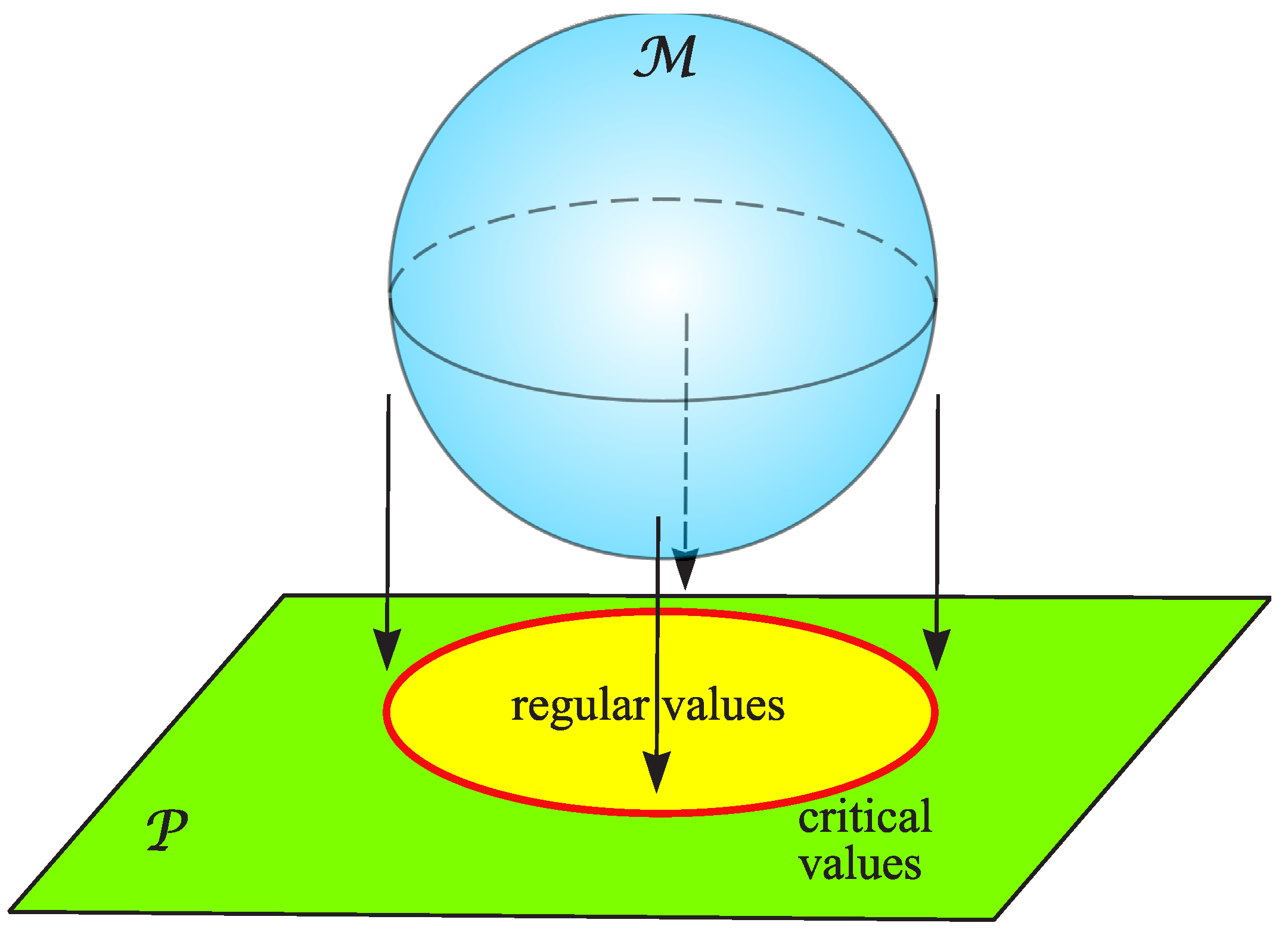
Sard’s Theorem is illustrated in Figure 23. This theorem is a key result in differential topology and is applied in many situations. For example, it is crucial for Thom’s Transversality Theorem (see Theorem 4).

An equivalent formulation of Sard’s Theorem is as follows:

If $f:\mathcal{M}\to \mathcal{P}$ is a smooth map between manifolds, then almost every $y\in \mathcal{P}$ (in the sense of measure) is a regular value of f; equivalently, the set of critical values has measure zero.

It should be emphasized that this theorem refers to regular values, not regular points. For example, a constant function of one variable has no regular points (all points are critical), but it has only one critical value, so the remaining points in $\mathbb{R}$ are regular values. A set consisting of a single point clearly has measure zero.

Sard’s theorem was published by the American mathematician Arthur Sard in 1942.

It is interesting to study the behavior of a function f near its critical points. If $\mathcal{M}$ is a compact set, every function on it must have a maximum and a minimum. However, if $f\left(x\right)$ has an extremum, its derivative $D_{x}f$ must be equal to zero. Thus, over a compact connected manifold without boundary, every smooth function has at least two critical points (except in the case $\mathcal{M}=\left\{\text{a} \text{single} \text{point}\right\}$).

Let $f:{\mathbb{R}}^k\to \mathbb{R}$ be a smooth function. Locally, near a point $c\in {\mathbb{R}}^k$, f admits the Taylor series expansion

$$f\left(x\right)=f\left(c\right)+\sum _{i=1}^k{\displaystyle \frac{\partial f}{\partial x^i}}\left(c\right)·(x^i-c^i)+{\displaystyle \frac{1}{2}}\sum _{i,j=1}^k{\displaystyle \frac{{\partial }^{2}f}{\partial x^i\partial x^j}}\left(c\right)·(x^i-c^i)(x^j-c^j){+o\left(\right|x-c|}^2).$$

(2)

If c is a critical point, then by definition:

$$D_{c}f=\left({\displaystyle \frac{\partial f}{\partial x^1}}\left(c\right),\dots ,{\displaystyle \frac{\partial f}{\partial x^k}}\left(c\right)\right)=(0,\dots ,0).$$

Hence, in the neighborhood of a critical point, the terms that are linear in $x^i-c^i$ vanish. The leading contribution to the local behavior of f at c is therefore given by the quadratic term, which is determined by the Hessian matrix of second derivatives:

$$H\left(c\right)=\left[{\displaystyle \frac{{\partial }^{2}f}{\partial x^i\partial x^j}}\right].$$

Note that the Hessian $H\left(c\right)$ is a real symmetric matrix and therefore has only real eigenvalues. If all eigenvalues of $H\left(c\right)$ are positive, then $H\left(c\right)$ is positive definite and f has a (strict) local minimum at c. If all eigenvalues are negative, then $H\left(c\right)$ is negative definite and f has a (strict) local maximum at c.

If the Hessian has both positive and negative eigenvalues, then c is a saddle point.

Definition 11 

(Non-degenerate critical points and Morse functions). For a smooth function $f:{\mathbb{R}}^k\to \mathbb{R}$, a point $c\in {\mathbb{R}}^k$ where $D_{c}f=0$ but the Hessian matrix

$$H_c\left(f\right)=\left[{\displaystyle \frac{{\partial }^{2}f}{\partial x^i\partial x^j}}\left(c\right)\right]$$

is invertible at c, is called a non-degenerate critical point of f. If all critical points of f are non-degenerate, then f is called a non-degenerate function or Morse function.

The local behavior of a function at a nondegenerate critical point is completely determined, up to a diffeomorphism, by the following theorem.

Lemma 1 

(Morse Lemma). Let $\mathcal{M}$ be a smooth k-dimensional manifold and let $f:\mathcal{M}\to \mathbb{R}$ be a smooth function. Suppose that a point $c\in \mathcal{M}$ is a nondegenerate critical point of f, and let

$$\left[{\displaystyle \frac{{\partial }^{2}f}{\partial x^i\partial x^j}}\left(c\right)\right]$$

be the Hessian of f at c. Then there exists a local coordinate system $(x^1,\dots ,x^k)$ in a neighborhood of c such that

$$f=f\left(c\right)-{x^1}^2-\dots -{x^s}^2+{x^{s+1}}^2+\dots +{x^k}^2,$$

where s is the number of negative eigenvalues of the Hessian of f at c.

Morse’s lemma was published by the American mathematician Marston Morse in 1925.

Example 6. 

In this example, we consider a matrix for which we are interested in the local behavior of the map $\det :{\mathbb{R}}^2\to \mathbb{R}$ in the neighborhood of a singular point of the map.

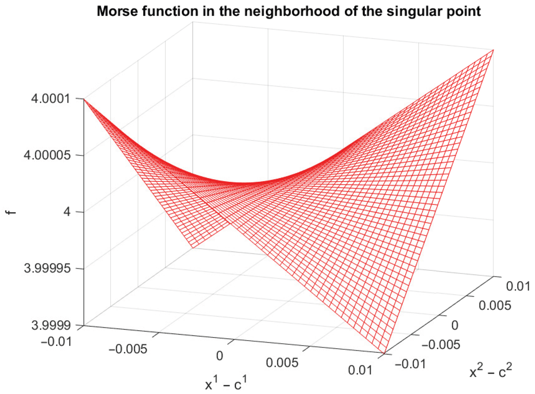
Consider the matrix

$$A=\left[\begin{array}{cc}{x}^1-2& x^1\\ -2& x^2-1\end{array}\right],$$

whose entries depend on the parameters $x^1$ and $x^2$.

We have

$$f=\det \left(A\right)=x^1-2x^2+x^1{x}^2+2$$

and

$$Df=\left[{\displaystyle \frac{\partial f}{\partial x^1}},{\displaystyle \frac{\partial f}{\partial x^2}}\right]=[x^2+1,x^1-2].$$

It is clear that $Df$ is surjective whenever $(x^2+1,x^1-2)\ne (0,0)$, i.e., except at the point

$$c=[2,-1]$$

where $Df$ vanishes. At this point, the function f takes the value 4.

The Hessian matrix in this case is

$$H=\left[\begin{array}{cc}{\displaystyle \frac{{\partial }^{2}f}{{\partial }^2{x}^1}}& {\displaystyle \frac{{\partial }^{2}f}{\partial x^1\partial x^2}}\\ {\displaystyle \frac{{\partial }^{2}f}{\partial x^1\partial x^2}}& {\displaystyle \frac{{\partial }^{2}f}{{\partial }^2{x}^2}}\end{array}\right]=\left[\begin{array}{cc}0& 1\\ 1& 0\end{array}\right].$$

This matrix is non-singular, which means that the critical point is non-degenerate. The eigenvalues of the Hessian are −1 and 1. In local coordinates centered at $c=[2,-1]$, the quadratic part of f is $x^1{x}^2$.

By performing a change of coordinates via the non-singular transformation $x=Uy$, where

$$U=\left[\begin{array}{cc}\hfill 1& \hfill 1\\ \hfill -1& \hfill 1\end{array}\right],$$

we obtain $U^{-1}HU=\mathrm{diag}(-1,1)$ and

$$x^1=y^1+y^2,x^2=-y^1+y^2.$$

According to Morse’s lemma, the function f can then be expressed near the singular point as

$$f\left(y\right)=f\left(c\right)-{y^1}^2+{y^2}^2.$$

This function has the shape of a “saddle point”, due to the presence of both a positive and a negative eigenvalue of the Hessian (Figure 24).

Computations in the neighbourhood of algebraic singularities are considered in [37].

2.9. Transverse Intersection of Manifolds

Let $\mathcal{M}$ and $\mathcal{P}$ be smooth submanifolds of an ambient manifold $\mathcal{S}$. They are said to intersect transversally if for every $x\in \mathcal{M}\cap \mathcal{P}$, their tangent spaces at x satisfy

$$T_{\mathcal{M}}\left(x\right)+T_{\mathcal{P}}\left(x\right)=T_{\mathcal{S}}\left(x\right).$$

(Figure 25). That is, the directions tangent to $\mathcal{M}$ together with the directions tangent to $\mathcal{P}$ span all possible directions of the ambient manifold.

The term frequently used synonymously for transversal is general position, i.e., two manifolds which intersect transversally are said to be in general position.

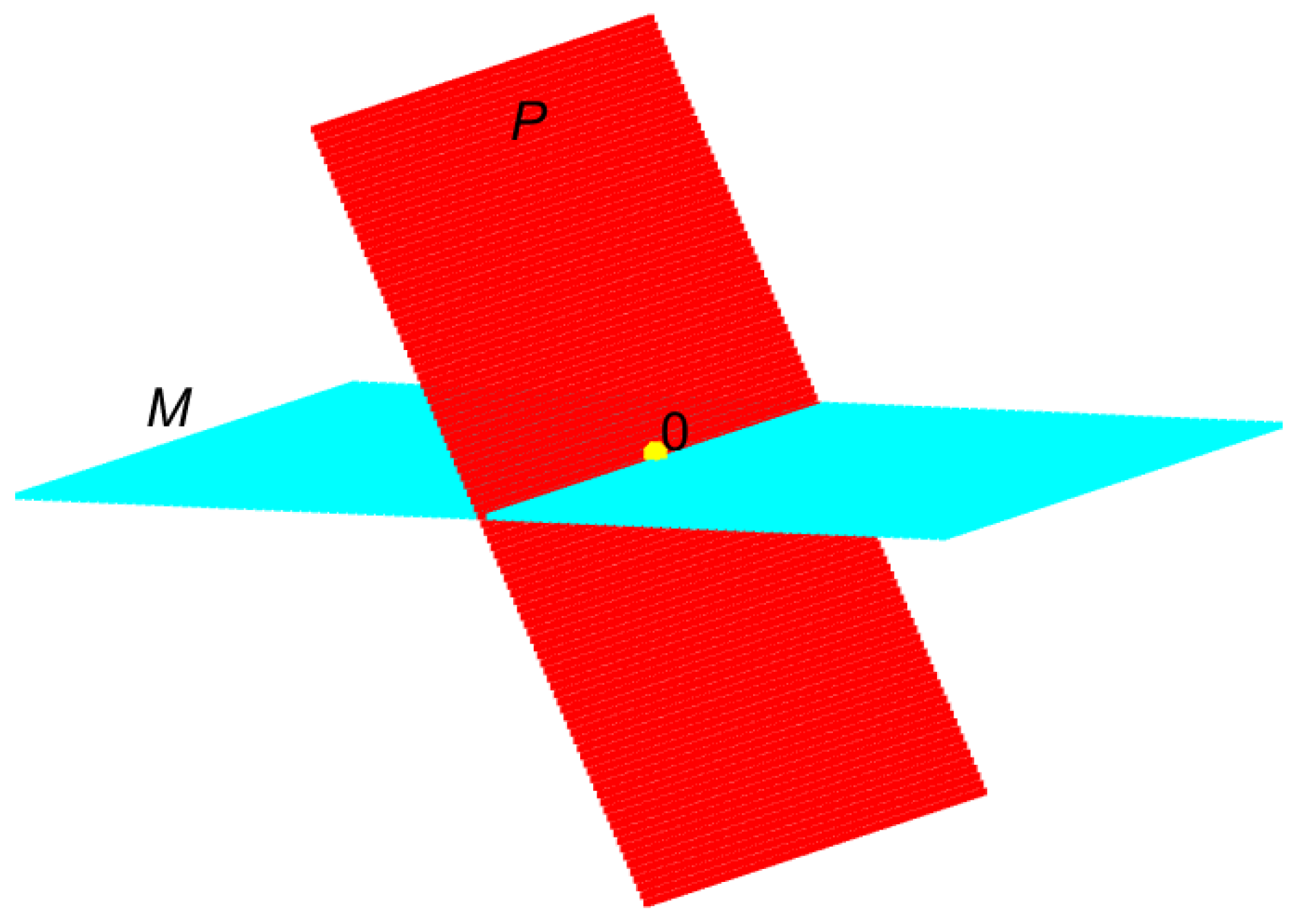
Two linear subspaces $\mathcal{X}$ and $\mathcal{Y}$ of a linear space $\mathcal{L}$ are transverse, if their sum is equal to the whole space, $\mathcal{X}+\mathcal{Y}=\mathcal{L}$. For instance, two planes intersecting at nonzero angles in ${\mathbb{R}}^3$ are transverse (Figure 26).

In three-dimensional space, transverse curves do not intersect. Indeed, if ${\mathcal{C}}_1$ and ${\mathcal{C}}_2$ are curves in ${\mathbb{R}}^3$, then

$$dim{\mathcal{C}}_1+dim{\mathcal{C}}_2=1+1<3,$$

so their tangent spaces cannot span the tangent space of the ambient manifold at a common point.

A curve transverse to a surface intersects the surface in isolated points. In this case

$$dim\mathcal{C}+dim\mathcal{S}=1+2=3,$$

and transversality implies that at each intersection point the tangent line to the curve together with the tangent plane to the surface span ${\mathbb{R}}^3$.

Similarly, two surfaces transverse to each other intersect in a curve. Indeed,

$$dim{\mathcal{S}}_1+dim{\mathcal{S}}_2=2+2>3,$$

and their transverse intersection has dimension

$$2+2-3=1.$$

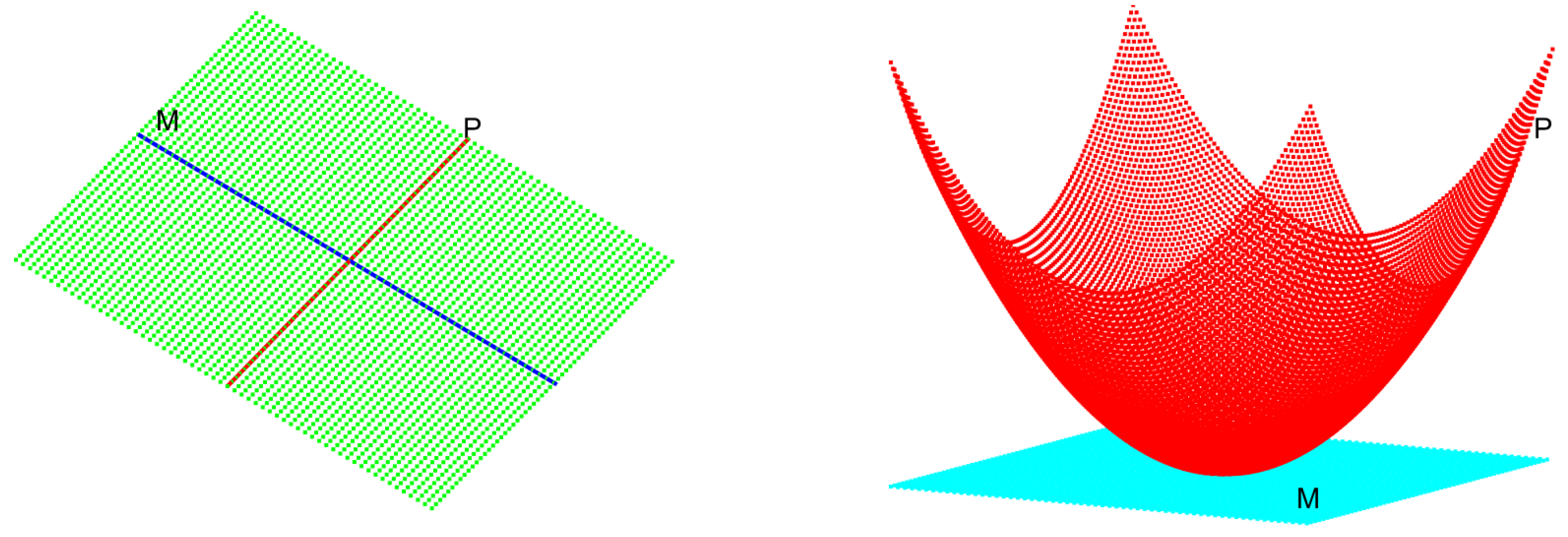
Note that two perpendicular planes in ${\mathbb{R}}^3$ intersect transversally, whereas two perpendicular lines lying in one and the same plane do not (Figure 27, left). Curves that are tangent to a surface at a point (for example, curves lying entirely on a surface) do not intersect the surface transversally. The same is true for planes that are tangent to a surface at a point (Figure 27, right). If an intersection of two submanifolds is transverse, then it is itself a smooth submanifold whose codimension is equal to the sums of the codimensions of the two intersecting manifolds.

The following result shows that transverse intersections are generic among intersections of smooth manifolds.

Theorem 4 

(Thom’s Transversality Theorem (Ch. 2, [3])). Suppose we have a family of smooth maps

$$f_s:\mathcal{M}\to \mathcal{P},f_s\left(x\right)=F(x,s),$$

where each map depends smoothly on a parameter s belonging to a parameter space $\mathcal{S}$. Assume that $\mathcal{M}$ may have a boundary, while $\mathcal{P}$ and a given submanifold $\mathcal{Z}\subset \mathcal{P}$ do not.

If the full mapping $F(x,s)$, as well as its restriction to the boundary of $\mathcal{M}$, intersects $\mathcal{Z}$ in a transversal way, then for “almost all” choices of the parameter s the corresponding map $f_s\left(x\right)$ also intersects $\mathcal{Z}$ transversally, both in the interior of $\mathcal{M}$ and on its boundary.

In other words, transversality is a generic property: although a particular map may fail to be transversal, a small perturbation—obtained by slightly changing the parameter s—will typically restore transversality.

The concept of transversality was developed by the French mathematician René Thom in the 1950s.

2.10. Lie Groups

Lie groups are among the most powerful tools of differential topology, applied in a variety of areas, such as the theory of differential equations, the study of special functions, and matrix analysis. In this section, some basic information about Lie groups and their properties is provided.

A clear introduction to matrix groups and the Lie algebra is given in [38]. The theory of Lie groups and Lie algebras is presented in depth in (Ch. 7, [5]), (Ch. 4, [9]), [39], (Ch.3, [40]). A comprehensive overview of Lie group theory, matrix Lie groups, and matrix Lie algebras is given in [41]. The group-theoretic approach to matrices and vector spaces is developed in detail in [42]. Applications of Lie groups in the theory of differential equations are discussed in [43].

2.10.1. Basic Definitions

Definition 12. 

A group is a set G together with a group operation, usually called multiplication, such that for any two elements $g,h\in G$, their product $g·h$ is again an element of G. The group operation is required to satisfy the following properties:

(1)

Associativity. If g, h, and k are elements of G, then

$$g·(h·k)=(g·h)·k.$$

(2)

Existence of an identity element. There exists a distinguished element $e\in G$, called the identity element, which satisfies

$$e·g=g·e=g$$

for all $g\in G$.

(3)

Existence of an inverse element. For every $g\in G$, there exists an inverse element, denoted $g^{-1}$, which satisfies

$$g·g^{-1}=e=g^{-1}·g.$$

Below are some elementary examples of groups.

Example 7. 

(a)

Let $G=\mathbb{Z}$ be the set of integers with the group operation being addition. Clearly, associativity holds, the identity element is 0, and the “inverse” of an integer x is $-x$.

(b)

Similarly, $G=\mathbb{R}$—the set of real numbers—is also a group under addition. Again, the identity element is 0, and the inverse of a real number x is $-x$. In both cases, the group operation is commutative: $g·h=h·g$ for all $g,h\in G$. Such groups are called Abelian.

(c)

Let $G=GL(n,\mathbb{Q})$ be the set of invertible $n\times n$ matrices with rational entries. The group operation is matrix multiplication. The identity element is the identity matrix I, and the inverse of a matrix A is the usual inverse matrix, whose entries are again rational numbers.

(d)

Similarly, the general linear group $GL(n,\mathbb{R})$—the set of invertible $n\times n$ matrices with real entries—is a group under matrix multiplication with the same identity element and inverses as in the previous example.

Lie groups are smooth manifolds that are also groups, in which the multiplication and inversion operations are smooth maps. Besides providing many interesting examples of manifolds in their own right, Lie groups are a fundamental tool in the study of more general manifolds.

In examples (b) and (d) given above, we actually have Lie groups, since the sets $\mathbb{R}$ and $GL\left(n\right)$ are smooth manifolds. In both cases, the group operation is smooth (in fact, analytic). This leads to the following general definition of a Lie group.

Definition 13 

(Lie Groups). A Lie group is a smooth manifold G that is also a group in the algebraic sense, with the property that the multiplication map $m:G\times G\to G$ and the inverse map $i:G\to G$, defined by

$$m(g,h)=g·h,i\left(g\right)=g^{-1},$$

are both smooth maps of manifolds.

Every Lie group is a topological group, that is, a topological space equipped with a group structure such that the multiplication and inversion maps are continuous.

In fact, one can equivalently state that if G is a smooth manifold with a group structure such that the map

$$G\times G\to G,(g,h)\mapsto g{h}^{-1}$$

is smooth, then G is a Lie group.

Lie groups lie at the boundary between algebra and topology. The algebraic properties of Lie groups follow from the group axioms, while their geometric properties arise from the parametrization of group elements by points of a differentiable manifold. At the topological level, a Lie group is homogeneous, meaning that every point of the manifold parametrizing the group looks the same as any other point.

The dimension of a Lie group is the dimension of the manifold that parametrizes the group operations. If G is an r-dimensional smooth manifold, the corresponding Lie group is also called an r-parameter Lie group.

If G is a Lie group, any element $g\in G$ defines the maps $L_g,R_g:G\to G$, called respectively the left translation and right translation, given by

$$L_g\left(h\right)=gh,R_g\left(h\right)=hg.$$

The maps $L_g$ and $R_g$ are smooth and, in fact, are diffeomorphisms of G.

Example 8 

(Lie Groups). Each of the following manifolds is a Lie group with the specified group operation.

(a)

The general linear group $GL(n,\mathbb{R})$ is the set of all invertible $n\times n$ matrices with real entries. It is a group with group operation given by matrix multiplication, as already noted in Example 7(d), and it is an open subset of the vector space $\mathcal{M}(n,\mathbb{R})$. As will be shown below, multiplication is smooth since the entries of the matrix product $AB$ are polynomials in the entries of A and B.

(b)

Let $G{L}^{+}(n,\mathbb{R})$ denote the subset of $GL(n,\mathbb{R})$ consisting of matrices with positive determinant. Since $det\left(AB\right)=det\left(A\right)det\left(B\right)$ and $det\left(A^{-1}\right)=1/det\left(A\right)$, it is a subgroup of $GL(n,\mathbb{R})$. Because this subset is the preimage of $(0,\infty )$ under the continuous determinant function, it is an open subset of $GL(n,\mathbb{R})$ and hence an $n^2$-dimensional manifold. The group operations are the restrictions of those on $GL(n,\mathbb{R})$ and are therefore smooth. Thus $G{L}^{+}(n,\mathbb{R})$ is a Lie group.

(c)

The complex general linear group $GL(n,\mathbb{C})$ is the group of invertible complex $n\times n$ matrices under matrix multiplication. It is an open submanifold of $\mathcal{M}(n,\mathbb{C})$ and hence a $2n^2$-dimensional smooth manifold. It is a Lie group since matrix multiplication and inversion are smooth functions of the real and imaginary parts of the matrix entries.

(d)

If V is an arbitrary real or complex vector space, $GL\left(V\right)$ denotes the set of invertible linear transformations from V to itself. It is a group under composition of functions. If V has finite dimension n, any choice of basis of V determines an isomorphism of $GL\left(V\right)$ with $GL(n,\mathbb{R})$ or $GL(n,\mathbb{C})$, so that $GL\left(V\right)$ is a Lie group. The transition map between two such isomorphisms is given by a map of the form $A\mapsto BA{B}^{-1}$, where B is the change-of-basis matrix, which is smooth. Consequently, the smooth manifold structure on $GL\left(V\right)$ is independent of the choice of basis.

(e)

The field of real numbers $\mathbb{R}$ is a Lie group under addition, with the inverse given by $x\mapsto -x$.

(f)

Let $G={\mathbb{R}}^r$ with its natural manifold structure, and let the group operation be vector addition $(x,y)\mapsto x+y$. The inverse of a vector x is $-x$. These operations are smooth, so ${\mathbb{R}}^r$ provides an example of an r-parameter Abelian Lie group. Similarly, $\mathbb{C}$ and ${\mathbb{C}}^n$ are Lie groups under addition.

(g)

Let $G=SO\left(2\right)$ be the group of planar rotations. That is,

$$G=\left\{\left[\begin{array}{cc}cos\theta & -sin\theta \\ sin\theta & cos\theta \end{array}\right]:0\le \theta <2\pi \right\},$$

where θ denotes the angle of rotation of a vector under multiplication by the rotation matrix. Note that G can be identified with the unit circle

$${\mathbb{S}}^1=\left\{(cos\theta ,sin\theta ):0\le \theta <2\pi \right\}$$

in ${\mathbb{R}}^2$, which allows one to endow $SO\left(2\right)$ with a manifold structure.

2.10.2. Matrix Groups

In this section we consider several matrix Lie groups that play an important role in matrix analysis and matrix computations. For brevity, in what follows we shall denote the general linear group $GL(n,\mathbb{R})$ simply by $GL\left(n\right)$.

• General linear group
  As noted above, the general linear group

  $$GL\left(n\right)=\left\{A\in \mathcal{M}\left(n\right):det\left(A\right)\ne 0\right\}$$

  consisting of all invertible $n\times n$ matrices with real entries is a smooth manifold of dimension $n^2$, since it is an open subset of the space of all $n\times n$ matrices $\mathcal{M}\left(n\right)$. Indeed,

  $$GL\left(n\right)={\mathbb{R}}^{n^2}\setminus \left\{det\left(A\right)=0\right\},$$

  where the space ${\mathbb{R}}^{n^2}$ is identified with the space $\mathcal{M}\left(n\right)$ of all real $n\times n$ matrices. Since the determinant function $det:\mathcal{M}\left(n\right)\to \mathbb{R}$ is continuous (because $det\left(A\right)$ is a polynomial in the matrix entries) the set ${\mathbb{R}}^{n^2}\setminus \left\{det\left(A\right)=0\right\}$ is open. Hence it is a smooth manifold of dimension $n^2$.
  To prove that $GL\left(n\right)$ is a Lie group, we must verify that matrix multiplication and matrix inversion are smooth operations. Given two matrices A and B in $GL\left(n\right)$, the element in position $(i,j)$ of the product $AB$ is given by

  $${\left(AB\right)}_{ij}=\sum _{k=1}^n{a}_{ik}{b}_{kj}.$$
  Thus, ${\left(AB\right)}_{ij}$ is a polynomial of degree two in the entries of A and B. Consequently, the matrix multiplication map

  $$m:GL\left(n\right)\times GL\left(n\right)\to GL\left(n\right)$$

  is a smooth mapping.
  Recall that the $\left(ij\right)$-minor of a matrix A is the determinant of the submatrix $A_{ij}$, obtained by deleting the i-th row and the j-th column of A. According to Cramer’s rule the $\left(ij\right)$-th entry of $A^{-1}$ is given by

  $${\left(A^{-1}\right)}_{ij}={\displaystyle \frac{{(-1)}^{i+j}}{det\left(A\right)}}(\mathrm{the}(j,i)-\mathrm{minor}\mathrm{of}A),$$

  which is a smooth function of the entries $a_{ij}$, provided that $det\left(A\right)\ne 0$. That is, the mapping

  $$\mathcal{M}\left(n\right)\to \mathbb{R},A\mapsto {\left(A^{-1}\right)}_{ij}$$

  is smooth, since it depends smoothly on the entries of A. Therefore, the matrix inversion map

  $$i:GL\left(n\right)\to GL\left(n\right)$$

  is also smooth.
  The complex general linear group $GL(n,\mathbb{C})$ is likewise a Lie group with respect to matrix multiplication and inversion. The set $GL(n,\mathbb{C})$ is an open subset of $M(n,\mathbb{C})$ and hence is a smooth manifold of dimension $2n^2$. It is a Lie group because matrix multiplication and inversion are smooth functions of the real and imaginary parts of the matrix entries.
• Special Linear Group
  This group is defined as

  $$SL\left(n\right)=\left\{A\in \mathcal{M}\left(n\right):det\left(A\right)=1\right\}.$$
  Geometrically, $SL\left(n\right)$ consists of all transformations of ${\mathbb{R}}^n$ that preserve both volume and orientation. It can be shown that $SL\left(n\right)={det}^{-1}\left(1\right)$ is a smooth manifold of dimension $n^2-1$, defined by the condition $det\left(A\right)-1=0$. Since this manifold is a subset of the Lie group $GL\left(n\right)$ with the operation inherited from $GL\left(n\right)$, $SL\left(n\right)$ is also a Lie group. Moreover, the tangent space of $SL\left(n\right)$ at the identity is the subspace of $\mathcal{M}(n,\mathbb{R})$ consisting of all matrices with zero trace.
• Group of Orthogonal Matrices
  The group of orthogonal $n\times n$ matrices is defined as

  $$O\left(n\right)=\left\{A\in GL\left(n\right):A^{T}A=I_n\right\}.$$
  Thus, $O\left(n\right)$ is a subset of ${\mathbb{R}}^{n^2}$, defined by $n^2$ equations

  $$A^{T}A-I_n=0$$

  in terms of the entries $a_{ij}$ of the matrix A. It can be shown that exactly $n(n+1)/2$ of these equations, corresponding to the entries on and above the diagonal, are independent and satisfy the maximal rank condition for $O\left(n\right)$ everywhere. Therefore, $O\left(n\right)$ is a submanifold of $GL\left(n\right)$ of dimension $n^2-n(n+1)/2=n(n-1)/2$. Moreover, matrix multiplication and the matrix inversion operation remain smooth when restricted to $O\left(n\right)$. Consequently, $O\left(n\right)$ itself is a Lie group.
• Special Orthogonal Group
  The equation

  $$A^{T}A=I_n,$$

  used in the definition of the orthogonal group $O\left(n\right)$, in particular implies that every matrix $A\in O\left(n\right)$ is invertible with $A^{-1}=A^T$. Consequently, the determinant of $A\in O\left(n\right)$ must satisfy ${(det\left(A\right))}^2=1$, i.e., $det\left(A\right)=\pm 1$. In this way, $O\left(n\right)$ is divided into two disconnected components: the subset of matrices with determinant $+1$ and the subset of matrices with determinant $-1$.
  If A and B both have determinant −1, then their product $AB$ has determinant $+1$. Therefore, the subset of orthogonal matrices with determinant $-1$ is not closed under multiplication and is not a subgroup of $O\left(n\right)$. The other component, however, is a Lie subgroup of $O\left(n\right)$ and is called the special orthogonal group, denoted by $SO\left(n\right)$,

  $$SO\left(n\right)=\left\{A\in O\left(n\right):det\left(A\right)=1\right\}\subset O\left(n\right).$$
  The subgroup $SO\left(n\right)$ is a Lie group.
• Unitary and Special Unitary Groups
  The unitary group $U\left(n\right)$ is defined as

  $$U\left(n\right):=\left\{A\in GL(n,\mathbb{C}):A^{H}A=I_n\right\},$$

  where $A^H={\overline{A}}^T$ denotes the Hermitian (complex conjugate transpose) of A. A similar argument as for $O\left(n\right)$ shows that $U\left(n\right)$ is a submanifold of $GL(n,\mathbb{C})$ and that $\dim U\left(n\right)=n^2$.
  The special unitary group $SU\left(n\right)$ is defined as the subgroup of $U\left(n\right)$ consisting of matrices with determinant equal to 1.
• Group of Upper Unit Triangular Matrices
  The group $T\left(n\right)$ of upper triangular matrices with ones on the main diagonal is an $n(n-1)/2$-parameter Lie group. As a manifold, $T\left(n\right)$ can be identified with the Euclidean space ${\mathbb{R}}^{n(n-1)/2}$, since each matrix is uniquely determined by its entries above the diagonal. For example, in the case of $T\left(3\right)$ we identify the matrix

  $$\left[\begin{array}{ccc}1& x& z\\ 0& 1& y\\ 0& 0& 1\end{array}\right]\in T\left(3\right)$$

  with the vector $(x,y,z)$ in ${\mathbb{R}}^3$. However, except for the special case $T\left(2\right)$, the group $T\left(n\right)$ is not isomorphic to the Abelian Lie group ${\mathbb{R}}^{n(n-1)/2}$.

Several other important matrix groups are defined by imposing linear or quadratic constraints on the $n^2$ entries of $GL(n,\mathbb{F})$ or $SL(n,\mathbb{F})$.

2.10.3. Lie Algebra of a Lie Group

A Lie algebra (over $\mathbb{R}$) is a real vector space $\mathfrak{g}$, equipped with a mapping, called the bracket, from $\mathfrak{g}\times \mathfrak{g}$ to $\mathfrak{g}$, usually denoted by $(X,Y)\mapsto [X,Y]$, which satisfies the following properties for all $X,Y,Z\in \mathfrak{g}$:

(a)

Bilinearity: For $a,b\in \mathbb{R}$,

$$[aX+bY,Z]=a[X,Z]+b[Y,Z],$$

$$[Z,aX+bY]=a[Z,X]+b[Z,Y].$$

(b)

Antisymmetry:

$$[X,Y]=-[Y,X].$$

(c)

Jacobi identity:

$$[X,[Y,Z\left]\right]+[Y,[Z,X\left]\right]+[Z,[X,Y\left]\right]=0.$$

For a given Lie group, the Jacobi identity for its Lie algebra follows from the group structure via differentiation at the identity.

If $\mathfrak{g}$ is a Lie algebra, a linear subspace $\mathfrak{h}\subseteq \mathfrak{g}$ is called a Lie subalgebra of $\mathfrak{g}$, if it is closed under the bracket operation. In this case $\mathfrak{h}$ itself is a Lie algebra with the restriction of the same bracket.

If $\mathfrak{g}$ and $\mathfrak{h}$ are Lie algebras, a linear mapping $A:\mathfrak{g}\to \mathfrak{h}$ is called a Lie algebra homomorphism if it preserves brackets:

$$A[X,Y]=[AX,AY].$$

An invertible Lie algebra homomorphism is called a Lie algebra isomorphism.

Example 9 

(Lie algebras).

(a)

The vector space $\mathcal{M}(n,\mathbb{R})$ of all real matrices becomes an $n^2$-dimensional Lie algebra under the commutator bracket

$$[A,B]=AB-BA.$$

Bilinearity and antisymmetry are immediate from the definition, and the Jacobi identity follows from straightforward computations. When considered as a Lie algebra with this bracket, it is denoted by $\mathfrak{g}\mathfrak{l}(n,\mathbb{R})$.

(b)

Similarly, $\mathfrak{g}\mathfrak{l}(n,\mathbb{C})$ is the $2n^2$-dimensional (real) Lie algebra obtained by equipping complex matrices with the commutator bracket.

A simple example of a 3-dimensional Lie algebra over $\mathbb{C}$ is $\mathfrak{s}\mathfrak{l}(2,\mathbb{C})$, the space of $2\times 2$ matrices with zero trace. A basis of this space is given by

$$H=\left[\begin{array}{cc}1& 0\\ 0& -1\end{array}\right],E=\left[\begin{array}{cc}0& 1\\ 0& 0\end{array}\right],F=\left[\begin{array}{cc}0& 0\\ 1& 0\end{array}\right].$$

The commutators are

$$\begin{array}{ccc}& & [H,E]=HE-EH=2E,\hfill \\ & & [H,F]=HF-FH=-2F,\hfill \\ & & [E,F]=EF-FE=H.\hfill \end{array}$$

(c)

Any vector space V becomes a Lie algebra if all brackets are defined to be zero. Such Lie algebras are called abelian Lie algebras.

3. Geometry of Matrix Space

3.1. The Matrix Space

Let us consider the linear operator

$$\mathcal{A}:{\mathbb{F}}^n\to {\mathbb{F}}^m,$$

represented by a rectangular matrix $A\in {\mathbb{F}}^{m\times n}$, where $\mathbb{F}$ is $\mathbb{C}$ or $\mathbb{R}$. The finite-dimensional space of all linear operators from ${\mathbb{F}}^n$ to ${\mathbb{F}}^m$ is naturally isomorphic to the vector space ${\mathbb{F}}^{m·n}$, so the two spaces may be regarded as the same metric space. This makes it possible to study the space of linear operators using methods from the analysis of metric and topological spaces.

Let the set $\mathcal{M}(m,n)$ of all $m\times n$ matrices with entries in $\mathbb{F}$ be endowed with the topology induced by the natural mapping $i:{\mathbb{F}}^{m·n}\to M(m,n)$:

$$(x^1,x^2,\dots ,x^{mn})\mapsto \left[\begin{array}{cccc}{x}^1& x^2& \dots & x^n\\ x^{n+1}& x^{n+2}& \dots & x^{2n}\\ ⋮& ⋮& \ddots & ⋮\\ x^{(m-1)n+1}& x^{(m-1)n+2}& \dots & x^{mn}\end{array}\right].$$

When $\mathbb{F}=\mathbb{R}$ or $\mathbb{F}=\mathbb{C}$, the mapping i is a homeomorphism that induces on $\mathcal{M}(m,n)$ the structure of a smooth $\left(C^{\infty }\right)$ manifold of real dimension $mn$. In other words, the set $\mathcal{M}(m,n)$ of all rectangular matrices $A\in {\mathbb{F}}^{m\times n}$ forms a smooth manifold of dimension $m·n$, coinciding with the vector space ${\mathbb{F}}^{m·n}$.

According to the above considerations, a complex rectangular matrix $A\in {\mathbb{C}}^{m\times n}$ can be represented as a point in the complex linear space ${\mathbb{C}}^{m\times n}$ of dimension $m·n$; as a real manifold it has dimension $2mn$. Similarly, a real $m\times n$ matrix A can be viewed as a point in the real space ${\mathbb{R}}^N$, with $N=m·n$, by arranging its entries in a prescribed order and interpreting them as coordinates. The corresponding space is called the matrix space and is isometric to a vector space of the same dimension. In the same way, a complex polynomial of degree n can be identified with a point in ${\mathbb{C}}^N$, where $N=n+1$ by using its coefficients as coordinates.

The distance between two points in the matrix space is defined by

$$\mathrm{dist}(A,B)=\parallel A-B\parallel ,$$

where $\parallel .\parallel$ denotes the 2-norm or the Frobenius norm of a matrix.

3.2. Generic and Well-Posed Problems

Consider the following idealized geometric interpretation of a computational problem $y=f\left(x\right)$.

Let $\mathcal{X}$ denote the space of the data x, let $\mathcal{Y}$ denote the space of solutions y and let

$$f:\mathcal{X}\to \mathcal{Y}$$

be (a generally nonlinear) operator mapping $x\in \mathcal{X}$ to $y\in \mathcal{Y}$. In general, the spaces $\mathcal{X}$ and $\mathcal{Y}$ may be arbitrary topological spaces, but for the purposes of our analysis we restrict attention to metric spaces and, in particular, to normed vector spaces.

The components of x are called parameters and the space $\mathcal{X}$ is referred to as the parameter space. The dimension of the parameter space denoted by $\dim \left(\mathcal{X}\right)$ is equal to the number N of parameters. Each computational problem is therefore identified with a point in $\mathcal{X}$.

If the vector x represents a $m\times n$ matrix with independent entries, then $\mathcal{X}$ is the full matrix space with dimension $m·n$. However, if the number of parameters N is smaller than $m·n$, the matrix entries are no longer independent. Consequently, the parameter space in this case will have smaller dimension than the corresponding full matrix space.

If the mapping $f:x\to y$ is linear, the problem is called linear; otherwise it is called nonlinear. If the inverse operator $f^{-1}$ exists (at least locally) for the given data x, the problem is said to be regular. In the opposite case, the problem is called singular.

Suppose $\mathcal{P}\left(x\right)$ is a property that may be asserted about a problem x. This property represents a function $\mathcal{P}:\mathcal{X}\to \{0,1\}$, where $\mathcal{P}\left(x\right)=1$ (resp. 0) indicates that $\mathcal{P}$ holds (resp. fails) at x. In applications where x represents a data of a physical problem subject to errors and uncertainties, it is important to understand the topological features of $\mathcal{P}$.

For instance, if $\mathcal{P}$ holds at a nominal parameter value $x_0$, it is useful to know whether $\mathcal{P}$ also holds at points $x=x_0+\delta x$ in a neighborhood of $x_0$, corresponding to small deviations $\delta x$ of the parameters from their nominal values. Usually, the property $\mathcal{P}$ of interest holds for all sets of parameter values except those corresponding to points x lying on some surface in the parameter space, which are thus atypical.

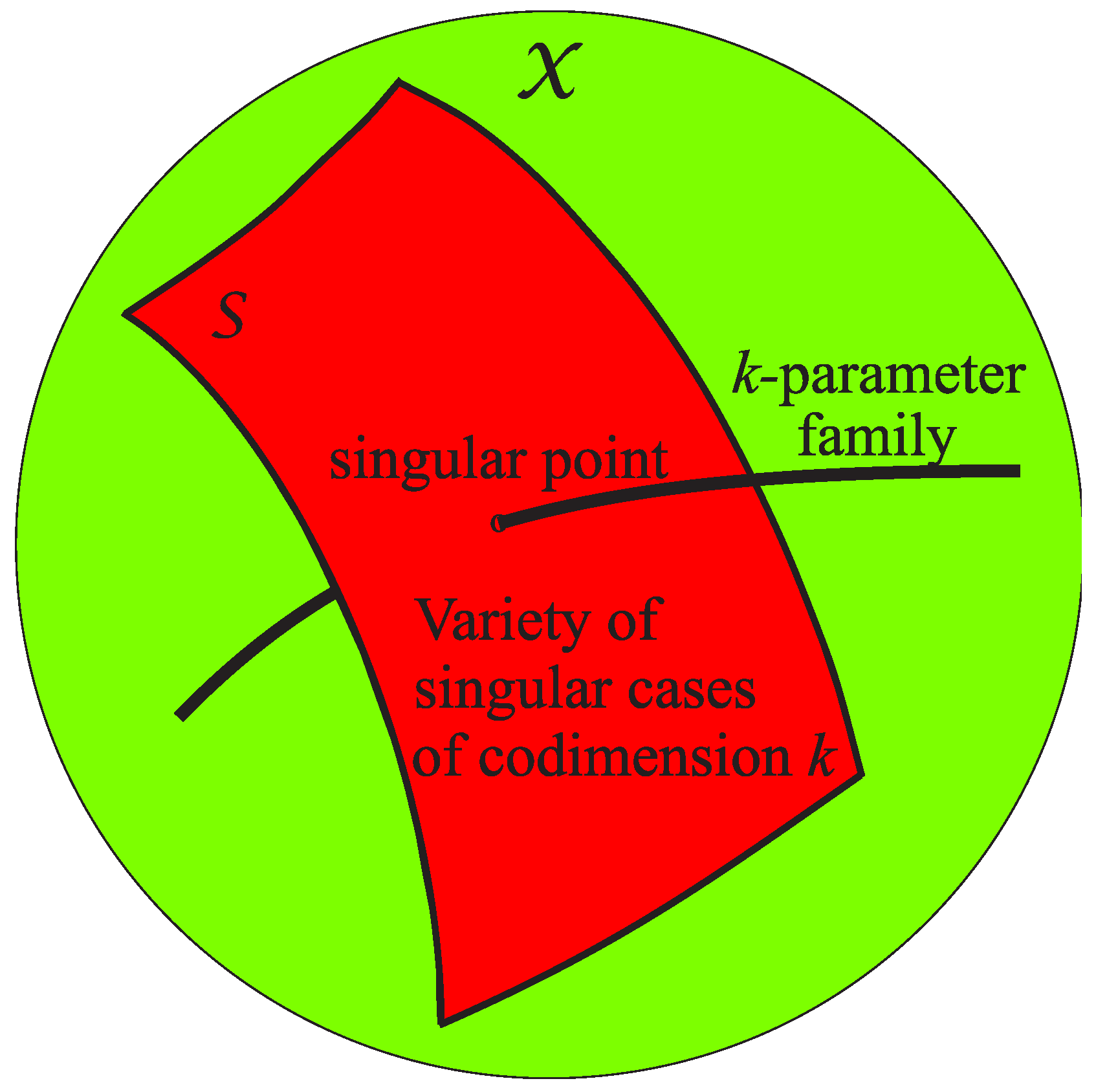
From the point of view of algebraic geometry [25], such a surface represents a variety $\mathcal{S}$ whose dimension typically is strictly smaller than N. We call $\mathcal{S}$ the variety of singular cases. Typically, $\mathcal{S}$ is a closed subset of $\mathcal{X}$, while the set of problems for which $\mathcal{P}$ holds contains an open and dense subset of $\mathcal{X}$.

We say that a property $\mathcal{P}$ is generic relative to $\mathcal{S}$ if $\mathcal{P}\left(x\right)=0$ only for points $x\in \mathcal{S}$. A generic property of a parameter space is a property that holds at “almost all” points of that space. Intuitively, a generic property is one that “almost all” problems satisfy. Equivalently, if the parameters are chosen at random, then $\mathcal{P}=1$ with probability 1.

It should be emphasized that, depending on the problem, the variety of singular cases may have a complex structure. In the special case when the variety has no singular points, it is referred to as manifold.

Since regular problems are generic, they have been studied more thoroughly than the corresponding singular problems. Therefore, the analysis of generic cases is always a primary focus when investigating phenomena and processes described by a given mathematical model. Nevertheless, there are situations in which it becomes necessary to examine non-generic cases. In this context, it is appropriate to quote the words of the great German mathematician Leopold Kronecker, spoken in 1874 [44]: It is customary—especially in algebraic problems—to encounter new difficulties when one moves away from the cases usually regarded as general. As soon as one penetrates beneath the surface of the so-called generality, which excludes all particularities in the true generality encompassing all singularities, one typically first meets the real challenges of investigation, but at the same time also the richness of new perspectives and phenomena contained in its depths.

A property $\mathcal{P}$ is said to be well posed at x if $\mathcal{P}$ holds through some neighborhood of x in $\mathcal{X}$. A problem parametrized by data in $\mathcal{X}$ is said to be well posed at a point $x_0$, if it is solvable for all data points $x_0+\delta$ in some neighborhood of $x_0$. According to the French mathematician Jacques Hadamard [45], a mathematical problem is well posed, if it satisfies the following three conditions:

• a solution exists,
• the solution is unique,
• the solution depends continuously on the data of the problem.

If a problem fails to satisfy at least one of these conditions—namely, if a solution does not exist for some set $\mathcal{S}$ of parameters $x\in \mathcal{S}$, if the solution is not unique, or if the solution does not depend continuously on the parameters—then the problem is called an ill-posed problem.

Ill-posed problems typically form a variety $\mathcal{S}$ within the probelm space, called the set of ill-posed problems.

If the property $\mathcal{P}$ is generic relative to $\mathcal{S}$, then $\mathcal{P}$ is well posed at every point in the complement ${\mathcal{S}}^c$ (where $\mathcal{S}\cup {\mathcal{S}}^c=\mathcal{X}$). Since the dimension of $\mathcal{S}$ is less than the dimension of $\mathcal{X}$, it follows that almost all problems in $\mathcal{X}$ are well posed.

It should be noted, however, that many meaningful and important problems in physics and computational mathematics are not well-posed, that is, they are ill-posed.

Example 10. 

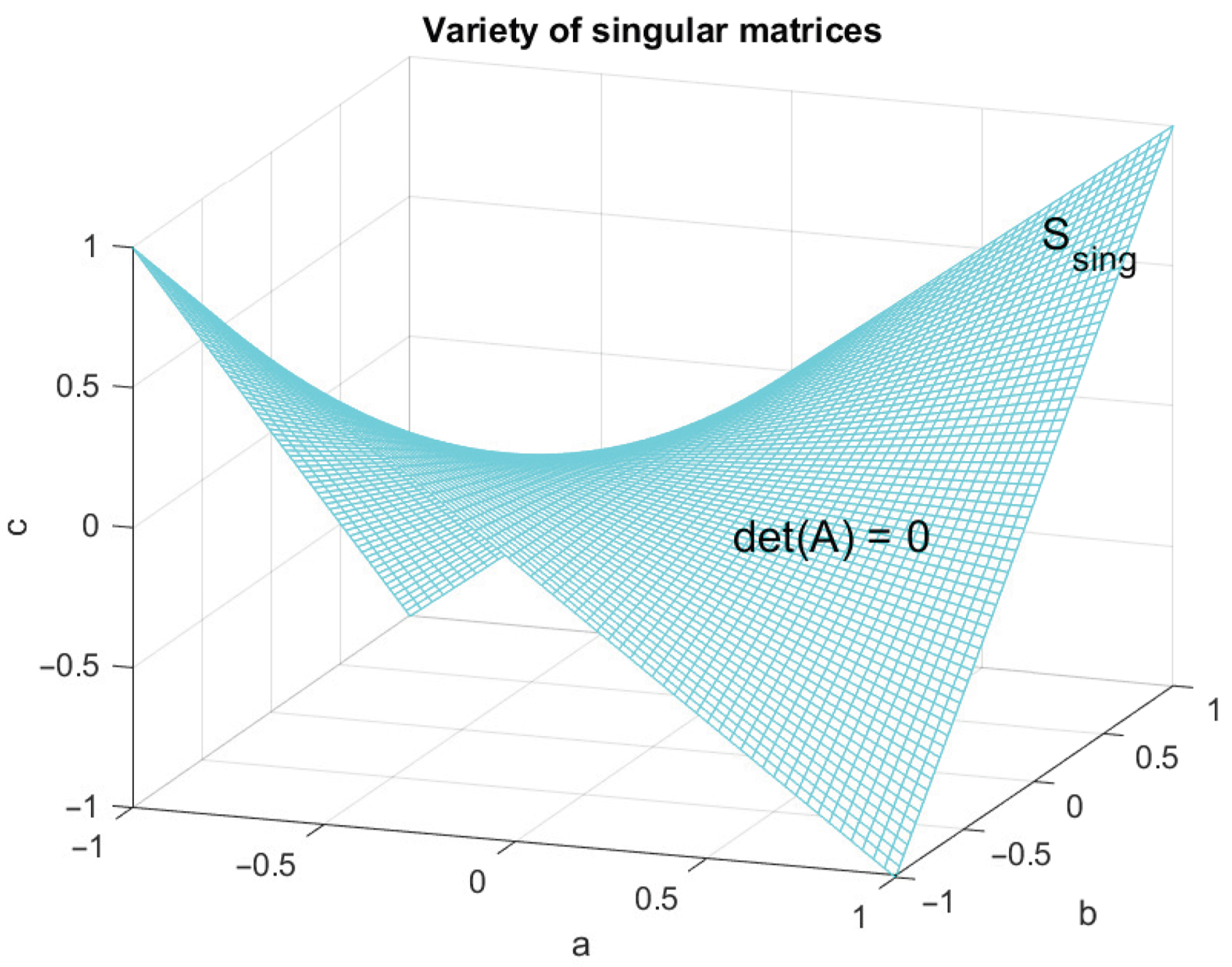
Consider the problem of finding the inverse of a square matrix A of order n. In this case, the property $\mathcal{P}$ is the nonsingularity of the matrix A and the set

$${\mathcal{S}}_{\mathrm{sing}}=\left\{A\in {\mathbb{C}}^{n\times n}:\det \left(A\right)=0\right\}$$

consists of all singular matrices. The set of singular matrices is an algebraic variety, since it can be defined as the zero set of the polynomial $\det \left(A\right)$. Thus, the equation $\det \left(A\right)=0$ describes the variety ${\mathcal{S}}_{\mathrm{sing}}$.

For example, if $n=2,N=3$ and

$$A=\left[\begin{array}{ccc}a& & 1\\ c& & b\end{array}\right],$$

then the variety ${\mathcal{S}}_{\mathrm{sing}}$ is determined by the equality $ab=c$ and represents a hyperbolic paraboloid—a manifold of dimension $2=m\times n-1$ in the three-dimensional parameter space (see Figure 28). All points outside ${\mathcal{S}}_{\mathrm{sing}}$ correspond to nonsingular matrices A, that is matrices for which $\mathcal{P}\left(A\right)=1$.

Example 11. 

Consider the eigenvalue problem for the third-order matrix

$$\begin{array}{c}\hfill \left[\begin{array}{cc}2{p^2}^2+3p^1{p}^2-1& -4{p^2}^2-6p^1{p}^2+2p^1+16p^3+2\dots \\ & -8{p^2}^2-12p^1{p}^2+4p^1+32p^3+4\\ 8{p^1}^2-18p^1{p}^2-4{p^2}^2+2& 8{p^2}^2+12p^1{p}^2-3p^1-24p^3-4\dots \\ & -8{p^1}^2+36p^1{p}^2-6p^1+16{p^2}^2-48p^3-8\\ -4{p^1}^2+9p^1{p}^2+2{p^2}^2-1& -4{p^2}^2-6p^1{p}^2+2p^1+16p^3+2\dots \\ & 4{p^1}^2-18p^1{p}^2+4p^1-8{p^2}^2+32p^3+4\end{array}\right],\end{array}$$

where the entries depend on three parameters $p^1,p^2$, and $p^3$ ($N=3$). In this case, property $\mathcal{P}$ is possessed by matrices with distinct eigenvalues, and the set ${\mathcal{S}}_{\mathrm{mult}}$ consists of all matrices with multiple eigenvalues.

Using the SYMBOLIC TOOLBOX of MATLAB^®, we find that the eigenvalues of A as functions of the parameters are

$$\begin{array}{ccc}\hfill {\lambda }_1& =\hfill & \hfill p^1+8p^3,\\ \hfill {\lambda }_2& =\hfill & \hfill 4{p^1}^2-6p^1{p}^2,\\ \hfill {\lambda }_3& =\hfill & \hfill 2{p^2}^2+3p^1{p}^2-1.\end{array}$$

Assuming that free parameters are $p^1$ and $p^2$, it follows from the expressions for the eigenvalues that, for the given example, two distinct sets of matrices with a double eigenvalue are possible. The first set ${\mathcal{S}}_{{\mathrm{mult}}_1}$ is obtained by equating ${\lambda }_1$ and ${\lambda }_2$:

$${\lambda }_1={\lambda }_2\to p^3={\displaystyle \frac{4{p^1}^2-6p^1{p}^2-p^1}{8}}.$$

The second set, ${\mathcal{S}}_{{\mathrm{mult}}_2}$, is obtained by equating ${\lambda }_1$ and ${\lambda }_3$:

$${\lambda }_1={\lambda }_3\to p^3={\displaystyle \frac{2{p^2}^2+3p^1{p}^2-1-p^1}{8}}.$$

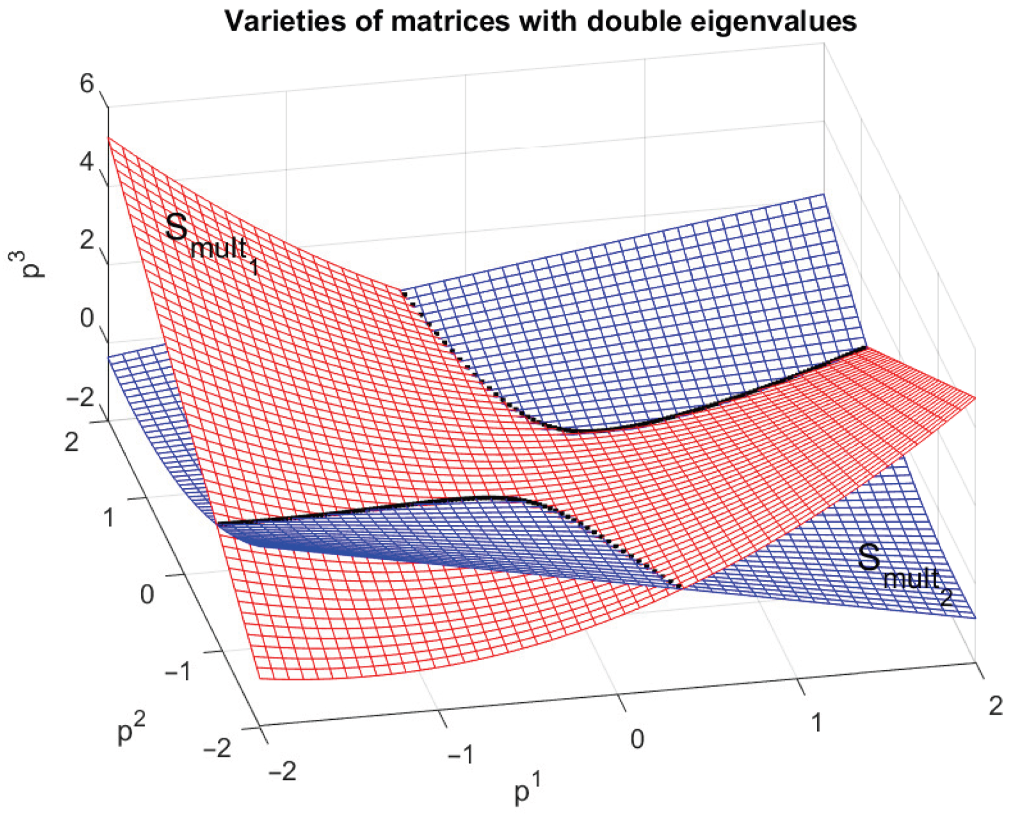
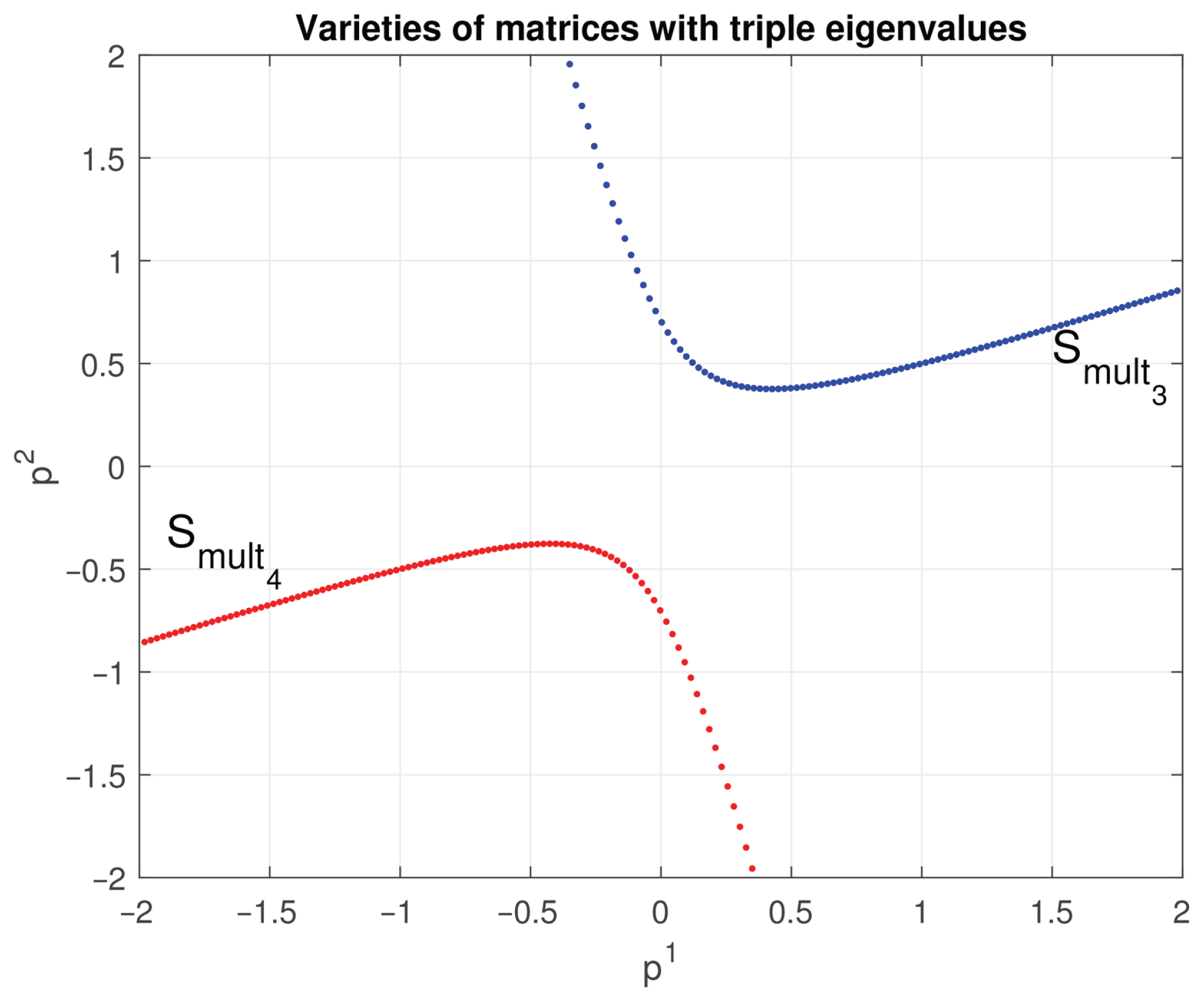
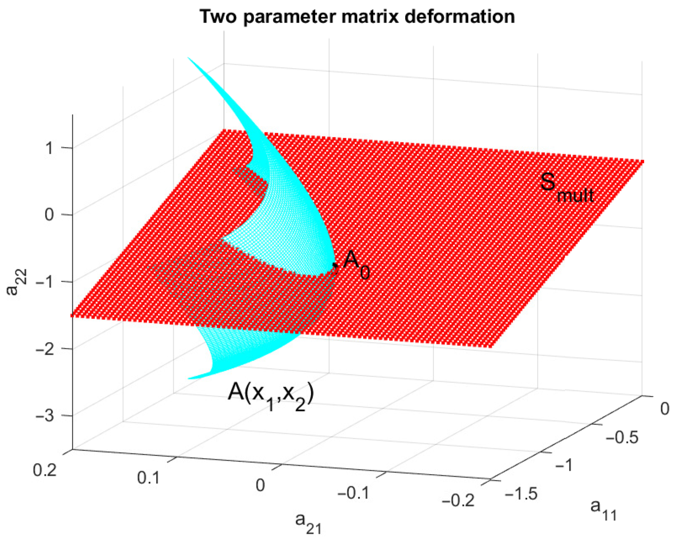
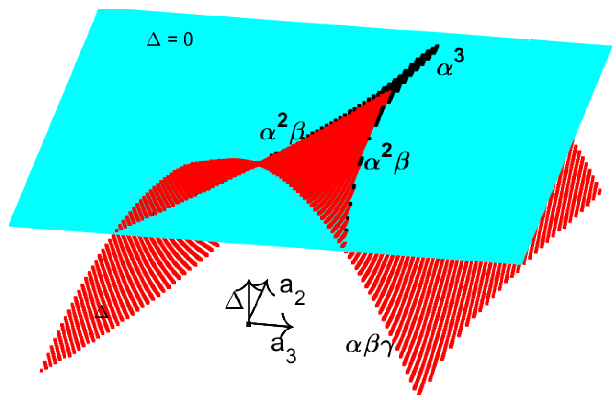
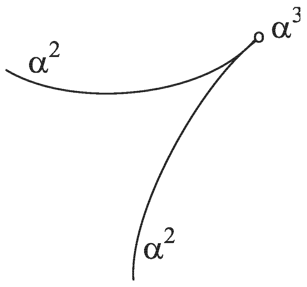
The corresponding surfaces in the three-dimensional parameter space are shown in Figure 29. These varieties of singular cases are hyper-surfaces, i.e., they have codimension one in the three-dimensional parameter space. It should be noted that the double eigenvalues themselves vary with changes in the parameters.

Parameters lying on the intersection of ${\mathcal{S}}_{{\mathrm{mult}}_1}$ and ${\mathcal{S}}_{{\mathrm{mult}}_2}$ satisfy both conditions ${\lambda }_1={\lambda }_2$ and ${\lambda }_1={\lambda }_3$. That is why for these parameter values, the matrix has a triple eigenvalue. By equating the expressions for $p^3$ given above, we find that the parameters corresponding to matrices with a triple eigenvalue satisfy

$$2{p^2}^2+9p^1{p}^2-(4{p^1}^2+1)=0.$$

This condition yields two distinct solutions

$$p_{1,2}^2=-{\displaystyle \frac{9p^1\pm \sqrt{113{p^1}^2+8}}{4}}$$

which define two varieties in the parameter space, ${\mathcal{S}}_{{\mathrm{mult}}_3}$ and ${\mathcal{S}}_{{\mathrm{mult}}_4}$, respectively, of matrices with triple eigenvalues. The same condition can be obtained by directly equating the expressions for ${\lambda }_2$ and ${\lambda }_3$.

These varieties of matrices with triple eigenvalues have codimension two, that is they form curves in the three-dimensional space. A two-dimensional projection of these curves is shown in Figure 30.

Since there are two varieties of matrices with double or triple eigenvalues, it is natural to define ${\mathcal{S}}_{{\mathrm{mult}}_1}\cup {\mathcal{S}}_{{\mathrm{mult}}_2}$ as the set of matrices with double eigenvalues, and  ${\mathcal{S}}_{{\mathrm{mult}}_3}\cup {\mathcal{S}}_{{\mathrm{mult}}_4}$ as the set of matrices with triple eigenvalues.

Matrices with parameters lying outside these sets have distinct (simple) eigenvalues.

Since the set of regular problems is dense and the set of singular problems has measure zero in finite-dimensional spaces, numerical algorithms typically perform reliably, but may fail catastrophically near singular strata.

3.3. Conditioning of Computational Problems

To obtain an accurate solution of a computational problem, it is not sufficient for the problem to be well posed. If the problem lies close in the norm of the problem’s data space to the set $\mathcal{S}$ of ill-posed problems, then it may be highly sensitive to perturbations, and the discrepancy between the computed and the exact solutions can be very large.

The sensitivity of a given mathematical problem describes how its solution varies in the vicinity of a nominal solution. This important property of mathematical problems is the subject of perturbation theory, which is widely used in science and engineering.

A simplified quantitative characterization of sensitivity can be obtained by using the notion of conditioning.

Conditioning is a property of a computational problem that characterizes the sensitivity of its solution to small changes (or perturbations) in the data. A problem is said to be well conditioned, if small perturbations in the data lead to small changes in the solution. Conversely, if small changes in the data may result in large changes in the solution, the problem is called ill conditioned.

It should be emphasized that the conditioning is an intrinsic property of the problem itself. It does not depend on the numerical precision used to solve the problem, nor does it depend on the particular numerical method implemented.

The theory of conditioning is developed in [46,47]. Various kinds of condition numbers are discussed in [48,49], while the computing of condition estimates is addressed in [50], (Ch. 15, [51]), [52,53]. The conditioning of differentiable maps between smooth matrix manifolds is studied in [54].

3.4. Condition Numbers

Consider the computational problem $y=f\left(x\right)$, where f maps the input data x to the output y. The problem is said to be well conditioned if $f\left(x\right)$ is relatively insensitive to small perturbations $\delta x$ in x, that is, $f\left(x\right)$ remains close to $f\left(x_0\right)$ when $x=x_0+\delta x$ is near $x_0$. The precise meaning of “insensitive”, “small” and “close” depends on the specific context of the problem. Conversely, if small changes in x produce large variations in f, the problem is ill conditioned.

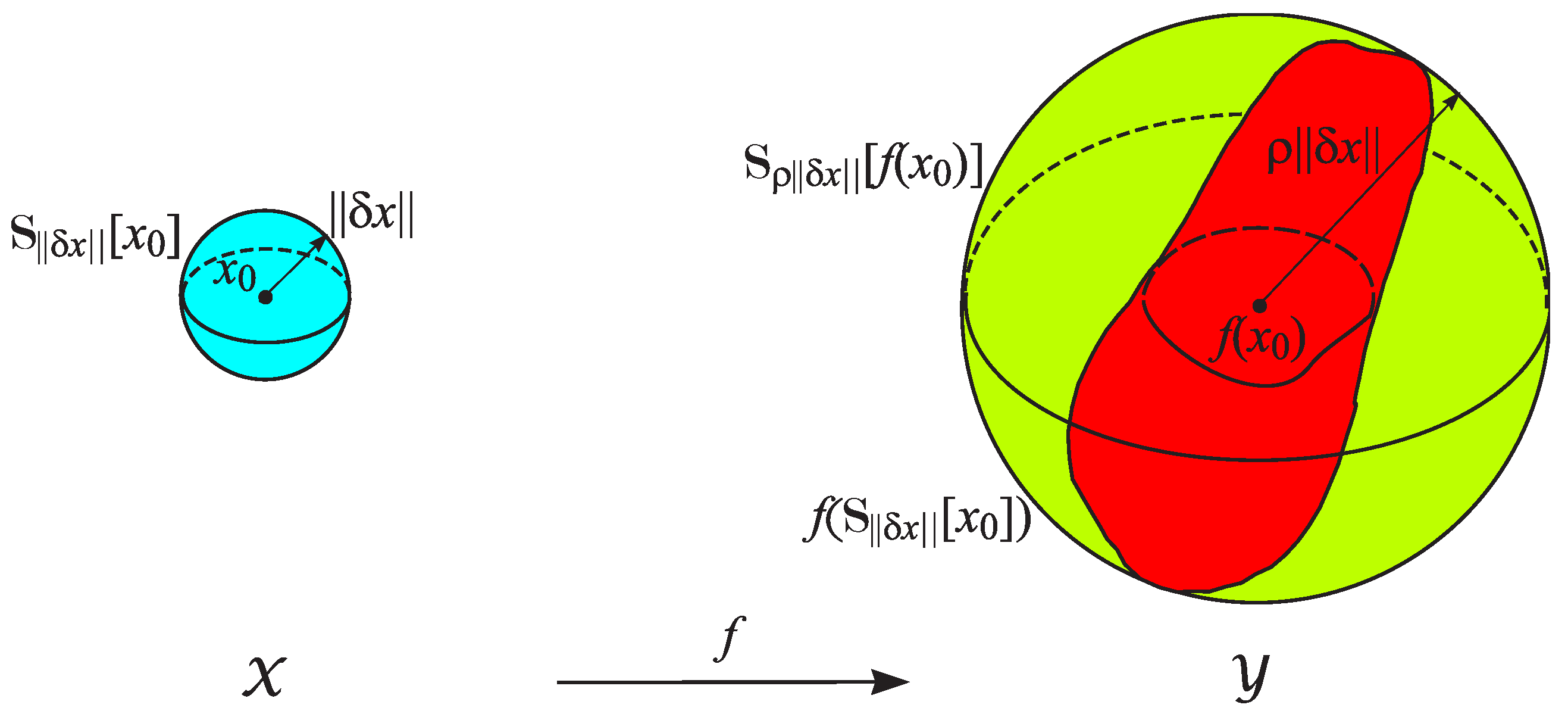
The conditioning of a computational problem can be formally characterized as illustrated in Figure 31 where $\parallel .\parallel$ denotes the Euclidean vector norms in $\mathcal{X}$ and $\mathcal{Y}$, respectively.

Definition 14 

(Absolute condition number). The absolute $\delta x$-condition number of the mapping $f:\mathcal{X}\to \mathcal{Y}$ at the point $x_0\in \mathcal{X}$ is defined as

$${\kappa }_{\delta x}^{abs}(f,x_0)=\inf \{\rho :f[{\mathbb{S}}_x(x_0,\parallel \delta x\parallel \left)\right]\subset {\mathbb{S}}_y(f\left(x_0\right),\rho \parallel \delta x\parallel \left)\right\}.$$

(3)

According to this definition, the condition number ${\kappa }_{\delta x}^{abs}$ is the smallest number $\rho$ such that the image $f[{\mathbb{S}}_x(x_0,\parallel \delta x\parallel \left)\right]$ of the sphere ${\mathbb{S}}_x(x_0,\parallel \delta x\parallel )$ lies entirely within the sphere ${\mathbb{S}}_y(f\left(x_0\right),\rho \parallel \delta x\parallel )$ of a radius $\rho \parallel \delta x\parallel$.

Defined in this way, the condition number can be interpreted as a Lipschitz constant for the mapping f, i.e., it is the smallest number M for which

$$\parallel f(x_0+\delta x)-f\left(x_0\right)\parallel \le M\parallel x-x_0\parallel$$

holds for all points on the boundary of $\mathbb{S}(x_0,\parallel \delta x\parallel )$. Note that this gives a first-order estimate of sensitivity.

As illustrated in Figure 31, the condition number $\kappa$ provides a quantitative measure of how perturbations in the data are transmitted to the solution space $\mathcal{Y}$. If $\kappa$ is relatively small, the problem is well conditioned; if $\kappa$ is large, the problem is ill conditioned.

Definition 15 

(Relative condition number). The relative $\delta x$-condition number of the mapping $f:\mathcal{X}\to \mathcal{Y}$ at the point $x_0\in \mathcal{X}$ is defined as

$${\kappa }_{\delta x}^{rel}(f,x_0)=\inf \{\rho :f[{\mathbb{S}}_x^r(x_0,\parallel \delta x\parallel \left)\right]\subset {\mathbb{S}}_y^r(f\left(x_0\right),\rho \parallel \delta x\parallel \left)\right\}.$$

(4)

In many practical applications, it is common to consider the condition number if the perturbation in the limit of infinitesimally small perturbations $\parallel \delta x\parallel$. Although this represents a theoretical approximation, it is widely used in perturbation analysis because it is easier to compute.

Definition 16  

(Asymptotic condition number). The asymptotic absolute and asymptotic relative condition number of $f:\mathcal{X}\to \mathcal{Y}$ are defined, respectively, as 

$$\begin{array}{ccc}\hfill \left(i\right){\kappa }^{abs}(f,x_0)& =& {\lim }_{\parallel \delta x\parallel \to 0}{\kappa }_{\delta x}^{abs}(f,x_0),\hfill \end{array}$$

(5)

$$\begin{array}{ccc}\hfill \left(ii\right){\kappa }^{rel}(f,x_0)& =& {\lim }_{\parallel \delta x\parallel \to 0}{\kappa }_{\delta x}^{rel}(f,x_0).\hfill \end{array}$$

(6)

If the Jacobian matrix $D_{x_0}f$ of the mapping f exists, then the asymptotic absolute and relative condition numbers are given by

$$\begin{array}{ccc}\hfill \left(i\right){\kappa }^{abs}(f,x_0)& =& \parallel D_{x_0}f\parallel ,\hfill \end{array}$$

(7)

$$\begin{array}{ccc}\hfill \left(ii\right){\kappa }^{rel}(f,x_0)& =& {\displaystyle \frac{\parallel D_{x_0}f\parallel \parallel x_0\parallel }{\parallel f\left(x_0\right)\parallel }},\hfill \end{array}$$

(8)

where $\parallel D_{x_0}f\parallel$ denotes the operator (subordinate norm) of the derivative $D_{x_0}f$ in $\mathcal{Y}$.

The asymptotic condition number is usually referred to as the condition number of the problem. Note that this condition number does not exist for all mappings f.

The asymptotic absolute and relative condition numbers can be expressed as

$${\kappa }^{abs}(f,x_0):=\underset{\parallel \delta x\parallel \to 0}{lim}sup{\displaystyle \frac{\parallel f(x_0+\delta x)-f\left(x_0\right)\parallel }{\parallel \delta x\parallel }}=\parallel D_{x_0}f\parallel ,$$

(9)

$$\begin{array}{ccc}\hfill {\kappa }^{rel}(f,x_0)& :=& \underset{\parallel \delta x\parallel \to 0}{lim}sup{\displaystyle \frac{\parallel f(x_0+\delta x)-f\left(x_0\right)\parallel /\parallel f\left(x_0\right)\parallel }{\parallel \delta x\parallel /\parallel x_0\parallel }}\hfill \\ & =& {\displaystyle \frac{\parallel D_{x_0}f\parallel \parallel x_0\parallel }{\parallel f\left(x_0\right)\parallel }}\hfill \end{array}$$

(10)

which coincides with the expressions in (7) and (8).

From this definition, it follows that

$$\begin{array}{ccc}\hfill {\displaystyle \frac{\parallel f(x_0+\delta x)-f\left(x_0\right)\parallel }{\parallel f\left(x_0\right)\parallel }}& \le & {\kappa }^{rel}(f,x_0){\displaystyle \frac{\parallel \delta x\parallel }{\parallel x_0\parallel }}+o\left(\delta x\right),\hfill \end{array}$$

(11)

where $h=o\left(\right|\delta x\left|\right)$ means $\left|h\right|/\left|\delta x\right|\to 0$ as $\left|\delta x\right|\to 0$.

Equation (11) shows that the relative change in the result can be approximated by the product of the relative condition number ${\kappa }^{rel}(f,x_0)$ and the relative perturbation $\parallel \delta x\parallel /\parallel x_0\parallel$ in the data. The ratio $\parallel \delta x\parallel /\parallel x_0\parallel$ is called backward error since the change in the solution is represented as an equivalent perturbation in the input data equivalent to the observed change in the solution. The backward error measures how much you would need to perturb the input to get the computed output exactly. Computational methods for which the backward error is small are called numerically stable.

Consequently, the quantity

$${\kappa }^{rel}(f,x_0){\displaystyle \frac{\parallel \delta x\parallel }{\parallel x_0\parallel }}$$

provides an estimate of the relative forward error in the solution, given the relative backward error. If the condition number is large, even small perturbations in the input may produce a large forward error, highlighting the difficulty of the computational problem.

It should be noted that even well-conditioned problems may have specific perturbations for which the sensitivity estimate overstates the true change in the solution. When the sensitivity estimate consistently produces overly pessimistic bounds, it is called a conservative estimate.

3.5. Conditioning of Basic Matrix Problems

In this section we present two case studies that illustrate the concept of conditioning in matrix computations.

3.5.1. Conditioning of a Linear System of Equations

Consider the linear system

$$Ay=x,$$

where $A\in {\mathbb{C}}^{n\times n}$ is nonsingular and $y=A^{-1}x,x\ne 0$. Solving the system corresponds to applying the linear operator $x\to A^{-1}x$.

The entries of A serve as parameters, and the set of singular matrices forms a variety ${\mathcal{S}}_{\mathrm{sing}}$, representing ill-posed problems. Small perturbations $\delta A$ may therefore lead to large changes in the solution.

Assuming that A is perturbed to $A+\delta A$, the perturbed solution satisfies

$$y+\delta y={(A+\delta A)}^{-1}x.$$

(12)

The matrix $A+\delta A$ remains nonsingular if

$$\parallel A^{-1}{\delta A\parallel }_2<1.$$

(13)

Under this condition, standard perturbation theory (Ch. 3, [55]), (Sect. 2.6, [56]), (Sect. 1.2, [57]) yields the relative error bound

$${\displaystyle \frac{{\parallel \delta y\parallel }_2}{{\parallel y\parallel }_2}}\le {\displaystyle \frac{{\parallel A\parallel }_2{\parallel A^{-1}\parallel }_2}{1-\parallel A^{-1}{\delta A\parallel }_2}}{\displaystyle \frac{{\parallel \delta A\parallel }_2}{{\parallel A\parallel }_2}}.$$

(14)

According to Definition 15, the product

$${\kappa }^{rel}={\parallel A\parallel }_2{\parallel A^{-1}\parallel }_2$$

represents the relative condition number of the linear system. It satisfies ${\kappa }^{rel}\ge 1$ and is invariant under scalar multiplication of A. For sufficiently small perturbations, the bound simplifies asymptotically to

$${\displaystyle \frac{{\parallel \delta y\parallel }_2}{{\parallel y\parallel }_2}}\le {\kappa }^{rel}{\displaystyle \frac{{\parallel \delta A\parallel }_2}{{\parallel A\parallel }_2}}.$$

(15)

If ${\kappa }^{rel}$ is small, the system is well conditioned; if large, it is ill conditioned. When ${\kappa }^{rel}\approx 1/\mathrm{u}$, where $\mathrm{u}$ is the unit roundoff, the matrix is considered singular to working precision, and the computed solution may lose all significant digits.

Following standard notation, the condition number is denoted by

$${\mathrm{cond}}_2\left(A\right)={\parallel A\parallel }_2{\parallel A^{-1}\parallel }_2.$$

The value of the condition number depends on the chosen norm. In particular, using the singular value decomposition $A=U\mathsf{\Sigma }{V}^T$,

$${\mathrm{cond}}_2\left(A\right)={\displaystyle \frac{{\sigma }_{max}}{{\sigma }_{min}}},$$

where ${\sigma }_{max}$ and ${\sigma }_{min}$ are the largest and smallest singular values of A. The 2-norm or the Frobenius norm condition numbers are invariant under unitary (orthogonal) transformations.

Example 12. 

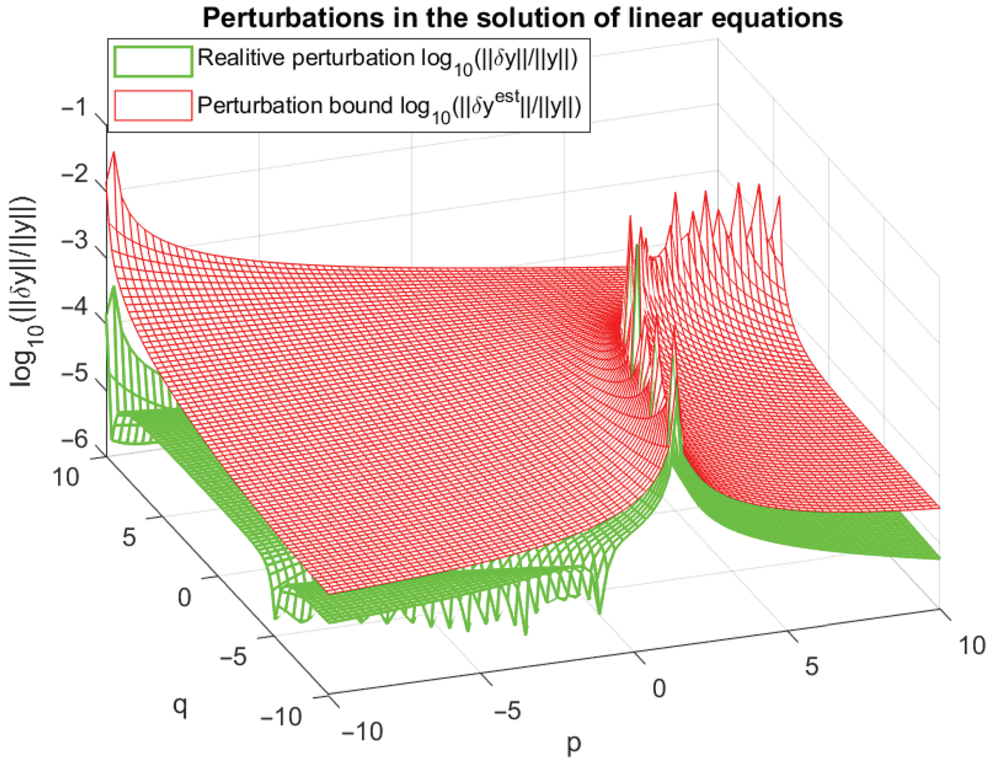
Consider the linear system $Ay=x$, where

$$A=\left[\begin{array}{cccccc}\hfill -6& \hfill 2& \hfill 5& \hfill -3& \hfill p& \hfill 1\\ \hfill 3& \hfill -1& \hfill -4& \hfill 3& \hfill -8& \hfill -2\\ \hfill q& \hfill 7& \hfill -2& \hfill -5& \hfill 4& \hfill -3\\ \hfill -2& \hfill -8& \hfill 9& \hfill 4& \hfill -5& \hfill 7\\ \hfill 9& \hfill 0& \hfill 6& \hfill -1& \hfill -7& \hfill 3\\ \hfill 5& \hfill 8& \hfill -3& \hfill -6& \hfill 2& \hfill 4\end{array}\right],x=\left[\begin{array}{c}\hfill -2\\ \hfill 7\\ \hfill -5\\ \hfill -3\\ \hfill 9\\ \hfill 1\end{array}\right]$$

and $p\in [-10,10],q\in [-10,10]$ are variable parameters. Assume that the matrix A is subject to the perturbation

$$\delta A={10}^{-6}\left[\begin{array}{cccccc}\hfill 2& \hfill 5& \hfill 8& \hfill 9& \hfill 3& \hfill 4\\ \hfill 6& \hfill -4& \hfill -7& \hfill -2& \hfill -5& \hfill 1\\ \hfill -3& \hfill 1& \hfill 0& \hfill 4& \hfill 6& \hfill -2\\ \hfill -4& \hfill 1& \hfill 2& \hfill -9& \hfill -8& \hfill 5\\ \hfill 8& \hfill -5& \hfill 3& \hfill 2& \hfill 0& \hfill 1\\ \hfill -7& \hfill 9& \hfill -2& \hfill -3& \hfill 5& \hfill 0\end{array}\right].$$

In Figure 32, we display the relative perturbation

$${\displaystyle \frac{{\parallel \delta y\parallel }_2}{{\parallel y\parallel }_2}}$$

in the solution caused by the perturbation $\delta A$, as a function of the parameters p and q. This is shown together with the corresponding relative perturbation estimate

$${\displaystyle \frac{\parallel \delta y^{est}{\parallel }_2}{{\parallel y\parallel }_2}}={\displaystyle \frac{{\mathrm{cond}}_2\left(A\right)\frac{{\parallel \delta A\parallel }_2}{{\parallel A\parallel }_2}}{1-{\mathrm{cond}}_2\left(A\right)\frac{{\parallel \delta A\parallel }_2}{{\parallel A\parallel }_2}}}.$$

The peak values in the Figure represent ill conditioned matrices. The maximum condition number of the perturbed matrices is ${\mathrm{cond}}_2\left(A\right)=3.21\times {10}^5$ which leads to maximum relative perturbations of size $0.1$. Note that ${\mathrm{cond}}_2\left(A\right)$ is typically computed via the singular value decomposition of A.

3.5.2. Conditioning of the Eigenvalue Problem

We consider, in a simplified setting, the problem of sensitivity of the eigenvalues of a matrix. This problem is characterized by fundamentally different properties in the regular case, when the eigenvalues are distinct, and in the singular case, when the eigenvalues are multiple and possess nonlinear elementary divisors.

Let us first examine the asymptotic sensitivity of the eigenvalue problem in the regular case. In this case, the eigenvalue problem is well posed, since the variations in the eigenvalues depend linearly on the perturbations in the entries of the matrix.

Let $A\in {\mathbb{C}}^{n\times n}$ be a given square matrix. If A has a simple eigenvalue $\lambda$, with corresponding right eigenvector $x\in {\mathbb{C}}^n$ and left eigenvector $y\in {\mathbb{C}}^n$, then

$$Ax=\lambda x\mathrm{and}{y}^{H}A=\lambda y^H,$$

where $y^H$ denotes the conjugate transpose of y. Since $\lambda$ is a simple eigenvalue, it follows that

$$y^{H}x=\langle x,y\rangle \ne 0.$$

For every sufficiently small perturbation $\delta A\in {\mathbb{C}}^{n\times n}$, there exists a unique eigenvalue $\lambda +\delta \lambda$ of $A+\delta A$, that is close to $\lambda$. Therefore, we have

$$(A+\delta A)(x+\delta x)=(\lambda +\delta \lambda )(x+\delta x),$$

which implies that, up to terms of second order,

$$\delta Ax+A\delta x\approx \delta \lambda x+\lambda \delta x.$$

Multiplying from the left by $y^H$, we obtain

$$\delta \lambda ={\displaystyle \frac{1}{\langle x,y\rangle }}{y}^H\delta Ax+{o(\parallel \delta A\parallel }_2).$$

Moreover,

$$\underset{{\parallel \delta A\parallel }_2\le 1}{max}|y^H{\delta Ax|=\parallel x\parallel }_2{\parallel y\parallel }_2.$$

Therefore, absolute condition number of the matrix A with respect to the regular eigenvalue problem can be defined as

$${\kappa }_{\lambda }^{abs}\left(A\right):={\displaystyle \frac{{\parallel x\parallel }_2{\parallel y\parallel }_2}{\langle x,y\rangle }}.$$

We have that

$${\kappa }_{\lambda }^{abs}\left(A\right)={\parallel P\parallel }_2,$$

(16)

where

$$P={\displaystyle \frac{x{y}^H}{y^{H}x}}$$

is the spectral projector onto the invariant subspace generated by x. If the right and left eigenvector are normalized so that $y^{H}x=1$, then

$${\kappa }_{\lambda }^{abs}\left(A\right):={\parallel x\parallel }_2{\parallel y\parallel }_2.$$

The condition number is homogeneous, since multiplying A by a scalar does not change ${\kappa }_{\lambda }^{abs}\left(A\right)$. It is also invariant under unitary (or orthogonal) transformations.

If ${\kappa }_{\lambda }^{abs}\left(A\right)$ is large, then $\lambda$ is poorly conditioned. Poorly conditioned eigenvalues are computed with large errors as a consequence of their high sensitivity to perturbations in the matrix. As the separation between eigenvalues decreases, their sensitivity increases, and in the limiting case of defective eigenvalues, their condition numbers become infinitely large. In such cases, the linear estimate

$$\left|\delta \lambda \right|\le {\kappa }_{\lambda }^{abs}\left(A\right){\parallel \delta A\parallel }_2,$$

(17)

is no longer valid, and the eigenvalue problem becomes ill-posed. In this case, it is justified to set ${\kappa }_{\lambda }^{abs}\left(A\right):=\infty$, where $\lambda$ is a multiple eigenvalue of A.

We note that the eigenvalue sensitivity estimates provided by the linear algebra package LAPACK [58] and the software system MATLAB^® [2] yield meaningful results only for well-posed problems, specifically when the matrices have simple eigenvalues, i.e., eigenvalues to which correspond linearly independent eigenvectors.

Example 13. 

Consider the upper triangular matrix

$$A=\left[\begin{array}{ccc}{\lambda }_1& & 1\\ 0& & {\lambda }_1+\epsilon \end{array}\right],\epsilon \ne 0.$$

The matrix A has two simple eigenvalues ${\lambda }_1$ and ${\lambda }_2={\lambda }_1+\epsilon$. The corresponding spectral projectors are

$$P_{{\lambda }_1}=\left[\begin{array}{ccc}1& & -1/\epsilon \\ 0& & 0\end{array}\right]and{P}_{{\lambda }_2}=\left[\begin{array}{ccc}0& & 1/\epsilon \\ 0& & 1\end{array}\right].$$

Both eigenvalues have the same absolute condition number given by

$${\kappa }_{\lambda }^{abs}\left(A\right)={\displaystyle \frac{\sqrt{1+{\left|\epsilon \right|}^2}}{\left|\epsilon \right|}}.$$

As $\epsilon \to 0$, the condition number tends to infinity, since the two eigenvalues of A coalesce (${\lambda }_1={\lambda }_2=\lambda$) and the eigenvalue problem becomes ill-posed.

Since the eigenvalue condition number becomes infinite when $\lambda$ is a multiple eigenvalue, the variety of singular cases for the eigenvalue problem consists of all matrices with multiple eigenvalues. This variety forms a hypersurface in the space of $n\times n$ matrices, i.e., it has dimension $N-1$, where $N=n^2$.

For matrices with multiple eigenvalues, small perturbations of the entries can cause large changes in the eigenvalues. Such matrices are characterized by eigenvalues that appear in nonlinear elementary divisors.

Following [59,60], we now examine the sensitivity of the eigenvalue problem in the singular case.

Let the Jordan form of A corresponding to the multiple eigenvalue $\lambda$ be arranged in q groups of Jordan blocks, each group consisting of blocks of the same size:

$$J=\mathrm{diag}\left(\underset{r_1}{\underbrace{{\mathsf{\Gamma }}_1^1,\dots ,{\mathsf{\Gamma }}_1^{r_1}}},\dots ,\underset{r_j}{\underbrace{{\mathsf{\Gamma }}_j^1,\dots ,{\mathsf{\Gamma }}_j^{r_j}}},\dots ,\underset{r_q}{\underbrace{{\mathsf{\Gamma }}_q^1,\dots ,{\mathsf{\Gamma }}_q^{r_q}}}\right),$$

where, for $j=1,\dots ,q$,

$${\mathsf{\Gamma }}_j^1=\dots ={\mathsf{\Gamma }}_j^{r_j}=\left[\begin{array}{ccccc}\lambda & 1& & & \\ & \dot{}& \dot{}& & \\ & & \dot{}& \dot{}& \\ & & & 1& \dot{}\\ & & & & \lambda \end{array}\right]$$

is a Jordan block of dimension $n_j$, repeated $r_j$ times, and

$$n_1\ge \dots \ge n_j\ge \dots \ge n_q.$$

The quantities $r_1$ (the number of Jordan blocks of maximum size $n_1$) and q (the number of groups of Jordan blocks) play an important role in the eigenvalue sensitivity.

The eigenvalue $\lambda$ is semisimple (i.e., nondefective, participating in $r_1$ Jordan blocks of size 1) if $q=n_1=1$, and nonderogatory (participating in only one Jordan block) if $q=r_1=1$.

It follows that the algebraic and geometric multiplicities of $\lambda$, are, respectively,

$$m=\sum _{j=1}^q{r}_j{n}_j\mathrm{and}g=\sum _{j=1}^q{r}_j.$$

Denote by $x_1^k$ the right eigenvector and by $y_1^k$ the left eigenvector of A associated with ${\mathsf{\Gamma }}_1^k,k=1,\dots ,r_1$. With these eigenvectors we construct the matrices

$$X_1=\left[x_1^1,\dots ,x_1^{r_1}\right],Y_1=\left[y_1^1,\dots ,y_1^{r_1}\right],$$

corresponding to the Jordan blocks of maximum size $n_1$. Note that the $r_1$ columns of $X_1$ and $Y_1$ are linearly independent right and left eigenvectors, respectively, each associated with a separate Jordan chain of maximal length $n_1$.

Assume that the matrix A is perturbed to $A+\epsilon B$, where $\epsilon$ is small. It is shown in [59,60] that the eigenvalues $\tilde{\lambda }$ of $A+\epsilon B$ converging to $\lambda$ as $\epsilon \to 0$ satisfy

$$|\tilde{\lambda }{-\lambda |\le c\left(\alpha \epsilon \right)}^{1/n_1},$$

(18)

for all sufficiently small positive $\epsilon$, where $\alpha =\parallel X_1{Y}_1^H{\parallel }_2$ and $c>1$.

The bound (18) shows that the sensitivity of a multiple eigenvalue depends on ${\epsilon }^{1/n_1}$, where $n_1$ is the size of the largest Jordan block associated with $\lambda$.

For a simple $\lambda$, $n_1=r_1=1$, and $\alpha ={\parallel x\parallel }_2{\parallel y\parallel }_2$, whith normalization $y^{H}x=1$. In this case, the bound (18) coincides with the bound (17) valid for a simple eigenvalue. It is important to note that the bound (18) remains finite, while the linear bound (17) becomes infinite in this case.

In the case where $\lambda$ is semisimple, that is $q=n_1=1$, Equation (18) reduces to

$$|\tilde{\lambda }-\lambda |\le c\alpha \epsilon ,$$

which shows that the eigenvalue bound depends linearly on the perturbation magnitude.

If $\lambda$ is nonderogatory (i.e., there is only one Jordan block corresponding to $\lambda$), then $q=r_1=1$. Substituting into (18), we again obtain $\alpha ={\parallel x\parallel }_2{\parallel y\parallel }_2$, where x and y are the corresponding right and left eigenvectors associated with ${\mathsf{\Gamma }}_1^1$. In this case, expression (18) yields the maximum possible value of ${\epsilon }^{1/n_1}$, since $n_1$ coincides with the algebraic multiplicity m of $\lambda$.

The following example illustrates how the dimension of the Jordan block associated with a multiple eigenvalue affects its sensitivity.

Example 14. 

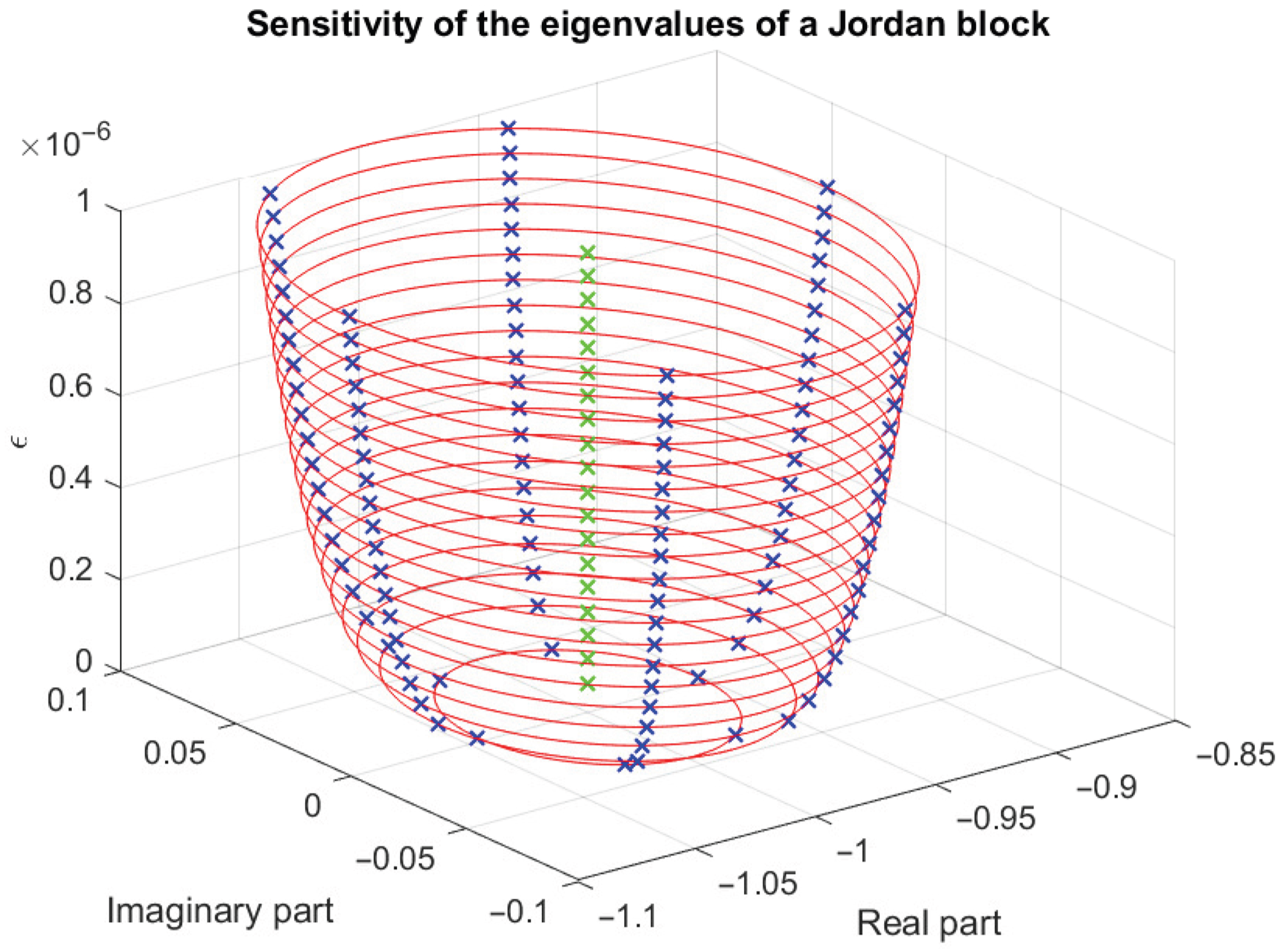
Consider a Jordan block $J_n\left(\lambda \right)$ of nth order with eigenvalue λ. If the zero entry in position $(n,1)$ is replaced by a small number $\epsilon >0$, the characteristic equation of the perturbed block becomes

$${(\lambda -\tilde{\lambda })}^n-{(-1)}^n\epsilon =0$$

and the multiple eigenvalue λ is split into n distinct eigenvalues

$${\tilde{\lambda }}_k=\lambda +{\epsilon }^{1/n}(cos(2k\pi /n)+j_{o}sin(2k\pi /n)),k=0,1,\dots ,n-1.$$

In the given case $n_1=6,r_1=1$ and $J_n\left(\lambda \right)$ has one right eigenvector $x={\left[100000\right]}^T$ and one left eigenvector $y={\left[00001\right]}^T$ so that $\alpha =\parallel x\parallel \parallel y\parallel =1$. The perturbed eigenvalues satisfy

$$|{\tilde{\lambda }}_k-\lambda |={\epsilon }^{1/n},$$

as predicted by (18).

For instance, consider

$$J_6(-1)=\left[\begin{array}{cccccc}\hfill -1& \hfill 1& \hfill 0& \hfill 0& \hfill 0& \hfill 0\\ \hfill 0& \hfill -1& \hfill 1& \hfill 0& \hfill 0& \hfill 0\\ \hfill 0& \hfill 0& \hfill -1& \hfill 1& \hfill 0& \hfill 0\\ \hfill 0& \hfill 0& \hfill 0& \hfill -1& \hfill 1& \hfill 0\\ \hfill 0& \hfill 0& \hfill 0& \hfill 0& \hfill -1& \hfill 1\\ \hfill 0& \hfill 0& \hfill 0& \hfill 0& \hfill 0& \hfill -1\end{array}\right],$$

with $n=6$ and $\lambda =-1$. For $\epsilon ={10}^{-6}$, the perturbed eigenvalues are

$$\begin{array}{c}-0.900000000000000,\hfill \\ -0.950000000000000+j_{o}0.086602540378444,\hfill \\ -0.950000000000000-j_{o}0.086602540378444,\hfill \\ -1.050000000000000+j_{o}0.086602540378444,\hfill \\ -1.050000000000000-j_{o}0.086602540378444,\hfill \\ -1.100000000000000.\hfill \end{array}$$

The perturbations in the eigenvalues are exactly ${\epsilon }^{1/6}=0.1$, which is ${10}^5$ larger than the original perturbation $\epsilon ={10}^{-6}$.

In Figure 33, we show the eigenvalue perturbations of $J_6(-1)$ for 20 equally spaced values of ε between ${10}^{-8}$ (bottom circle) and ${10}^{-6}$ (top circle). Note that the number of the eigenvalue loci is equal to the size of the Jordan block.

Thus, a perturbation of size ε can induce changes of order ${\epsilon }^{1/n}$ in the eigenvalues, which can be large even for moderate n. Since the trace of the matrix is unchanged, the mean of the eigenvalues ${\sum }_1^n{\lambda }_i/n$ remains λ.

In this example, the eigenvalues are highly sensitive to perturbations because the matrix is completely defective. In contrast, eigenvalues corresponding to linear elementary divisors generally exhibit low sensitivity. This illustrates that any meaningful analysis of eigenvalue sensitivity must, either explicitly or implicitly, take the Jordan structure of the matrix into account. As we will see in Section 5, when the defective eigenvalue is associated with a single Jordan block of order n, the corresponding variety of matrices with multiple eigenvalues has the higher possible codimension, equal to $n-1$. This demonstrates that increasing codimension is accompanied by a deterioration in eigenvalue conditioning.

More generally, ill-conditioning in a matrix problem arises when the problem lies close to a variety of high codimension.

A large body of results on the sensitivity of matrix eigenvalues can be found in the books [56,61,62,63,64,65]. The book by Stewart and Sun [66] provides a detailed presentation of various methods for perturbation analysis of eigenvalue and eigenvector problems. Comprehensive surveys of such methods are also given in [67,68]. Several important results on eigenvalue sensitivity have been published in [69,70,71,72,73,74,75,76], among others. The eigenvalue problem for matrices with very ill-conditioned eigenvalues is studied in [77,78]. Theoretical and practical aspects of eigenvalue conditioning analysis are addressed in [79,80,81,82,83,84].

3.6. Distance to an Ill-Posed Problem and Conditioning

As shown in Section 3.5, in both linear systems and eigenvalue problems, conditioning can be interpreted in terms of proximity to singular or degenerate cases. The analysis of several other problems of numerical analysis shows that, in a similar way, the condition number is inversely proportional to the distance to the set of ill-posed problems. Thus, as a problem gets closer to the set of ill-posed ones, its condition number approaches infinity.

The geometry of ill-conditioning in numerical computations has been developed by Smale [85,86,87], Renegar [88,89], and Demmel [90,91,92]. These works show that many problems in numerical analysis, particularly in matrix computations, satisfy the property that the condition number of a problem is proportional to (or bounded by a multiple of) the reciprocal of the distance to the set of ill-posed problems. Consequently, as a problem approaches the variety of ill-posed problems, its condition number can increase without bound.

Determining the probability of encountering problems with a given condition number is closely related to computing the volume of a tubular neighborhood around a manifold, a topic studied rigorously in the mathematical discipline of geometric probability [93,94,95]. The conditioning of computational problems from the perspective of geometric probability is examined in depth in the book by Bürgisser and Cucker [96].

3.6.1. Distance to the Set of Singular Matrices

The distance of a given matrix $A\in {\mathbb{C}}^{n\times n}$ to the variety of singular cases $\mathcal{S}$ with respect to a prescribed property is defined by

$$\mathrm{dist}(A,\mathcal{S})={min\parallel A-Z\parallel }_2:Z\in \mathcal{S}.$$

(19)

In defining the distance between matrices in ${\mathbb{C}}^{n\times n}$, we use the spectral 2-norm, noting that analogous results hold if the Frobenius or any of the induced matrix norms (the 1- or ∞-norm) is used.

Consider first the matrix inversion. In this setting, the following classic result holds (Ch. 1, [96]), [97]:

Theorem 5. 

Let $A\in {\mathbb{C}}^{n\times n}$ be nonsingular. Then the distance of A to the set ${\mathcal{S}}_{\mathrm{sing}}$ of singular matrices is

$$\mathrm{dist}(A,{\mathcal{S}}_{\mathrm{sing}})={\displaystyle \frac{1}{\parallel A^{-1}{\parallel }_2}}.$$

By defining ${\mathrm{cond}}_2\left(A\right):=\infty$ for a singular matrix, we immediately obtain the relationship between the distance to singularity and the condition number.

Corollary 1. 

For any nonzero $A\in {\mathbb{C}}^{n\times n}$, the following holds:

$${\mathrm{cond}}_2\left(A\right)={\displaystyle \frac{{\parallel A\parallel }_2}{\mathrm{dist}(A,{\mathcal{S}}_{\mathrm{sing}})}}.$$

This result shows that for a normalized problem with ${\parallel A\parallel }_2=1$, the condition number of the matrix in respect to inversion is inversely proportional to the distance from A to the set of singular matrices. In other words, the closer a matrix is to singularity, the larger its condition number, and hence the more sensitive it is to perturbations.

Example 15. 

Figure 34 illustrates the hypersurfaces of constant 2-norm condition number with respect to inversion for the matrix

$$A=\left[\begin{array}{ccc}a& & 1\\ c& & b\end{array}\right]$$

considered in Example 10.

3.6.2. Distance to the Set of Matrices with Multiple Eigenvalues

Consider now the eigenvalue problem. As shown by Example 11, for $n\ge 3$ the set of matrices with multiple eigenvalues is, generally, a high codimension variety with a complex structure. Not surprisingly, determining the distance from a given matrix to such a variety is a difficult problem. At present, no analytical solution is known; only bounds on this distance have been established.

We have the following result.

Theorem 6 

([78,91]). The distance of the matrix A to the set of matrices with multiple eigenvalues satisfies

$$\mathrm{dist}(A,{\mathcal{S}}_{\mathrm{mult}})\le {\displaystyle \frac{\sqrt{2}{\parallel A\parallel }_F}{{\parallel P\parallel }_2}},$$

where P is the spectral projector associated with the eigenvalue of interest.

Using the expression for the eigenvalue condition number (16), and assuming that ${\parallel A\parallel }_F=1$, we obtain

$$\mathrm{dist}(A,{\mathcal{S}}_{\mathrm{mult}})\le {\displaystyle \frac{\sqrt{2}}{{\kappa }_{\lambda }^{abs}\left(A\right)}}$$

which confirms that the eigenvalue condition number of the normalized problem is inversely proportional to the distance to the set of ill-posed problems.

The set of problems whose condition number at least K roughly corresponds to matrices within distance $C/K$ (with C a constant) from the variety of ill-posed matrices. As one approaches ${\mathcal{S}}_{\mathrm{mult}}$, the conditioning of the problem worsens, which is why ${\mathcal{S}}_{\mathrm{mult}}$ is called pejorative manifold (from the Latin word pejorare—to make worse) by Kahan [98].

The usage of the upper bound on the distance given in Theorem 6, together with the lower bound derived in [90], shows that these bounds may yield results differing in several orders of magnitude. This makes accurate estimation of the distance to matrices with multiple eigenvalues difficult. As the next example demonstrates, in the case of matrices whose entries depend on parameters, it is possible to derive such estimates using numerical optimization and symbolic expressions.

Example 16. 

Consider the parameter-dependent matrix given in Example 11. Since the dependence of the eigenvalues on the parameters can be obtained by symbolic computation, it is possible to minimize the quantity $\parallel A-A_0{\parallel }_2$ for a given matrix $A_0$ by implementing an optimization procedure that uses, as a constraint, the equation defining the prescribed variety of matrices with a multiple eigenvalue.

For the given matrix, the two varieties ${\mathcal{S}}_{{\mathrm{mult}}_1}$ and ${\mathcal{S}}_{{\mathrm{mult}}_2}$ of matrices with double eigenvalues are described by

$$\begin{array}{ccc}\hfill {\mathcal{S}}_{{\mathrm{mult}}_1}:p^3& =\hfill & \hfill {\displaystyle \frac{4{p^1}^2-6p^1{p}^2-p^1}{8}},(p^1,p^2)\in {\mathbb{R}}^2,\\ \hfill {\mathcal{S}}_{{\mathrm{mult}}_2}:p^3& =\hfill & \hfill {\displaystyle \frac{2{p^2}^2+3p^1{p}^2-1-p^1}{8}},(p^1,p^2)\in {\mathbb{R}}^2.\end{array}$$

By varying the free parameters $p^1$ and $p^2$, it is possible to minimize $\parallel A-A_0{\parallel }_2$ by seeking the minimum on the variety surface determined by the corresponding expression for $p^3$.

Let

$$A_0=\left[\begin{array}{ccc}\hfill 1.0& \hfill 30.002& \hfill 60.004\\ \hfill 30.0& \hfill -44.003& \hfill -120.006\\ \hfill -15.0& \hfill 30.002& \hfill 76.004\end{array}\right].$$

This matrix has three distinct eigenvalues, ${\lambda }_1=16.001$, ${\lambda }_2=16.0$, and ${\lambda }_3=1.0$. Two of these eigenvalues are very close, suggesting that the matrix is near to one with a double eigenvalue.

Using the MATLAB^®unconstrained minimization function fminunc with initial conditions $p^1=1,p^2=-2$, we obtain

$$\begin{array}{ccc}\hfill \mathrm{dist}(A_0,{\mathcal{S}}_{{\mathrm{mult}}_1})& =\hfill & \hfill 0.001888917512316,\\ \hfill \mathrm{dist}(A_0,{\mathcal{S}}_{{\mathrm{mult}}_2})& =\hfill & \hfill 106.6008280511828.\end{array}$$

The matrices closest to $A_0$ with double eigenvalues are respectively

$$A_1=\left[\begin{array}{ccc}\hfill 0.9998242847337& \hfill 30.0015777283007& \hfill 60.0031554566015\\ \hfill 30.0015777283007& \hfill -44.0025423077174& \hfill -120.0063109132029\\ \hfill -15.0007888641504& \hfill 30.0015777283007& \hfill 76.0037686054855\end{array}\right]$$

which has a double eigenvalue $\lambda =16.000613148884042$, and

$$A_2=\left[\begin{array}{ccc}\hfill 8.500502705344621& \hfill 0.0& \hfill 0.0\\ \hfill 91.831575006620852& \hfill 8.500502705344616& \hfill -91.831575006620852\\ \hfill -45.915787503310426& \hfill 0.0& \hfill 54.416290208655049\end{array}\right]$$

which has a double eigenvalue $\lambda =8.500502705344623$.

As shown in Example 11, the matrices with a triple eigenvalue satisfy

$$2{p^2}^2+9p^1{p}^2-(4{p^1}^2+1)=0.$$

This condition yields two varieties

$$\begin{array}{ccc}\hfill {\mathcal{S}}_{{\mathrm{mult}}_3}:p_1^2& =\hfill & \hfill -{\displaystyle \frac{9p^1+\sqrt{113{p^1}^2+8}}{4}},p^1\in \mathbb{R},\\ \hfill {\mathcal{S}}_{{\mathrm{mult}}_4}:p_2^2& =\hfill & \hfill -{\displaystyle \frac{9p^1-\sqrt{113{p^1}^2+8}}{4}},p^1\in \mathbb{R}.\end{array}$$

The third parameter, obtained from the condition for the existence of a triple eigenvalue, in both cases is

$$p^3=(3p^1{p}^2+2{p^2}^2-1-p^1)/8.$$

Performing one-dimensional minimization with respect to $p^1$ with an initial condition $p^1=1$, yields the matrices

$$A_3=\left[\begin{array}{ccc}\hfill 11.000348584067249& \hfill 0.0& \hfill 0.0\\ \hfill 0.0& \hfill 11.000348584067243& \hfill 0.0\\ \hfill 0.0& \hfill 0.0& \hfill 11.000348584067256\end{array}\right]$$

and

$$A_4=\left[\begin{array}{ccc}\hfill 11.000329811798958& \hfill 0.0& \hfill 0.0\\ \hfill 0.0& \hfill 11.000329811798952& \hfill 0.0\\ \hfill 0.0& \hfill 0.0& \hfill 11.000329811798968\end{array}\right].$$

For these matrices, the distances to the corresponding varieties satisfy

$$\begin{array}{ccc}\hfill \mathrm{dist}(A_0,{\mathcal{S}}_{{\mathrm{mult}}_3})& =\hfill & \hfill 168.0860584998441,\\ \hfill \mathrm{dist}(A_0,{\mathcal{S}}_{{\mathrm{mult}}_4})& =\hfill & \hfill 168.0860579404552.\end{array}$$

It is evident that $A_3$ and $A_4$ coincide up to rounding errors; thus, optimization over both varieties yields essentially the same matrix with a triple eigenvalue.

It should be noted that since the varieties ${\mathcal{S}}_{{\mathrm{mult}}_3}$ and ${\mathcal{S}}_{{\mathrm{mult}}_4}$ are intersections of the varieties ${\mathcal{S}}_1$ and ${\mathcal{S}}_2$, the following inequality holds:

$$\mathrm{dist}(A_0,{\mathcal{S}}_{{\mathrm{mult}}_{3,4}})\ge \max \left\{\mathrm{dist}(A_0,{\mathcal{S}}_{{\mathrm{mult}}_1}),\mathrm{dist}(A_0,{\mathcal{S}}_{{\mathrm{mult}}_2})\right\}.$$

Figure 35 shows the distance from matrices lying in the plane $(p_1,p_2)\in {\mathbb{R}}^2$ with $p_3=0$, to the variety ${\mathcal{S}}_{\mathrm{mult}}$ of matrices with a triple eigenvalue.

The technique presented in the above example is a particular implementation of the optimization on matrix manifolds. Extensive information on this topic can be found in [99].

Various other estimates of the distance to the set of multiple eigenvalues, have been proposed in [100,101,102,103,104].

3.7. Probabilistic Distribution of Condition Numbers

The idea of the probabilistic distribution analysis in the parameter space of a property characterizing the computational problem can be described in general terms as follows (Ch. 2, [96]). The parameter space is endowed with a probability distribution, and a real-valued function $g\left(x\right)$ defined on this space is regarded as a random variable. The goal is to estimate quantities such as the probability that $g\left(x\right)\ge K$ for a given K, which provides information about the behavior of g.

In this section, we show that the geometric structure of computational problems allows one to estimate the probability distribution of problems with a given condition number $\kappa \left(A\right)$ in the parameter space. To this end, we exploit the fact that the multiplication by a scalar does not change $\kappa \left(A\right)$, i.e., the condition number is homogeneous in the parameter space. This permits normalization of the problems to unit norm, so it suffices to consider only problems that lie on the unit sphere in ${\mathbb{R}}^N$ or ${\mathbb{C}}^N$.

Due to the homogeneity of the condition number, its distribution in the parameter space reduces to the distribution of normalized problems $x/{\parallel x\parallel }_2$ on the unit sphere. It is natural to assume that problems are uniformly distributed in the parameter space, since each problem is as likely as any other. Assuming uniform distribution, the volume of problems with condition number at least K can be bounded by considering those within distance $C/K$ of the ill-posed variety. Consequently, the probability that $\kappa \left(A\right)>K$ is proportional to the volume of the corresponding set of problems.

Figure 36 shows an interpretation of the probabilistic distribution of the condition number in three-dimensional space. Let $T(\mathcal{S},\epsilon )$ denote the tubular neighborhood of $\mathcal{S}$ defined by

$$T(\mathcal{S},\epsilon )=\{z\in {\mathbb{R}}^N:\mathrm{dist}(z,\mathcal{S})\le \epsilon \}.$$

Then define

$$T_I(\mathcal{S},\epsilon )=T(\mathcal{S},\epsilon )\cap B_1^N.$$

$T_I(\mathcal{S},\epsilon )$ is the part of the tubular neighborhood that lies inside the unit ball; after normalization, it contains all singular problems on the sphere. Thus, the probability that a random problem lies within distance $\epsilon$ of the ill-posed set is proportional to the volume of this tubular neighborhood. By definition, this probability is given by the ratio of the volume of $T_I(\mathcal{S},\epsilon )$ to the volume of the unit ball $B_1^N$, that is,

$$\mathrm{Prob}(\mathrm{dist}(x,\mathcal{S})\le \epsilon )={\displaystyle \frac{{\mathrm{vol}}_N\left(T_I(\mathcal{S},\epsilon )\right)}{{\mathrm{vol}}_N\left(B_1^N\right)}},$$

(20)

The numerator of the above expression represents the N-dimensional measure of the tubular neighborhood intersected with the unit ball.

According to this definition it holds that

$$0<\mathrm{Prob}\left(\mathrm{dist}\right(x,\mathcal{S})\le \epsilon )<1.$$

Example 17. 

Consider the matrix

$$\left[\begin{array}{ccc}a& & 1\\ c& & b\end{array}\right]$$

from Example 10. The unit ball $B_1^3$ of all matrices with unit Frobenius norm is given by the equation

$$a^2+b^2+c^2=1.$$

The variety of singular matrices ($\det \left(A\right)=ab-c=0$) that lie on the unit sphere is described by

$$b=\pm \sqrt{{\displaystyle \frac{1-a^2}{1+a^2}}},c=ab.$$

The manifold $\mathcal{S}$ of singular matrices is represented by a hyperbolic paraboloid which is a surface with codimension 1. The sets $T(\mathcal{S},\epsilon )$ and $T_I(\mathcal{S},\epsilon )$ are tubular neighborhoods.

To determine $\mathrm{Prob}\left(\mathrm{dist}\right(x,\mathcal{S})\le \epsilon )$, it is necessary to compute the quantities ${\mathrm{vol}}_{N-1}\left(T_I(\mathcal{S},\epsilon )\right)$ and $\mathrm{vol}\left(B_1^N\right)$.

Proposition 2. 

The volume of the unit ball is given by the formula

$$\mathrm{vol}\left(B_1^N\right)={\displaystyle \frac{{\pi }^{N/2}}{\mathsf{\Gamma }(N/2+1)}},$$

where for positive integers n,

$$\mathsf{\Gamma }\left(n\right)=(n-1)!.$$

Various proofs of this classical result can be found in [105].

Determining the quantity ${\mathrm{vol}}_N\left(T_I(\mathcal{S},\epsilon )\right)$ is related to computing the volume of a tubular neighborhood of a real or complex manifold and represents a difficult problem. Using formulas for the volumes of tubular neighborhoods derived in [89,106], the following theorem was proved in [91], providing an upper bound for ${\mathrm{vol}}_N\left(T_I(\mathcal{S},ϵ)\right)$ in the complex case.

Theorem 7 

(Volume of a complex tubular neighborhood [91]). Assume that $\mathcal{M}$ is a $2d$-dimensional complex manifold in ${\mathbb{C}}^N$. Let $T_I(\mathcal{S},\epsilon )$ be the part of the unit ball in ${\mathbb{C}}^N$ that lies in a distance $\epsilon \le 1$ from $\mathcal{M}$. Then

$$\begin{array}{ccc}\hfill {\mathrm{vol}}_N\left(T_I(\mathcal{S},\epsilon )\right)& \le & {\displaystyle \frac{\sqrt{\pi }\mathsf{\Gamma }(N+1/2)}{\mathsf{\Gamma }(N-d+1/2)\mathsf{\Gamma }(d+1/2)}}{e}^2{N}^2{(N-1)}^{2N-2d-2}\hfill \\ & & \mathrm{deg}\left(\mathcal{M}\right){\epsilon }^{2(N-d)}{(1+N\epsilon )}^{2d}.\hfill \end{array}$$

In the above expression, $e\approx 2.7183$ denotes Euler’s number, and $\mathrm{deg}\left(\mathcal{M}\right)$ is the so-called degree of $\mathcal{M}$, which generalizes the notion of the degree of a polynomial and is defined as the number of intersection points of an n-dimensional manifold $\mathcal{P}$ in $R^N$ with an ($N-n$)-dimensional affine subspace of $R^N$. If $\mathcal{M}$ is a hypersurface $(d=N-1)$, this upper bound can be improved to

$${\mathrm{vol}}_{N-1}\left(T_I(\mathcal{S},ϵ)\right)\le e^2{N}^3\mathrm{deg}\left(\mathcal{M}\right){\epsilon }^2{(1+N\epsilon )}^{2(N-1)}.$$

The expressions for the volume of a real tubular neighborhood are more complicated and can be found in (Ch. 21, [96]), [107,108].

3.7.1. Probability Conditioning of Matrix Inversion

For computational convenience, when determining the probability of occurrence of a matrix with a given condition number, instead of the usual condition number ${\kappa }_2\left(A\right)={\parallel A\parallel }_2{\parallel A^{-1}\parallel }_2$, we shall use the nearly equivalent scaled condition number $\kappa \left(A\right)={\parallel A\parallel }_F{\parallel A^{-1}\parallel }_2$. Since ${\parallel A\parallel }_2\le {\parallel A\parallel }_F$, it follows that ${\kappa }_2\left(A\right)\le \kappa \left(A\right)$.

Using Theorem 7, the following result concerning the probabilistic distribution of the matrix inversion problem was proved in [91].

Theorem 8. 

Let $A\in {\mathbb{C}}^{n\times n}$ be a random matrix distributed in the parameter space such that $A/{\parallel A\parallel }_F$ is uniformly distributed on the unit sphere. Define

$$\kappa \left(A\right)={\parallel A\parallel }_F\parallel A^{-1}{\parallel }_2={\parallel A^{-1}\parallel }_2=1/\mathrm{dist}(A,{\mathcal{S}}_{\mathrm{sing}}),$$

where ${\mathcal{S}}_{\mathrm{sing}}$ denotes the set of singular matrices and $\mathrm{dist}(A,{\mathcal{S}}_{\mathrm{sing}})=1/{\parallel A^{-1}\parallel }_2$. Then, assuming that ${\parallel A\parallel }_F=1$, for a given number $K>0$, the probability that $\kappa \left(A\right)\ge K$ satisfies

$${\displaystyle \frac{{(1-1/K)}^{2n^2-2}}{2n^4{K}^2}}\le \mathrm{Prob}(\kappa \left(A\right)\ge K)\le {\displaystyle \frac{e^2{n}^5{(1+n^2/K)}^{2n^2-2}}{K^2}}$$

(21)

and

$$\mathrm{Prob}(\kappa \left(A\right)\ge K)={\displaystyle \frac{n^2(n-1)}{K^2}}+o\left({\displaystyle \frac{1}{K^2}}\right).$$

(22)

Expression (21) provides lower and upper bounds for the probability, while (22) gives its asymptotic behavior as $K\to \infty$.

Theorem 8 was refined in [109], where the following exact result was obtained:

Theorem 9. 

For a complex $n\times n$ matrix A, the probability that the condition number $\kappa \left(A\right)$ satisfies $\kappa \left(A\right)\ge K$ is

$$\mathrm{Prob}(\kappa \left(A\right)\ge K)=1-{(1-n/K^2)}^{n^2-1},K\gg \sqrt{n}.$$

(23)

For large K and $n\gg 1$, the asymptotic approximation holds,

$$\mathrm{Prob}(\kappa \left(A\right)\ge K)\approx n^{3/2}/K.$$

According to this result, the probability that the condition number of a matrix exceeds a given value K is inversely proportional to K. Although the condition number

$$\kappa \left(A\right)={\displaystyle \frac{{\parallel A\parallel }_F}{\mathrm{dist}(A,{\mathcal{S}}_{\mathrm{sing}})}}$$

increases as a matrix approaches singularity, the probability of randomly encountering a matrix with very large condition number decreases.

A graphical interpretation of Equation (23) for $n=10,100,1000$ is shown in Figure 37, where the probability estimate is plotted as a function of $1/K=\mathrm{dist}(A,{\mathcal{S}}_{\mathrm{sing}})/{\parallel A\parallel }_F$. As the matrix dimension increases, the probability of encountering a larger condition number also increases.

Using a similar technique, the following result concerning the condition number with respect to inversion was obtained in [110]:

Theorem 10. 

For all $n\ge 1,0<\epsilon \le 1$, it holds that

$${\sup }_{Z\in {\mathbb{S}}^{n^2-1}}{\mathrm{E}}_{Z\in B_{\epsilon }\left(A\right)}(ln\kappa \left(Z\right))\le 6lnn+2ln{\displaystyle \frac{1}{\epsilon }}+4.7,$$

where the expectation $\mathrm{E}$ is taken over all Z uniformly distributed in the open ball $B_{\epsilon }\left(A\right)$ of radius ε centered at A on the unit sphere ${\mathbb{S}}^{n^2-1}$.

As $\epsilon \to 0$, the expected logarithm of the condition number over a neighborhood of radius $\epsilon$ diverges, reflecting the singularity of the manifold.

3.7.2. Probability Conditioning of Eigenvalues

A result similar to Theorem 8 can be obtained with respect to the eigenvalue problem.

Theorem 11 

([91]). Let $A\in {\mathbb{C}}^{n\times n}$ be a random matrix distributed in the parameter space such that $A/{\parallel A\parallel }_F$ is uniformly distributed on the unit sphere. Define

$${\kappa }_{\lambda }\left(A\right):=\underset{\lambda \left(A\right)}{max}{\parallel P_{\lambda \left(A\right)}\parallel }_2=\sqrt{2}/\mathrm{dist}(A,{\mathcal{S}}_{\mathrm{mult}}),$$

where the maximum is taken over all eigenvalues $\lambda \left(A\right)$ of A, and $P_{\lambda \left(A\right)}$ denotes the spectral projector associated with $\lambda \left(A\right)$. Then for any given number $K>0$ the probability that ${\kappa }_{\lambda }\left(A\right)\ge K$, satisfies

$$\mathrm{Prob}({\kappa }_{\lambda }\left(A\right)\ge K)\le {\displaystyle \frac{e^2{n}^5(n-1){(1+\sqrt{2}{n}^2/K)}^{2n^2-2}}{K^2}}.$$

(24)

In Figure 38 we show the upper probability bound given by (24) for $n=5,10,15$. This bound is meaningful for $K>$ 11,828, which means that for $\mathrm{dist}(A,{\mathcal{S}}_{\mathrm{mult}})>1.1956\times {10}^{-4}$ the matrices with ${\kappa }_{\lambda }\left(A\right)\le$ 11,828 appear with a probability equal to 1.

An analogue of Theorem 10 is given by the following result.

Theorem 12 

([110]). For all $n\ge 1$ and $0<\epsilon \le 1$, the following holds:

(a)

For all real matrices,

$${\sup }_{A\in {\mathbb{S}}^{n^2-1}}{\mathrm{E}}_{Z\in B_{\epsilon }\left(A\right)}(ln{\kappa }_{\lambda }\left(Z\right))\le 8lnn+2ln{\displaystyle \frac{1}{\epsilon }}+5.1.$$

(b)

For all complex matrices,

$${\sup }_{A\in {\mathbb{S}}^{2n^2-1}}{\mathrm{E}}_{Z\in B_{\epsilon }\left(A\right)}(ln{\kappa }_{\lambda }\left(Z\right))\le 8lnn+2ln{\displaystyle \frac{1}{\epsilon }}+6.5.$$

Similar results are obtained for the polynomial zero finding; see [91].

The assumed uniform distribution is a continuous model which is a good approximation only as long as the finite-precision numbers of the computer arithmetic are dense enough to resemble the continuum. For a detailed discussion of this limitation of the method, see [91].

4. Geometry of Matrix Rank

The variety of singular cases in computational problems can have a highly complex structure, depending on the problem being solved. In this section, we focus on the geometric structure of the variety of singular cases in matrix space, particularly those associated with the rank of rectangular matrices.

4.1. Orbits of Matrices with Constant Rank

In studying the manifolds of rectangular matrices, different matrix manifolds can be obtained through equivalent transformations of matrices with a fixed rank. Specifically, in the space of $m\times n$ rectangular matrices, the set of all matrices equivalent to a given matrix A forms a smooth manifold in ${\mathbb{C}}^{m\times n}$. This manifold is defined as

$$\mathcal{O}\left(A\right)=\{PA{Q}^{-1}:\det \left(P\right)\det \left(Q\right)\ne 0\},$$

(25)

and is called the orbit of A. Since equivalent transformations preserve the rank of a matrix, each orbit consists of all matrices of a fixed rank r and the entire space ${\mathbb{C}}^{m\times n}$ is partitioned into orbits containing matrices of the same rank. Further on, the orbit of all rank–r matrices will be denoted by ${\mathcal{O}}_r$.

Consider the linear operator

$$\mathcal{A}:{\mathbb{C}}^n\to {\mathbb{C}}^m$$

represented by the rectangular matrix $A\in {\mathbb{C}}^{m\times n}$. The finite-dimensional space of all linear operators from ${\mathbb{C}}^n$ to ${\mathbb{C}}^m$ is isomorphic to the vector space ${\mathbb{C}}^{m·n}$. The linear operators $\mathcal{A}$ of maximal rank $r=min\{m,n\}$ form an everywhere dense subset of ${\mathbb{C}}^{m·n}$. If $r=min\{m,n\}$, the operator is called regular or non-singular. Hence, maximal rank is a generic property of the operators in ${\mathbb{C}}^{m·n}$. According to a well-known result from linear algebra, a full rank operator can be represented in a suitable choice of bases by the $m\times n$ matrix

$$A_0=\left[\begin{array}{c}{I}_r\\ 0_{m-r,r}\end{array}\right]\text{if}m\ge r=n$$

or

$$A_0=\left[\begin{array}{cc}{I}_r& 0_{r,n-r}\end{array}\right]\text{if}r=m\le n.$$

If $r<min\{m,n\}$, the operator is singular and, with a suitable choice of bases, it can be represented by the $m\times n$ matrix

$$A_0=\left[\begin{array}{cc}{I}_r& 0_{r,n-r}\\ 0_{m-r,r}& 0_{m-r,n-r}\end{array}\right].$$

The matrix $A_0$ is called the normal form of A and the differences $m-r$ and $n-r$ are referred to as coranks.

4.2. Dimension of an Orbit with Fixed Rank

In what follows, we show that the matrices of fixed rank $r<min\{m,n\}$ form a single orbit in ${\mathbb{C}}^{m\times n}$ under the action of $G{L}_m\left(\mathbb{C}\right)\times G{L}_n\left(\mathbb{C}\right)$, and that this orbit has codimension $(m-r)(n-r)$.

For a rectangular matrix $A\in {\mathbb{C}}^{m\times n}$, define the linear operator

$${\mathcal{L}}_A:{\mathbb{C}}^{m\times m}\times {\mathbb{C}}^{n\times n}\to {\mathbb{C}}^{m\times n},{\mathcal{L}}_A(X,Y)=XA-AY.$$

Let $T_A\mathcal{O}\left(A\right)$ denote the tangent space to the orbit $\mathcal{O}\left(A\right)$ at A, and let $\mathcal{R}\left({\mathcal{L}}_A\right)$ denote the range of ${\mathcal{L}}_A$.

Lemma 2. 

$$T_A\mathcal{O}\left(A\right)=\mathcal{R}\left({\mathcal{L}}_A\right).$$

Proof. 

Consider the smooth action

$$\psi (P,A,Q)=PA{Q}^{-1},$$

where $P\in G{L}_m\left(\mathbb{C}\right)$ and $Q\in G{L}_n\left(\mathbb{C}\right)$. Write

$$P=I_m+X,Q=I_n+Y,$$

where X and Y are sufficiently small in norm. Then

$$Q^{-1}=I_n-Y+{O(\parallel Y\parallel }^2).$$

Substituting into $\psi$ gives

$$\begin{array}{ccc}\hfill \psi (I_m+X,A,I_n+Y)& =& (I_m+X)A{(I_n+Y)}^{-1}\hfill \\ & =& A+XA-AY+O(\parallel X{\parallel }^2+\parallel Y{\parallel }^2).\hfill \end{array}$$

(26)

Thus, the differential of $\psi$ at $(I_m,I_n)$ is

$$D_{(I_m,I_n)}\psi (X,Y)=XA-AY={\mathcal{L}}_A(X,Y),$$

so that

$$T_A\mathcal{O}\left(A\right)=\mathcal{R}\left({\mathcal{L}}_A\right),$$

that is, the tangent space to the orbit at A coincides with the range of the linear operator ${\mathcal{L}}_A$.    □

It follows that

$$\dim \left(\mathcal{O}\left(A\right)\right)=\dim \left(\mathcal{R}\left({\mathcal{L}}_A\right)\right).$$

Since $\mathcal{O}\left(A\right)$ is a submanifold of the ambient space ${\mathbb{C}}^{m\times n}$, its codimension is

$$\mathrm{codim}\left(\mathcal{O}\left(A\right)\right)=\dim \left({\mathbb{C}}^{m\times n}\right)-\dim \left(\mathcal{O}\left(A\right)\right).$$

Since $\dim \left(\mathcal{R}\left({\mathcal{L}}_A\right)\right)$ is invariant under equivalent transformations of A, so it suffices to compute it for the normal form

$$A_0=\left[\begin{array}{cc}{I}_r& 0_{r,n-r}\\ 0_{m-r,r}& 0_{m-r,n-r}\end{array}\right]\in {\mathbb{C}}^{m\times n}.$$

PartitionX and Y conformally:

$$X=\left[\begin{array}{cc}{X}_{11}& X_{12}\\ X_{21}& X_{22}\end{array}\right],Y=\left[\begin{array}{cc}{Y}_{11}& Y_{12}\\ Y_{21}& Y_{22}\end{array}\right],$$

where $X_{11},Y_{11}\in {\mathbb{C}}^{r\times r}$, $X_{12},Y_{12}\in {\mathbb{C}}^{r\times (n-r)}$, $X_{21},Y_{21}\in {\mathbb{C}}^{(m-r)\times r}$, $X_{22},Y_{22}\in {\mathbb{C}}^{(m-r)\times (n-r)}$.

A direct computation gives

$${\mathcal{L}}_{A_0}(X,Y)=X{A}_0-A_{0}Y=\left[\begin{array}{cc}{X}_{11}-Y_{11}& -Y_{12}\\ X_{21}& 0_{m-r,n-r}\end{array}\right].$$

Hence the image consists of matrices whose upper-left, upper-right, and lower-left blocks are arbitrary, while the lower-right block is zero.

Therefore,

$$\dim \left(\mathcal{R}\left({\mathcal{L}}_{A_0}\right)\right)=r^2+(m-r)r+(n-r)r=r(m+n-r)$$

and

$$\dim \left(\mathcal{O}\right(A\left)\right)=r(m+n-r).$$

Since $dim\left({\mathbb{C}}^{m\times n}\right)=mn$, the codimension is

$$\mathrm{codim}\left(\mathcal{O}\right(A\left)\right)=mn-\dim \left(\mathcal{O}\right(A\left)\right)=(m-r)(n-r).$$

Theorem 13. 

The codimension of the set of rank–r matrices in ${\mathbb{C}}^{m\times n}$, that is, the dimension of the normal space $N_A\mathcal{O}\left(A\right)$ in ${\mathbb{C}}^{m\times n}$ is

$$\mathrm{codim}\left(\mathcal{O}\right(A\left)\right)=(m-r)(n-r).$$

The dimension and codimension counts are illustrated in Figure 39.

The perturbation with the minimum number of parameters acting in the normal space of $\mathcal{O}\left(A_0\right)$ has the form

$$\delta A=\left[\begin{array}{cc}{0}_{r\times r}& 0_{r\times (n-r)}\\ 0_{(m-r)\times r}& \delta \end{array}\right],$$

where

$$\delta =\left[\begin{array}{cccc}{\delta }_{11}& {\delta }_{12}& \dots & {\delta }_{1,n-r}\\ {\delta }_{21}& {\delta }_{22}& \dots & {\delta }_{2,n-r}\\ ⋮& ⋮& \ddots & ⋮\\ {\delta }_{m-r,1}& {\delta }_{m-r,2}& \dots & {\delta }_{m-r,n-r}\end{array}\right]\in {\mathbb{C}}^{(m-r)\times (n-r)},$$

is a block with independent entries ${\delta }_{ij}$.

This perturbation lies in the normal space to the orbit $\mathcal{O}\left(A_0\right)$ and is transversal (that is, in general position) to $\mathcal{O}\left(A_0\right)$.

The concept of the matrix rank was introduced by the German mathematician Ferdinand Georg Frobenius in 1879 [111], albeit implicitly in connection with determinants. Theorem 13 has been proved using various methods in (p. 470, [96]) and [112,113].

4.3. Stratification of Orbits with Fixed Rank

The partition of a space into a finite number of submanifolds defined by algebraic equations and inequalities is called a stratification. This means that the matrix space ${\mathbb{C}}^{m\times n}$ is decomposed into manifolds, called strata, which are arranged in different layers. The partition of the matrix space into orbits with fixed rank is an example of matrix stratification.

We say that the orbit ${\mathcal{O}}_r$ is contained in the closure ${\overline{\mathcal{O}}}_s$,

$${\mathcal{O}}_r\subseteq {\overline{\mathcal{O}}}_s,$$

if and only if $r\le s$. Each orbit is contained in its own closure and in the closure of all orbits of equal or higher rank (equivalently, equal or lower codimension).

Theorem 14. 

In the matrix space ${\mathbb{C}}^{m\times n}$, the orbit ${\mathcal{O}}_r$ of matrices of rank r is contained in the closure of the orbit ${\mathcal{O}}_s$ if and only if $r\le s$ or, equivalently,

$$\mathrm{codim}\left({\mathcal{O}}_r\right)\ge \mathrm{codim}\left({\mathcal{O}}_s\right).$$

More precisely,

$${\overline{\mathcal{O}}}_0\subseteq {\overline{\mathcal{O}}}_1\subseteq \cdots \subseteq {\overline{\mathcal{O}}}_{min\{m,n\}}.$$

Theorem 14 describes the stratification of the matrix space ${\mathbb{C}}^{m\times n}$ into orbits of different ranks. According to this result, if a matrix A belongs to the orbit ${\mathcal{O}}_r$, it also lies in the closure of all orbits ${\mathcal{O}}_s$ with higher rank $s\ge r$. These higher-rank orbits have strictly smaller codimension than the orbit containing A.

Example 18. 

Consider families of $6\times 4$ matrices of different rank. For each rank $r=0,1,2,3,4$ there exists an orbit ${\mathcal{O}}_r$ consisting of all $6\times 4$ matrices of rank r. The codimension of each orbit is given by $(m-r)(n-r)$. These orbits form a stratification of the matrix space ${\mathbb{C}}^{6\times 4}$, which can be summarized as follows:

$$\begin{array}{cccccccccc}\mathrm{rank}:& 0& <& 1& <& 2& <& 3& <& 4\\ \mathrm{orbit}:& {\overline{\mathcal{O}}}_0& \subseteq & {\overline{\mathcal{O}}}_1& \subseteq & {\overline{\mathcal{O}}}_2& \subseteq & {\overline{\mathcal{O}}}_3& \subseteq & {\overline{\mathcal{O}}}_4\\ \mathrm{dimension}:& 0& <& 9& <& 16& <& 21& <& 24\\ \mathrm{codimension}:& 24& >& 15& >& 8& >& 3& >& 0\end{array}$$

The table clearly illustrates the inclusion relations between the orbits: as the rank increases, the dimension of the orbit increases while its codimension decreases. The full-rank orbit ${\mathcal{O}}_4$ is open and dense in ${\mathbb{C}}^{6\times 4}$, whereas the lower-rank orbits form boundary strata of increasing codimension.

The next example illustrates how infinitely small perturbations can cause a matrix A of a given rank to move from an orbit of higher codimension to an orbit of lower codimension.

Example 19. 

Consider rank transitions of a $5\times 3$ matrix (blank entries are understood to be 0):

$$\begin{array}{ccc}\hfill \begin{array}{c}\mathrm{rank}\left(A\right)=3\\ \left[\begin{array}{cccc}\eta & & & \\ & & \epsilon & \\ & & & \delta \\ & & & \\ & & \end{array}\right]\\ \mathrm{codim}\left({\mathcal{O}}_3\left(A\right)\right)=0\end{array}\stackrel{\delta \to 0}{⟶}\begin{array}{c}\mathrm{rank}\left(A\right)=2\\ \left[\begin{array}{cccc}\eta & & & \\ & & \epsilon & \\ & & & 0\\ & & & \\ & & \end{array}\right]\\ \mathrm{codim}\left({\mathcal{O}}_2\left(A\right)\right)=3\end{array}\stackrel{\epsilon \to 0}{⟶}\begin{array}{c}\mathrm{rank}\left(A\right)=1\\ \left[\begin{array}{cccc}\eta & & & \\ & & 0& \\ & & & 0\\ & & & \\ & & \end{array}\right]\\ \mathrm{codim}\left({\mathcal{O}}_1\left(A\right)\right)=8\end{array}& & \\ \hfill ⟸\mathrm{perturbation}\mathrm{increasing}& & \end{array}$$

Note that generic perturbations act from right to left and increase the rank of the matrix. In contrast, decreasing the rank from left to right requires perturbations with a special (diagonal) structure. Such perturbations lie in the tangent space of the corresponding matrix orbit $\mathcal{O}\left(A\right)$ and are therefore not in general position with respect to $\mathcal{O}\left(A\right)$ and not generic.

From the figure we see that the rightmost $5\times 3$ matrix A with $\mathrm{rank}\left(A\right)=1$ (and $\mathrm{codim}\left({\mathcal{O}}_1\left(A\right)\right)=(5-1)(3-1)=8$) is arbitrarily close to matrices with $\mathrm{rank}\left(A\right)=2$ (whose orbit has codimension $\mathrm{codim}\left({\mathcal{O}}_2\left(A\right)\right)=3$). In turn, these matrices are arbitrarily close to matrices with $\mathrm{rank}\left(A\right)=3$ (for which $\mathrm{codim}\left({\mathcal{O}}_3\left(A\right)\right)=0$).

Thus, by applying a sufficiently small perturbation that is in general position to A, one can move from the orbit ${\mathcal{O}}_1\left(A\right),\mathrm{rank}\left(A\right)=1$, to the orbit ${\mathcal{O}}_2\left(A\right),\mathrm{rank}\left(A\right)=2$. In other words, the orbit ${\mathcal{O}}_1\left(A\right),\mathrm{rank}\left(A\right)=1$ is contained in the closure of ${\mathcal{O}}_2\left(A\right)$, and ${\mathcal{O}}_2\left(A\right)$ is said to cover ${\mathcal{O}}_1\left(A\right)$. Formally, this relation is written as

$${\mathcal{O}}_1\left(A\right)\subset {\overline{\mathcal{O}}}_2,$$

where ${\overline{\mathcal{O}}}_2$ denotes the closure of the orbit of rank-2 matrices.

Similarly, a small perturbation in general position allows one to move from ${\mathcal{O}}_2\left(A\right),\mathrm{rank}\left(A\right)=2$ to ${\mathcal{O}}_3\left(A\right),\mathrm{rank}\left(A\right)=3$. This implies that

$${\mathcal{O}}_2\left(A\right)\subset {\overline{\mathcal{O}}}_3.$$

Taken together, these closure relations show that, via a sufficiently small perturbation, one can move directly from ${\mathcal{O}}_1\left(A\right),\mathrm{rank}\left(A\right)=1$ to ${\mathcal{O}}_3\left(A\right),\mathrm{rank}\left(A\right)=3$, passing through intermediate orbits of lower codimension.

It is important in numerical computations that adding a perturbation in general position to a matrix A can only decrease the codimension of the orbit in which the perturbed matrix lies; it can never increase it. This implies that, due to rounding errors, numerical algorithms effectively operate on matrices that belong to orbits (manifolds) of codimension 0, i.e., the full-rank or maximal-rank orbits.

For orbits of matrices with fixed rank, it is possible to compute exactly the distance in the matrix space from a given matrix to an orbit corresponding to a prescribed rank.

Theorem 15 

(Schmidt-Mirsky Theorem (Ch. 1, [55])). Let $A\in {\mathbb{C}}^{m\times n}$ be a matrix with singular values

$${\sigma }_1\ge {\sigma }_2\ge \dots \ge {\sigma }_r>0,$$

where $r=\mathrm{rank}\left(A\right)$. Then the distance from A to an orbit of matrices with rank $k<r$ is given by

$$\begin{array}{ccc}\hfill \mathrm{dist}(A,\mathcal{O}\{B:\mathrm{rank}\left(B\right)=k\left\}\right)& =\hfill & \hfill {\sigma }_{k+1},k=1,2,\dots ,r-1,\end{array}$$

Thus, the matrix A lies at distances ${\sigma }_2,{\sigma }_3,\dots ,{\sigma }_r$ from the orbits corresponding to rank $1,2,\dots ,r-1$, respectively.

4.4. Numerical Rank of a Matrix

An important task arising in matrix computations is determining the rank of a given matrix A in the presence of uncertainties in its entries. This problem is closely related to solving linear systems of less-than-full rank and to the numerical determination of the Jordan structure of a matrix. The difficulty in determining the rank stems from the fact that it is not a continuous function of the matrix entries and may change abruptly under arbitrarily small perturbations of these entries.

Let $A\in {\mathbb{C}}^{m\times n}$, and without loss of generality assume that $m\ge n$. Let

$$A=U\mathsf{\Sigma }{V}^H$$

be the singular value decomposition (SVD) of A, where $U\in {\mathbb{C}}^{m\times m}$, $V\in {\mathbb{C}}^{n\times n}$ are unitary matrices, and

$$\mathsf{\Sigma }=\mathrm{diag}({\sigma }_1,\dots ,{\sigma }_k,\dots ,{\sigma }_n)$$

contains the singular values of A, with ${\sigma }_1\ge \dots \ge {\sigma }_k\ge \dots \ge {\sigma }_n$. Note that ${\sigma }_1={\parallel A\parallel }_2$.

The “theoretical” rank of A is defined as the number of nonzero singular values. In practice, the matrix A contains measurement, approximation, and discretization errors. Therefore, instead of the exact rank of A, we determine the rank of a perturbed matrix $A+\delta A$, where the perturbation $\delta A$ satisfies

$${\parallel \delta A\parallel }_2\le \mathrm{tol}{\parallel A\parallel }_2$$

for some small positive number $\mathrm{tol}$. The quantity $\mathrm{tol}$ can be interpreted as the relative uncertainty in A, reflecting all sources of uncertainty and error affecting A.

These considerations lead to the concept of the numerical rank of a matrix relative to the tolerance ${\mathrm{tol}\parallel A\parallel }_2$, defined as

$$k=k(A,\mathrm{tol}):=min\{\mathrm{rank}(A+\delta A):\parallel \delta A{\parallel }_2\le \mathrm{tol}\parallel A{\parallel }_2\}.$$

(27)

Unlike the “theoretical”; rank, the numerical rank is stable in the sense that the minimal rank over all additive perturbations satisfying ${\parallel \delta A\parallel }_2\le \mathrm{tol}{\parallel A\parallel }_2$ will not change the rank of A. Note that if the errors in A arise solely from rounding during previous computations, then $\mathrm{tol}$ can be taken as an upper bound on the accumulated errors in A resulting from these computations.

The concept of the numerical rank of a matrix is discussed in detail in (Ch. 5, [55]), (Sec. 5.4, [56]), (Sec. 3.5, [63]), and (Ch. 3, [114]); see also [115,116,117]. Efficient procedures for determining the numerical rank are described in [118,119,120].

In connection with the stability of the numerical rank, the following can be noted.

In general terms, a mathematical object is called structurally stable, if its structure remains unchanged under perturbations of the object’s parameters. If the object remains stable under large parameter variations, it is called robust.

The normal canonical form of a rectangular matrix is an example of an object that is structurally unstable. The concepts of structural stability, genericity, and transversality, when applied to dynamical systems, are discussed in depth in (Ch. 16, [121]), (Ch. 4, [122]), (Ch. 12, [123]), and (Ch. 3, [124]).

5. Geometry of Jordan Form

5.1. Orbits of Matrices with Fixed Jordan Form

In the space of $n\times n$ matrices, the set of all matrices similar to a given matrix A forms a smooth manifold in ${\mathbb{C}}^{n\times n}$. This manifold, defined by

$$\mathcal{O}\left(A\right)=\{PA{P}^{-1}:\det \left(P\right)\ne 0\},$$

(28)

is called the orbit of the matrix A under the action of $GL(n,\mathbb{C})$. All matrices lying in the same orbit have the same eigenvalues and the same dimensions of the Jordan blocks.

The bundle $\mathcal{B}\left(A\right)$ of the matrix A is defined as the union of all orbits having the same Jordan block sizes (the same Segre characteristics). It consists of all matrices whose Jordan canonical forms differ only in their eigenvalues while having the same number of distinct eigenvalues and the same sizes of the corresponding Jordan blocks. If two matrices have identical Jordan structures but different distinct eigenvalues, they belong to the same bundle. For example, all diagonal matrices with simple eigenvalues form a single bundle.

Each bundle is a smooth manifold (locally closed in ${\mathbb{C}}^{n\times n}$) stratified by the individual orbits. Within a given bundle, an orbit consists precisely of those matrices that share the same eigenvalues.

As an illustration, consider the two matrices with Jordan forms

$$J_1=\left[\begin{array}{ccc}\begin{array}{cc}-1& 1\\ & -1\end{array}& & \\ & 1& \\ & & 2\end{array}\right],J_2=\left[\begin{array}{ccc}\begin{array}{cc}2& 1\\ & 2\end{array}& & \\ & 3& \\ & & 4\end{array}\right].$$

These matrices lie in different orbits, since their eigenvalues differ, but they belong to the same bundle because their Jordan forms have block sizes $\{2,1,1\}$.

The most important characteristic of orbits and bundles are the dimensions. The dimension of an orbit, denoted by $\dim \left(\mathcal{O}\right(A\left)\right)$, is equal to the dimension of its tangent space $T_x\mathcal{O}$. In practice, it is often more convenient to work with the codimension of $\mathcal{O}\left(A\right)$ denoted by $\mathrm{codim}\left(\mathcal{O}\right(A\left)\right)$, which is equal to the dimension of the normal space $N_x\mathcal{O}$. Since

$$T_x\mathcal{O}\oplus N_x\mathcal{O}={\mathbb{C}}^{n\times n},$$

it follows that

$$\dim \left(\mathcal{O}\left(A\right)\right)+\mathrm{codim}\left(\mathcal{O}\left(A\right)\right)=n^2.$$

The following result can now be established.

Theorem 16 

([112]). Let

$${\mathcal{S}}_i=\{s_{1i}\ge \dots \ge s_{q_i,i}\}$$

be the Segre characteristic of A associated with the eigenvalue ${\lambda }_i$. Then the codimension of the orbit $\mathcal{O}\left(A\right)$ is given by

$$\begin{array}{ccc}\hfill \mathrm{codim}\left(\mathcal{O}\right(A\left)\right)& =& \sum _{i=1}^p\sum _{j=1}^{q_i}(2j-1)s_{ji}\hfill \\ & =& \sum _{i=1}^p(s_{1i}+3s_{2i}+5s_{3i}+\dots +(2q_i-1)s_{q_i,i}),\hfill \end{array}$$

(29)

where p denotes the number of the distinct eigenvalues of A. Note that the complex conjugate eigenvalues are counted as two distinct eigenvalues.

The difference between orbits and bundles is that the eigenvalues of the matrices belonging to a bundle are not fixed. In other words, while an orbit consists of matrices similar to A with the same eigenvalues, a bundle allows the eigenvalues to vary, provided the Jordan structure remains unchanged. As a consequence, the tangent space of a bundle contains one additional dimension for each distinct eigenvalue compared to the tangent space of the corresponding orbit. Hence the codimension of the bundle $\mathcal{B}\left(A\right)$ is given by

$$\begin{array}{ccc}\hfill \mathrm{codim}\left(\mathcal{B}\right(A\left)\right)& =& \sum _{i=1}^p(-1+\sum _{j=1}^{q_i}(2j-1)s_{ji})\hfill \\ & =& \sum _{i=1}^p(-1+s_{1i}+3s_{2i}+5s_{3i}+\dots +(2q_i-1)s_{q_i,i}).\hfill \end{array}$$

(30)

Comparing (29) and (30), we obtain

$$\mathrm{codim}\left(\mathcal{B}\right(A\left)\right)=\mathrm{codim}\left(\mathcal{O}\right(A\left)\right)-p,$$

that is, the codimension of a bundle is equal to the codimension of the corresponding orbit minus the number of distinct eigenvalues. This relation reflects the fact that a bundle possesses additional degrees of freedom—one for each distinct eigenvalue—which are absent in a fixed orbit.

Note that simple eigenvalues contribute nothing to the sum in (30). Furthermore, the codimension of a bundle does not depend on the order n of the matrix, but only on the sizes of the Jordan blocks corresponding to multiple eigenvalues. Thus, the bundle codimension provides a measure of the dependencies in the space of matrices imposed by the Jordan structure of the matrix.

The partition of the matrix space into orbits and bundles, represented by manifolds with corresponding codimensions, was introduced by the Russian mathematician Vladimir Arnold in [112] in connection with the determination of normal forms of matrices depending on a minimal number of perturbation parameters. This approach makes it possible to apply methods of differential topology to the study of matrix problems [125], (Ch. 14, [126]), [127,128,129].

A problem analogous to determining the orbits and bundles of matrices with different Jordan forms is to identify the orbits and bundles of matrix pencils $A-\lambda B$ with different Kronecker canonical forms under equivalence transformations. This problem is studied in [113,130,131,132] where the dimensions of the corresponding orbits and bundles are determined and the stratification of Kronecker orbits and bundles is discussed. Another related problem is the determination of the congruence orbits of matrices with tangent space $\left\{XA+A{X}^T\right\}:X\in {\mathbb{C}}^{n\times n}$, which is considered in [133].

5.2. Generic and Nongeneric Jordan Bundles

Let $\mathcal{X}={\mathbb{R}}^n$ or $\mathcal{X}={\mathbb{C}}^n$, and denote by $\mathcal{L}\mathcal{X}$ the set of $n\times n$ matrices, or equivalently, the set of linear maps on $\mathcal{X}$. By writing all entries of a matrix columnwise as a vector, we may identify $\mathcal{L}\mathcal{X}$ with ${\mathbb{R}}^{n·n}$ or ${\mathbb{C}}^{n·n}$, respectively. Then the following important result holds (Sect. 5.6, [134]).

Theorem 17. 

The set $\mathcal{M}$ of matrices in $\mathcal{L}\mathcal{X}$ that have n distinct eigenvalues is open and dense in $\mathcal{L}\mathcal{X}$.

According to this theorem, having all distinct eigenvalues is a generic property of $n\times n$ matrices, that is, “almost all” matrices have distinct eigenvalues and are therefore diagonalizable. This is the reason why the set of defective matrices has measure zero. Matrices with non-diagonal (Jordan) forms, whose Jordan blocks have specified sizes (the Segre characteristics), lie on a bundle of $\mathcal{X}$, whose dimension is determined by the sizes of the blocks.

In the space of $2\times 2$ matrices, the set of matrices with simple eigenvalues forms a bundle with dimension 4, which is a dense set. Such matrices are most probable, in the sense that a matrix with randomly chosen entries almost surely has distinct (simple) eigenvalues. For this reason, this case is referred to as the most generic case.

Note that the distance between eigenspaces corresponding to infinitesimally close eigenvalues tends to zero.

In

Table 1. Jordan forms corresponding to an n-tuple eigenvalue.

Most generic Jordan form
Single nth order Jordan block
$J=\left[\begin{array}{ccccc}\lambda & 1& & & \\ & \lambda & 1& & \\ & & \lambda & \ddots & \\ & & & \ddots & 1\\ & & & & \lambda \end{array}\right]$,	$\begin{array}{c}\mathcal{S}=\left\{n\right\}\\ \dim \left(\mathcal{O}\right)=n^2-n\\ \mathrm{codim}\left(\mathcal{O}\right)=n\\ \dim \left(\mathcal{B}\right)=n^2-n+1\\ \mathrm{codim}\left(\mathcal{B}\right)=n-1\end{array}$
Intermediate cases
$1<q<n$ Jordan blocks
with the same eigenvalue
$J=\left[\begin{array}{ccccc}{J}_{s_1}\left(\lambda \right)& & & & \\ & J_{s_2}\left(\lambda \right)& & & \\ & & J_{s_3}\left(\lambda \right)& & \\ & & & \ddots & \\ & & & & J_{s_q}\left(\lambda \right)\end{array}\right]$,	$\begin{array}{c}\mathcal{S}=\{s_1,s_2,\dots ,s_q\}\\ s_1\ge s_2\ge \dots \ge s_q\ge 1\\ n-1\le \mathrm{codim}\left(\mathcal{B}\right)\le n^2-1\\ \mathrm{codim}\left(\mathcal{B}\right)=s_1+3s_2+\dots +(2q-1)s_q\end{array}$
Most degenerate Jordan form
n scalar blocks with the same eigenvalue
$J=\left[\begin{array}{ccccc}\lambda & & & & \\ & \lambda & & & \\ & & \lambda & & \\ & & & \ddots & \\ & & & & \lambda \end{array}\right]$,	$\begin{array}{c}\mathcal{S}=\{1,1,\dots ,1\}\\ \dim \left(\mathcal{O}\right)=0\\ \mathrm{codim}\left(\mathcal{O}\right)=n^2\\ \dim \left(\mathcal{B}\right)=1\\ \mathrm{codim}\left(\mathcal{B}\right)=n^2-1\end{array}$

we show the different Jordan forms corresponding to the case of a single eigenvalue $\lambda$ with algebraic multiplicity n. Note that the single nth order Jordan block associated with such eigenvalue represents the most generic Jordan structure for a fixed eigenvalue multiplicity. The corresponding bundle contains all matrices A which are similar to nth-order companion matrices.

Table 2. Most generic and most degenerate orbits and bundles of $n\times n$ matrices.

Case	Number of Jordan Blocks	Number of Distinct Eigenvalues	Segre Characteristics	Dimensions of Orbits and Bundles
Most generic	n	n	$\mathcal{S}=\left[\right\{1\},\{1\},\dots ,\{1\left\}\right]$	$\dim \left(\mathcal{O}\right)=n^2-n$ $\mathrm{codim}\left(\mathcal{O}\right)=n$ $\dim \left(\mathcal{B}\right)=n^2$ $\mathrm{codim}\left(\mathcal{B}\right)=0$
Most degenerate	n	1	$\mathcal{S}=\{1,1,\dots ,1\}$	$\dim \left(\mathcal{O}\right)=0$ $\mathrm{codim}\left(\mathcal{O}\right)=n^2$ $\dim \left(\mathcal{B}\right)=1$ $\mathrm{codim}\left(\mathcal{B}\right)=n^2-1$

summarizes the most generic and the most degenerate cases of $n\times n$ matrices in terms of their Jordan structures. The most generic case corresponds to matrices with n distinct eigenvalues, each forming a separate Jordan block; in this case, the orbit has maximal dimension $n^2-n$ and codimension n, while the corresponding bundle has dimension $n^2$ and codimension 0. Conversely, the most degenerate case corresponds to a single eigenvalue with n scalar Jordan blocks; here, the orbit is zero-dimensional with maximal codimension $n^2$, and the bundle has minimal dimension 1 and codimension $n^2-1$. This table illustrates how the Jordan structure directly influences the dimensions of orbits and bundles.

In the general case, when a matrix A belongs to a given bundle, it may also lie in the closure of many other bundles corresponding to different Segre characteristics. These bundles have smaller codimension than the bundle containing the original matrix, forming a hierarchy of stratification of Jordan structures. Adding a perturbation in general position decreases the codimension of the bundle into which the perturbed matrix moves. The stratification of Jordan structures has been studied by Edelman, Elmroth, and Kågström [131], who show that Jordan and Kronecker canonical forms can be represented as integer partitions. These partitions reveal closure relations of orbits and bundles through simple combinatorial rules, which can also be used to determine whether one structure is more generic than another.

5.3. The Reduction into Jordan Form as an Ill-Posed Problem

Determining the Jordan canonical form of a square nonsymmetric matrix A with defective eigenvalues by means of a computer is one of the most challenging problems in numerical matrix analysis. This difficulty arises for two main reasons. First, deciding which eigenvalues are multiple in the presence of rounding errors is inherently problematic. Second, the determination of the sizes of the Jordan blocks associated with a given multiple eigenvalue (the Segre characteristic) is closely related to computing the numerical rank of a matrix, which itself is a difficult task working with finite-precision arithmetic.

The Jordan canonical form is structurally unstable in the sense that it is not a continuous function of the matrix entries. The following example of a $2\times 2$ matrix illustrates this instability.

Example 20. 

Let

$$A\left(\epsilon \right)=\left[\begin{array}{cc}0& 1\\ \epsilon & 0\end{array}\right],$$

where ε is a small positive number. For $\epsilon =0$, this matrix has the Jordan canonical form

$$J=\left[\begin{array}{cc}0& 1\\ 0& 0\end{array}\right],$$

whereas for $\epsilon >0$ it has the Jordan canonical form

$$J=\left[\begin{array}{cc}-\sqrt{\epsilon }& 0\\ 0& \sqrt{\epsilon }\end{array}\right].$$

Clearly, the Jordan canonical form of $A\left(\epsilon \right)$ changes its structure discontinuously at $\epsilon =0$; that is, it is not continuous at this point. For small ε, the nonsingular matrix that diagonalizes $A\left(\epsilon \right)$,

$$V=\left[\begin{array}{cc}1& 1\\ -\sqrt{\epsilon }& \sqrt{\epsilon }\end{array}\right]$$

is ill-conditioned, since

$${\mathrm{cond}}_2\left(V\right)=O\left({\epsilon }^{-1/2}\right).$$

For example, if $\epsilon ={10}^{-8}$, then the condition number of V with respect to inversion is ${\mathrm{cond}}_2\left(V\right)={10}^4$.

The eigenvalue problem for a matrix A with distinct eigenvalues ${\lambda }_i,i=1,\dots ,n$ is a well-posed computational problem, since for a sufficiently small perturbation $\delta A$, the eigenvalues ${\tilde{\lambda }}_i,i=1,\dots ,n$ of the perturbed matrix $A+\delta A$ satisfy the inequality

$$|{\tilde{\lambda }}_i-{\lambda }_i|\le {\kappa }_{{\lambda }_i}{\parallel \delta A\parallel }_2,$$

(31)

where ${\kappa }_{{\lambda }_i}$ is the condition number of ${\lambda }_i$ (Section 3.5.2). If ${\kappa }_{{\lambda }_i}$ is large, then the eigenvalue ${\lambda }_i$ is ill-conditioned and in the limiting case of defective eigenvalues the condition number becomes infinite. In such cases, the eigenvalue problem is ill-posed.

In case of an ill-posed eigenvalue problem, a perturbation of magnitude $\epsilon$ applied to a Jordan block $J_{s_{ji}}\left({\lambda }_i\right)\in {\mathbb{C}}^{s_{ji}\times s_{ji}}$ of order $s_{ji}>1$ may change its eigenvalues by an amount proportional to ${\epsilon }^{1/s_{ji}}$, whose derivative at $\epsilon =0$ is infinite (see Example 14). This extreme sensitivity is the source of the ill-posedness.

The set of matrices with defective eigenvalues forms a low-dimensional variety $\mathsf{\Pi }$ in the $n^2$-dimensional parameter space of matrix entries. Consequently, matrices that lie in the vicinity of $\mathsf{\Pi }$ give rise to ill-conditioned eigenvalue problems. When the problem lies exactly on $\mathsf{\Pi }$, it usually has bounded conditioning since the sensitivity of the defective eigenvalues is finite (see (18)). For this reason, the solution of ill-conditioned problems is often obtained by projecting them onto $\mathsf{\Pi }$ and solving the resulting ill-posed problem. Such an approach is called regularization.

The use of regularization in the solution of the eigenvalue problem is illustrated by the following example.

Example 21. 

Consider the matrix

$$A=\left[\begin{array}{cccc}\hfill -109& \hfill -126& \hfill & \hfill 675\\ \hfill -45& \hfill -52& \hfill & \hfill 279\\ \hfill -26& \hfill -30& \hfill & \hfill 161\end{array}\right].$$

Using the MATLAB^®function eig , one obtains the eigenvalues

$$\begin{array}{c}\hfill 1.999999999999170+j_{o}0.000000000000000,\\ \hfill -0.999999999999574+j_{o}0.000001024409445,\\ \hfill -0.999999999999574-j_{o}0.000001024409445.\end{array}$$

The corresponding eigenvalue condition numbers, determined by the MATLAB^®function condeig , are

$$\begin{array}{c}1.6689517668\times {10}^2,\\ 1.3224701370\times {10}^8,\\ 1.3224701370\times {10}^8,\end{array}$$

which shows that the last two eigenvalues are extremely sensitive. As a consequence, the eigenvector matrix V is also ill conditioned, with the condition number

$${\mathrm{cond}}_2\left(V\right)=3.24\times {10}^8.$$

The eigenvalue problem can be regularized in the following way. The matrix A is reduced to Jordan form, using the algorithm presented in [135,136]. Within this algorithm, the last two eigenvalues are recognized as multiple and are replaced by their mean value,

$$({\lambda }_2+{\lambda }_3)/2=-0.999999999999574.$$

This approach is justified because, although individual eigenvalues of nearly defective blocks may be highly sensitive to perturbations, the sum (and therefore the mean) of the eigenvalues of the block is relatively insensitive, as it corresponds to the trace of the block, which depends linearly on the matrix entries. In the present case, the errors in the computed second and third eigenvalues are of the order $\sqrt{{\mathrm{u}\parallel A\parallel }_2}\approx 1·{10}^{-6}$, whereas the mean value changes by only $4.26·{10}^{-13}$, which is of order of the backward error ${\mathrm{u}\parallel A\parallel }_2$, where $\mathrm{u}$ denotes the unit roundoff.

In this way the ill conditioned eigenvalue problem is projected onto the set of ill-posed problems which includes the matrices with defective multiple eigenvalues. As a result of the reduction of A to Jordan form, one obtains

$$\begin{array}{ccc}\hfill J& =\hfill & \hfill Z^{-1}AZ\\ \hfill & =\hfill & \hfill \left[\begin{array}{ccc}1.999999999999214& 0& 0\\ 0& -0.999999999999611& 15.248813586295865\\ 0& 0& -0.999999999999611\end{array}\right],\end{array}$$

where

$$Z=\left[\begin{array}{ccc}-0.886460226183731& 0.928279121632659& 0.334637240705078\\ -0.406294270334237& 0.309426373877600& -0.936984273974103\\ -0.221615056545937& 0.206284249251711& -0.100391172211498\end{array}\right].$$

Clearly, there is a quadratic elementary divisor corresponding to the eigenvalue $-1.0$, that is, this eigenvalue belongs to a Jordan block of size 2. At the same time, the transformation matrix Z has condition number ${\mathrm{cond}}_2\left(Z\right)=333.79$, which is relatively modest.

In summary, due to rounding errors and the nature of standard eigenvalue algorithms, the eigenvalues are initially computed as simple but ill-conditioned. The algorithm for reduction to Jordan form correctly recognizes these eigenvalues as multiple and determines them with maximal possible accuracy. In this way, the ill-conditioned eigenvalue problem is transformed into the problem of determining multiple eigenvalues, which is then solved accurately by reducing the matrix to Jordan form.

Example 21 confirms that the computation of defective multiple eigenvalues of a matrix is an ill-posed problem. This problem can be regularized by applying an appropriate criterion to determine the dimensions of the Jordan blocks when constructing the Jordan structure of the matrix. In this way, one can determine the exact canonical form $\widehat{J}$ of a near matrix $A+\delta A$, where the norm of $\delta A$ provides an upper bound on the distance of A to the regularized problem with computed structure $\widehat{J}$.

5.4. Numerical Jordan Form

Following the presentation of Zeng [137,138] and Zeng and Li [139], the problem of determining the Jordan form of a matrix in presence of errors can be formalized as follows.

The determination of the Jordan form of a matrix with an ill-conditioned eigenvalue problem may be illustrated in a simplified setting, as shown in Figure 40 where the space ${\mathbb{R}}^3$ is used as a substitution for the $n^2$ dimensional parameter space of matrix entries. (Note that the ordering of the strata in the figure is purely illustrative.) The objective is to find the Jordan canonical form of the matrix A, represented as a point lying on a manifold $\mathsf{\Pi }$.

In practice, the exact matrix A is not known. Instead, one works with an approximation $\tilde{A}=A+\delta A$, which is contaminated by empirical and/or rounding errors $\delta A$ satisfying $\parallel \delta A\parallel <\epsilon$. With respect to the Frobenius norm, the point $\tilde{A}$ lies inside a sphere of radius $\epsilon$ centered at A. From a theoretical point of view, the matrix $\tilde{A}$ typically has distinct eigenvalues and it is therefore used by numerical methods to compute an approximation of the eigenstructure. However, since $\tilde{A}$ lies outside the manifold $\mathsf{\Pi }$, its eigenvalue problem is ill-conditioned, and the corresponding numerical results may contain large errors.

To regularize the problem, the point $\tilde{A}$ is projected onto the manifold $\mathsf{\Pi }$, yielding a new matrix $\widehat{A}$ whose eigenvalues are defective but with bounded sensitivity as shown by (18). Note that there exist several nonintersecting manifolds, each corresponding to a different Jordan structure. It can be shown rigorously [138], that the best regularization results are obtained when the distance

$$\mathrm{dist}(\widehat{A},\tilde{A})={\parallel \widehat{A}-\tilde{A}\parallel }_2$$

between $\tilde{A}$ and $\mathsf{\Pi }$ is minimal, which corresponds to the orthogonal projection of $\tilde{A}$ onto the closest pejorative manifold $\mathsf{\Pi }$. This observation shows that the numerical determination of the Jordan form can be recast as a least-squares problem. As a result, the Jordan form J of $\widehat{A}$ is taken as the Jordan canonical form of A. The quantity

$$\mathrm{dist}(\widehat{A},A)={\parallel \widehat{A}-A\parallel }_2$$

characterizes the backward error in finding J.

Thus, we arrive at the following rigorous definition of the notion of a numerical Jordan form.

Definition 17. 

Let $A\in {\mathbb{C}}^{n\times n}$ and let $\epsilon >0$. Suppose that an approximation

$$\tilde{A}=A+\delta A$$

of A is given, where ${\parallel \delta A\parallel }_2<\epsilon$. Let $\mathsf{\Pi }\subset {\mathbb{C}}^{n\times n}$ be a matrix bundle such that

$$\mathrm{codim}\left(\mathsf{\Pi }\right)=\max \{\mathrm{codim}\left({\mathsf{\Pi }}^{\prime }\right):\mathrm{dist}(\tilde{A},{\mathsf{\Pi }}^{\prime })<\epsilon \}$$

(32)

and let $\widehat{A}\in \mathsf{\Pi }$ be a matrix satisfying

$$\parallel \widehat{A}{-A\parallel }_2={\min }_{B\in \mathsf{\Pi }}{\parallel B-A\parallel }_2$$

with exact Jordan decomposition $\widehat{A}=ZJ{Z}^{-1}$. Then the matrix J is called the numerical Jordan canonical form of A within ε, and $ZJ{Z}^{-1}$ is called the numerical Jordan decomposition of A within ε.

Example 22. 

Consider the $6\times 6$ matrix

$$A=\left[\begin{array}{cccccc}\hfill -670& \hfill -1302& \hfill 4610& \hfill 11257& \hfill 895& \hfill -16559\\ \hfill -1481& \hfill -2740& \hfill 9987& \hfill 24831& \hfill 3390& \hfill -40853\\ \hfill 820& \hfill 1652& \hfill -5758& \hfill -13884& \hfill -556& \hfill 18800\\ \hfill -792& \hfill -1525& \hfill 5441& \hfill 13336& \hfill 1225& \hfill -20142\\ \hfill -320& \hfill -574& \hfill 2127& \hfill 5345& \hfill 905& \hfill -9323\\ \hfill -184& \hfill -340& \hfill 1240& \hfill 3084& \hfill 424& \hfill -5083\end{array}\right]$$

whose exact Jordan canonical form is

$$J=\mathrm{diag}\left(\left[\begin{array}{cccc}\hfill -2& \hfill 1& \hfill & \\ \hfill & \hfill -2& \hfill 1& \\ \hfill & \hfill & \hfill -2& \hfill 1\\ \hfill & \hfill & & \hfill -2\end{array}\right],\left[\begin{array}{cc}\hfill -1& \hfill 1\\ \hfill & \hfill -1\end{array}\right]\right).$$

This matrix is defective but nonderogatory. It belongs to a bundle Π in the 36-dimensional space whose codimension is $4+2-2=4$. The diagonal elements of the Schur form, computed using the function schur in MATLAB^®, are

$$\begin{array}{c}-2.005581021025717+j_{o}0.000000000000000,\\ -2.000018276197160+j_{o}0.005599556627086,\\ -2.000018276197160-j_{o}0.005599556627086,\\ -1.994382426681778+j_{o}0.000000000000000,\\ -0.999999999949297+j_{o}0.000018939381468,\\ -0.999999999949297-j_{o}0.000018939381468\end{array}.$$

These eigenvalues are distinct and therefore correspond exactly to the eigenvalues of a nearby matrix $\tilde{A}+\delta A$, which lies in a bundle of codimension $\mathrm{codim}\left(\mathcal{B}\right)=0$. Using a numerical algorithm, one computes a Jordan form $\widehat{J}$ with Segre characteristics $s_{11}=4$ and $s_{12}=2$ associated with the eigenvalues

$$\begin{array}{c}-2.000000000025454,\\ -2.000000000025454,\\ -2.000000000025454,\\ -2.000000000025454\end{array}$$

and

$$\begin{array}{c}-0.999999999949297,\\ -0.999999999949297,\end{array}$$

respectively. Thus, the eigenvalues of A are computed correctly to approximately eleven decimal digits. The computed Segre characteristics show that the matrix

$$\begin{array}{ccc}\hfill \widehat{A}& =\hfill & \hfill Z\widehat{J}{Z}^{-1}={10}^4\times \\ \hfill & \hfill & \hfill \left[\begin{array}{ccc}\hfill -0.066999999999759& \hfill -0.130200000000348& \hfill 0.461000000000600\\ \hfill -0.148100000000135& \hfill -0.274000000000015& \hfill 0.998700000000243\\ \hfill 0.082000000000064& \hfill 0.165199999999896& \hfill -0.575799999999809\\ \hfill -0.079199999999947& \hfill -0.152499999999883& \hfill 0.544099999999599\\ \hfill -0.031999999999793& \hfill -0.057399999999809& \hfill 0.212699999999166\\ \hfill -0.018399999999934& \hfill -0.033999999999923& \hfill 0.123999999999690\end{array}\right.\dots \to \\ \hfill \leftarrow \dots & \hfill & \hfill \left.\begin{array}{ccc}\hfill 1.125699999999035& \hfill 0.089499999992746& \hfill -1.655899999978640\\ \hfill 2.483100000001330& \hfill 0.339000000002283& \hfill -4.085300000008000\\ \hfill -1.388400000000210& \hfill -0.055600000002015& \hfill 1.880000000005861\\ \hfill 1.333599999999064& \hfill 0.122500000000053& \hfill -2.014199999998984\\ \hfill 0.534499999997335& \hfill 0.090499999997931& \hfill -0.932299999990937\\ \hfill 0.308399999999091& \hfill 0.042399999999476& \hfill -0.508299999997412\end{array}\right],\end{array}$$

belongs to the same bundle Π as A, with codimension equal to 4. The exact Jordan canonical form of $\widehat{A}$ is $\widehat{J}$.

The relative distance between $\widehat{A}$ and A, which characterizes the backward error in computing $\widehat{J}$, is

$$\mathrm{dist}(\widehat{A},A)=\parallel \widehat{A}{-A\parallel }_2/{\parallel A\parallel }_2=4.14\times {10}^{-12}.$$

Note that in some cases the matrix $\widehat{A}$ may lie in a different bundle from A, if the Segre characteristics of A are not identified correctly.

It should be noted that, in contrast to the “theoretical case”, the numerical Jordan structure remains unchanged within a certain set of parameter values defined by the inequality

$${\parallel E\parallel }_F\le \epsilon .$$

(33)

The parameter set determined by (33) is represented as a ball of radius $\epsilon$, centered at the singular point corresponding to the theoretical case. Thus, unlike the exact Jordan form, which is defined for a single combination of parameters at a singular point, the numerical Jordan form remains the same for all parameter values contained in the ball of radius $\epsilon$.

An efficient numerical algorithm for computing the numerical Jordan form of a matrix is presented in [135,136,140,141]; see also [142]. In the presence of large Jordan blocks, this algorithm requires approximately $n^4$ computational operations, whereas standard methods for computing the eigenvalues typically require $n^3$ operations. Consequently, this method is most suitable for low– to medium-order problems.

6. Matrices Depending on Parameters

6.1. Matrix Deformations

In physical problems, the entries of a matrix A often depend on certain parameters. Suppose these parameters belong to a parameter space ${\mathcal{P}}^k$ with $\dim \left({\mathcal{P}}^k\right)=k$, where k is the number of independent parameters. Let $A_0\in {\mathbb{C}}^{m\times n}$ be a fixed matrix. A family of matrices

$$A\left(\delta \right),\delta \in \Delta \subseteq {\mathcal{P}}^k,$$

where $\Delta$ is a neighborhood of the origin in ${\mathcal{P}}^k$, is called a deformation, of $A_0$ if the mapping

$$A:\Delta \to {\mathbb{C}}^{m\times n}$$

is such that each entry of $A\left(\delta \right)$ is a convergent power series in the ${\delta }_i$, and $A\left(0\right)=A_0$. A deformation is also called matrix family and the subset $\Delta \subseteq {\mathcal{P}}^k$ is referred to as the base of the family.

A function that is locally given by a convergent power series is called analytic, and the complex case, it is called holomorphic. A holomorphic function is infinitely differentiable at every point in its domain and is therefore continuous. A mapping $A:\Delta \to {\mathbb{C}}^{m\times n}$ whose entries are holomorphic functions is called holomorphic mapping. Since the entries depend smoothly on the parameters, such mappings are convenient for computational implementation.

When a matrix depends on parameters, we say that it is given a family of matrices. In practice, we are usually interested in the family locally, i.e., for small changes in the parameters near fixed values. In such cases, we speak of deformations of the matrix corresponding to these small parameter changes.

In Figure 41 we symbolically represent a k-parameter generic matrix family that intersects the variety of singular cases transversally (i.e., the intersection occurs at “nonzero angle”). Matrix families that are transverse to all varieties are called generic families.

A family with k parameters can be viewed as a k-dimensional manifold in the matrix space. For instance, a one-parameter family is represented by a curve in a 3-dimensional matrix space with codimension equal to 2, while the variety of singular cases has codimension equal 1.

The variety of singular cases depends on the specific problem. In the context of solving linear systems of equations or inverting matrices, this variety is the set of all singular matrices. For the eigenvalue problem, the variety of singular cases consists of all matrices that are defective and/or derogatory. In this setting, the one-dimensional family typically contains matrices with simple eigenvalues except at the singular points, where the curve representing the one-parameter family intersects the manifold of singular cases.

For a generic k-parameter family transversal to a codimension–k stratum, the intersection occurs in dimension $n·m-k$ and a codimension equal to k. Hence, the codimension of the variety of singular cases is equal to the number of parameters that determine the matrix family.

We now illustrate this concept with an example related to the eigenvalue problem.

Example 23. 

Consider a two-parameter deformation of the $2\times 2$ Jordan block

$$A_0=\left[\begin{array}{cc}\hfill -1& \hfill 1\\ \hfill 0& \hfill -1\end{array}\right]$$

given by

$$A(x,y)=A_0+\Delta (x,y),\Delta (x,y)=\left[\begin{array}{ccc}x+10x^2+y+6y^2& & 0\\ 2x^2+3y^2& & -5x+7y\end{array}\right].$$

In this example, the orbit of $A_0$ has dimension 2, and the tangent space of the perturbation $\Delta (x,y)$ also has dimension 2 for each pair $x,y$. Consequently,

$$\dim \left(\mathcal{O}\left(A_0\right)\right)+\dim \left(\mathcal{O}(\Delta (x,y))\right)=n^2,$$

i.e., the perturbation $\Delta (x,y)$ is in general position with respect to the orbit of $A_0$ for all $x,y$.

Figure 42 shows the matrix family $A(x,y)$ for $x\in [-0.2,0.2],y\in [-0.2,0.2]$. The entries

$$a_{11}=-1,a_{21}=0,a_{22}=-1$$

correspond to a singular point at which A has double eigenvalue and canonical form which is a $2\times 2$ Jordan block $A_0$. By introducing infinitesimal changes in x and y, the double eigenvalue splits into two simple eigenvalues, and the Jordan form becomes diagonal.

The singular points corresponding to matrices with multiple eigenvalues in the form

$$A=\left[\begin{array}{cc}\hfill \mu & \hfill \nu \\ \hfill 0& \hfill \mu \end{array}\right],\nu \ne 0,$$

lie on the variety of the singular cases ${\mathcal{S}}_{\mathrm{mult}}$, which in this example represents a plane in the three-dimensional parameter space.

6.2. Versal Deformations

We shall adopt the following terminology. By a map $B\left(\eta \right)\to A\left(\delta \right)$ of one family into another family, we mean a correspondence in which to each value of the parameter $\eta$ of the family $B\left(\eta \right)$ there corresponds a definite value $\delta =\phi \left(\eta \right)$ of the parameter of the family $A\left(\delta \right)$.

A versal family of matrices is one into which we can map every other family of matrices by means of a suitable mapping.

A universal family is a versal family $A\left(\delta \right)$ with the additional property that in mapping any family $B\left(\eta \right)$ into it, the “change of parameters” $\delta =\phi \left(\eta \right)$ is uniquely determined by $B\left(\eta \right)$.

A miniversal family is a versal family depending on the minimum possible number of parameters. Clearly, such families are of particular interest from a computational point of view.

The term “versal” is formed from the word “universal” by dropping the prefix “uni”, which signifies the uniqueness of the map $\phi$. As Arnold remarks [143], “versal” is the intersection of the concepts of “universal” and “transversal”.

To formalize these notations rigorously, we introduce the following definitions.

Two deformations $A\left(\delta \right)$ and $A^{\prime }\left(\delta \right)$ of the $m\times n$ matrix $A_0$ are called equivalent if there exist deformations $P\left(\delta \right)$ and $Q\left(\delta \right)$ of the identity matrices $I_m$ and $I_n$, respectively, both defined on the same base $\Delta$, such that

$$A^{\prime }\left(\delta \right)=P\left(\delta \right)A\left(\delta \right)Q^{-1}\left(\delta \right).$$

In other words, the deformation $A^{\prime }\left(\delta \right)$ is obtained from $A\left(\delta \right)$ via an equivalent matrix transformation.

Let $A\left(\delta \right)$ and $A^{\prime }\left(\eta \right)$ be deformations of $A_0$, where $\delta \in \Delta \subseteq {\mathcal{P}}^k$ and $\eta \in H\subseteq {\mathcal{P}}^{\ell }$, with ${\mathcal{P}}^k$ and ${\mathcal{P}}^{\ell }$ being parameter spaces of dimensions k and ℓ, respectively.

If there exist deformations $P\left(\eta \right)$ of the identity matrix $I_m$ and $Q\left(\eta \right)$ of the identity matrix $I_n$, defined for $\eta \in \tilde{H}\subseteq H$, together with a holomorphic mapping $\phi :\tilde{H}\to \Delta$ satisfying $\phi \left(0\right)=0$, such that

$$A^{\prime }\left(\eta \right)=P\left(\eta \right)A\left(\phi \left(\eta \right)\right)Q^{-1}\left(\eta \right),\eta \in \tilde{H},$$

then we say that $A^{\prime }\left(\eta \right)$ is induced from the deformation $A\left(\delta \right)$ via $P\left(\eta \right),Q\left(\eta \right)$ and $\phi \left(\eta \right)$ (see Figure 43).

A deformation $A\left(\delta \right)$ of a matrix $A_0$ is said to be versal, if every other deformation $A^{\prime }\left(\eta \right)$ of $A_0$ is equivalent to a deformation induced from $A\left(\delta \right)$ via a suitable parameter change. That is, there exist deformations $P\left(\eta \right)$ of $I_m$ and $Q\left(\eta \right)$ of $I_n$, and a holomorphic mapping $\phi \left(\eta \right)$ with

$$P\left(0\right)=I_m,Q\left(0\right)=I_n,\phi \left(0\right)=0,$$

such that

$$A^{\prime }\left(\eta \right)=P\left(\eta \right)A\left(\phi \left(\eta \right)\right)Q^{-1}\left(\eta \right),P\left(0\right)=I_m,Q\left(0\right)=I_n,\phi \left(0\right)=0.$$

(34)

A versal deformation of $A_0$ is called universal, if the inducing map $\phi$ is uniquely determined by $A^{\prime }$.

A versal deformation of $A_0$ is called miniversal if its parameter space has minimal dimension among all versal deformations of $A_0$.

We now proceed to a characterization of versal deformations.

The following theorem gives a condition under which a matrix deformation is versal.

Theorem 18  

([112]). A deformation $A\left(\delta \right)$ of $A_0$ is a versal deformation if and only if $A\left(\delta \right)$ is transversal to the orbit of $A_0$ at $\delta =0$.

We now show that a versal deformation $A\left(\delta \right)$ is indeed transversal. Let $A^{\prime }\left(\eta \right)$ be an arbitrary deformation of $A_0$. By the versality of $A\left(\delta \right)$, there exist deformations $P\left(\eta \right),Q\left(\eta \right)$, and a mapping $\phi \left(\eta \right)$ such that

$$A^{\prime }\left(\eta \right)=P\left(\eta \right)A\left(\phi \left(\eta \right)\right)Q^{-1}\left(\eta \right),\eta \in \tilde{H}.$$

Differentiating and taking into account that

$${\displaystyle \frac{\partial Q^{-1}}{\partial \eta }}=-Q^{-1}{\displaystyle \frac{\partial Q}{\partial \eta }}{Q}^{-1},Q\left(0\right)=Q^{-1}\left(0\right)=I_n$$

we obtain

$$A_{*}^{\prime }=A_{*}{\phi }_{*}+P_{*}{A}_0-A_0{Q}_{*},$$

where the subscript ∗ denotes differentiation with respect to $\eta$ at $\eta =0$.

Consequently, for every tangent vector $v\in {\mathcal{P}}^{\ell }$ at the base of $A^{\prime }$, we have that

$$A_{*}^{\prime }v=A_{*}{\phi }_{*}v+(P_{*}{A}_0-A_0{Q}_{*})v.$$

By Lemma 2, the vector $(P_{*}{A}_0-A_0{Q}_{*})v$ belongs to the tangent space of the orbit $\mathcal{O}\left(A_0\right)$. Therefore, any vector in the tangent space $T_{A_0}A\left(\delta \right)$ at $A_0$ can be expressed as the sum of a vector in the image of $A_{*}$ and a vector tangent to the orbit of $A_0$.

Hence, $A\left(\delta \right)$ is transversal to the orbit of $A_0$, as illustrated in Figure 44.

A proof that a deformation which is transversal to the orbit is versal, can be found in (Sect. 2.9, [125]).

According to Theorem 18, we have

$$T_{A_0}A\left(\delta \right)+T_{A_0}\mathcal{O}\left(A_0\right)=C^{m\times n}.$$

(35)

This implies that the dimension of the parameter space of a versal deformation of $A_0$ is equal to

$$\dim (\Delta )=m·n-\dim \left(\mathcal{O}\left(A_0\right)\right),$$

i.e., it equals the codimension of the orbit $\mathcal{O}\left(A_0\right)$.

Equation (35) represents a particular case of a general situation, which can be described as follows. Let $\mathcal{N}\subset \mathcal{M}$ be a smooth submanifold of a manifold $\mathcal{M}$. Consider a mapping

$$A:\Delta \to \mathcal{M}$$

of another manifold $\Delta$ into $\mathcal{M}$, and let $\delta \in \Delta$ be such that $A\left(\delta \right)\in \mathcal{N}$.

The mapping $A:\Delta \to \mathcal{M}$ is said to be transversal to $\mathcal{N}\subset \mathcal{M}$ at $\delta$ if the tangent space to $\mathcal{M}$ at $A\left(\delta \right)$ is the sum of the image of the differential of A and the tangent space to $\mathcal{N}$, i.e.,

$$T_{A\left(\delta \right)}\mathcal{M}=DA(T_{\delta }\Delta )+T_{A\left(\delta \right)}\mathcal{N}.$$

(36)

Equation (36) gives a condition for a transversal intersection of the manifolds $\Delta$ and $\mathcal{N}$ (Figure 45).

Example 24. 

(a)

Let

$$A_0=\left[\begin{array}{cccc}{\lambda }_1& & & \\ & {\lambda }_2& & \\ & & \ddots & \\ & & & {\lambda }_n\end{array}\right],{\lambda }_i\ne {\lambda }_j\mathrm{for}i\ne j.$$

Then the codimension of the orbit $\mathcal{O}\left(A_0\right)$ is equal to n, and an n-parameter versal deformation of $A_0$ is

$$A\left(\delta \right)=\left[\begin{array}{cccc}{\lambda }_1+{\delta }_1& & & \\ & {\lambda }_2+{\delta }_2& & \\ & & \ddots & \\ & & & {\lambda }_n+{\delta }_n\end{array}\right],$$

where ${\delta }_i,i=1,2,\dots ,n$ are arbitrary parameters. This deformation is both universal and miniversal.

(b)

Let $A_0=0$. Then $\mathrm{codim}\left(\mathcal{O}\left(A_0\right)\right)=n^2$, and an $n^2$-parameter versal deformation of $A_0$ is

$$A\left(\delta \right)=\left[\begin{array}{cccc}{\delta }_{11}& {\delta }_{12}& \dots & {\delta }_{1n}\\ {\delta }_{21}& {\delta }_{22}& \dots & {\delta }_{2n}\\ ⋮& ⋮& \ddots & ⋮\\ {\delta }_{n1}& {\delta }_{n2}& \dots & {\delta }_{nn}\end{array}\right],$$

that is, the family of all $n\times n$ matrices. This deformation is also miniversal.

Equation (34) may be interpreted as a local approximation, in a neighbourhood of the origin, of an arbitrary matrix family $A\left(\delta \right)$ by a versal family $A^{\prime }\left(\eta \right)$. A versal deformation of a matrix $A_0$ thus plays the role of a “normal form” into which not only the single matrix $A_0$, but also any family of matrices sufficiently close to $A_0$, can be transformed.

Naturally, this normal form must itself depend on parameters. Its principal advantage is that both the entries of the normal form and the similarity transformation leading to it can be chosen to depend smoothly on the entries of the original matrix, as they vary in a neighbourhood of $A_0$.

Moreover, provided that the second order terms neglected in the linear approximation (26) are sufficiently small, versal deformations preserve the bundle containing $A_0$, that is, the matrices of the family $A\left(\delta \right)$ remain in the same bundle as $A_0$.

Further details on the versal deformations of matrices can be found in [127,129,144]. Such deformations are used to construct normal forms of square matrices that depend smoothly on parameters [112].

6.3. Bifurcation Diagrams

Consider the structure and properties of the set in the parameter space, corresponding to the variety of singular cases in the matrix space associated with the eigenvalue problem. In this case, the parameter space can be partitioned into subsets, correspondingly to the partition of the matrix space in bundles. The exceptional values of the parameters to which correspond matrices with multiple eigenvalues (the singular cases), constitute a subset in the parameter space. This subset is called bifurcation diagram. The bifurcation diagram of a generic family of matrices represents a finite union of varieties—to each bundle of orbits corresponds its own variety in the parameter space $\mathcal{P}$. The codimension k of a variety in the parameter space of a generic family is equal to the codimension of the corresponding bundle in the space of all matrices, i.e., to the number of parameters determining the matrix family. Therefore, the bifurcation diagram of a family of matrices is a partition of the parameter space $\mathcal{P}$ according to Jordan types of matrices. The partition consists of grouping together the matrices with the same dimensions of the Jordan blocks differing only in the eigenvalues. Thus, the bifurcation diagrams allow studying the partition of space of matrices into matrices with Jordan forms of distinct types. This makes them a useful tool to analyze the qualitative metamorphosis (or “catastrophes”) of a matrix family.

The partition of the matrix space into matrices with the same dimensions of the Jordan blocks groups the matrices into bundles of equal codimensions and represents a finite stratification of the space of matrices. In the space of families of matrices of order n, the families transversal to the stratification into Jordan types constitute an everywhere dense set. Clearly, such families consist of matrices with simple eigenvalues.

The term “bifurcation” was introduced by Poincaré in 1885 in a paper that marks the beginning of bifurcation theory [145].

An accessible introduction to the bifurcation theory of dynamical systems is given in [146], while a more comprehensive and in-depth treatment can be found in [29,147,148]. A bifurcation analysis of eigenvalues and generalized eigenvalues is presented in (Ch. 2, [149]).

Below, we consider bifurcation diagrams of two-, and three-parameter matrix families, associated with strata containing Jordan blocks of different sizes.

Example 25. 

Consider a family of third order matrices in companion form

$$A=\left[\begin{array}{ccc}\hfill 0& \hfill 1& \hfill 0\\ \hfill 0& \hfill 0& \hfill 1\\ \hfill -a_3& \hfill -a_2& \hfill -a_1\end{array}\right]$$

with characteristic equation

$$z^3+a_1{z}^2+a_{2}z+a_3=0.$$

Using the substitution

$$z=t-a_1/3,$$

we obtain the depressed cubic equation

$$t^3+pt+q=0,$$

(37)

$$p=a_2-a_1^2/3,q=2a_1^3/27-a_1{a}_2/3+a_3.$$

Representation (37) shows that the parameter space associated with the matrix bundle under consideration is two-dimensional, coinciding with the codimension of the bundle.

In the generic case, the discriminant

$$\Delta =-(4p^3+27q^2)$$

is nonzero, and the characteristic equation has three disjoint roots $\alpha ,\beta$, γ. In this case, the Jordan form of A is diagonal,

$$J=\left[\begin{array}{ccc}\alpha & 0& 0\\ 0& \beta & 0\\ 0& 0& \gamma \end{array}\right].$$

This stratum will be denoted by $\alpha \beta \gamma$.

If the discriminant $\Delta =0$ and $p\ne 0$, then the cubic equation has a double root ($p\ne 0$)

$$\alpha ={\alpha }_1={\alpha }_2=-{\displaystyle \frac{3q}{2p}}-{\displaystyle \frac{a_1}{3}}={\displaystyle \frac{9a_3-a_1{a}_2}{2(a_1^2-3a_2)}}$$

and a simple root

$$\beta ={\displaystyle \frac{3q}{p}}-{\displaystyle \frac{a_1}{3}}={\displaystyle \frac{4a_1{a}_2-9a_3-a_1^3}{a_1^2-3a_2}}.$$

The Jordan form is then

$$J=\left[\begin{array}{cc}\begin{array}{cc}\alpha & 1\\ 0& \alpha \end{array}& \begin{array}{c}0\\ 0\end{array}\\ \begin{array}{cc}0& 0\end{array}& \beta \end{array}\right]$$

with a $2\times 2$ Jordan block corresponding to the double eigenvalue α and a $1\times 1$ block corresponding to the simple eigenvalue β. This stratum is denoted by ${\alpha }^2\beta$.

If $\Delta =0$ and $p=0$, then $p=q=0$ and

$$\alpha ={\alpha }_1={\alpha }_2={\alpha }_3=-{\displaystyle \frac{a_1}{3}}$$

is a triple eigenvalue of A. Since the companion matrices are non-derogatory, the triple eigenvalue participates in one Jordan block:

$$J=\left[\begin{array}{ccc}\alpha & 1& 0\\ 0& \alpha & 1\\ 0& 0& \alpha \end{array}\right].$$

This stratum is denoted by ${\alpha }^3$.

In Figure 46 we show the discriminant Δ of the characteristic equation of a $3\times 3$ companion matrix for $a_1=1$ and various values of the coefficients $a_2$ and $a_3$. The bifurcation diagram of the matrix bundle is obtained as the intersection of the discriminant surface with the plane $\Delta =0$. The bifurcation diagram forms a semi-cubic parabola—a curve with a singular point in the shape of a cusp—which corresponds to the triple eigenvalue α (Figure 47).

Example 26. 

Consider a family of $2\times 2$ matrices

$$A=\left[\begin{array}{cc}{a}_{11}& a_{12}\\ a_{21}& a_{22}\end{array}\right].$$

In the regular (generic) case, such matrices have the diagonal Jordan form

$$J=\left[\begin{array}{cc}\alpha & 0\\ 0& \beta \end{array}\right],$$

where α and β are simple eigenvalues. For simplicity, a stratum of this type will be denoted by $\alpha \beta$.

We are interested in the degenerate case when the Jordan form

$$J=\left[\begin{array}{cc}\alpha & 0\\ 0& \alpha \end{array}\right]$$

is diagonal and nondefective, so that the double eigenvalue α is semisimple. This stratum will be denoted by $\alpha \alpha$. The matrices $PJ{P}^{-1}=\alpha I_2$ are non-defective but derogatory. In the given case, the eigenvalue $\alpha =-a_1/2$ is determined as the double root of the quadratic equation $z^2+a_{1}z+a_2=0$ for values of the parameters $a_1$ and $a_2$ zeroing the discriminant,

$$\Delta =a_1^2-4a_2=0.$$

(38)

Equation (38) is parameterized as

$${\left(x^1\right)}^2+{\left(x^2\right)}^2=r^2,r=2\sqrt{a_2},x^1=rcos\left(\mathsf{\Theta }\right),x^2=rsin\left(\mathsf{\Theta }\right),0\le \mathsf{\Theta }\le 2\pi .$$

(39)

The expression (39) describes a 2-dimensional variety of singular cases which is embedded in ${\mathbb{C}}^3$ in the form of a cone with vertex at $r=0$ (Figure 48). The point $r=0$, corresponding to the double semisimple eigenvalue α, is a singular point of the variety, while the conical surfaces for $r\ne 0$ corresponds to bundles of type ${\alpha }^2$ with codimension 1 (single Jordan block of order 2). The points $\alpha \beta$ outside the bifurcation diagram represent matrices with two distinct simple eigenvalues α and β.

Example 27. 

Consider a three-parameter matrix family consisting of $4\times 4$ companion matrices of the form

$$A=\left[\begin{array}{ccccc}\hfill 0& \hfill 1& \hfill 0& \hfill & \hfill 0\\ \hfill 0& \hfill 0& \hfill 1& \hfill & \hfill 0\\ \hfill 0& \hfill 0& \hfill 0& \hfill & \hfill 1\\ \hfill -e& \hfill -d& \hfill -c& \hfill & \hfill 0\end{array}\right].$$

The singular cases of this family consist of matrices that are defective and non-derogatory. Note that a fourth order companion matrix with a quadruple eigenvalue has only one Jordan block in its Jordan canonical form.

The characteristic equation of the matrix A has the form of a depressed quartic polynomial equation

$$z^4+c{z}^2+dz+e=0.$$

This equation has repeated roots if and only if

$$\Delta (c,d,e)=0,$$

(40)

where

$$\Delta (c,d,e)=16c^{4}e-4c^3{d}^2-128c^2{e}^2+144c{d}^{2}e-27d^4+256e^3$$

is the discriminant of the quartic polynomial $z^4+c{z}^2+dz+e$.

Equation (40) can be written as a biquadratic equation

$$a_1{d}^4+a_2{d}^2+a_3=0$$

with respect to the parameter d, where

$$\begin{array}{ccc}\hfill a_1& =& -27,\hfill \\ \hfill a_2& =& 144ce-4c^3,\hfill \\ \hfill a_3& =& 16c^{4}e-128c^2{e}^2+256e^3.\hfill \end{array}$$

This equation has four roots given by

$$d=\pm \sqrt{\left(-a_2\pm \sqrt{a_2^2-4a_1{a}_3}\right)/\left(2a_1\right)}.$$

Thus, the bifurcation diagram corresponding to repeated roots depends on the two free parameters c and e.

The surface representing the points $(c,d,e)$ shown in Figure 49 is called a swallowtail and is a standard singularity in catastrophe theory.

According to the data presented in

Table 3. Bundles of Jordan forms represented by the swallowtail diagram.

Notation	Segre Characteristics	codim($\mathcal{B}$)	dim($\mathcal{B}$)	Representation in the Parameter Space ${\mathbb{C}}^3$
${\alpha }^4$	{4}	3	0	point
${\alpha }^3\beta$	{3}, {1}	2	1	curve
${\alpha }^2{\beta }^2$	{2}, {2}	2	1	curve
${\alpha }^2\beta \gamma$	{2}, {1}, {1}	1	2	surface
$\alpha \beta \gamma \delta$	{1}, {1}, {1}, {1}	0	3	complement of
				the swallowtail

, the point ${\alpha }^4$ (the swallowtail point) represents the $4\times 4$ Jordan blocks $J_4\left(\alpha \right)$ of defective matrices, corresponding to the most degenerate companion matrices A.

The curve ${\alpha }^3\beta$, consisting of two cuspidal edges emanating from the swallowtail point, corresponds to the Jordan forms $J_3\left(\alpha \right)\oplus J_1\left(\beta \right)$. The curve ${\alpha }^2{\beta }^2$, given by the intersection of the swallowtail wings, represents the Jordan forms $J_2\left(\alpha \right)\oplus J_2\left(\beta \right)$.

The surface ${\alpha }^2\beta \gamma$, known as the swallowtail surface, represents the Jordan forms $J_2\left(\alpha \right)\oplus J_1\left(\beta \right)\oplus J_1\left(\gamma \right)$. Finally, the points of type $\alpha \beta \gamma \delta$, corresponding to the region outside the swallowtail, represent the diagonal Jordan forms

$$J_1\left(\alpha \right)\oplus J_1\left(\beta \right)\oplus J_1\left(\gamma \right)\oplus J_1\left(\delta \right),$$

that is, matrices with four simple eigenvalues.

The latest case is the most generic one and therefore occurs with the highest probability.

7. Conclusions

The brief survey of applications of differential topology in matrix analysis demonstrates that the use of smooth manifolds and mappings provides a powerful framework for studying global properties of parameter-dependent matrices. These include the genericity of the problems under consideration, the identification of singular cases, the estimation of the distance to ill-posed problems, analysis of conditioning in both deterministic and probabilistic terms, and the interpretation of numerical computation as the problem of identifying an optimal matrix bundle containing a given approximate solution.

Methods of differential topology are particularly well suited to the analysis of matrices whose entries are only approximately known and to computations affected by rounding errors. Geometric approaches transform matrix analysis from a purely algebraic task into the study of the geometry of matrix space and its singular subsets. By emphasizing structure, codimension, and distance to singularity, these methods yield deep insight into sensitivity, stability, and numerical behavior, especially in complex parameter-dependent situations.

From a topological perspective, any two manifolds can be made to intersect transversally by arbitrarily small perturbations. From a computational perspective, however, the corresponding problem—although well posed in theory—may become severely ill-conditioned in the vicinity of ill-posedness, thereby preventing an accurate and reliable numerical solution.

A representative example of such difficulty is the determination of the numerical rank of a matrix in the presence of errors and noise. This problem is related to several fundamental tasks, including the solution of least squares problems and reduction into Jordan and Kronecker canonical forms. The acceptance of small but non-zero singular values in determining the numerical rank can be interpreted geometrically as effectively projecting the matrix onto a near higher-codimension stratum. This process requires a careful balance between structural stability and approximation error and still represents a big challenge.

Another important challenge concerns the analysis of higher-codimension sets of singular problems in eigenvalue and generalized eigenvalue problems, particularly for families of matrices depending on many parameters. Such singularities arise naturally in applications and often govern the qualitative behavior of the spectrum under perturbations. In many situations, it is therefore essential to determine the distance from a given matrix to the set of singular points associated with a specific problem.

The examples discussed indicate that, when dealing with sensitive eigenvalue problems, it is advisable to employ regularization techniques based on projection onto higher-codimension strata. This approach is closely related to the computation of numerical Jordan and Kronecker canonical forms, where it is necessary to identify the appropriate bundle containing the relevant singular problem. A similar problem arises in determining the stability regions in control systems.

A deeper understanding of these higher-codimension structures is therefore crucial for both the theoretical analysis and the practical numerical treatment of complex parameter-dependent matrix problems. Further progress will likely require the development of new regularization techniques and computational methods to handle ill-posed in numerical matrix analysis, drawing systematically on concepts and tools from differential topology.