A Symmetry-Preserving Extrapolated Primal-Dual Hybrid Gradient Method for Saddle-Point Problems

Abstract

The primal-dual hybrid gradient (PDHG) method is widely used for convex–concave saddle-point problems, yet its extrapolated variants are typically asymmetric because only one side is extrapolated. We propose a symmetry-preserving refinement, E-PDHG, which performs dual-side extrapolation followed by an explicit correction step. Under standard step-size conditions, we establish global convergence for all $\eta \in (-1,1)$ and derive a pointwise (non-ergodic) $O(1/\sqrt{t})$ rate for the last iterate. The method does not improve the asymptotic complexity order of PDHG; instead, it enlarges the practically stable parameter region while retaining the same per-iteration cost. Numerical experiments on image deblurring/inpainting and additional machine learning benchmarks (logistic regression and LASSO) demonstrate improved finite-iteration stability and efficiency.

1. Introduction

We study the convex–concave problem

$$\begin{array}{c}\hfill \underset{u\in \mathcal{U}}{\min }\underset{p\in \mathcal{P}}{\max }\Psi (u, p)= f\left(u\right)+p^{\top }Du-h^{*}\left(p\right),\end{array}$$

(1)

where $\mathcal{U}$ and $\mathcal{P}$ are closed convex sets, f and h are convex, and $h^{*}$ is the conjugate function of h. It is assumed that problem (1) admits at least one saddle-point.

Problem (1) serves as a generic primal-dual formulation that captures a variety of models encountered in practice, including variational methods in imaging, inverse modeling, and learning problems with structured regularization. Representative instances include total variation-type image recovery, segmentation models, and sparse estimation formulations such as the Lasso. In addition, a large class of constrained convex optimization problems and composite minimization models can be transformed into the form (1) through their corresponding Lagrangian representations. Related discussions and examples can be found in Refs. [1,2,3].

The primal-dual hybrid gradient (PDHG) algorithm [4,5] is a widely used first-order approach for solving the saddle-point problem (1). Its iterative scheme is given by

$$\left(\mathrm{PDHG}\right)\left\{\begin{array}{c}{u}^{k+1}=\arg \underset{u\in \mathcal{U}}{\min }\left\{f\left(u\right)+\langle Du, p^k\rangle +{\displaystyle \frac{1}{2\kappa }}{\parallel u-u^k\parallel }^2\right\},\hfill \\ {\overline{u}}^{k+1}=u^{k+1}+\eta (u^{k+1}-u^k),\hfill \\ p^{k+1}=\arg \underset{p\in \mathcal{P}}{\min }\left\{h^{*}\left(p\right)-\langle D{\overline{u}}^{k+1}, p\rangle +{\displaystyle \frac{1}{2\mu }}{\parallel p-p^k\parallel }^2\right\}.\hfill \end{array}\right.$$

(2)

Here, $\kappa$ and $\mu$ denote the primal and dual step sizes, respectively, and $\eta \in [0, 1]$ is an extrapolation parameter. Each PDHG iteration requires solving two proximal subproblems separately, which are often available in closed form or can be computed efficiently to high accuracy. This computational simplicity makes PDHG particularly attractive for large-scale imaging problems; see Refs. [4,6,7] for representative numerical studies.

A basic and widely used configuration is $\eta =1$ (often called the CPHY scheme [6]). In this case, classical results show that, under standard step-size coupling conditions (e.g., $\kappa \mu <1/\parallel D^{T}D\parallel$ in the basic setting), PDHG converges to a saddle point and achieves an $O(1/t)$ ergodic primal-dual gap rate [4]. The same regime can also be interpreted through a proximal-point viewpoint under an appropriate metric [6]; related operator-splitting equivalences are discussed in Ref. [8]. At the other endpoint, $\eta =0$ reduces to the Arrow–Hurwicz-type update [3,9], which is symmetric in form but may diverge for fixed step sizes without additional correction mechanisms [6,10,11].

For intermediate extrapolation parameters $\eta \in (0, 1)$, PDHG generally loses the direct proximal-point interpretation, and a complete theory for the fully general convex–concave setting is still limited. This has led to several development lines: over-relaxed PDHG variants [6,12,13], inertial primal-dual splitting methods [14,15,16], and accelerated schemes that exploit additional structure such as (partial) strong convexity [4,17,18]. In parallel, sADMM (symmetric ADMM)-type methods, including strictly contractive PRSM-type updates, provide an important external baseline line for related constrained saddle models [19,20]. These methods are not direct PDHG iterations, but are often competitive in practice and relevant for numerical comparison. Overall, these variants improve different aspects (speed, stability, or robustness), but usually require extra parameter coupling rules or stronger assumptions. More recent generalized, coupled-extrapolation, and symmetry-oriented PDHG developments are discussed in Refs. [21,22,23].

Against this background, our goal is to retain the low-cost primal-dual proximal structure while introducing a symmetry-preserving correction mechanism.

Table 1. Algorithmic positioning of E-PDHG versus representative baselines.

Method	Core Mechanism	Typical Assumptions for Stronger Guarantees	Symmetry Handling	Representative References
CP/PDHG	Single-side extrapolation in primal-dual updates	Convexity; step-size coupling (e.g., $\kappa \mu <1/\parallel D^{T}D\parallel$ in the basic setting)	Asymmetric extrapolation	[4,5]
Over-relaxed PDHG	Relaxation factors added to PDHG	Convexity; method-specific coupling of relaxation and step sizes (no single universal bound)	Partially adjusted, still asymmetric in general	[6,12,13]
Inertial primal-dual splitting	Inertial anchor plus forward–backward–forward correction	Convexity; inertial-parameter stability plus monotonicity/Lipschitz conditions (typically stricter than CP/PDHG)	Inertial acceleration, not explicitly symmetry-preserving	[15,16]
Accelerated PDHG	Time-varying accelerated steps under structure	Additional structure such as partial strong convexity, plus coupled time-varying step rules	Usually not derived from explicit symmetry restoration	[17,18]
sADMM/PRSM-type	Symmetric dual ascent/splitting in augmented-Lagrangian framework	Convexity plus ADMM/PRSM-type contractive conditions; penalty and relaxation tuning	Symmetry via ADMM-type splitting, outside direct PDHG map	[19,20]
E-PDHG (this paper)	Dual extrapolation + explicit correction step	Convexity; $\eta \in (-1, 1)$ and $\kappa \mu <1/\parallel D^{T}D\parallel$ (equivalently (21)–(22))	Explicit symmetry-preserving correction within PDHG framework	Section 3

summarizes the positioning of E-PDHG relative to representative PDHG-family baselines.

Beyond symmetry, E-PDHG in (5) differs from closely related inertial and over-relaxed PDHG variants at the algorithmic level.

First, compared with inertial primal-dual schemes, the extrapolation in (5) is not implemented through an additional momentum anchor or a forward–backward–forward stabilization block. Instead, the inertial effect is embedded directly into the affine predictors ${\widehat{u}}^k$ and ${\widehat{p}}^{k+1}$ via the fixed parameters $\eta$ and $\mu$. In particular, no extra damping or adaptive safeguard is required, and each iteration still consists of exactly two proximal subproblems.

Second, compared with standard over-relaxed PDHG, the modification in (5) is not merely a one-sided extrapolation of the primal or dual variable. The update

$${\widehat{p}}^{k+1}={\overline{p}}^k+\mu D\left(u^k+(u^k-u^{k-1})\right)$$

introduces an explicit post-primal correction driven by the increment $(u^k-u^{k-1})$. This term acts as a structured drift-control mechanism, rather than a simple rescaling of extrapolation.

As a result, E-PDHG preserves the classical two-proximal-per-iteration structure of PDHG while incorporating an additional lightweight affine correction step, without increasing the number of proximal evaluations or introducing extra inner loops.

To highlight this issue, consider the equivalent representation of PDHG:

$$\left\{\begin{array}{cc}\hfill {\widehat{u}}^{k+1}& = u^k-\kappa D^T{p}^k,\hfill \\ \hfill u^{k+1}& =\arg \underset{u\in \mathcal{U}}{min}\{f\left(u\right)+{\displaystyle \frac{1}{2\kappa }}\parallel u-{\widehat{u}}^{k+1}{\parallel }^2\},\hfill \\ \hfill {\overline{u}}^{k+1}& = u^{k+1}+\eta (u^{k+1}-u^k),\hfill \\ \hfill {\widehat{p}}^{k+1}& = p^k+\mu D{\overline{u}}^{k+1},\hfill \\ \hfill p^{k+1}& =\arg \underset{p\in \mathcal{P}}{min}\{h^{*}\left(p\right)+{\displaystyle \frac{1}{2\mu }}\parallel p-{\widehat{p}}^{k+1}{\parallel }^2\}.\hfill \end{array}\right.$$

(3)

Although problem (1) treats the primal and dual variables symmetrically, the PDHG updates do not: the dual update relies on an extrapolated primal variable, whereas the primal update does not involve a symmetric extrapolation of the dual variable. This observation suggests that PDHG can be viewed as an asymmetric extrapolated scheme.

Motivated by this asymmetry, we ask whether it is possible to design a variant in which extrapolation and correction are applied in a balanced manner. In this paper, we provide an affirmative answer by introducing a modified PDHG scheme that extrapolates the dual variable and incorporates a subsequent correction step:

$$\left(\mathrm{E}\text{-}\mathrm{PDHG}\right)\left\{\begin{array}{cc}\hfill {\widehat{p}}^{k+1}& = p^k+\mu \left(D{u}^k\right),\hfill \\ \hfill {\tilde{p}}^{k+1}& =\arg \underset{p\in \mathcal{P}}{min}\{h^{*}\left(p\right)+{\displaystyle \frac{1}{2\mu }}\parallel p-{\widehat{p}}^{k+1}{\parallel }^2\},\hfill \\ \hfill {\overline{p}}^{k+1}& = {\tilde{p}}^{k+1}+\eta ({\tilde{p}}^{k+1}-p^k),\hfill \\ \hfill {\widehat{u}}^{k+1}& = u^k-\kappa D^T{\overline{p}}^{k+1},\hfill \\ \hfill u^{k+1}& =\arg \underset{u\in \mathcal{U}}{min}\{f\left(u\right)+{\displaystyle \frac{1}{2\kappa }}\parallel u-{\widehat{u}}^{k+1}{\parallel }^2\},\hfill \\ \hfill p^{k+1}& = {\overline{p}}^{k+1}+\mu D(u^{k+1}-u^k).\hfill \end{array}\right.$$

(4)

This modification preserves the two proximal subproblems of PDHG while introducing an explicit dual correction step. Empirically, this correction improves stability for $\eta \in (-1,1)$.

For clarity, the method can be written in the cycle form

$$\left(\mathrm{E}\text{-}\mathrm{PDHG}\right)\left\{\begin{array}{cc}\hfill {\widehat{u}}^k& = u^{k-1}-\kappa D^T\left({\tilde{p}}^k+\eta ({\tilde{p}}^k-p^{k-1})\right),\hfill \\ \hfill u^k& =\underset{u\in \mathcal{U}}{arg\; min}\left\{f\left(u\right)+{\displaystyle \frac{1}{2\kappa }}{\parallel u-{\widehat{u}}^k\parallel }^2\right\},\hfill \\ \hfill {\widehat{p}}^{k+1}& = {\overline{p}}^k+\mu D\left(u^k+(u^k-u^{k-1})\right),\hfill \\ \hfill p^{k+1}& =\underset{p\in \mathcal{P}}{arg\; min}\left\{h^{*}\left(p\right)+{\displaystyle \frac{1}{2\mu }}{\parallel p-{\widehat{p}}^{k+1}\parallel }^2\right\}.\hfill \end{array}\right.$$

(5)

The cycle form (5) makes the intrinsic primal-dual symmetry of the proposed E-PDHG scheme explicit.

For readability,

Table 2. Notation recap for the iterates in (3)–(5).

Symbol	Meaning
$u^k$	Primal iterate at iteration k.
$p^k$	Dual iterate at iteration k.
${\widehat{u}}^{k+1}$	Intermediate primal gradient/proximal input before computing $u^{k+1}$.
${\widehat{p}}^{k+1}$	Intermediate dual gradient/proximal input before computing ${\tilde{p}}^{k+1}$ or $p^{k+1}$.
${\tilde{p}}^{k+1}$	Dual proximal point before extrapolation/correction.
${\overline{u}}^{k+1}$	Extrapolated primal variable used in PDHG-type dual updates.
${\overline{p}}^{k+1}$	Extrapolated dual variable used in E-PDHG primal update and correction step.

briefly recaps the main iterate symbols shared across (3)–(5).

Equivalently, the method can be expressed as

$$\left\{\begin{array}{cc}\hfill {\tilde{p}}^k& =\arg \underset{p\in \mathcal{C}}{max}\{\mu \Psi (u^k, p)-{\displaystyle \frac{1}{2}}\parallel p-p^k{\parallel }^2\},\hfill \\ \hfill p^{k+{\displaystyle \frac{1}{2}}}& = {\tilde{p}}^k+\eta ({\tilde{p}}^k-p^k),\hfill \\ \hfill u^{k+1}& =\arg \underset{u\in \mathcal{B}}{min}\{\kappa \Psi (u, p^{k+{\displaystyle \frac{1}{2}}})+{\displaystyle \frac{1}{2}}\parallel u-u^k{\parallel }^2\},\hfill \\ \hfill p^{k+1}& = p^{k+{\displaystyle \frac{1}{2}}}+\mu D(u^k-u^{k+1}).\hfill \end{array}\right.$$

(6)

The main contributions of this paper are summarized as follows:

• A symmetry-preserving primal-dual algorithm is proposed for convex–concave saddle-point problems.
• Global convergence of the E-PDHG method is established without imposing additional assumptions on h or f and $O(1/\sqrt{t})$ pointwise convergence rate is proved.
• Numerical experiments on image restoration and machine learning demonstrate the practical efficiency and stability of the proposed method.

Although PDHG-type methods have been extended to nonconvex settings or enhanced via line search and stochastic strategies [12,17], heuristic evolutionary optimization methods have also been explored for related optimization problems [24]. Our analysis deliberately focuses on the fully convex case in order to highlight the core mechanism of the proposed symmetric update. Consequently, the obtained results are broadly applicable.

The remainder of the paper is organized as follows. Section 2 introduces preliminaries. Section 3 and Section 4 establish the global convergence and convergence-rate results for E-PDHG. Numerical experiments on image restoration and machine learning are presented in Section 5. Section 6 closes the paper with concluding remarks.

2. Preliminaries

We first show that the saddle-point problem (1) can be written as a VI problem. More specifically, if $(u^{*}, p^{*})\in \mathcal{U}\times \mathcal{P}$ is a solution point of the saddle-point problem (1), then we have

$${\Psi }_{p\in \mathcal{P}}(u^{*}, p)\le \Psi (u^{*}, p^{*})\le {\Psi }_{u\in \mathcal{U}}(u, p^{*}).$$

(7)

Obviously, the second inequality in (7) implies that

$$u^{*}\in \mathcal{U},f\left(u\right)-f\left(u^{*}\right)+{(u-u^{*})}^T(-D^T{p}^{*})\ge 0,\forall u\in \mathcal{U};$$

and the first one in (7) implies that

$$p^{*}\in \mathcal{P},h^{*}\left(p\right)-h^{*}\left(p^{*}\right)+{(p-p^{*})}^T\left(D{u}^{*}\right)\ge 0,\forall p\in \mathcal{P}.$$

Therefore, finding a solution point $(u^{*}, p^{*})$ of (7) is equivalent to solving the VI problem: find $a^{*}=(u^{*}, p^{*})$ such that

$$\mathrm{VI}(\Lambda ,J,\chi )a^{*}\in \Lambda ,\chi \left(a\right)-\chi \left(a^{*}\right)+{(a-a^{*})}^{T}J\left(a^{*}\right)\ge 0,\forall a\in \Lambda ,$$

(8)

where

$$a=\left(\begin{array}{c}u\\ p\end{array}\right),\chi \left(a\right)=f\left(u\right)+h^{*}\left(p\right),J\left(a\right)=\left(\begin{array}{c}-D^{T}p\\ Du\end{array}\right)\mathrm{and}\Lambda =\mathcal{U}\times \mathcal{P}.$$

(9)

We denote by ${\Lambda }^{*}$ the set of all solution points of VI$(\Lambda ,J,\chi )$ (8). Notice that ${\Lambda }^{*}$ is convex.

Clearly, for the mapping J given in (9), we have

$${(a-z)}^T(J\left(a\right)-J\left(z\right))=0,\forall a,z\in \Lambda .$$

(10)

E-PDHG (6) can be split into a prediction part (PDHG subroutine) and a correction part. We denote by $({\tilde{u}}^k, {\tilde{p}}^k)$ the prediction point and by $(u^{k+1}, p^{k+1})$ the corrected iterate.

• Prediction.

$$\begin{array}{cc}\hfill {\tilde{p}}^k& = \arg \underset{p\in P}{min}\{h^{*}\left(p\right)+p^T\left(D{u}^k\right)+{\displaystyle \frac{1}{2\mu }}\parallel p-p^k{\parallel }^2\mid p\in \mathcal{P}\},\hfill \end{array}$$

(11)

$$\begin{array}{cc}\hfill {\overline{p}}^k& = {\tilde{p}}^k+\eta ({\tilde{p}}^k-p^k),\hfill \end{array}$$

(12)

$$\begin{array}{cc}\hfill {\tilde{u}}^k& = \arg \underset{u\in U}{min}\{f\left(u\right)-u^T{D}^T{\overline{p}}^k+{\displaystyle \frac{1}{2\kappa }}\parallel u-u^k{\parallel }^2\mid u\in \mathcal{U}\}.\hfill \end{array}$$

(13)

• Correction.

$$\begin{array}{cc}\hfill u^{k+1}& = {\tilde{u}}^k,\hfill \end{array}$$

(14)

$$\begin{array}{cc}\hfill p^{k+1}& = {\overline{p}}^k+\mu D(u^k-u^{k+1}).\hfill \end{array}$$

(15)

We reformulate both parts into VI. The optimality conditions of (11) and (13) are

$${\tilde{u}}^k\in \mathcal{U},f\left(u\right)-f\left({\tilde{u}}^k\right)+{(u-{\tilde{u}}^k)}^T\left(-D^T{\overline{p}}^k+{\kappa }^{-1}({\tilde{u}}^k-u^k)\right)\ge 0,\forall u\in \mathcal{U},$$

and

$${\tilde{p}}^k\in \mathcal{P},h^{*}\left(p\right)-h^{*}\left({\tilde{p}}^k\right)+{(p-{\tilde{p}}^k)}^T\left(\left(D{u}^k\right)+{\mu }^{-1}({\tilde{p}}^k-p^k)\right)\ge 0,\forall p\in \mathcal{P},$$

respectively. Combining the above VIs and using (12), we obtain:

$$\begin{array}{cc}\hfill & ({\tilde{u}}^k, {\tilde{p}}^k)\in \mathcal{U}\times \mathcal{P},(f\left(u\right)-f\left({\tilde{u}}^k\right))+(h^{*}\left(p\right)-h^{*}\left({\tilde{p}}^k\right))\hfill \\ \hfill & +{\left(\begin{array}{c}u-{\tilde{u}}^k\\ p-{\tilde{p}}^k\end{array}\right)}^T\{\left(\begin{array}{c}-D^T {\tilde{p}}^k\\ D{\tilde{u}}^k-f\end{array}\right)\hfill \\ \hfill & +\left(\begin{array}{c}{\kappa }^{-1}({\tilde{u}}^k-u^k)-\eta D^T({\tilde{p}}^k-p^k)\\ -D({\tilde{u}}^k-u^k)+{\mu }^{-1}({\tilde{p}}^k-p^k)\end{array}\right)\}\ge 0,\hfill \\ \hfill & \forall (u, p)\in \mathcal{U}\times \mathcal{P}.\hfill \end{array}$$

In addition

$$\begin{array}{cc}\hfill p^{k+1}& = {\overline{p}}^k+\mu D(u^k-u^{k+1})\hfill \\ \hfill & = {\tilde{p}}^k+\eta ({\tilde{p}}^k-p^k)\hfill \\ \hfill & +\mu D(u^k-{\tilde{u}}^k)\hfill \\ \hfill & = p^k-(1+\eta )(p^k-{\tilde{p}}^k)\hfill \\ \hfill & +\mu D(u^k-{\tilde{u}}^k)\hfill \end{array}$$

(16)

Overall, E-PDHG can be explained as the prediction–correction procedure (17) and (19).

• Prediction step.

$${\tilde{a}}^k\in \Lambda ,\chi \left(a\right)-\chi \left({\tilde{a}}^k\right)+{(a-{\tilde{a}}^k)}^T\{J\left({\tilde{a}}^k\right)+V({\tilde{a}}^k-a^k)\}\ge 0,\forall a\in \Lambda .$$

(17)

where

$$V=\left(\begin{array}{cc}{\kappa }^{-1}I& -\eta D^T\\ -D& {\mu }^{-1}I\end{array}\right).$$

(18)

• Correction step.

$$a^{k+1}=a^k-R(a^k-{\tilde{a}}^k).$$

(19)

where

$$R=\left(\begin{array}{cc}I& 0\\ -\mu D& (1+\eta )I\end{array}\right).$$

(20)

3. Convergence Analysis

We verify the following convergence conditions briefly and establish the convergence of E-PDHG under these conditions thereafter; see also Ref. [25]. The conditions are sufficient and follow the standard VI framework used for PDHG-type methods; they enforce the positivity of the induced metrics and do not introduce extra structural assumptions on h or f beyond convexity.

• Convergence conditions.

$$\begin{array}{cc}\hfill L:=V{R}^{-1}& \succ 0,\hfill \end{array}$$

(21)

$$\begin{array}{cc}\hfill K:=V^T+V-R^{T}LR& \succ 0.\hfill \end{array}$$

(22)

In fact, these two conditions can be verified easily.

$$R^{-1}=\left(\begin{array}{cc}I& 0\\ {\displaystyle \frac{\mu }{1+\eta }}D& {\displaystyle \frac{1}{1+\eta }}I\end{array}\right).$$

(23)

$$\begin{array}{cc}\hfill V{R}^{-1}& = \left(\begin{array}{cc}{\displaystyle \frac{1}{\kappa }}I& -\eta D^T\\ -D& {\displaystyle \frac{1}{\mu }}I\end{array}\right)\left(\begin{array}{cc}I& 0\\ {\displaystyle \frac{\mu }{1+\eta }}D& {\displaystyle \frac{1}{1+\eta }}I\end{array}\right)\hfill \\ \hfill & = \left(\begin{array}{cc}{\displaystyle \frac{1}{\kappa }}I-{\displaystyle \frac{\mu \eta }{1+\eta }}{D}^{T}D& -{\displaystyle \frac{\eta }{1+\eta }}{D}^T\\ -{\displaystyle \frac{\eta }{1+\eta }}D& {\displaystyle \frac{1}{\mu (1+\eta )}}I\end{array}\right).\hfill \end{array}$$

(24)

Since $\kappa \mu <{\displaystyle \frac{1}{\parallel D^{T}D\parallel }}$ and $\eta \in (-1,1)$, we verify $L=V{R}^{-1}\succ 0$ via the Schur complement. Indeed, write

$$L=\left(\begin{array}{cc}{\kappa }^{-1}I-{\displaystyle \frac{\mu \eta }{1+\eta }}{D}^{T}D& -{\displaystyle \frac{\eta }{1+\eta }}{D}^T\\ -{\displaystyle \frac{\eta }{1+\eta }}D& {\displaystyle \frac{1}{\mu (1+\eta )}}I\end{array}\right).$$

Since $\eta \in (-1,1)$, we have $1+\eta >0$; hence, the lower-right block satisfies ${\displaystyle \frac{1}{\mu (1+\eta )}}I\succ 0$. The corresponding Schur complement is

$$\begin{array}{cc}\hfill S& := \left({\kappa }^{-1}I-{\displaystyle \frac{\mu \eta }{1+\eta }}{D}^{T}D\right)-\left(-{\displaystyle \frac{\eta }{1+\eta }}{D}^T\right)\left(\mu (1+\eta )I\right)\left(-{\displaystyle \frac{\eta }{1+\eta }}D\right)\hfill \\ & = {\kappa }^{-1}I-{\displaystyle \frac{\mu \eta }{1+\eta }}{D}^{T}D-{\displaystyle \frac{\mu {\eta }^2}{1+\eta }}{D}^{T}D={\kappa }^{-1}I-\mu \eta D^{T}D.\hfill \end{array}$$

If $\eta \le 0$, then $S⪰{\kappa }^{-1}I\succ 0$. If $\eta \in (0,1)$, then ${\kappa }^{-1}I-\mu D^{T}D\succ 0$ follows from $\kappa \mu <1/\parallel D^{T}D\parallel$, and since $\eta <1$, we have $S={\kappa }^{-1}I-\mu \eta D^{T}D\succ {\kappa }^{-1}I-\mu D^{T}D\succ 0$. Therefore, in all cases, $S\succ 0$, and by the Schur complement lemma, we conclude that $L\succ 0$, i.e., L is positive-definite.

$$\begin{array}{cc}\hfill K=V^T+V-R^{T}V& = \left(\begin{array}{cc}{\displaystyle \frac{2}{\kappa }}I& -(1+\eta )D^T\\ -(1+\eta )D& {\displaystyle \frac{2}{\mu }}I\end{array}\right)-\left(\begin{array}{cc}I& -\mu D^T\\ 0& (1+\eta )I\end{array}\right)\left(\begin{array}{cc}{\displaystyle \frac{1}{\kappa }}I& -\eta D^T\\ -D& {\displaystyle \frac{1}{\mu }}I\end{array}\right)\hfill \\ & = \left(\begin{array}{cc}{\displaystyle \frac{2}{\kappa }}I& -(1+\eta )D^T\\ -(1+\eta )D& {\displaystyle \frac{2}{\mu }}I\end{array}\right)-\left(\begin{array}{cc}{\displaystyle \frac{1}{\kappa }}I+\mu D^{T}D& -(1+\eta )D^T\\ -(1+\eta )D& {\displaystyle \frac{1+\eta }{\mu }}I\end{array}\right)\hfill \\ & = \left(\begin{array}{cc}{\displaystyle \frac{1-\eta }{\kappa }}I& 0\\ 0& {\displaystyle \frac{1}{\mu }}I-\kappa D{D}^T\end{array}\right)\hfill \end{array}$$

(25)

When $\kappa \mu <{\displaystyle \frac{1}{\parallel D^{T}D\parallel }}$, $\eta \in (-1,1)$, K is positive-definite.

Now we are ready to prove the convergence.

Theorem 1.

Let $\left\{a^k\right\}$ be the sequence generated by E-PDHG (6). Under the conditions (21) and (22), we have

$$\begin{array}{c}\hfill \chi \left(a\right)-\chi \left({\tilde{a}}^k\right)+{(a-{\tilde{a}}^k)}^{T}J\left({\tilde{a}}^k\right)\ge {\displaystyle \frac{1}{2}}\left(\parallel a-a^{k+1}{\parallel }_L^2- {\parallel a-a^k\parallel }_L^2\right)+{\displaystyle \frac{1}{2}}{\parallel a^k-{\tilde{a}}^k\parallel }_K^2,\forall a\in \Lambda .\end{array}$$

(26)

Proof. 

It follows from (21) that $V=LR$. Substituting (19) into (17) we have

$$\chi \left(a\right)-\chi \left({\tilde{a}}^k\right)+{(a-{\tilde{a}}^k)}^{T}J\left({\tilde{a}}^k\right)\ge {(a-{\tilde{a}}^k)}^{T}L(a^k-a^{k+1}),\forall a\in \Lambda .$$

(27)

Applying the identity

$${(e-f)}^{T}L(g-h)={\displaystyle \frac{1}{2}}{\{\parallel e-h\parallel }_L^2{-\parallel e-g\parallel }_L^2\}+{\displaystyle \frac{1}{2}}{\{\parallel g-f\parallel }_L^2{-\parallel h-f\parallel }_L^2\}$$

to the right-hand side of (27) with

$$e=a,f={\tilde{a}}^k,g=a^k,\mathrm{and}h=a^{k+1},$$

we obtain

$$\begin{array}{c}\hfill {(a-{\tilde{a}}^k)}^{T}L(a^k-a^{k+1})={\displaystyle \frac{1}{2}}\left(\parallel a-a^{k+1}{\parallel }_L^2- {\parallel a-a^k\parallel }_L^2\right)+{\displaystyle \frac{1}{2}}(\parallel a^k-{\tilde{a}}^k{\parallel }_L^2- \parallel a^{k+1}-{\tilde{a}}^k{\parallel }_L^2).\end{array}$$

(28)

For the last term of the right-hand side of (28), we have

$$\begin{array}{c}{\displaystyle \parallel a^k-{\tilde{a}}^k{\parallel }_L^2-{\parallel a^{k+1}-{\tilde{a}}^k\parallel }_L^2}\hfill \\ =\parallel a^k-{\tilde{a}}^k{\parallel }_L^2- {\parallel (a^k-{\tilde{a}}^k)-(a^k-a^{k+1})\parallel }_L^2\hfill \\ \stackrel{\left(21\right)}{=}\parallel a^k-{\tilde{a}}^k{\parallel }_L^2- {\parallel (a^k-{\tilde{a}}^k)-R(a^k-{\tilde{a}}^k)\parallel }_L^2\hfill \\ =2{(a^k-{\tilde{a}}^k)}^{T}LR(a^k-{\tilde{a}}^k)-{(a^k-{\tilde{a}}^k)}^T{R}^{T}LR(a^k-{\tilde{a}}^k)\hfill \\ ={(a^k-{\tilde{a}}^k)}^T(V^T+V-R^{T}LR)(a^k-{\tilde{a}}^k)\hfill \\ \stackrel{\left(22\right)}{=}\parallel a^k-{\tilde{a}}^k{\parallel }_K^2.\hfill \end{array}$$

(29)

Substituting (28) and (29) into (27), we obtain the assertion (26).   □

We prove the contractive property of E-PDHG in the following theorem.

Theorem 2.

Let $\left\{a^k\right\}$ be the sequence generated by the algorithmic framework (6). Under the conditions (21) and (22), we have

$$\parallel a^{k+1}-a^{*}{\parallel }_L^2 \le \parallel a^k-a^{*}{\parallel }_L^2- {\parallel a^k-{\tilde{a}}^k\parallel }_K^2,\forall a^{*}\in {\Lambda }^{*}.$$

(30)

Proof. 

Setting $a=a^{*}$ in (26), we get

$$\begin{array}{c}\hfill \parallel a^k-a^{*}{\parallel }_L^2- \parallel a^{k+1}-a^{*}{\parallel }_L^2 \ge {\parallel a^k-{\tilde{a}}^k\parallel }_K^2+2\{\chi \left({\tilde{a}}^k\right)-\chi \left(a^{*}\right)+{({\tilde{a}}^k-a^{*})}^{T}J\left({\tilde{a}}^k\right)\}.\end{array}$$

(31)

Then, using (10) and the optimality of $a^{*}$, we have

$$\chi \left({\tilde{a}}^k\right)-\chi \left(a^{*}\right)+{({\tilde{a}}^k-a^{*})}^{T}J\left({\tilde{a}}^k\right)=\chi \left({\tilde{a}}^k\right)-\chi \left(a^{*}\right)+{({\tilde{a}}^k-a^{*})}^{T}J\left(a^{*}\right)\ge 0$$

and thus

$$\parallel a^k-a^{*}{\parallel }_L^2- \parallel a^{k+1}-a^{*}{\parallel }_L^2 \ge {\parallel a^k-{\tilde{a}}^k\parallel }_K^2.$$

(32)

The assertion (30) follows directly.   □

Theorem 2 shows that the sequence $\left\{a^k\right\}$ is Fèjer monotone and the convergence of $\left\{a^k\right\}$ to a $a^{*}\in {\Lambda }^{*}$ in L-norm is immediately implied.

4. Convergence Rate

We use $\parallel R(a^k-{\tilde{a}}^k){\parallel }_L$ to measure the solution accuracy. In fact, the duality gap of the prediction point $\Psi ({\tilde{u}}^k, p^{*})-\Psi (u^{*}, {\tilde{p}}^k)$ is contained by a constant multiplied by $\parallel R(a^k-{\tilde{a}}^k){\parallel }_L$:

$$\begin{array}{cc}\hfill \Psi ({\tilde{u}}^k, p^{*})-\Psi (u^{*}, {\tilde{p}}^k)& = \chi \left({\tilde{a}}^k\right)-\chi \left(a^{*}\right)+{({\tilde{a}}^k-a^{*})}^{T}J\left(a^{*}\right)\hfill \\ \hfill & = \chi \left({\tilde{a}}^k\right)-\chi \left(a^{*}\right)+{({\tilde{a}}^k-a^{*})}^{T}J\left({\tilde{a}}^k\right)\hfill \\ \hfill & \le (a^k-a^{*})V(a^k-{\tilde{a}}^k)\hfill \\ \hfill & = (a^k-a^{*})L^{{\displaystyle \frac{1}{2}}}[L^{{\displaystyle \frac{1}{2}}}R(a^k-{\tilde{a}}^k)]\hfill \\ \hfill & \le \parallel a^k-a^{*}{\parallel }_L{\parallel R(a^k-{\tilde{a}}^k)\parallel }_L\hfill \\ \hfill & \le \parallel a^0-a^{*}{\parallel }_L{\parallel R(a^k-{\tilde{a}}^k)\parallel }_L\hfill \\ \hfill & \le c_1{\parallel R(a^k-{\tilde{a}}^k)\parallel }_L.\hfill \end{array}$$

In addition, $l_1\parallel a^k-{\tilde{a}}^k\parallel \le \parallel R(a^k-{\tilde{a}}^k){\parallel }_L \le l_2\parallel a^k-{\tilde{a}}^k\parallel$, showing that the Euclidean norm between the prediction and the iteration is also contained by $\parallel R(a^k-{\tilde{a}}^k){\parallel }_L$. Thus, it is reasonable to measure the solution accuracy by $\parallel R(a^k-{\tilde{a}}^k){\parallel }_L$.

Lemma 1.

Let $\left\{a^k\right\}$ be the sequence generated by E-PDHG (6). Under the conditions (21) and (22), we have

$${(a^k-{\tilde{a}}^k)}^T{R}^{T}LR\{(a^k-{\tilde{a}}^k)-(a^{k+1}-{\tilde{a}}^{k+1})\}\ge {\displaystyle \frac{1}{2}}{\parallel (a^k-{\tilde{a}}^k)-(a^{k+1}-{\tilde{a}}^{k+1})\parallel }_{(V^T+V)}^2.$$

(33)

Proof. 

Setting $a={\tilde{a}}^{k+1}$ in (17), we get

$$\chi \left({\tilde{a}}^{k+1}\right)-\chi \left({\tilde{a}}^k\right)+{({\tilde{a}}^{k+1}-{\tilde{a}}^k)}^{T}J\left({\tilde{a}}^k\right)\ge {({\tilde{a}}^{k+1}-{\tilde{a}}^k)}^{T}V(a^k-{\tilde{a}}^k).$$

(34)

Note that (17) is also true for $k:=k+1$. Thus, it holds that

$$\chi \left(a\right)-\chi \left({\tilde{a}}^{k+1}\right)+{(a-{\tilde{a}}^{k+1})}^{T}J\left({\tilde{a}}^{k+1}\right)\ge {(a-{\tilde{a}}^{k+1})}^{T}V(a^{k+1}-{\tilde{a}}^{k+1}),\forall a\in \Lambda .$$

Then, setting $a={\tilde{a}}^k$ in the above inequality, we obtain

$$\chi \left({\tilde{a}}^k\right)-\chi \left({\tilde{a}}^{k+1}\right)+{({\tilde{a}}^k-{\tilde{a}}^{k+1})}^{T}J\left({\tilde{a}}^{k+1}\right)\ge ({\tilde{a}}^k-{\tilde{a}}^{k+1})V(a^{k+1}-{\tilde{a}}^{k+1}).$$

(35)

Combining (34) and (35), and using the monotonicity of J, we have

$${({\tilde{a}}^k-{\tilde{a}}^{k+1})}^{T}V\{(a^k-{\tilde{a}}^k)-(a^{k+1}-{\tilde{a}}^{k+1})\}\ge 0.$$

(36)

Adding the term

$${\{(a^k-{\tilde{a}}^k)-(a^{k+1}-{\tilde{a}}^{k+1})\}}^{T}V\{(a^k-{\tilde{a}}^k)-(a^{k+1}-{\tilde{a}}^{k+1})\}$$

to both sides of (36), and using $z^{T}Vz={\displaystyle \frac{1}{2}}{z}^T(V^T+V)z$, we obtain

$${(a^k-a^{k+1})}^{T}V\{(a^k-{\tilde{a}}^k)-(a^{k+1}-{\tilde{a}}^{k+1})\}\ge {\displaystyle \frac{1}{2}}{\parallel (a^k-{\tilde{a}}^k)-(a^{k+1}-{\tilde{a}}^{k+1})\parallel }_{(V^T+V)}^2.$$

Substituting $(a^k-a^{k+1})=R(a^k-{\tilde{a}}^k)$ into the left-hand side of the last inequality and using $V=LR$, we obtain (33), and the lemma is proved.   □

Now, we establish the worst-case $O(1/\sqrt{t})$ convergence rate in a non-ergodic sense for E-PDHG (6).

Theorem 3.

Let $\left\{a^k\right\}$ be the sequence generated by E-PDHG (6). Under the conditions (21) and (22), then we have

$$\parallel R(a^t-{\tilde{a}}^t){\parallel }_L \le {\displaystyle \frac{1}{\sqrt{(t+1)c_0}}}{\parallel a^0-a^{*}\parallel }_L,$$

(37)

where $c_0>0$ is a constant.

Proof. 

First, setting $e=R(a^k-{\tilde{a}}^k)$ and $f=R(a^{k+1}-{\tilde{a}}^{k+1})$ in the identity

$${\parallel e\parallel }_L^2-{\parallel f\parallel }_L^2=2e^{T}L(e-f)-{\parallel e-f\parallel }_L^2,$$

we obtain

$$\begin{array}{c}{\displaystyle \parallel R(a^k-{\tilde{a}}^k){\parallel }_L^2- {\parallel R(a^{k+1}-{\tilde{a}}^{k+1})\parallel }_L^2}\hfill \\ =2{(a^k-{\tilde{a}}^k)}^T{R}^{T}LR[(a^k-{\tilde{a}}^k)-(a^{k+1}-{\tilde{a}}^{k+1})]-{\parallel R[(a^k-{\tilde{a}}^k)-(a^{k+1}-{\tilde{a}}^{k+1})]\parallel }_L^2.\hfill \end{array}$$

Inserting (33) into the first term of the right-hand side of the last equality, we obtain

$$\begin{array}{c}{\displaystyle \parallel R(a^k-{\tilde{a}}^k){\parallel }_L^2- {\parallel R(a^{k+1}-{\tilde{a}}^{k+1})\parallel }_L^2}\hfill \\ \ge \parallel (a^k-{\tilde{a}}^k)-(a^{k+1}-{\tilde{a}}^{k+1}){\parallel }_{(V^T+V)}^2- {\parallel R[(a^k-{\tilde{a}}^k)-(a^{k+1}-{\tilde{a}}^{k+1})]\parallel }_L^2\hfill \\ =\parallel (a^k-{\tilde{a}}^k)-(a^{k+1}-{\tilde{a}}^{k+1}){\parallel }_K^2 \ge 0.\hfill \end{array}$$

The last inequality holds because the matrix $(V^T+V)-R^{T}LR=K$ and $K⪰0$. We thus have

$$\parallel R(a^{k+1}-{\tilde{a}}^{k+1}){\parallel }_L\le {\parallel R(a^k-{\tilde{a}}^k)\parallel }_L,\forall k>0.$$

(38)

The sequence $\{\parallel R(a^k-{\tilde{a}}^k){\parallel }_L^2\}$ is monotonically non-increasing. Then, it follows from $K\succ 0$ and Theorem 2 that there is a constant $g_0>0$ such that

$$\parallel a^{k+1}-a^{*}{\parallel }_L^2 \le \parallel a^k-a^{*}{\parallel }_L^2- c_0{\parallel R(a^k-{\tilde{a}}^k)\parallel }_L^2,\forall a^{*}\in {\Lambda }^{*}.$$

(39)

Furthermore, it follows from (39) that

$$\sum _{k=0}^{\infty }{c}_0\parallel R(a^k-{\tilde{a}}^k){\parallel }_L^2\le {\parallel a^0-a^{*}\parallel }_L^2,\forall a^{*}\in {\Lambda }^{*}.$$

(40)

Therefore, we have

$$(t+1)\parallel R(a^t-{\tilde{a}}^t){\parallel }_L^2\le \sum _{k=0}^t{\parallel R(a^k-{\tilde{a}}^k)\parallel }_L^2.$$

(41)

The assertion (37) follows from (40) and (41) immediately.   □

5. Numerical Result

In this section, we present numerical experiments to evaluate the performance of E-PDHG; see also Ref. [26]. All algorithms were implemented in MATLAB R2016a, and the experiments were run on a Windows 10 workstation equipped with an Intel^® Core^TM i7-6700K CPU (4.00 GHz) and 8 GB of RAM.

5.1. TV Image Restoration

We consider the standard total variation-${\mathcal{l}}_2$ (TV-${\mathcal{l}}_2$) image restoration model

$$\underset{u}{min}{\int }_H|\nabla u|+{\displaystyle \frac{\rho }{2}}{\parallel Fu-d\parallel }^2,$$

(42)

where H denotes the image domain with area $\left|H\right|$, d is the observed image, ∇ is the discrete gradient, F is the degradation operator (e.g., a space-invariant blur for deblurring or a masking operator for inpainting), and $\rho >0$ balances data fidelity and TV regularization. As shown in Refs. [3,4,27], (42) admits the saddle-point reformulation

$$\underset{u\in U}{min}\underset{p\in {\mathbb{R}}^N}{max}{p}^{T}Du-{\displaystyle \frac{\rho }{2}}{\parallel Fp-d\parallel }^2$$

(43)

where U is the Cartesian product of unit balls in ${\mathbb{R}}^2$ (see Refs. [3,4,6]) and D is the matrix representation of the divergence operator.

Since (43) is a special instance of (1), the proposed method (6) applies directly. We now derive the associated subproblems; see Refs. [3,4,6] for details. The u-subproblem is

$${\tilde{u}}^k=argmin\{{\left(p^k\right)}^{T}Du+{\displaystyle \frac{1}{2\kappa }}\parallel u-u^k{\parallel }^2|u\in U\}.$$

(44)

Hence, the solution is given by

$${\tilde{u}}^k=P_U[u^k+\kappa D^T{p}^k],$$

(45)

where $P_U$ denotes the projection onto U. Since U is a Cartesian product of unit balls in ${\mathbb{R}}^2$, $P_U$ is computed componentwise. The p-subproblem is

$${\tilde{p}}^k=argmax\{p^{T}D{\overline{u}}^k-{\displaystyle \frac{\rho }{2}}{\parallel Fp-d\parallel }^2-{\displaystyle \frac{1}{2\mu }}\parallel p-p^k{\parallel }^2|p\in {\mathbb{R}}^N\}.$$

(46)

Thus, we solve the linear system

$$({\tilde{p}}^k-p^k)+\mu \left(\rho F^T(F{\tilde{p}}^k-d)-D{\overline{u}}^k\right)=0,$$

(47)

For deblurring, the system is solved efficiently by FFT or DCT; see Ref. [3]. For inpainting, the diagonal masking operator yields a closed-form solution via elementwise division.

We compare CP/PDHG, He4 in Ref. [6], over-relaxed PDHG, inertial PDHG, and E-PDHG.

5.1.1. Denoising and Parameter Sensitivity

We first study the influence of step sizes $\mu ,\kappa$ and extrapolation factor $\eta$ by denoising motion-blurred ‘barbara.png’ ($512\times 512$) and Gaussian-blurred ‘man.png’ ($1024\times 1024$). We vary $\eta$ from $0.5$ to $1.5$ and scale the default step sizes from $0.5$ to $1.5$ on a uniform grid, and report PSNR/SSIM in

Table 3. PSNR/SSIM of E-PDHG under varying $\eta$ and step-size scale.

$\mathit{\eta }$∖step_scale	0.5	0.6	0.7	0.8	0.9	1.0	1.1	1.2	1.3	1.4	1.5
−1.0	6.113/0.0281	6.113/0.0281	6.113/0.0281	6.113/0.0281	6.113/0.0281	6.113/0.0281	6.113/0.0281	6.113/0.0281	6.113/0.0281	6.113/0.0281	6.113/0.0281
−0.8	8.597/0.1570	9.067/0.1857	9.511/0.2129	9.922/0.2373	10.298/0.2591	10.636/0.2784	10.933/0.2950	11.191/0.3089	11.410/0.3201	11.592/0.3290	11.238/0.1961
−0.6	8.792/0.1685	9.361/0.2047	9.929/0.2400	10.494/0.2742	11.050/0.3068	11.593/0.3363	12.119/0.3618	12.625/0.3841	13.109/0.4041	13.589/0.4261	13.948/0.4026
−0.4	8.862/0.1727	9.469/0.2119	10.089/0.2503	10.720/0.2882	11.357/0.3243	11.998/0.3568	12.641/0.3856	13.283/0.4121	13.926/0.4355	14.620/0.4611	15.256/0.4623
−0.2	8.898/0.1750	9.525/0.2156	10.173/0.2555	10.839/0.2952	11.522/0.3331	12.220/0.3671	12.933/0.3980	13.661/0.4269	14.443/0.4544	15.248/0.4767	16.057/0.4882
0.0	8.920/0.1765	9.560/0.2178	10.224/0.2586	10.913/0.2993	11.625/0.3384	12.360/0.3733	13.119/0.4056	13.905/0.4357	14.780/0.4636	15.672/0.4863	16.603/0.5045
0.2	8.935/0.1774	9.583/0.2192	10.259/0.2606	10.964/0.3021	11.696/0.3418	12.456/0.3774	13.248/0.4107	14.096/0.4361	15.017/0.4685	15.977/0.4935	16.998/0.5166
0.4	8.945/0.1781	9.599/0.2202	10.284/0.2620	11.000/0.3040	11.747/0.3443	12.527/0.3803	13.343/0.4144	14.242/0.4404	15.194/0.4709	16.204/0.4975	17.296/0.5243
0.6	8.953/0.1786	9.612/0.2209	10.303/0.2631	11.027/0.3055	11.785/0.3461	12.580/0.3825	13.415/0.4151	14.348/0.4415	15.329/0.4721	16.383/0.5003	17.531/0.5273
0.8	8.959/0.1790	9.621/0.2215	10.318/0.2639	11.048/0.3066	11.816/0.3475	12.622/0.3841	13.480/0.4021	14.427/0.4409	15.434/0.4723	16.524/0.4994	17.719/0.5296
1.0	8.964/0.1793	9.629/0.2219	10.329/0.2645	11.066/0.3075	11.840/0.3486	12.655/0.3855	13.537/0.4011	14.493/0.4390	15.522/0.4700	16.641/0.4997	17.872/0.5313

and

Table 4. PSNR/SSIM.

$\mathit{\eta }$∖step_scale	0.5	0.6	0.7	0.8	0.9	1.0	1.1	1.2	1.3	1.4	1.5
0.5	15.641/0.5758	15.949/0.5874	16.269/0.5990	16.603/0.6101	16.953/0.6203	17.319/0.6302	17.705/0.6397	18.112/0.6491	18.545/0.6609	19.008/0.6777	19.500/0.6920
0.6	15.647/0.5762	15.959/0.5879	16.284/0.5996	16.623/0.6108	16.980/0.6212	17.355/0.6312	17.752/0.6409	18.174/0.6507	18.624/0.6626	19.108/0.6795	19.623/0.6931
0.7	15.653/0.5765	15.967/0.5883	16.296/0.6002	16.641/0.6114	17.004/0.6219	17.387/0.6321	17.795/0.6420	18.229/0.6505	18.695/0.6640	19.197/0.6806	19.733/0.6938
0.8	15.658/0.5768	15.975/0.5887	16.307/0.6006	16.656/0.6119	17.025/0.6226	17.417/0.6329	17.834/0.6426	18.279/0.6496	18.759/0.6650	19.277/0.6807	19.833/0.6939
0.9	15.662/0.5770	15.982/0.5891	16.317/0.6011	16.671/0.6124	17.045/0.6232	17.443/0.6336	17.869/0.6430	18.324/0.6490	18.817/0.6652	19.349/0.6806	19.923/0.6937
1.0	15.662/0.5772	15.985/0.5894	16.325/0.6015	16.683/0.6129	17.062/0.6238	17.467/0.6343	17.901/0.6434	18.365/0.6484	18.869/0.6651	19.415/0.6801	20.004/0.6933
1.1	15.632/0.5767	15.970/0.5894	16.321/0.6019	16.688/0.6136	17.076/0.6246	17.488/0.6353	17.930/0.6442	18.401/0.6477	18.916/0.6646	19.475/0.6797	20.078/0.6926
1.2	15.473/0.5740	15.860/0.5874	16.261/0.6008	16.662/0.6135	17.070/0.6251	17.496/0.6361	17.947/0.6428	18.425/0.6466	18.951/0.6640	19.520/0.6787	20.133/0.6917
1.3	15.163/0.5696	15.537/0.5826	15.974/0.5964	16.471/0.6100	16.960/0.6229	17.429/0.6348	17.897/0.6363	18.382/0.6439	18.906/0.6618	19.464/0.6756	20.043/0.6879
1.4	14.667/0.5633	14.937/0.5748	15.337/0.5882	15.871/0.6018	16.478/0.6153	17.068/0.6285	17.588/0.6244	18.081/0.6369	18.577/0.6547	19.037/0.6657	19.382/0.6739
1.5	14.039/0.5476	14.203/0.5578	14.518/0.5697	14.945/0.5837	15.484/0.5978	16.182/0.6112	16.810/0.6037	17.320/0.6196	17.730/0.6351	18.024/0.6401	18.193/0.6405

. The metrics are monotone increasing w.r.b to the step size and convav w.r.b $\eta$ over this grid. Since E-PDHG requires $\eta \le 1$ and ${\left(\mu \kappa \right)}^{-1}\le \parallel D^{T}D\parallel \le \sqrt{1/8}$, we adopt the conservative choice $\eta =0.98$ and $\kappa =\mu =0.98/\parallel D\parallel$ in the remaining experiments. Figure 1 shows the motion-blurred Barbara example, and Figure 2 shows the Gaussian-blurred man example.

The remaining methods are tuned on the same time budget using the same grid strategy as E-PDHG; see

Table 5. Parameter settings for the compared algorithms.

Method	Parameters
CP/PDHG	$\sigma =\tau =0.98/\parallel D\parallel ,\eta =1.0$
Over-relaxed PDHG	$\sigma =\tau =0.98/\parallel D\parallel ,\alpha =1.2$
Inertial PDHG	$\sigma =\tau =0.98/\parallel D\parallel ,\beta =0.3,\gamma =0.3$
He4	$\sigma =\tau =0.98/\parallel D\parallel ,\gamma =2.0$
E-PDHG	$\sigma =\tau =0.98/\parallel D\parallel ,\eta =0.98$

.

5.1.2. Image Inpainting

Image inpainting recovers an image from incomplete and/or corrupted observations. The masking operator is diagonal: zeros indicate missing pixels and ones indicate observed pixels.

We test ‘lena.png’ ($512\times 512$) and ‘pepper.png’ ($512\times 512$). For ‘lena.png’, the mask keeps the first row of every eight rows (about $87\%$ missing pixels). For ‘pepper.png’, we use a character-shaped mask with about $15\%$ missing pixels. In both cases, we add zero-mean Gaussian noise with standard deviation $0.02$ to observed pixels. Ground-truth and corrupted images are shown in Figure 3. We set $\rho =50$ in (42).

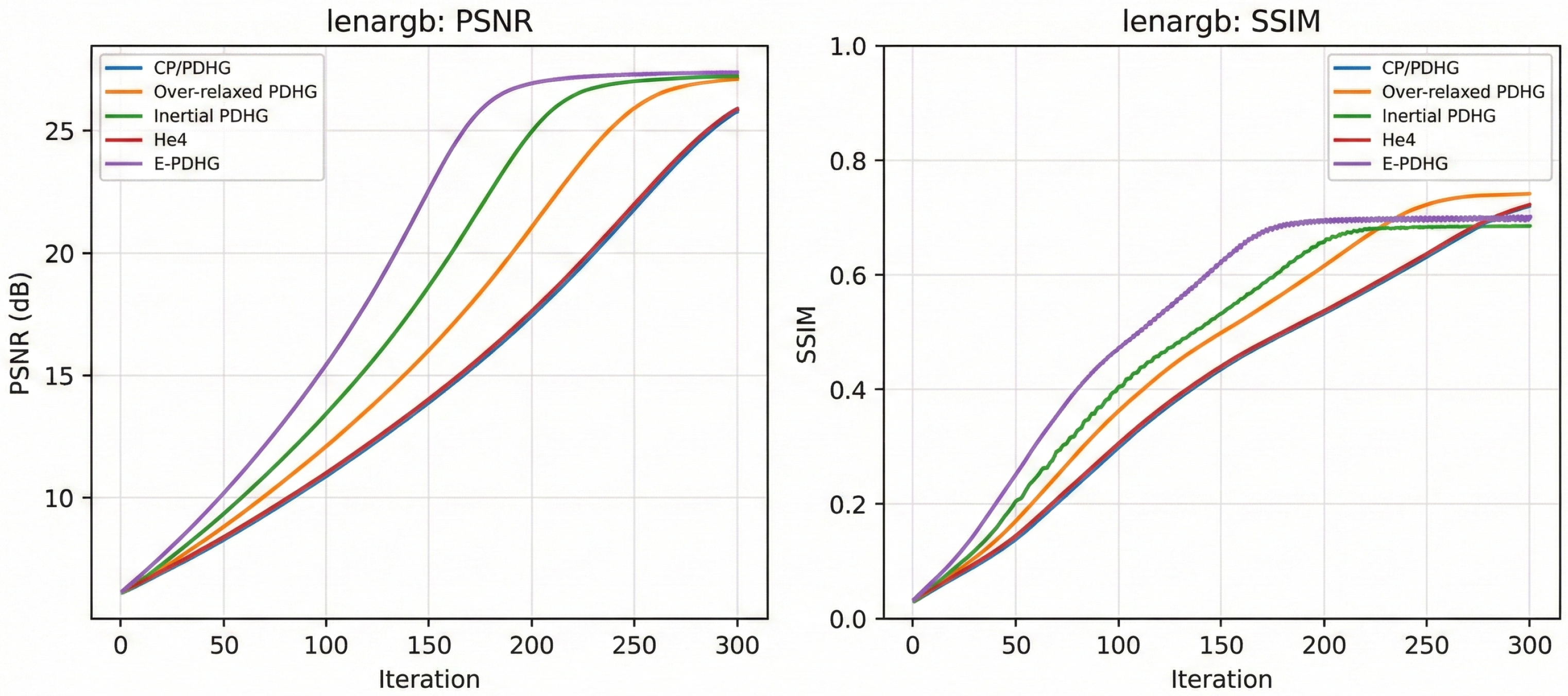
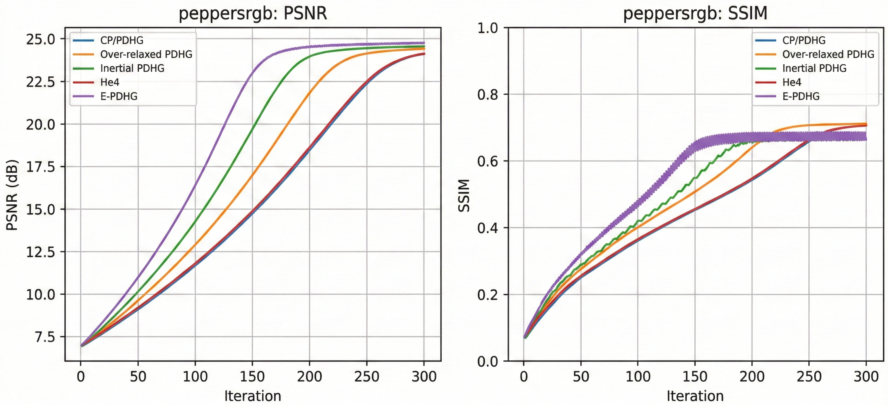
The results are reported in Figure 4 and Figure 5 with fixed 300 iterations.

Table 6. Inpainting results on lena.png ($512\times 512$).

Method	Final PSNR	Final SSIM	Runtime (s)	Iteration No.
E-PDHG	27.503	0.7124	60.19	181
Inertial PDHG	27.241	0.6855	96.79	302
Over-relaxed PDHG	27.125	0.7412	80.21	244
He4	25.901	0.7218	79.52	239
CP/PDHG	25.816	0.7202	113.71	341

and

Table 7. Inpainting results on peppers.png ($512\times 512$).

Method	Final PSNR	Final SSIM	Runtime (s)	Iteration No.
E-PDHG	24.829	0.6655	72.96	219
Inertial PDHG	24.567	0.6650	94.81	287
Over-relaxed PDHG	24.434	0.7109	79.81	233
He4	24.137	0.7059	86.56	252
CP/PDHG	24.126	0.7056	78.49	237

adopt terminating strategy whenever

$$max\left\{{\displaystyle \frac{\parallel x^{k+1}-x^k\parallel }{max\{1,\parallel x^k\parallel \}}},{\displaystyle \frac{\parallel y^{k+1}-y^k\parallel }{max\{1,\parallel y^k\parallel \}}}\right\}\le {10}^{-5},$$

or if the maximum number of iterations $K_{max}=2000$ is reached.

Overall, E-PDHG achieves the best PSNR on both inpainting tasks (Table 6 and Table 7) while also delivering the shortest runtime among the compared methods. Although over-relaxed PDHG attains the highest SSIM in both cases, its PSNR is lower and its runtime is longer. The curve comparisons in Figure 4 and Figure 5 further indicate faster and more stable convergence for E-PDHG, suggesting a favorable accuracy–efficiency trade-off for inpainting.

5.2. Machine Learning Models and Experimental Setup

To present the machine learning evidence in a unified optimization form, we use the composite model

$$\underset{u\in {\mathbb{R}}^n}{min}\lambda {\parallel u\parallel }_1+h\left(Du\right),$$

(48)

with the equivalent saddle formulation

$$\underset{u\in {\mathbb{R}}^n}{min}\underset{p\in {\mathbb{R}}^m}{max}\lambda {\parallel u\parallel }_1+\langle Du,p\rangle -h^{*}\left(p\right).$$

(49)

The two task instances are

$$\mathrm{Logistic}:D=\mathrm{Diag}\left(y\right)A,h\left(z\right)=C\sum _{i=1}^{m}log(1+exp(-z_i));$$

$$\mathrm{LASSO}:D=A,h\left(z\right)={\displaystyle \frac{1}{2}}{\parallel z-b\parallel }_2^2.$$

Under (49), the E-PDHG iteration reads

$$\begin{array}{cc}\hfill {\tilde{p}}^k& = {\mathrm{prox}}_{\sigma h^{*}}(p^k+\sigma D{u}^k),\hfill \end{array}$$

(50)

$$\begin{array}{cc}\hfill {\overline{p}}^k& = {\tilde{p}}^k+\eta ({\tilde{p}}^k-p^k),\hfill \end{array}$$

(51)

$$\begin{array}{cc}\hfill u^{k+1}& = {\mathrm{prox}}_{{\tau \lambda \parallel ·\parallel }_1}(u^k-\tau D^{\top }{\overline{p}}^k),\hfill \end{array}$$

(52)

$$\begin{array}{cc}\hfill p^{k+1}& = {\overline{p}}^k+\sigma D(u^{k+1}-u^k).\hfill \end{array}$$

(53)

The primal subproblem has the closed form

$${\mathrm{prox}}_{{\tau \lambda \parallel ·\parallel }_1}\left(v\right)=\mathrm{soft}(v,\tau \lambda )=\mathrm{sign}\left(v\right)\odot max\left(\right|v|-\tau \lambda ,0).$$

(54)

For the LASSO dual block $h\left(z\right)={\displaystyle \frac{1}{2}}{\parallel z-b\parallel }_2^2$, we use

$${\mathrm{prox}}_{\sigma h^{*}}\left(v\right)={\displaystyle \frac{v-\sigma b}{1+\sigma }}.$$

(55)

For the logistic dual block $h\left(z\right)=C{\sum }_{i}log(1+exp(-z_i))$, each coordinate solves

$$log{\displaystyle \frac{C+p_i}{-p_i}}+{\displaystyle \frac{p_i-v_i}{\sigma }}=0,p_i\in (-C,0),i=1,\dots ,m,$$

(56)

and we compute (56) by projected Newton iterations.

5.2.1. LASSO

For LASSO, we use the same model templates (48)–(50) with $D=A$ and $h\left(z\right)={\displaystyle \frac{1}{2}}{\parallel z-b\parallel }_2^2$, and apply the protocol in

Table 8. Machine learning protocol used in the logistic and LASSO benchmarks.

Item	Logistic Benchmark	LASSO Benchmark
Dataset	scikit-learn breast-cancer benchmark (binary, pos_label $=1$)	scikit-learn diabetes benchmark
Feature map	square expansion: $[A,A^{\odot 2}]$	original tabular features
Split and seed	train/test $=80/20$, seed $=42$ for main run	train/test $=80/20$, seed $=42$ for main run
Regularization	$\lambda =0.05{\lambda }_{max}$, $C=1$	$\lambda =0.05{\lambda }_{max}$
Step-size baseline	$1/{\parallel D\parallel }_2$ with $D=\mathrm{Diag}\left(y\right)A$	$1/{\parallel A\parallel }_2$
Main-run iterations	400 max iterations; unified stopping with min_iter $=200$, window $=20$, rel_tol $=8\times {10}^{-4}$	fixed 100 iterations
Sensitivity protocol	seeds $\{42,\dots ,46\}$, step_scale in $[0.05,0.95]$ with 37 points; strict profile: CP $\eta =1$, OR $\alpha =1.2$, Inertial $\beta =\gamma =0.3$, Accelerated $\mu ={\lambda }_{min}\left(A^{\top }A\right)$, He4 $\rho =2$, E-PDHG $\eta =0.98$	same seeds and step_scale grid; same strict profile; Inertial uses training/validation-only response clipping patch (1–99%)
Sensitivity metric	validation prediction error (robust ratio/std/robust span)	validation objective (robust ratio/std/robust span)

. The compared methods are CP/PDHG, over-relaxed PDHG, inertial PDHG, accelerated PDHG, He4, and E-PDHG ($\eta =1$). Inertial PDHG uses a training/validation-only response clipping patch (1–99%) to control oscillation; final reported metrics remain on the original data domain. The time-to-target threshold is

$$F_{\mathrm{target}}=1.01\times \underset{i}{min}{F}_i=613157.172788.$$

Table 9. LASSO diabetes benchmark final metrics (objective-oriented view; ↓ means lower is better).

Method	Final Objective ↓	Test MSE ↓	Time-to-Target (Iter) ↓	Status
CP/PDHG	629,291.338974	2608.346882	62	not_improved
Over-relaxed PDHG	623,993.167845	2559.255929	50	improved
Inertial PDHG	693,598.619300	3187.486363	62	not_improved
Accelerated PDHG	607,086.309691	2319.255504	52	improved
He4	636,992.882136	2678.867570	62	not_improved
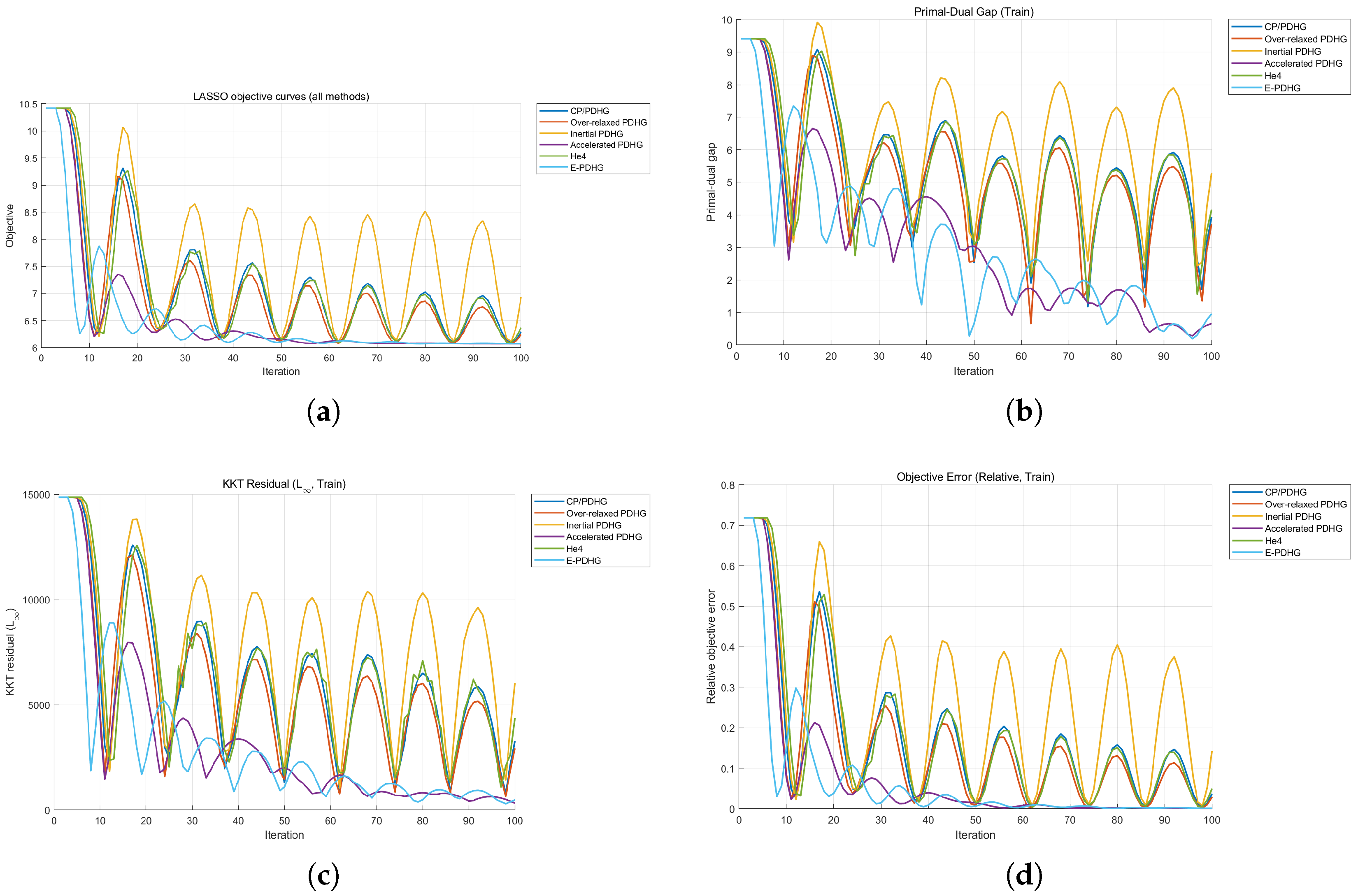
E-PDHG	607,281.120588	2364.870157	38	controlled

shows that E-PDHG reaches the target objective in the fewest iterations. Its final objective is close to the best value (accelerated PDHG), while test MSE remains comparable. This supports an objective- and time-to-target-oriented advantage in this sparse-regression setting. Figure 6 reports the full LASSO benchmark trajectories for the six compared methods.

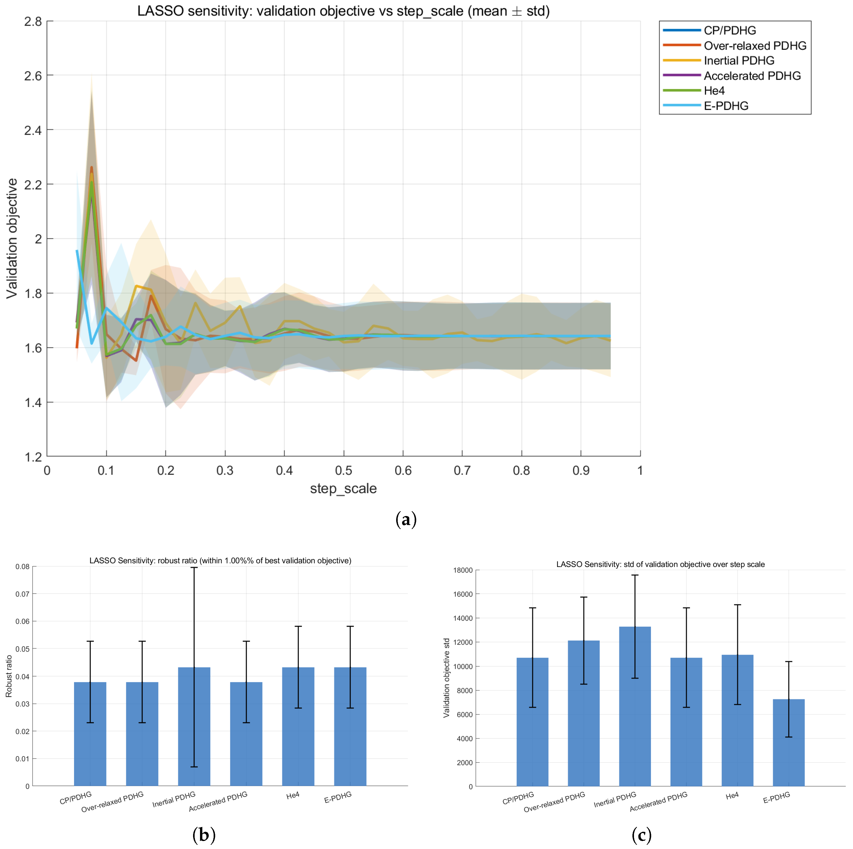
Under the same strict step_scale-only profile in Table 8, we further evaluate LASSO parameter robustness with the validation objective as the scoring quantity. The results indicate that E-PDHG keeps lower objective fluctuation while maintaining a competitive robust region. Figure 7 summarizes the corresponding LASSO sensitivity evidence across the scanned step-scale grid.

5.2.2. Logistic Classification

Using (48)–(50) and the protocol in Table 8, we compare CP/PDHG, over-relaxed PDHG, inertial PDHG, accelerated PDHG, He4, and E-PDHG ($\eta =1$) on the breast-cancer task. Notice that the problem is no longer strongly convex; hence, accelerated PDHG does not guarantee convergence. All methods stop at iteration 200 in this setting and attain the same predictive quality (test accuracy $=0.9737$, precision $=0.9740$, recall $=0.9868$, F1 $=0.9804$). Hence, the comparison is determined by optimization quality indicators under matched prediction metrics.

Table 10. Logistic benchmark final metrics (same prediction quality across methods; ↓ means lower is better).

Method	Test Objective ↓	PD Gap ↓	KKT∞ ↓	ObjErrrel ↓
CP/PDHG	84.2504	1.5976	0.6002	0.00354
Over-relaxed PDHG	84.3476	1.4448	0.6044	0.00445
Inertial PDHG	84.2558	1.6216	0.6125	0.00355
Accelerated PDHG	84.2503	1.5978	0.6003	0.00354
He4	84.2528	1.6023	0.6003	0.00357
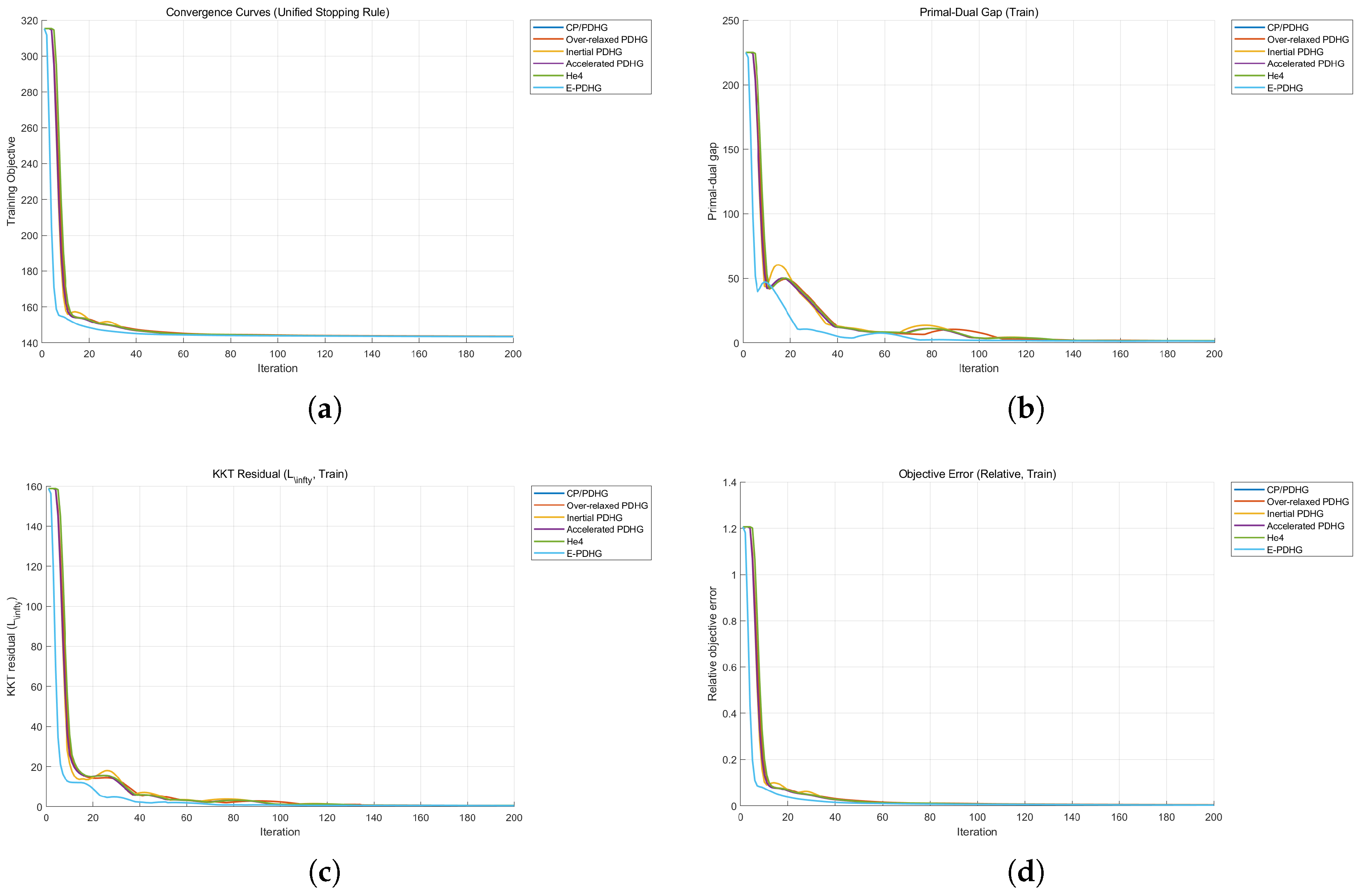
E-PDHG	84.2043	1.2759	0.4988	0.00325

shows that, at matched classification quality, E-PDHG attains the smallest objective value and the lowest residual-style indicators. This indicates better optimization accuracy for the same predictive operating point. Figure 8 shows the corresponding optimization trajectories for the logistic benchmark.

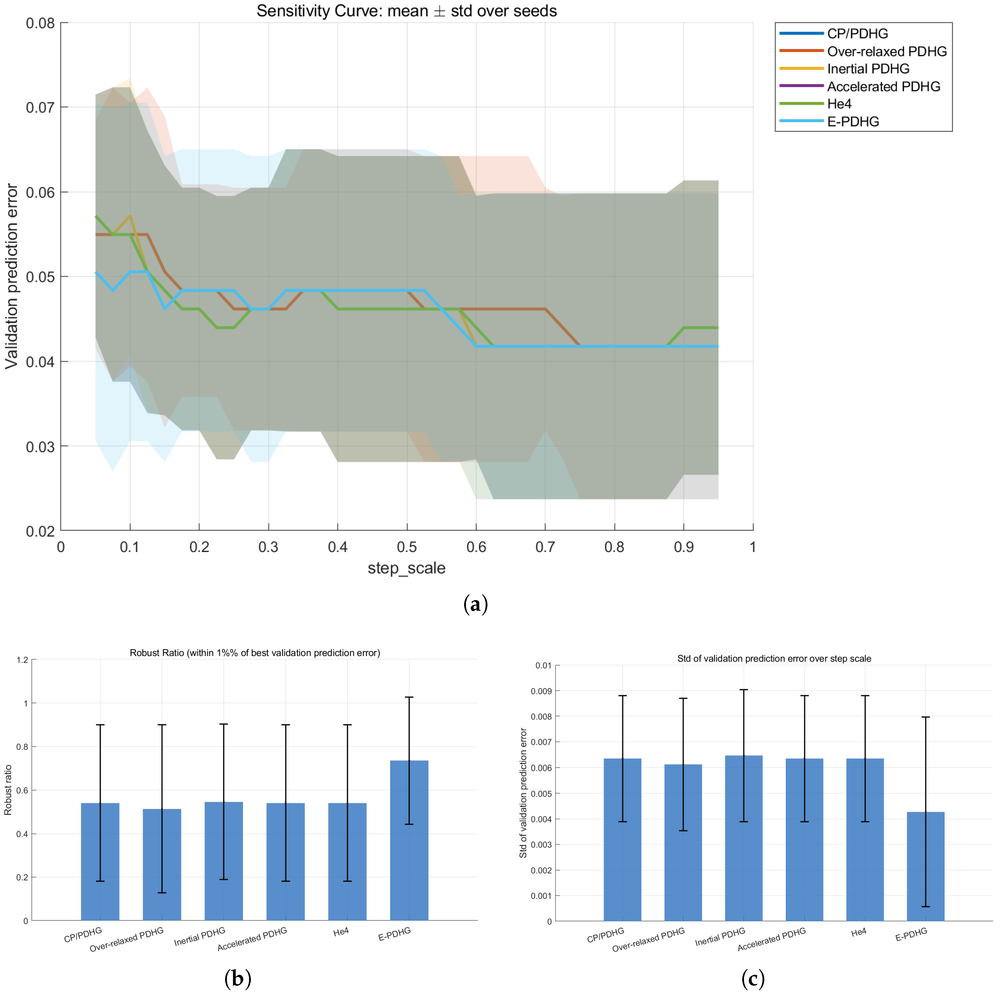
We next evaluate parameter robustness under the strict profile listed in Table 8. Let S be the scanned step_scale grid, $e\left(s\right)$ the validation prediction error at $s\in S$, and $e^{*}={min}_{s\in S}e\left(s\right)$. The reported indicators are

$$\mathrm{robust}\mathrm{ratio}={\displaystyle \frac{\left|\right\{s\in S:e\left(s\right)\le 1.01e^{*}\left\}\right|}{\left|S\right|}},\mathrm{pred}\text{-}\mathrm{err}\mathrm{std}=\mathrm{std}\{e\left(s\right):s\in S\},$$

and normalized robust span over the accepted set.

As summarized in

Table 11. Sensitivity summary (mean over five seeds; ↑ means higher is better and ↓ means lower is better).

Method	Robust Ratio ↑	PredErr Std ↓	Robust Span ↑
CP/PDHG	0.5405	0.0063	0.5889
Over-relaxed PDHG	0.5135	0.0061	0.5833
Inertial PDHG	0.5459	0.0065	0.5944
Accelerated PDHG	0.5405	0.0063	0.5889
He4	0.5405	0.0063	0.5889
E-PDHG	0.7351	0.0043	0.7389

, E-PDHG has the largest robust region and the smallest fluctuation over the scanned grid in this protocol. These statistics support a stronger parameter robustness trend for E-PDHG in this logistic task. Figure 9 displays the corresponding logistic sensitivity evidence over the scanned step-scale grid.

The machine learning results extend the empirical scope beyond imaging to classification and sparse regression, while keeping a single first-order primal-dual implementation framework. Across logistic and LASSO protocols, the comparisons are reported with both prediction-side and optimization-side indicators, enabling direct operational interpretation.

From a complexity perspective, these results are interpreted conservatively. We do not claim an improved asymptotic order over standard PDHG in the convex regime; the contribution is a symmetry-preserving correction mechanism that improves finite-iteration stability and objective-side quality under comparable predictive performance.

For reproducible use, the experiments provide a practical default: E-PDHG with fixed $\eta =0.98$ and moderate step scale is a stable baseline choice, and remains competitive without aggressive parameter search.

6. Conclusions

We presented E-PDHG, a symmetry-preserving refinement of PDHG that combines dual-side extrapolation with an explicit correction step. The method keeps the same low-cost proximal structure as standard PDHG while restoring primal-dual symmetry.

Theoretical analysis establishes global convergence for all $\eta \in (-1,1)$ under standard step-size conditions and provides a pointwise (non-ergodic) $O(1/\sqrt{t})$ rate for the last iterate. These results clarify the intermediate extrapolation regime without claiming any improvement in asymptotic complexity order.

Empirically, we expanded evaluation beyond imaging by adding logistic regression and LASSO benchmarks with unified protocols. Across deblurring, inpainting, and machine learning tasks, E-PDHG shows improved finite-iteration stability and competitive accuracy under comparable per-iteration cost. The sensitivity studies further support robust behavior near $\eta$ close to 1 within the admissible range.

Future work includes adaptive step-size strategies, extensions to strongly convex or nonconvex settings, and stochastic or large-scale variants.

References

1. Chambolle, A.; Pock, T. An introduction to continuous optimization for imaging. Acta Numer. 2016, 25, 161–319. [Google Scholar] [CrossRef] [Scilit]
2. Weiss, P.; Blanc-Feraud, L.; Aubert, G. Efficient schemes for total variation minimization under constraints in image processing. SIAM J. Sci. Comput. 2009, 31, 2047–2080. [Google Scholar] [CrossRef] [Scilit]
3. Zhu, M.; Chan, T.F. An Efficient Primal-Dual Hybrid Gradient Algorithm for Total Variation Image Restoration; CAM Report 08-34; UCLA: Los Angeles, CA, USA, 2008. [Google Scholar]
4. Chambolle, A.; Pock, T. A first-order primal-dual algorithms for convex problem with applications to imaging. J. Math. Imaging Vis. 2011, 40, 120–145. [Google Scholar]
5. Pock, T.; Chambolle, A. Diagonal preconditioning for first order primal-dual algorithms in convex optimization. In Proceedings of the IEEE International Conference on Computer Vision, Barcelona, Spain, 6–13 November 2011; pp. 1762–1769. [Google Scholar]
6. He, B.S.; Yuan, X.M. Convergence analysis of primal-dual algorithms for a saddle-point problem: From contraction perspective. SIAM J. Imaging Sci. 2012, 5, 119–149. [Google Scholar]
7. Goldstein, T.; Li, M.; Yuan, X.M.; Esser, E.; Baraniuk, R. Adaptive primal-dual hybrid gradient methods for saddle-point problems. arXiv 2013, arXiv:1305.0546. [Google Scholar]
8. O’Connor, D.; Vandenberghe, L. On the equivalence of the primal-dual hybrid gradient method and Douglas–Rachford splitting. Math. Prog. 2020, 179, 85–108. [Google Scholar]
9. Arrow, K.J.; Hurwicz, L.; Uzawa, H. Studies in Linear and Non-Linear Programming; With contributions by Chenery, H.B., Johnson, S.M., Karlin, S., Marschak, T. and Solow, R.M.; Stanford Mathematical Studies in the Social Science; Stanford University Press: Stanford, CA, USA, 1958; Volume II. [Google Scholar]
10. He, B.S.; You, Y.F.; Yuan, X.M. On the convergence of primal-dual hybrid gradient algorithm. SIAM J. Imaging Sci. 2014, 7, 2526–2537. [Google Scholar] [CrossRef] [Scilit]
11. He, B.S. PPA-like contraction methods for convex optimization: A framework using variational inequality approach. J. Oper. Res. Soc. China 2015, 3, 391–420. [Google Scholar] [CrossRef] [Scilit]
12. Condat, L. A primal-dual splitting method for convex optimization involving Lipschitzian, proximable and linear composite terms. J. Optim. Theory Appl. 2013, 158, 460–479. [Google Scholar] [CrossRef] [Scilit]
13. Cai, X.; Han, D.; Xu, L. An improved first-order primal-dual algorithm with a new correction step. J. Glob. Optim. 2013, 57, 1419–1428. [Google Scholar]
14. Lorenz, D.A.; Pock, T. An inertial forward-backward algorithm for monotone inclusions. J. Math. Imaging Vis. 2015, 51, 311–325. [Google Scholar] [CrossRef] [Scilit]
15. Boţ, R.I.; Csetnek, E.R. An inertial forward-backward-forward primal-dual splitting algorithm for solving monotone inclusion problems. Numer. Algorithms 2016, 71, 519–540. [Google Scholar]
16. Valkonen, T. Inertial, corrected, primal-dual proximal splitting. SIAM J. Optim. 2020, 30, 1391–1420. [Google Scholar] [CrossRef] [Scilit]
17. Chambolle, A.; Pock, T. On the ergodic convergence rates of a first-order primal-dual algorithm. Math. Prog. 2016, 159, 253–287. [Google Scholar]
18. Valkonen, T.; Pock, T. Acceleration of the PDHGM on partially strongly convex functions. J. Math. Imaging Vis. 2017, 59, 394–414. [Google Scholar] [CrossRef] [Scilit]
19. He, B.; Tao, M.; Yuan, X. Alternating direction method with Gaussian back substitution for separable convex programming. SIAM J. Optim. 2012, 22, 313–340. [Google Scholar] [CrossRef] [Scilit]
20. He, B.; Liu, H.; Wang, Z.; Yuan, X. A strictly contractive Peaceman–Rachford splitting method for convex programming. SIAM J. Optim. 2014, 24, 1011–1040. [Google Scholar]
21. He, B.S.; Ma, F.; Yuan, X.M. An algorithmic framework of generalized primal-dual hybrid gradient methods for saddle point problems. J. Math. Imaging Vis. 2017, 58, 279–293. [Google Scholar] [CrossRef] [Scilit]
22. Wu, J.; Ma, F. A primal-dual algorithm with coupled extrapolation: Bridging the Chambolle–Pock and Peaceman–Rachford methods. Numer. Algorithms 2025, 1–39. [Google Scholar] [CrossRef] [Scilit]
23. Ma, F.; Li, S.; Zhang, X. A symmetric version of the generalized Chambolle-Pock-He-Yuan method for saddle point problems. Comput. Optim. Appl. 2025, 1–26. [Google Scholar]
24. Ma, F. A revisit of Chen-Teboulle’s proximal-based decomposition method. arXiv 2020, arXiv:2006.11255. [Google Scholar] [CrossRef] [Scilit]
25. He, B.; Ma, F.; Xu, S.; Yuan, X. A rank-two relaxed parallel splitting version of the augmented Lagrangian method with step size in (0, 2) for separable convex programming. Math. Comput. 2023, 92, 1633–1663. [Google Scholar] [CrossRef] [Scilit]
26. Ma, S.; Li, S.; Ma, F. Preconditioned golden ratio primal-dual algorithm with linesearch. Numer. Algorithms 2025, 98, 1281–1311. [Google Scholar] [CrossRef] [Scilit]
27. Esser, E.; Zhang, X.; Chan, T.F. A general framework for a class of first order primal-dual algorithms for TV minimization. SIAM J. Imaging Sci. 2010, 3, 1015–1046. [Google Scholar] [CrossRef] [Scilit]
Figure 1. Left: original image; right: motion-blurred observation.
Axioms 15 00219 g001
Figure 2. Left: original image; right: Gaussian-blurred observation.
Axioms 15 00219 g002
Figure 3. From left to right: original lena.png ( 512 × 512 ), corrupted lena.png, original peppersrgb.png ( 512 × 512 ), and corrupted peppersrgb.png.
Axioms 15 00219 g003
Figure 4. Curve comparison (lenargb.png).
Axioms 15 00219 g004
Figure 5. Curve comparison (peppersrgb.png).
Axioms 15 00219 g005
Figure 6. Additional LASSO benchmark curves for the six methods (including He4): objective, primal-dual gap, KKT residual, and relative objective error. (a) Objective curve. (b) Primal-dual gap curve. (c) KKT residual curve. (d) Relative objective error curve.
Axioms 15 00219 g006
Figure 7. Additional LASSO sensitivity evidence over five seeds under strict step-scale-only profiles (including He4). (a) Validation objective vs. step_scale. (b) Robust ratio (higher is better). (c) Validation objective std (lower is better).
Axioms 15 00219 g007
Figure 8. Additional logistic benchmark curves for the six methods (including He4). (a) Training objective curve. (b) Primal-dual gap curve. (c) KKT residual curve. (d) Relative objective error curve.
Axioms 15 00219 g008
Figure 9. Additional logistic sensitivity evidence over five seeds (including He4). (a) Validation prediction error vs. step_scale. (b) Robust ratio (higher is better). (c) Prediction error std (lower is better).
Axioms 15 00219 g009