The Unit Arcsine–Exponential Distribution and Its Statistical Properties with Inference and Application to Reliability Data

Abstract

This paper presents a new continuous data model, the Unit Arcsine–Exponential distribution (UASED), a flexible data model on the unit interval. It is built up by an exponential-based arcsine-type transformation to allow it to represent a very wide range of shapes that can be used to model proportions and rates. A number of basic properties are obtained, such as closed-form formulas of the quantile function, moments, and entropy measures. Maximum likelihood and maximum product of spacings methods are developed to estimate parameters, and their performance is determined by Monte Carlo simulation, which shows that these methods can reasonably estimate the parameters and be stable over a variety of different parameter settings. To demonstrate that a model is practically useful, an application to real-world data on the reliability of devices in terms of failure time is discussed. The findings indicate that the UASED is a good fit to the data, in the sense that it is effective in terms of skewness and tail behavior and compares well or competes favorably with current unit distributions. All in all, the suggested model is a sparse alternative to model bounded data with sound inferential characteristics and high practical utility.

1. Motivation and Introduction

Statistical analysis on data restricted to the unit interval $(0,1)$ is a key aspect of most scientific fields, such as reliability engineering, economics, environmental science, medicine, and social sciences. This type of data is usually in the form of proportions, rates, indexes, probabilities, and normalized measurements. In this case, classical unbounded distributions cannot be used, but they do not allow for the natural limits of the data to be taken into account, which is why flexible unit-interval distributions are developed.

The beta distribution, which was first introduced in [1], has long been a paradigm of bounded data due to the remarkable ability of the distribution to capture a wide variety of distributional forms. Its reliance on special functions can, however, carry considerable computation challenges, particularly in estimating parameters, as well as in the analysis of quantiles. These limitations have led to the design of other unit-interval distributions that are analytically more tractable. Some of them include the Kumaraswamy distribution, in which the analysis was carried out in [2]; the Topp–Leone distribution, which was introduced in [3]; and the power distributions proposed in [4], which have numerous generalizations. In the recent past, it has moved toward building unit distributions based on transformation. These methods take exponential, reciprocal, logit, and other functional forms and projections of known lifetime distributions to model flexible and analytically computable models.

The most successful of these methods is the exponential transformation $Y=e^{-X}$, with X a non-negative continuous random variable, used to build the models that are bounded. This approach retains the tractability in the analysis, but it imposes rich distributional forms on the unit interval. It has given rise to a number of successful unit distributions, such as the unit inverse Gaussian in [5], the unit Lindley in [6], the unit Weibull in [7], the unit Gompertz in [8], the unit gamma intensively discussed in [9], and other unit models. These distributions have proven to be quite effective in the modeling of skewed unit data, as well as in the modeling of the various behaviors of hazard rates.

Lifetime distributions play a fundamental role in reliability theory and survival analysis, where the ability to model diverse hazard-rate behaviors is crucial. In this context, the Arcsine–Exponential distribution (ASED) with one parameter $\lambda$, denoted by $\mathrm{ASED}\left(\lambda \right)$, which was first introduced in [10], has recently gained widespread popularity due to its manipulatory form and distinctive probabilistic properties. Despite its high effectiveness with non-negative data, its unlimited range restricts its direct application to proportion-type datasets, thereby motivating the development of a unit-interval equivalent. For any continuous random variable $X\sim \mathrm{ASED}\left(\lambda \right)$, the cumulative distribution function (CDF) and probability density function (PDF) are expressed as

$$F_X(x;\lambda )={\displaystyle \frac{2}{\pi }}arcsin\left(\sqrt{1-e^{-\lambda x}}\right),x>0,\lambda >0,$$

(1)

and

$$f_X(x;\lambda )={\displaystyle \frac{\lambda \sqrt{e^{-\lambda x}}}{\pi \sqrt{1-e^{-\lambda x}}}},x>0,\lambda >0.$$

(2)

This study proposes a novel bounded probability distribution, named as the Unit Arcsine–Exponential distribution (UASED), obtained by applying the exponential transformation $Y=e^{-X}$ to a continuous random variable X following the ASED. The resulting distribution is supported on $(0,1)$ and retains the analytical tractability of the parent distribution and has better flexibility in the modeling of unit-interval data. The UASED can be defined with a single parameter, namely $\lambda$, but with a variety of density and hazard rate shapes, which makes it especially useful in the use of skewed proportions and phenomena related to reliability. The key contributions of the paper are the following:

(i)

To introduce a novel one-parameter unit distribution derived from the ASED;

(ii)

To obtain and analyze its basic statistical characteristics, such as the probability density function, distributional shapes, quantile function, moments, and entropy measures;

(iii)

To develop classical and Bayesian inference procedures for parameter estimation and assess their performance via simulation studies;

(iv)

To illustrate the practical utility of the proposed model through applications to real lifetime and proportion-type datasets.

The rest of this paper will be structured in the following way. Section 2 defines the UASED and its distributional forms. The statistical properties and the entropy measures of it are analyzed in Section 3. Section 4 is about non-Bayesian inference and gives likelihood-based and spacing-based methods of estimation and the associated asymptotic confidence interval. Section 5 lays the foundation of the Bayesian inference model, where both informative and non-informative priors are taken and estimation is performed using the Metropolis–Hastings algorithm. The effectiveness of the proposed methods is evaluated by a Monte Carlo simulation study in Section 6 of this paper. The specific application to real-world data in the section is contained in Section 7 of the paper to demonstrate the flexibility and usefulness of the model. Lastly, there is a conclusion to the paper in Section 8.

2. Unit Arcsine–Exponential Distribution

Let $X\sim \mathrm{ASED}\left(\lambda \right)$ with CDF as in Equation (1). To construct a unit-bounded distribution from the ASED, we apply the monotone decreasing transformation $Y=e^{-X}$. Since $X\in (0,\infty )$, it follows that $Y\in (0,1)$, and the inverse transformation is given by $X=-logY$. Then the CDF of Y can be derived as

$$\begin{array}{cc}\hfill F_Y(y;\lambda )& =\mathbb{P}(Y\le y)=\mathbb{P}(e^{-X}\le y)=\mathbb{P}(X\ge -logy)=1-F_X(-logy;\lambda )\hfill \\ \hfill & =1-{\displaystyle \frac{2}{\pi }}arcsin\left(\sqrt{1-e^{-\lambda (-logy)}}\right)\hfill \\ \hfill & =1-{\displaystyle \frac{2}{\pi }}arcsin\left(\sqrt{1-y^{\lambda }}\right),0<y<1,\lambda >0.\hfill \end{array}$$

(3)

Consequently, the transformed random variable Y is said to follow a UASED, denoted by $Y\sim \mathrm{UASED}\left(\lambda \right)$, with CDF given in Equation (3). The corresponding PDF is given by

$$f_Y(y;\lambda )={\displaystyle \frac{\lambda y^{\lambda -1}}{\pi \sqrt{y^{\lambda }\left(1-y^{\lambda }\right)}}},0<y<1,\lambda >0.$$

(4)

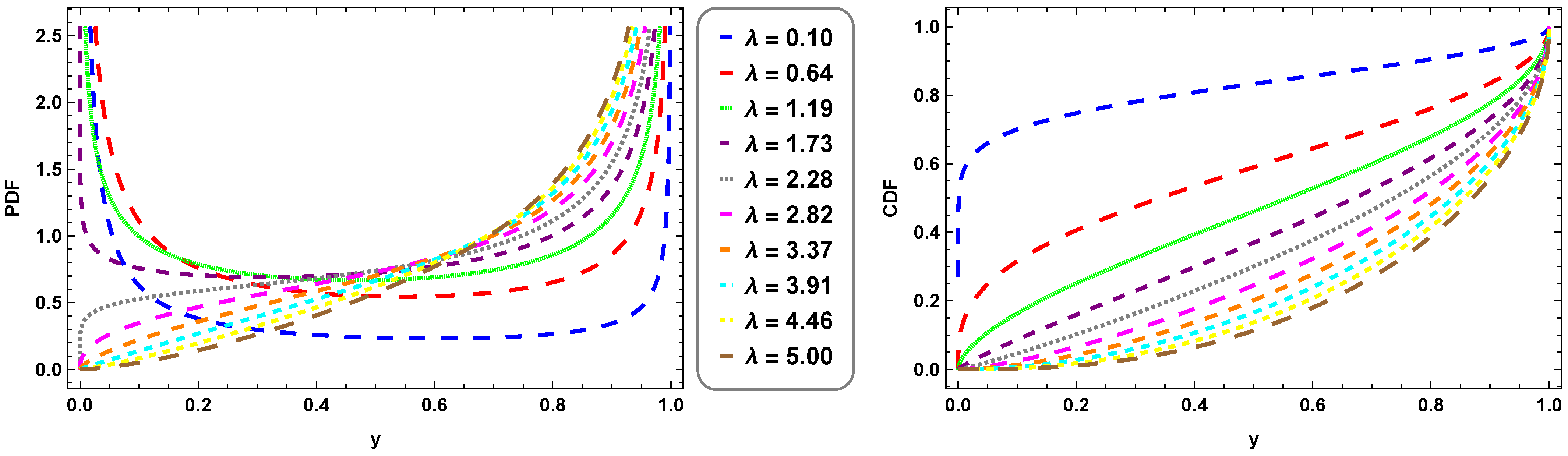
The PDF in Equation (4) is obtained by direct differentiation of the CDF in Equation (3) with respect to y, confirming that the UASED admits a closed-form density. Figure 1 shows the representative PDF and CDF curves of the various values of $\lambda$ that represent the flexibility of the proposed model on the unit interval. There is a change from a U-shaped distribution in small values to the J-shaped or left-skewed distribution in large values as $\lambda$ changes.

The reliability function (RF) of the random variable Y and associated hazard function (HF) are, respectively, as follows:

$$R_Y(y;\lambda )=1-F_Y(y;\lambda )={\displaystyle \frac{2}{\pi }}arcsin\left(\sqrt{1-y^{\lambda }}\right),0<y<1,$$

(5)

and

$$h_Y(y;\lambda )={\displaystyle \frac{f_Y(y;\lambda )}{R_Y(y;\lambda )}}={\displaystyle \frac{\lambda y^{\lambda -1}}{2\sqrt{y^{\lambda }(1-y^{\lambda })}arcsin\left(\sqrt{1-y^{\lambda }}\right)}},0<y<1.$$

(6)

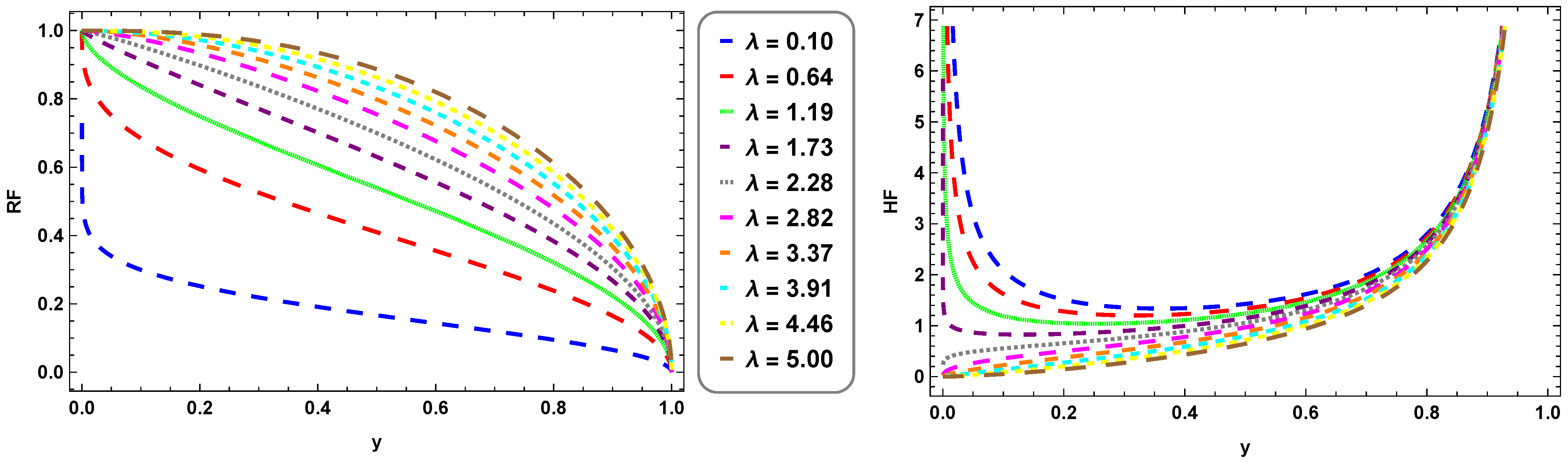
The UASED has some representative shapes of the RF and HF, as shown in Figure 2. The plot illustrates that the trend of the HF as a variable of the plot is generally increasing with the increase in the variable of the plot, which is y. Specifically, at smaller values of the parameter $\lambda$, the curves have the relatively flat or bathtub-shaped profiles, and at greater values of the parameter, the HF grows more rapidly, coming close to the exponential-like growth closer to the upper edge of the unit interval. This behavior highlights the flexibility of the UASED in modeling diverse reliability and lifetime patterns on the unit interval.

Remark 1. 

Let $Y\sim \mathrm{UASED}\left(\lambda \right)$ with PDF as in Equation (4). Then, by setting $\lambda =1$, the PDF reduces to that of the standard arcsine distribution (ASD) on $(0,1)$, i.e., $Y\sim \mathrm{Beta}\left(a,b\right)$ with $a=b={\displaystyle \frac{1}{2}}$.

3. Statistical Properties of the UASED

This section focuses on the derivation of important mathematical properties of the proposed UASED.

3.1. Identifiability Property and Mode

This subsection focuses on the identifiability property and the mode of the UASED. The shape parameter $\lambda$ is considered identifiable if equality of the CDFs necessarily implies equality of the corresponding parameters. The mode, representing the value at which the PDF attains its maximum, characterizes the boundary behavior of the distribution and depends solely on $\lambda$.

Theorem 1 (Identifiability of the UASED Parameter).

Let $Y\sim \mathrm{UASED}\left(\lambda \right)$ with CDF given in Equation (3). Then the parameter λ is identifiable, that is, $F_Y(y;{\lambda }_1)=F_Y(y;{\lambda }_2)$ for all $y\in (0,1)$ implies that ${\lambda }_1={\lambda }_2.$

Proof. 

Suppose that two parameters ${\lambda }_1$ and ${\lambda }_2$ produce the same CDF:   

$$\begin{array}{cc}\hfill F_Y(y;{\lambda }_1)& =F_Y(y;{\lambda }_2),\hfill \\ \hfill 1-{\displaystyle \frac{2}{\pi }}arcsin\left(\sqrt{1-y^{{\lambda }_1}}\right)& =1-{\displaystyle \frac{2}{\pi }}arcsin\left(\sqrt{1-y^{{\lambda }_2}}\right),\hfill \\ \hfill arcsin\left(\sqrt{1-y^{{\lambda }_1}}\right)& =arcsin\left(\sqrt{1-y^{{\lambda }_2}}\right),\hfill \\ \hfill \sqrt{1-y^{{\lambda }_1}}& =\sqrt{1-y^{{\lambda }_2}},\hfill \\ \hfill 1-y^{{\lambda }_1}& =1-y^{{\lambda }_2},\hfill \\ \hfill y^{{\lambda }_1}& =y^{{\lambda }_2},0<y<1.\hfill \end{array}$$

Since this equality holds for all $y\in (0,1)$, it follows immediately that ${\lambda }_1={\lambda }_2$. Thus, the UASED is identifiable with respect to the parameter $\lambda$.    □

Theorem 2 (Mode of the UASED).

Let $Y\sim \mathrm{UASED}\left(\lambda \right)$ with PDF given in Equation (4). The mode of Y is determined as follows:

1. 

For $0<\lambda <2$, the PDF is U-shaped and bimodal, with modes occurring at the boundaries $y\to 0^{+}$ and $y\to 1^{-}$. In this case, there exists an anti-mode (local minimum) at $y^{*}={\left(1-{\displaystyle \frac{\lambda }{2}}\right)}^{\frac{1}{\lambda }}$.

2. 

For $\lambda \ge 2$, the PDF is strictly increasing on $(0,1)$, so the unique mode is located at the right boundary $y\to 1^{-}$.

Proof. 

To find the critical points, differentiate the PDF $f_Y(y;\lambda )$ in Equation (4) with respect to y and set $f_Y^{\prime }(y;\lambda )=0$. This yields $(\lambda -2)(1-y^{\lambda })+\lambda y^{\lambda }=0,$ which gives the interior critical point $y^{*}={\left(1-{\displaystyle \frac{\lambda }{2}}\right)}^{\frac{1}{\lambda }}.$ Analyzing this point based on $\lambda$:

• For $0<\lambda <2$, we have $y^{*}\in (0,1)$. Examining $f_Y^{\prime }(y;\lambda )$ shows $f_Y^{\prime }(y;\lambda )<0$ for $y<y^{*}$ and $f_Y^{\prime }(y;\lambda )>0$ for $y>y^{*}$, indicating that $y^{*}$ is a local minimum (anti-mode). Since $f_Y(y;\lambda )\to \infty$ as $y\to 0^{+}$ and $y\to 1^{-}$, the PDF is U-shaped with modes at the boundaries.
• For $\lambda \ge 2$, no solution exists in $(0,1)$ because $1-{\displaystyle \frac{\lambda }{2}}\le 0$. Here, $f_Y^{\prime }(y;\lambda )>0$ for all $y\in (0,1)$, implying that the PDF is strictly increasing. Thus, the mode occurs at the right boundary: $y_{\mathrm{mode}}=1$.

   □

3.2. Quantile Function and Random Sample Generation

This subsection focuses on deriving the quantile function and using it to simulate random samples from the proposed UASED.

Theorem 3 (Quantile Function of the UASED).

Let $Y\sim \mathrm{UASED}\left(\lambda \right)$ with CDF given in Equation (3). The quantile function (QF) of Y, denoted by $Q_Y(q;\lambda )$ for $0<q<1$, is obtained as the inverse of the CDF:

$$Q_Y(q;\lambda )={\left[sin\left({\displaystyle \frac{\pi }{2}}q\right)\right]}^{{\displaystyle \frac{2}{\lambda }}}.$$

(7)

Proof. 

By definition, the QF is the inverse of the CDF:

$$Q_Y(q;\lambda )=F_Y^{-1}(q;\lambda ),0<q<1.$$

From Equation (3), by setting the CDF $F_Y(y;\lambda )=q$ and solving for y, we obtain

$$q=1-{\displaystyle \frac{2}{\pi }}arcsin\left(\sqrt{1-y^{\lambda }}\right),\mathrm{so}\mathrm{that}arcsin\left(\sqrt{1-y^{\lambda }}\right)={\displaystyle \frac{\pi }{2}}(1-q)={\displaystyle \frac{\pi }{2}}-{\displaystyle \frac{\pi }{2}}q.$$

Applying the sine function to both sides yields

$$\sqrt{1-y^{\lambda }}=cos\left({\displaystyle \frac{\pi }{2}}q\right),\mathrm{so}\mathrm{that}{y}^{\lambda }=1-{cos}^2\left({\displaystyle \frac{\pi }{2}}q\right)={sin}^2\left({\displaystyle \frac{\pi }{2}}q\right),\mathrm{and}\mathrm{thus},$$

$$Q_Y(q;\lambda )=y={\left[sin\left({\displaystyle \frac{\pi }{2}}q\right)\right]}^{{\displaystyle \frac{2}{\lambda }}},$$

which completes the proof.    □

Remark 2 (Quartiles and Median of the UASED).

For the UASED, the first quartile ($Q_1$), median ($Q_2$), and third quartile ($Q_3$) correspond to the 25th, 50th, and 75th percentiles of the distribution, respectively. These can be obtained directly from the quantile function by setting $q=0.25$, $0.50$, and $0.75$:

$$Q_1=Q_Y\left(0.25\right),Q_2=Q_Y\left(0.50\right),Q_3=Q_Y\left(0.75\right).$$

Remark 3 (Random Sample Generation via Inverse Transform).

A uniform random variable $u\sim \mathrm{U}[0,1]$ can be transformed into a UASED random variable using the inverse transform method:

$$Y={\left[sin\left({\displaystyle \frac{\pi }{2}}u\right)\right]}^{{\displaystyle \frac{2}{\lambda }}}.$$

(8)

The random samples of Y can be generated efficiently to conduct a simulation study, Monte Carlo experiment, or statistical estimation through generating independent values of u and using Equation (8) to generate random samples of $Y\sim \mathrm{UASED}\left(\lambda \right)$.

3.3. Moments and Related Statistical Quantities

This subsection focuses on obtaining the moments, central moments, moment generating function, characteristic function, cumulant generating function, and incomplete moments for the proposed UASED, as well as the computation and discussion of key associated measures: mean, variance, skewness, kurtosis, and coefficient of variation.

Theorem 4 (Moments of the UASED).

Let $Y\sim \mathrm{UASED}\left(\lambda \right)$ with PDF given in Equation (4). Then the $r^{th}$ non-central moment of Y exists and is given by

$${\mu }_r^{\prime }=\mathbb{E}\left[Y^r\right]={\displaystyle \frac{1}{\sqrt{\pi }}}{\displaystyle \frac{\mathsf{\Gamma }\left(\frac{r}{\lambda }+\frac{1}{2}\right)}{\mathsf{\Gamma }\left(\frac{r}{\lambda }+1\right)}},r>-{\displaystyle \frac{\lambda }{2}}.$$

(9)

Proof. 

By definition, the $r^{th}$ non-central moment of Y is

$${\mu }_r^{\prime }=\mathbb{E}\left[Y^r\right]={\int }_0^1{y}^r{f}_Y(y;\lambda )dy={\displaystyle \frac{\lambda }{\pi }}{\int }_0^1{\displaystyle \frac{y^{r+\lambda -1}}{\sqrt{y^{\lambda }(1-y^{\lambda })}}}dy={\displaystyle \frac{\lambda }{\pi }}{\int }_0^1{y}^{r+\lambda /2-1}{(1-y^{\lambda })}^{-1/2}dy.$$

Using the transformation $t=y^{\lambda }$, $dy={\displaystyle \frac{1}{\lambda }}{t}^{\frac{1}{\lambda }-1}dt$, the integral becomes

$${\mu }_r^{\prime }={\displaystyle \frac{1}{\pi }}{\int }_0^1{t}^{\frac{r}{\lambda }-\frac{1}{2}}{(1-t)}^{-1/2}dt.$$

Recognizing this integral as the Beta function $B(a,b)={\int }_0^1{t}^{a-1}{(1-t)}^{b-1}dt$, we obtain

$${\mu }_r^{\prime }={\displaystyle \frac{1}{\pi }}B\left({\displaystyle \frac{r}{\lambda }}+{\displaystyle \frac{1}{2}},{\displaystyle \frac{1}{2}}\right),r>-{\displaystyle \frac{\lambda }{2}}.$$

Finally, using $B(a,b)={\displaystyle \frac{\mathsf{\Gamma }\left(a\right)\mathsf{\Gamma }\left(b\right)}{\mathsf{\Gamma }(a+b)}}$ and $\mathsf{\Gamma }(1/2)=\sqrt{\pi }$, we arrive at

$${\mu }_r^{\prime }={\displaystyle \frac{1}{\sqrt{\pi }}}{\displaystyle \frac{\mathsf{\Gamma }\left(\frac{r}{\lambda }+\frac{1}{2}\right)}{\mathsf{\Gamma }\left(\frac{r}{\lambda }+1\right)}},r>-{\displaystyle \frac{\lambda }{2}},$$

which completes the proof.    □

Theorem 5 (Central Moments of the UASED).

Let $Y\sim \mathrm{UASED}\left(\lambda \right)$ with PDF given in Equation (4), and let $\mu =\mathbb{E}\left[Y\right]$ be its mean. Then the $r^{th}$ central moment of Y is

$${\mu }_r=\mathbb{E}\left[{(Y-\mu )}^r\right]={\displaystyle \frac{1}{\sqrt{\pi }}}\sum _{k=0}^r\left({\displaystyle \genfrac{}{}{0pt}{}{r}{k}}\right){(-1)}^{r-k}{\mu }^{r-k}{\displaystyle \frac{\mathsf{\Gamma }\left(\frac{k}{\lambda }+\frac{1}{2}\right)}{\mathsf{\Gamma }\left(\frac{k}{\lambda }+1\right)}},r\ge 1.$$

(10)

Proof. 

By definition, the $r^{th}$ central moment of Y is

$${\mu }_r=\mathbb{E}\left[{(Y-\mu )}^r\right]={\int }_0^1{(y-\mu )}^r{f}_Y(y;\lambda )dy.$$

Expanding ${(y-\mu )}^r$ using the binomial theorem gives

$${(y-\mu )}^r=\sum _{k=0}^r\left({\displaystyle \genfrac{}{}{0pt}{}{r}{k}}\right){(-1)}^{r-k}{\mu }^{r-k}{y}^k.$$

Substituting this expansion into the integral yields

$$\begin{array}{cc}\hfill {\mu }_r={\int }_0^1\sum _{k=0}^r\left({\displaystyle \genfrac{}{}{0pt}{}{r}{k}}\right){(-1)}^{r-k}{\mu }^{r-k}{y}^k{f}_Y(y;\lambda )dy& =\sum _{k=0}^r\left({\displaystyle \genfrac{}{}{0pt}{}{r}{k}}\right){(-1)}^{r-k}{\mu }^{r-k}{\int }_0^1{y}^k{f}_Y(y;\lambda )dy\hfill \\ & =\sum _{k=0}^r\left({\displaystyle \genfrac{}{}{0pt}{}{r}{k}}\right){(-1)}^{r-k}{\mu }^{r-k}{\mu }_k^{\prime }.\hfill \end{array}$$

Substituting the expression for the $k^{th}$ non-central moment from Equation (9), we obtain

$${\mu }_r={\displaystyle \frac{1}{\sqrt{\pi }}}\sum _{k=0}^r\left({\displaystyle \genfrac{}{}{0pt}{}{r}{k}}\right){(-1)}^{r-k}{\mu }^{r-k}{\displaystyle \frac{\mathsf{\Gamma }\left(\frac{k}{\lambda }+\frac{1}{2}\right)}{\mathsf{\Gamma }\left(\frac{k}{\lambda }+1\right)}},$$

which completes the proof.    □

Remark 4 (Descriptive Measures of the UASED).

The mean, variance, skewness, kurtosis, coefficient of variation, and coefficient of dispersion summarize the central tendency, variability, asymmetry, and tail behavior of the UASED. For $Y\sim \mathrm{UASED}\left(\lambda \right)$, the principal descriptive measures are given by:

• Mean:

  $$\mu ={\mu }_1^{\prime }=\mathbb{E}\left[Y\right]={\displaystyle \frac{1}{\sqrt{\pi }}}{\displaystyle \frac{\mathsf{\Gamma }\left(\frac{1}{\lambda }+\frac{1}{2}\right)}{\mathsf{\Gamma }\left(\frac{1}{\lambda }+1\right)}}.$$
• Variance:

  $${\sigma }^2={\mu }_2={\mu }_2^{\prime }-{\mu }^2={\displaystyle \frac{1}{\sqrt{\pi }}}{\displaystyle \frac{\mathsf{\Gamma }\left(\frac{2}{\lambda }+\frac{1}{2}\right)}{\mathsf{\Gamma }\left(\frac{2}{\lambda }+1\right)}}-{\displaystyle \frac{1}{\pi }}{\displaystyle \frac{\mathsf{\Gamma }{\left(\frac{1}{\lambda }+\frac{1}{2}\right)}^2}{\mathsf{\Gamma }{\left(\frac{1}{\lambda }+1\right)}^2}}.$$
• Skewness:

  $$\begin{array}{cc}\hfill {\gamma }_1={\displaystyle \frac{{\mu }_3}{{\mu }_2^{3/2}}}& ={\displaystyle \frac{{\mu }_3^{\prime }-3{\mu }_1^{\prime }{\mu }_2^{\prime }+2{\left({\mu }_1^{\prime }\right)}^3}{{({\mu }_2^{\prime }-{\mu }^2)}^{3/2}}}=\left[2{\displaystyle \frac{\mathsf{\Gamma }{\left(\frac{1}{\lambda }+\frac{1}{2}\right)}^3}{\mathsf{\Gamma }{\left(\frac{1}{\lambda }+1\right)}^3}}-3\pi 4^{-\frac{1}{\lambda }}{\displaystyle \frac{\mathsf{\Gamma }\left(\frac{2}{\lambda }+\frac{1}{2}\right)}{\mathsf{\Gamma }{\left(\frac{1}{\lambda }+1\right)}^2}}\right.\hfill \\ & \left.+\pi {\displaystyle \frac{\mathsf{\Gamma }\left(\frac{3}{\lambda }+\frac{1}{2}\right)}{\mathsf{\Gamma }\left(\frac{3}{\lambda }+1\right)}}\right]\times {\left[\sqrt{\pi }{\displaystyle \frac{\mathsf{\Gamma }\left(\frac{2}{\lambda }+\frac{1}{2}\right)}{\mathsf{\Gamma }\left(\frac{2}{\lambda }+1\right)}}-{\displaystyle \frac{\mathsf{\Gamma }{\left(\frac{1}{\lambda }+\frac{1}{2}\right)}^2}{\mathsf{\Gamma }{\left(\frac{1}{\lambda }+1\right)}^2}}\right]}^{-\frac{3}{2}}.\hfill \end{array}$$
• Kurtosis:

  $$\begin{array}{cc}\hfill {\gamma }_2={\displaystyle \frac{{\mu }_4}{{\mu }_2^2}}-3& ={\displaystyle \frac{{\mu }_4^{\prime }-4\mu {\mu }_3^{\prime }+6{\mu }^2{\mu }_2^{\prime }-3{\mu }^4}{{({\mu }_2^{\prime }-{\mu }^2)}^2}}-3={\displaystyle \frac{\lambda }{\pi }}\left[-{\displaystyle \frac{3{\lambda }^3}{\pi }}{\displaystyle \frac{\mathsf{\Gamma }{\left(\frac{1}{\lambda }+\frac{1}{2}\right)}^4}{\mathsf{\Gamma }{\left(\frac{1}{\lambda }\right)}^4}}\right.\hfill \\ & +{\displaystyle \frac{2}{3}}\left(94^{-\frac{1}{\lambda }}{\displaystyle \frac{\mathsf{\Gamma }\left(\frac{2}{\lambda }+\frac{1}{2}\right)}{\mathsf{\Gamma }\left(\frac{1}{\lambda }\right)}}-2{\displaystyle \frac{\mathsf{\Gamma }\left(\frac{1}{\lambda }+1\right)\mathsf{\Gamma }\left(\frac{3}{\lambda }+\frac{1}{2}\right)}{\mathsf{\Gamma }\left(\frac{3}{\lambda }\right)}}\right){\displaystyle \frac{\mathsf{\Gamma }\left(\frac{1}{\lambda }+\frac{1}{2}\right)}{\mathsf{\Gamma }{\left(\frac{1}{\lambda }+1\right)}^2}}\hfill \\ & \left.+{\displaystyle \frac{\sqrt{\pi }}{4}}{\displaystyle \frac{\mathsf{\Gamma }\left(\frac{4}{\lambda }+\frac{1}{2}\right)}{\mathsf{\Gamma }\left(\frac{4}{\lambda }\right)}}\right]\times {\left[{\displaystyle \frac{1}{\pi }}{\displaystyle \frac{\mathsf{\Gamma }{\left(\frac{1}{\lambda }+\frac{1}{2}\right)}^2}{\mathsf{\Gamma }{\left(\frac{1}{\lambda }+1\right)}^2}}-{\displaystyle \frac{1}{\sqrt{\pi }}}{\displaystyle \frac{\mathsf{\Gamma }\left(\frac{2}{\lambda }+\frac{1}{2}\right)}{\mathsf{\Gamma }\left(\frac{2}{\lambda }+1\right)}}\right]}^{-2}-3.\hfill \end{array}$$
• Coefficient of Variation:

  $$\mathcal{CV}={\displaystyle \frac{\sigma }{\mu }}={\displaystyle \frac{\mathsf{\Gamma }\left(\frac{1}{\lambda }+1\right)}{\mathsf{\Gamma }\left(\frac{1}{\lambda }+\frac{1}{2}\right)}}\sqrt{\sqrt{\pi }{\displaystyle \frac{\mathsf{\Gamma }\left(\frac{2}{\lambda }+\frac{1}{2}\right)}{\mathsf{\Gamma }\left(\frac{2}{\lambda }+1\right)}}-{\displaystyle \frac{\mathsf{\Gamma }{\left(\frac{1}{\lambda }+\frac{1}{2}\right)}^2}{\mathsf{\Gamma }{\left(\frac{1}{\lambda }+1\right)}^2}}}.$$
• Coefficient of Dispersion:

  $$\mathcal{CD}={\displaystyle \frac{{\sigma }^2}{\mu }}={\displaystyle \frac{1}{\sqrt{\pi }\mathsf{\Gamma }{\left(\frac{1}{\lambda }+\frac{1}{2}\right)}^2}}\left[\pi 4^{-\frac{1}{\lambda }}\mathsf{\Gamma }\left({\displaystyle \frac{2}{\lambda }}+{\displaystyle \frac{1}{2}}\right)-{\displaystyle \frac{\mathsf{\Gamma }{\left(\frac{1}{\lambda }+\frac{1}{2}\right)}^3}{\mathsf{\Gamma }\left(\frac{1}{\lambda }+1\right)}}\right].$$

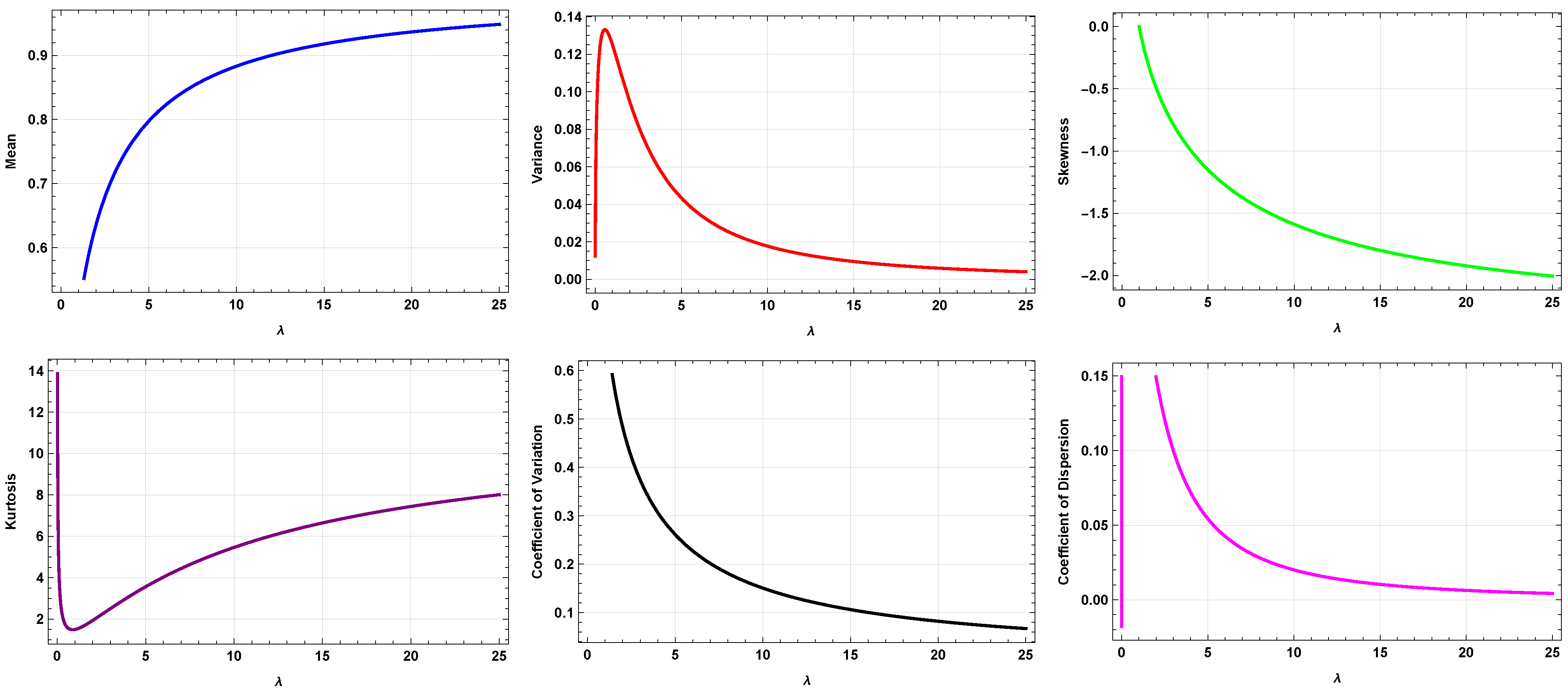
Some numerical values of $Q_1$, $Q_2$, and $Q_3$, as well as the $\mu$, ${\sigma }^2$, ${\gamma }_1$, ${\gamma }_2$, $\mathcal{CV}$, and $\mathcal{CD}$ for various $\lambda$ in the UASED, are summarized in Table 1. The corresponding behavior of these statistical properties as functions of the shape parameter $\lambda$ is illustrated in Figure 3, showing how each property evolves with increasing $\lambda$. The results indicate that, as $\lambda$ increases:

• $Q_1$, $Q_2$, $Q_3$, and $\mu$ increase, while ${\sigma }^2$, $\mathcal{CV}$, and $\mathcal{CD}$ decrease;
• ${\gamma }_1$ decreases from positive to negative values, whereas ${\gamma }_2$ increases;
• Overall, the statistical properties of the UASED vary systematically with $\lambda$.

Table 1. Some numerical values for selected descriptive statistics for the UASED.

$\mathit{\lambda }$	${\mathit{Q}}_1$	${\mathit{Q}}_2$	${\mathit{Q}}_3$	$\mathit{\mu }$	${\mathit{\sigma }}^2$	${\mathit{\gamma }}_1$	${\mathit{\gamma }}_2$	$\mathcal{CV}$	$\mathcal{CD}$
0.01	$3.7\times {10}^{-84}$	$7.9\times {10}^{-31}$	$1.3\times {10}^{-7}$	0.0563	0.0367	3.7200	13.000	3.4000	0.6510
0.26	0.0006	0.0686	0.5420	0.2780	0.1220	0.9420	−0.6820	1.2600	0.4410
0.51	0.0227	0.2550	0.7320	0.3770	0.1330	0.4740	−1.3400	0.9660	0.3520
0.76	0.0788	0.4000	0.8110	0.4470	0.1310	0.1960	−1.5000	0.8090	0.2930
1.00	0.1480	0.5020	0.8540	0.5010	0.1250	−0.0035	−1.5000	0.7050	0.2490
1.30	0.2160	0.5750	0.8810	0.5440	0.1170	−0.1610	−1.4300	0.6290	0.2160
1.50	0.2780	0.6300	0.9000	0.5800	0.1090	−0.2900	−1.3300	0.5700	0.1890
1.80	0.3340	0.6730	0.9140	0.6110	0.1020	−0.4010	−1.2000	0.5230	0.1670
2.00	0.3830	0.7070	0.9240	0.6370	0.0947	−0.4970	−1.0700	0.4830	0.1490
2.50	0.4640	0.7580	0.9390	0.6800	0.0819	−0.6590	−0.7850	0.4210	0.1210
3.60	0.5860	0.8250	0.9570	0.7450	0.0607	−0.9220	−0.1600	0.3310	0.0814
4.70	0.6640	0.8630	0.9670	0.7880	0.0464	−1.1100	0.4190	0.2730	0.0588
5.80	0.7180	0.8870	0.9730	0.8190	0.0365	−1.2500	0.9390	0.2330	0.0445
6.90	0.7570	0.9040	0.9770	0.8420	0.0294	−1.3700	1.4000	0.2040	0.0349
8.00	0.7870	0.9170	0.9800	0.8590	0.0242	−1.4600	1.8200	0.1810	0.0281
9.10	0.8100	0.9270	0.9830	0.8740	0.0202	−1.5400	2.1900	0.1630	0.0232
10.00	0.8280	0.9340	0.9850	0.8850	0.0172	−1.6000	2.5200	0.1480	0.0194
11.00	0.8440	0.9410	0.9860	0.8950	0.0147	−1.6600	2.8200	0.1360	0.0165
12.00	0.8560	0.9460	0.9870	0.9030	0.0128	−1.7100	3.1000	0.1250	0.0142
14.00	0.8670	0.9500	0.9880	0.9100	0.0112	−1.7500	3.3400	0.1160	0.0123
15.00	0.8770	0.9540	0.9890	0.9160	0.0099	−1.7900	3.5700	0.1090	0.0108
16.00	0.8850	0.9570	0.9900	0.9210	0.0088	−1.8200	3.7800	0.1020	0.0096
17.00	0.8920	0.9600	0.9910	0.9260	0.0079	−1.8500	3.9700	0.0960	0.0085
18.00	0.8980	0.9620	0.9910	0.9300	0.0071	−1.8800	4.1400	0.0907	0.0076
19.00	0.9040	0.9640	0.9920	0.9340	0.0064	−1.9000	4.3100	0.0859	0.0069
20.00	0.9060	0.9650	0.9920	0.9350	0.0062	−1.9100	4.3800	0.0839	0.0066
22.00	0.9170	0.9690	0.9930	0.9420	0.0050	−1.9600	4.7100	0.0748	0.0053
25.00	0.9250	0.9720	0.9940	0.9480	0.0041	−2.0000	4.9900	0.0675	0.0043
27.00	0.9320	0.9750	0.9940	0.9530	0.0034	−2.0400	5.2300	0.0615	0.0036
30.00	0.9380	0.9770	0.9950	0.9570	0.0029	−2.0600	5.4400	0.0564	0.0030

Table 1. Some numerical values for selected descriptive statistics for the UASED.

$\mathit{\lambda }$	${\mathit{Q}}_1$	${\mathit{Q}}_2$	${\mathit{Q}}_3$	$\mathit{\mu }$	${\mathit{\sigma }}^2$	${\mathit{\gamma }}_1$	${\mathit{\gamma }}_2$	$\mathcal{CV}$	$\mathcal{CD}$
0.01	$3.7\times {10}^{-84}$	$7.9\times {10}^{-31}$	$1.3\times {10}^{-7}$	0.0563	0.0367	3.7200	13.000	3.4000	0.6510
0.26	0.0006	0.0686	0.5420	0.2780	0.1220	0.9420	−0.6820	1.2600	0.4410
0.51	0.0227	0.2550	0.7320	0.3770	0.1330	0.4740	−1.3400	0.9660	0.3520
0.76	0.0788	0.4000	0.8110	0.4470	0.1310	0.1960	−1.5000	0.8090	0.2930
1.00	0.1480	0.5020	0.8540	0.5010	0.1250	−0.0035	−1.5000	0.7050	0.2490
1.30	0.2160	0.5750	0.8810	0.5440	0.1170	−0.1610	−1.4300	0.6290	0.2160
1.50	0.2780	0.6300	0.9000	0.5800	0.1090	−0.2900	−1.3300	0.5700	0.1890
1.80	0.3340	0.6730	0.9140	0.6110	0.1020	−0.4010	−1.2000	0.5230	0.1670
2.00	0.3830	0.7070	0.9240	0.6370	0.0947	−0.4970	−1.0700	0.4830	0.1490
2.50	0.4640	0.7580	0.9390	0.6800	0.0819	−0.6590	−0.7850	0.4210	0.1210
3.60	0.5860	0.8250	0.9570	0.7450	0.0607	−0.9220	−0.1600	0.3310	0.0814
4.70	0.6640	0.8630	0.9670	0.7880	0.0464	−1.1100	0.4190	0.2730	0.0588
5.80	0.7180	0.8870	0.9730	0.8190	0.0365	−1.2500	0.9390	0.2330	0.0445
6.90	0.7570	0.9040	0.9770	0.8420	0.0294	−1.3700	1.4000	0.2040	0.0349
8.00	0.7870	0.9170	0.9800	0.8590	0.0242	−1.4600	1.8200	0.1810	0.0281
9.10	0.8100	0.9270	0.9830	0.8740	0.0202	−1.5400	2.1900	0.1630	0.0232
10.00	0.8280	0.9340	0.9850	0.8850	0.0172	−1.6000	2.5200	0.1480	0.0194
11.00	0.8440	0.9410	0.9860	0.8950	0.0147	−1.6600	2.8200	0.1360	0.0165
12.00	0.8560	0.9460	0.9870	0.9030	0.0128	−1.7100	3.1000	0.1250	0.0142
14.00	0.8670	0.9500	0.9880	0.9100	0.0112	−1.7500	3.3400	0.1160	0.0123
15.00	0.8770	0.9540	0.9890	0.9160	0.0099	−1.7900	3.5700	0.1090	0.0108
16.00	0.8850	0.9570	0.9900	0.9210	0.0088	−1.8200	3.7800	0.1020	0.0096
17.00	0.8920	0.9600	0.9910	0.9260	0.0079	−1.8500	3.9700	0.0960	0.0085
18.00	0.8980	0.9620	0.9910	0.9300	0.0071	−1.8800	4.1400	0.0907	0.0076
19.00	0.9040	0.9640	0.9920	0.9340	0.0064	−1.9000	4.3100	0.0859	0.0069
20.00	0.9060	0.9650	0.9920	0.9350	0.0062	−1.9100	4.3800	0.0839	0.0066
22.00	0.9170	0.9690	0.9930	0.9420	0.0050	−1.9600	4.7100	0.0748	0.0053
25.00	0.9250	0.9720	0.9940	0.9480	0.0041	−2.0000	4.9900	0.0675	0.0043
27.00	0.9320	0.9750	0.9940	0.9530	0.0034	−2.0400	5.2300	0.0615	0.0036
30.00	0.9380	0.9770	0.9950	0.9570	0.0029	−2.0600	5.4400	0.0564	0.0030

Figure 3. Statistical properties of the UASED as a function of the shape parameter $\lambda$.

Figure 3. Statistical properties of the UASED as a function of the shape parameter $\lambda$.

Theorem 6 (Moment Generating Function of the UASED).

Let $Y\sim \mathrm{UASED}\left(\lambda \right)$ with the PDF given in Equation (4). Then, the moment generating function (MGF) of Y is

$$M_Y\left(t\right)=\mathbb{E}\left[e^{tY}\right]={\displaystyle \frac{1}{\sqrt{\pi }}}\sum _{r=0}^{\infty }{\displaystyle \frac{t^r}{r!}}{\displaystyle \frac{\mathsf{\Gamma }\left(\frac{r}{\lambda }+\frac{1}{2}\right)}{\mathsf{\Gamma }\left(\frac{r}{\lambda }+1\right)}},t\in \mathbb{R}.$$

(11)

Proof. 

By definition, the moment generating function of Y is

$$M_Y\left(t\right)=\mathbb{E}\left[e^{tY}\right]={\int }_0^1{e}^{ty}{f}_Y(y;\lambda )dy.$$

Since $0<Y<1$ almost surely, the MGF exists for all real t. Using the power series expansion of the exponential function,

$$e^{ty}=\sum _{r=0}^{\infty }{\displaystyle \frac{t^r{y}^r}{r!}},$$

which converges absolutely for all $t\in \mathbb{R}$ and $0<y<1$. Substituting this expansion into the integral yields

$$M_Y\left(t\right)={\int }_0^1\sum _{r=0}^{\infty }{\displaystyle \frac{t^r{y}^r}{r!}}{f}_Y(y;\lambda )dy=\sum _{r=0}^{\infty }{\displaystyle \frac{t^r}{r!}}{\int }_0^1{y}^r{f}_Y(y;\lambda )dy=\sum _{r=0}^{\infty }{\displaystyle \frac{t^r}{r!}}{\mu }_r^{\prime }.$$

Substituting the expression for the $r^{th}$ non-central moment from Equation (9), we obtain

$$M_Y\left(t\right)={\displaystyle \frac{1}{\sqrt{\pi }}}\sum _{r=0}^{\infty }{\displaystyle \frac{t^r}{r!}}{\displaystyle \frac{\mathsf{\Gamma }\left(\frac{r}{\lambda }+\frac{1}{2}\right)}{\mathsf{\Gamma }\left(\frac{r}{\lambda }+1\right)}},$$

which completes the proof.    □

Remark 5. 

The $r^{th}$ raw moment can be obtained from the MGF as follows

$${\mu }_r^{\prime }={\left.{\displaystyle \frac{d^r}{d{t}^r}}{M}_Y\left(t\right)\right|}_{t=0},r=1,2,\dots .$$

Theorem 7 (Characteristic Function of the UASED).

Let $Y\sim \mathrm{UASED}\left(\lambda \right)$ with PDF given in Equation (4). Then the characteristic function (CF) of Y is

$${\phi }_Y\left(t\right)=\mathbb{E}\left[e^{itY}\right]=\sum _{r=0}^{\infty }{\displaystyle \frac{{\left(it\right)}^r}{r!}}{\displaystyle \frac{1}{\sqrt{\pi }}}{\displaystyle \frac{\mathsf{\Gamma }\left(\frac{r}{\lambda }+\frac{1}{2}\right)}{\mathsf{\Gamma }\left(\frac{r}{\lambda }+1\right)}},t\in \mathbb{R},\mathit{and}i=\sqrt{-1},$$

(12)

Proof. 

By definition, the characteristic function of Y is

$${\phi }_Y\left(t\right)=\mathbb{E}\left[e^{itY}\right]={\int }_0^1{e}^{ity}{f}_Y(y;\lambda )dy.$$

Since Y is supported on the bounded interval $(0,1)$, the characteristic function exists for all $t\in \mathbb{R}$. Using the power series expansion of the complex exponential,

$$e^{ity}=\sum _{r=0}^{\infty }{\displaystyle \frac{{\left(it\right)}^r{y}^r}{r!}},$$

which converges absolutely for all $t\in \mathbb{R}$ and $0<y<1$. Substituting this expansion into the integral yields

$${\phi }_Y\left(t\right)={\int }_0^1\sum _{r=0}^{\infty }{\displaystyle \frac{{\left(it\right)}^r{y}^r}{r!}}{f}_Y(y;\lambda )dy=\sum _{r=0}^{\infty }{\displaystyle \frac{{\left(it\right)}^r}{r!}}{\int }_0^1{y}^r{f}_Y(y;\lambda )dy=\sum _{r=0}^{\infty }{\displaystyle \frac{{\left(it\right)}^r}{r!}}{\mu }_r^{\prime }.$$

Substituting the expression for the $r^{th}$ non-central moment from Equation (9), we obtain

$${\phi }_Y\left(t\right)={\displaystyle \frac{1}{\sqrt{\pi }}}\sum _{r=0}^{\infty }{\displaystyle \frac{{\left(it\right)}^r}{r!}}{\displaystyle \frac{\mathsf{\Gamma }\left(\frac{r}{\lambda }+\frac{1}{2}\right)}{\mathsf{\Gamma }\left(\frac{r}{\lambda }+1\right)}},$$

which completes the proof.    □

Remark 6. 

The $r^{th}$ raw moment can be obtained from the CF ${\varphi }_Y\left(t\right)$ as follows:

$${\mu }_r^{\prime }={\left.{\displaystyle \frac{1}{i^r}}{\displaystyle \frac{d^r}{d{t}^r}}{\varphi }_Y\left(t\right)\right|}_{t=0},r=1,2,\dots .$$

Definition 1 (Cumulant Generating Function).

The cumulant generating function (CGF) of a random variable Y is defined as

$$K_Y\left(t\right)=log{M}_Y\left(t\right),t\in \mathbb{R},$$

(13)

provided that the MGF $M_Y\left(t\right)$ exists in a neighborhood of the origin. Substituting from Equation (11) into Equation (13), the CGF of the UASED is obtained as

$$K_Y\left(t\right)=log\left[{\displaystyle \frac{1}{\sqrt{\pi }}}\sum _{r=0}^{\infty }{\displaystyle \frac{t^r}{r!}}{\displaystyle \frac{\mathsf{\Gamma }\left(\frac{r}{\lambda }+\frac{1}{2}\right)}{\mathsf{\Gamma }\left(\frac{r}{\lambda }+1\right)}}\right].$$

(14)

Consequently, the $r^{\mathrm{th}}$ cumulant ${\kappa }_r$ of Y is obtained by differentiation of the CGF as

$${\kappa }_r={\left.{\displaystyle \frac{d^r}{d{t}^r}}{K}_Y\left(t\right)\right|}_{t=0},r=1,2,\dots .$$

These cumulants facilitate the systematic derivation of key descriptive measures of the UASED, including $\mu ={\kappa }_1$, ${\sigma }^2={\kappa }_2$, ${\gamma }_1={\kappa }_3/{\kappa }_2^{3/2}$, and ${\gamma }_2={\kappa }_4/{\kappa }_2^2$.

Theorem 8 (Incomplete Moments of the UASED).

Let $Y\sim \mathrm{UASED}\left(\lambda \right)$ with the PDF given in Equation (4). Then, the $r^{th}$ incomplete moment of Y up to $y\in (0,1)$, denoted by ${\psi }_r\left(y\right)$, is expressed as

$${\psi }_r\left(y\right)=\mathbb{E}\left[Y^m{\mathbf{1}}_{\{Y\le y\}}\right]={\int }_0^y{t}^r{f}_Y(t;\lambda )dt={\displaystyle \frac{1}{\pi }}{B}_{y^{\lambda }}\left({\displaystyle \frac{r}{\lambda }}+{\displaystyle \frac{1}{2}},{\displaystyle \frac{1}{2}}\right),0<y<1,r>-{\displaystyle \frac{\lambda }{2}},$$

(15)

where $B_x(a,b)={\int }_0^x{t}^{a-1}{(1-t)}^{b-1}dt$ denotes the incomplete Beta function.

Proof. 

By definition, the $r^{th}$ incomplete moment of Y is

$${\psi }_r\left(y\right)={\int }_0^y{t}^r{f}_Y(t;\lambda )dt={\displaystyle \frac{\lambda }{\pi }}{\int }_0^y{\displaystyle \frac{t^{r+\lambda -1}}{\sqrt{t^{\lambda }(1-t^{\lambda })}}}dt={\displaystyle \frac{\lambda }{\pi }}{\int }_0^y{t}^{r+\frac{\lambda }{2}-1}{(1-t^{\lambda })}^{-\frac{1}{2}}dt.$$

Using the transformation $u=t^{\lambda },dt={\displaystyle \frac{1}{\lambda }}{u}^{\frac{1}{\lambda }-1}du$, the integral becomes

$${\psi }_r\left(y\right)={\displaystyle \frac{1}{\pi }}{\int }_0^{y^{\lambda }}{u}^{\frac{r}{\lambda }-\frac{1}{2}}{(1-u)}^{-\frac{1}{2}}du={\displaystyle \frac{1}{\pi }}{B}_{y^{\lambda }}\left({\displaystyle \frac{r}{\lambda }}+{\displaystyle \frac{1}{2}},{\displaystyle \frac{1}{2}}\right),$$

which completes the proof.    □

Remark 7. 

The incomplete moment ${\psi }_r\left(y\right)$ extends the concept of the standard $r^{\mathrm{th}}$ non-central moment ${\mu }_r^{\prime }$ of the UASED. Specifically, it reduces to the usual non-central moment when $y=1$, i.e., ${\psi }_r\left(1\right)={\mu }_r^{\prime }$, and thus provides a flexible tool for examining the distribution up to any threshold $y\in (0,1)$.

3.4. Mean Residual Life and Mean Inactivity Time

The mean residual life (MRL) and mean inactivity time (MIT) functions are key concepts in reliability theory and survival analysis, quantifying the expected remaining and elapsed lifetimes of a system, respectively. For a random variable $Y\sim \mathrm{UASED}\left(\lambda \right)$ supported on $(0,1)$, the MRL function at $y\in (0,1)$ is defined by

$${\widehat{m}}_r(y;\lambda )=\mathbb{E}[Y-y\mid Y>y]={\displaystyle \frac{1}{R_Y(y;\lambda )}}{\int }_y^{1}t{f}_Y(t;\lambda )dt-y.$$

(16)

By substituting the PDF and RF of the UASED from Equations (4) and (5) into Equation (16), we obtain

$${\widehat{m}}_r(y;\lambda )={\displaystyle \frac{1}{2arcsin\left(\sqrt{1-y^{\lambda }}\right)}}{\int }_y^1{\displaystyle \frac{\lambda t^{\lambda }}{\sqrt{t^{\lambda }(1-t^{\lambda })}}}dt-y.$$

Introducing the transformation $u=t^{\lambda }$, with $dt={\displaystyle \frac{1}{\lambda }}{u}^{\frac{1}{\lambda }-1}du$, we obtain

$${\widehat{m}}_r(y;\lambda )={\displaystyle \frac{1}{2arcsin\left(\sqrt{1-y^{\lambda }}\right)}}{\int }_{y^{\lambda }}^1{u}^{\frac{1}{\lambda }-\frac{1}{2}}{(1-u)}^{-\frac{1}{2}}du.$$

Recognizing the integrand as the standard incomplete Beta function form,

$${\int }_x^1{u}^{a-1}{(1-u)}^{b-1}du=B(a,b)-B_x(a,b),$$

with $a={\displaystyle \frac{1}{\lambda }}+{\displaystyle \frac{1}{2}}$ and $b={\displaystyle \frac{1}{2}}$, we obtain the closed-form representation

$${\widehat{m}}_r(y;\lambda )={\displaystyle \frac{B\left(\frac{1}{\lambda }+\frac{1}{2},\frac{1}{2}\right)-B_{y^{\lambda }}\left(\frac{1}{\lambda }+\frac{1}{2},\frac{1}{2}\right)}{2arcsin\left(\sqrt{1-y^{\lambda }}\right)}}-y.$$

(17)

Similarly, the MIT function at $y\in (0,1)$ is defined by

$${\widehat{m}}_i(y;\lambda )=\mathbb{E}[y-Y\mid Y\le y]={\displaystyle \frac{1}{F_Y(y;\lambda )}}{\int }_0^y{F}_Y(t;\lambda )dt,$$

(18)

By substituting the CDF of the UASED from Equation (3) into Equation (18), we obtain

$${\widehat{m}}_i(y;\lambda )={\displaystyle \frac{1}{1-\frac{2}{\pi }arcsin\left(\sqrt{1-y^{\lambda }}\right)}}{\int }_0^y\left[1-{\displaystyle \frac{2}{\pi }}arcsin\left(\sqrt{1-t^{\lambda }}\right)\right]dt.$$

Using the identity $arcsin\left(x\right)+arcsin\left(\sqrt{1-x^2}\right)={\displaystyle \frac{\pi }{2}}$, we rewrite

$$1-{\displaystyle \frac{2}{\pi }}arcsin\left(\sqrt{1-t^{\lambda }}\right)={\displaystyle \frac{2}{\pi }}arcsin(t^{\frac{\lambda }{2}}),$$

yielding

$$\begin{array}{cc}\hfill {\widehat{m}}_i(y;\lambda )& ={\displaystyle \frac{1}{1-\frac{2}{\pi }arcsin\left(\sqrt{1-y^{\lambda }}\right)}}{\int }_0^y{\displaystyle \frac{2}{\pi }}arcsin(t^{\frac{\lambda }{2}})dt\hfill \\ \hfill & ={\displaystyle \frac{1}{\frac{\pi }{2}-arcsin\left(\sqrt{1-y^{\lambda }}\right)}}{\int }_0^{y}arcsin(t^{\frac{\lambda }{2}})dt.\hfill \end{array}$$

Applying the substitution $u=t^{\lambda }$, $dt={\displaystyle \frac{1}{\lambda }}{u}^{\frac{1}{\lambda }-1}du$ gives

$${\widehat{m}}_i(y;\lambda )={\displaystyle \frac{1}{\frac{\pi }{2}-arcsin\left(\sqrt{1-y^{\lambda }}\right)}}\left[{\displaystyle \frac{1}{\lambda }}{\int }_0^{y^{\lambda }}arcsin\left(\sqrt{u}\right)u^{\frac{1}{\lambda }-1}du\right].$$

Using integration by parts with $v=arcsin\left(\sqrt{u}\right)$ and $dw=u^{\frac{1}{\lambda }-1}du$, we obtain

$${\widehat{m}}_i(y;\lambda )={\displaystyle \frac{1}{\frac{\pi }{2}-arcsin\left(\sqrt{1-y^{\lambda }}\right)}}\left[yarcsin(y^{\frac{\lambda }{2}})-{\displaystyle \frac{1}{2}}{\int }_0^{y^{\lambda }}{u}^{\frac{1}{\lambda }-\frac{1}{2}}{(1-u)}^{-\frac{1}{2}}du\right].$$

Recognizing the remaining integral as an incomplete Beta function $B_x(a,b)$ with $a={\displaystyle \frac{1}{\lambda }}+{\displaystyle \frac{1}{2}}$ and $b={\displaystyle \frac{1}{2}}$, the MIT function can be expressed in closed form as

$$\begin{array}{cc}\hfill {\widehat{m}}_i(y;\lambda )& ={\displaystyle \frac{1}{\frac{\pi }{2}-arcsin\left(\sqrt{1-y^{\lambda }}\right)}}\left[yarcsin\left(y^{\frac{\lambda }{2}}\right)-{\displaystyle \frac{1}{2}}{B}_{y^{\lambda }}\left({\displaystyle \frac{1}{\lambda }}+{\displaystyle \frac{1}{2}},{\displaystyle \frac{1}{2}}\right)\right].\hfill \end{array}$$

(19)

3.5. Order Statistics

Order statistics play a crucial role in many areas of statistical theory and applications, particularly in survival analysis and quality control. In this subsection, we present the order statistics of the proposed UASED. Let $Y_{1:n}\le Y_{2:n}\le \cdots \le Y_{n:n}$ denote the order statistics of a random sample of size n drawn from $Y\sim \mathrm{UASED}\left(\lambda \right)$. The PDF of the $r^{th}$ order statistic, $r=1,2,\dots ,n$, is given by

$$f_{Y_{r:n}}(y;\lambda )={\displaystyle \frac{n!}{(r-1)!(n-r)!}}{\left[F_Y(y;\lambda )\right]}^{r-1}{[1-F_Y(y;\lambda )]}^{n-r}{f}_Y(y;\lambda ),$$

and its corresponding CDF is given by

$$F_{Y_{r:n}}(y;\lambda )=\sum _{k=r}^n\sum _{m=0}^{n-k}\left({\displaystyle \genfrac{}{}{0pt}{}{n}{k}}\right)\left({\displaystyle \genfrac{}{}{0pt}{}{n-k}{m}}\right){(-1)}^m{\left[F_Y(y;\lambda )\right]}^{m+k}.$$

Substituting the CDF and PDF of the UASED from Equations (3) and (4), respectively, yields

$$\begin{array}{cc}\hfill f_{Y_{r:n}}(y;\lambda )& ={\displaystyle \frac{n!}{(r-1)!(n-r)!}}{\left[1-{\displaystyle \frac{2}{\pi }}arcsin\left(\sqrt{1-y^{\lambda }}\right)\right]}^{r-1}{\left[{\displaystyle \frac{2}{\pi }}arcsin\left(\sqrt{1-y^{\lambda }}\right)\right]}^{n-r}\hfill \\ \hfill & \times {\displaystyle \frac{\lambda y^{\lambda -1}}{\pi \sqrt{y^{\lambda }(1-y^{\lambda })}}},\hfill \end{array}$$

(20)

and

$$F_{Y_{r:n}}(y;\lambda )=\sum _{k=r}^n\sum _{m=0}^{n-k}\left({\displaystyle \genfrac{}{}{0pt}{}{n}{k}}\right)\left({\displaystyle \genfrac{}{}{0pt}{}{n-k}{m}}\right){(-1)}^m{\left[1-{\displaystyle \frac{2}{\pi }}arcsin\left(\sqrt{1-y^{\lambda }}\right)\right]}^{m+k}.$$

(21)

In particular, the first (minimum) and last (maximum) order statistics correspond to $r=1$ and $r=n$, respectively. Their PDFs are given explicitly as follows:

• Minimum: $Y_{1:n}$

  $$f_{Y_{1:n}}(y;\lambda )=n{\left[{\displaystyle \frac{2}{\pi }}arcsin\left(\sqrt{1-y^{\lambda }}\right)\right]}^{n-1}{\displaystyle \frac{\lambda y^{\lambda -1}}{\pi \sqrt{y^{\lambda }(1-y^{\lambda })}}},0<y<1,$$
• Maximum: $Y_{n:n}$

  $$f_{Y_{n:n}}(y;\lambda )=n{\left[1-{\displaystyle \frac{2}{\pi }}arcsin\left(\sqrt{1-y^{\lambda }}\right)\right]}^{n-1}{\displaystyle \frac{\lambda y^{\lambda -1}}{\pi \sqrt{y^{\lambda }(1-y^{\lambda })}}},0<y<1.$$

3.6. Entropy Measures

Entropy provides a quantitative measure of uncertainty and information content associated with a probability distribution and plays a central role in information theory, reliability analysis, and risk assessment. For the UASED, several generalized entropy measures can be derived in closed form by evaluating a common integral involving the PDF. Let $Y\sim \mathrm{UASED}\left(\lambda \right)$ with PDF given in Equation (4). For $\delta >0$, $\delta \ne 1$, consider the integral

$$I_{\delta }\left(\lambda \right)={\int }_0^1{\left[f_Y(y;\lambda )\right]}^{\delta }dy.$$

(22)

Substituting the PDF and simplifying yields

$$I_{\delta }\left(\lambda \right)={\displaystyle \frac{{\lambda }^{\delta }}{{\pi }^{\delta }}}{\int }_0^1{y}^{\delta (\lambda -1)-\frac{\delta \lambda }{2}}{(1-y^{\lambda })}^{-\frac{\delta }{2}}dy={\displaystyle \frac{{\lambda }^{\delta }}{{\pi }^{\delta }}}{\int }_0^1{y}^{\frac{\delta \lambda }{2}-\delta }{(1-y^{\lambda })}^{-\frac{\delta }{2}}dy.$$

Applying the transformation $t=y^{\lambda }$, with $dy={\displaystyle \frac{1}{\lambda }}{t}^{\frac{1}{\lambda }-1}dt$, the integral becomes

$$I_{\delta }\left(\lambda \right)={\displaystyle \frac{{\lambda }^{\delta -1}}{{\pi }^{\delta }}}{\int }_0^1{t}^{\frac{\delta }{2}-\frac{\delta }{\lambda }+\frac{1}{\lambda }-1}{(1-t)}^{-\frac{\delta }{2}}dt.$$

Recognizing this as a Beta integral, we obtain

$$I_{\delta }\left(\lambda \right)={\displaystyle \frac{{\lambda }^{\delta -1}}{{\pi }^{\delta }}}B\left({\displaystyle \frac{2+\delta (\lambda -2)}{2\lambda }},1-{\displaystyle \frac{\delta }{2}}\right),0<\delta <2,\delta \ne 1.$$

Using the identity $B(a,b)={\displaystyle \frac{\mathsf{\Gamma }\left(a\right)\mathsf{\Gamma }\left(b\right)}{\mathsf{\Gamma }(a+b)}}$, the integral admits the closed-form expression

$$I_{\delta }\left(\lambda \right)={\displaystyle \frac{{\lambda }^{\delta -1}}{{\pi }^{\delta }}}{\displaystyle \frac{\mathsf{\Gamma }\left(\frac{2+\delta (\lambda -2)}{2\lambda }\right)\mathsf{\Gamma }\left(1-\frac{\delta }{2}\right)}{\mathsf{\Gamma }\left(\frac{\lambda +1-\delta }{\lambda }\right)}},0<\delta <2,\delta \ne 1.$$

(23)

All generalized entropy measures considered below follow directly from $I_{\delta }\left(\lambda \right)$ in Equation (23).

3.6.1. Rényi Entropy

The Rényi ($\mathcal{R}$) entropy [11] of order $\delta$ is defined as

$$\begin{array}{cc}\hfill {\mathcal{R}}_{\delta }\left(\lambda \right)& ={\displaystyle \frac{1}{1-\delta }}log\left[I_{\delta }\left(\lambda \right)\right]\hfill \\ \hfill & ={\displaystyle \frac{1}{1-\delta }}log\left[{\displaystyle \frac{{\lambda }^{\delta -1}}{{\pi }^{\delta }}}{\displaystyle \frac{\mathsf{\Gamma }\left(\frac{2+\delta (\lambda -2)}{2\lambda }\right)\mathsf{\Gamma }\left(1-\frac{\delta }{2}\right)}{\mathsf{\Gamma }\left(\frac{\lambda +1-\delta }{\lambda }\right)}}\right],0<\delta <2,\delta \ne 1.\hfill \end{array}$$

(24)

3.6.2. Arimoto Entropy

The Arimoto ($\mathcal{A}$) entropy [12] of order $\delta$ is defined by

$$\begin{array}{cc}\hfill {\mathcal{A}}_{\delta }\left(\lambda \right)& ={\displaystyle \frac{\delta }{1-\delta }}\left[I_{\delta }{\left(\lambda \right)}^{\frac{1}{\delta }}-1\right]\hfill \\ \hfill & ={\displaystyle \frac{\delta }{1-\delta }}\left[{\left({\displaystyle \frac{{\lambda }^{\delta -1}}{{\pi }^{\delta }}}{\displaystyle \frac{\mathsf{\Gamma }\left(\frac{2+\delta (\lambda -2)}{2\lambda }\right)\mathsf{\Gamma }\left(1-\frac{\delta }{2}\right)}{\mathsf{\Gamma }\left(\frac{\lambda +1-\delta }{\lambda }\right)}}\right)}^{\frac{1}{\delta }}-1\right],0<\delta <2,\delta \ne 1.\hfill \end{array}$$

(25)

3.6.3. Tsallis Entropy

The Tsallis ($\mathcal{T}$) entropy [13,14] of order $\delta$ is given by

$$\begin{array}{cc}\hfill {\mathcal{T}}_{\delta }\left(\lambda \right)& ={\displaystyle \frac{1}{\delta -1}}\left[1-I_{\delta }\left(\lambda \right)\right]\hfill \\ \hfill & ={\displaystyle \frac{1}{\delta -1}}\left[1-{\displaystyle \frac{{\lambda }^{\delta -1}}{{\pi }^{\delta }}}{\displaystyle \frac{\mathsf{\Gamma }\left(\frac{2+\delta (\lambda -2)}{2\lambda }\right)\mathsf{\Gamma }\left(1-\frac{\delta }{2}\right)}{\mathsf{\Gamma }\left(\frac{\lambda +1-\delta }{\lambda }\right)}}\right],0<\delta <2,\delta \ne 1.\hfill \end{array}$$

(26)

3.6.4. Havrda–Charvát Entropy

The Havrda–Charvát ($\mathcal{HC}$) entropy [15] of order $\delta$ is defined as

$$\begin{array}{cc}\hfill {\mathcal{HC}}_{\delta }\left(\lambda \right)& ={\displaystyle \frac{1}{2^{1-\delta }-1}}\left[I_{\delta }\left(\lambda \right)-1\right]\hfill \\ \hfill & ={\displaystyle \frac{1}{2^{1-\delta }-1}}\left[{\displaystyle \frac{{\lambda }^{\delta -1}}{{\pi }^{\delta }}}{\displaystyle \frac{\mathsf{\Gamma }\left(\frac{2+\delta (\lambda -2)}{2\lambda }\right)\mathsf{\Gamma }\left(1-\frac{\delta }{2}\right)}{\mathsf{\Gamma }\left(\frac{\lambda +1-\delta }{\lambda }\right)}}-1\right],0<\delta <2,\delta \ne 1.\hfill \end{array}$$

(27)

3.6.5. Mathai–Haubold Entropy

The Mathai–Haubold ($\mathcal{MH}$) entropy [16] of order $\delta$ is defined as

$$\begin{array}{cc}\hfill {\mathcal{MH}}_{\delta }\left(\lambda \right)& ={\displaystyle \frac{1}{\delta -1}}\left[I_{(2-\delta )}\left(\lambda \right)-1\right]\hfill \\ \hfill & ={\displaystyle \frac{1}{\delta -1}}\left[{\displaystyle \frac{{\lambda }^{1-\delta }}{{\pi }^{2-\delta }}}{\displaystyle \frac{\mathsf{\Gamma }\left(1-\frac{\delta }{2}+\frac{\delta -1}{\lambda }\right)\mathsf{\Gamma }\left(\frac{\delta }{2}\right)}{\mathsf{\Gamma }\left(\frac{\lambda +\delta -1}{\lambda }\right)}}-1\right],0<\delta <2,\delta \ne 1.\hfill \end{array}$$

(28)

3.6.6. Shannon Entropy

Shannon (${\mathcal{S}}_h$) entropy [17] is another classical measure of entropy for continuous random variables. For a random variable Y with PDF $f_Y(y;\lambda )$, it is defined as

$${\mathcal{S}}_h\left(\lambda \right)=-\mathbb{E}\left[log{f}_Y(Y;\lambda )\right].$$

Let $Y\sim \mathrm{UASED}\left(\lambda \right)$ with the PDF given in Equation (4). Substituting $f_Y(y;\lambda )$ into the definition yields   

$${\mathcal{S}}_h\left(\lambda \right)=-\mathbb{E}\left[log\left({\displaystyle \frac{\lambda y^{\lambda -1}}{\pi \sqrt{y^{\lambda }(1-y^{\lambda })}}}\right)\right]=-log\left({\displaystyle \frac{\lambda }{\pi }}\right)-{\displaystyle \frac{\lambda -2}{2}}\mathbb{E}[logY]+{\displaystyle \frac{1}{2}}\mathbb{E}\left[log(1-Y^{\lambda })\right].$$

By applying the transformation $t=y^{\lambda }$ and leveraging the standard Beta–digamma integrals

$${\int }_0^1{t}^{a-1}{(1-t)}^{b-1}logtdt=B(a,b)\left[\psi \left(a\right)-\psi (a+b)\right],$$

$${\int }_0^1{t}^{a-1}{(1-t)}^{b-1}log(1-t)dt=B(a,b)\left[\psi \left(b\right)-\psi (a+b)\right],$$

where $B(a,b)$ denotes the Beta function and $\psi (·)$ is the digamma function, defined by

$$\psi \left(x\right)={\displaystyle \frac{d}{dx}}log\mathsf{\Gamma }\left(x\right)={\displaystyle \frac{{\mathsf{\Gamma }}^{\prime }\left(x\right)}{\mathsf{\Gamma }\left(x\right)}},x>0,$$

one can show that

$$\mathbb{E}[logY]=-{\displaystyle \frac{log4}{\lambda }},\mathbb{E}\left[log(1-Y^{\lambda })\right]=-log4.$$

Consequently, the Shannon entropy of the UASED is

$${\mathcal{S}}_h\left(\lambda \right)=-log\left({\displaystyle \frac{\lambda }{\pi }}\right)-{\displaystyle \frac{log4}{\lambda }},\lambda >0.$$

(29)

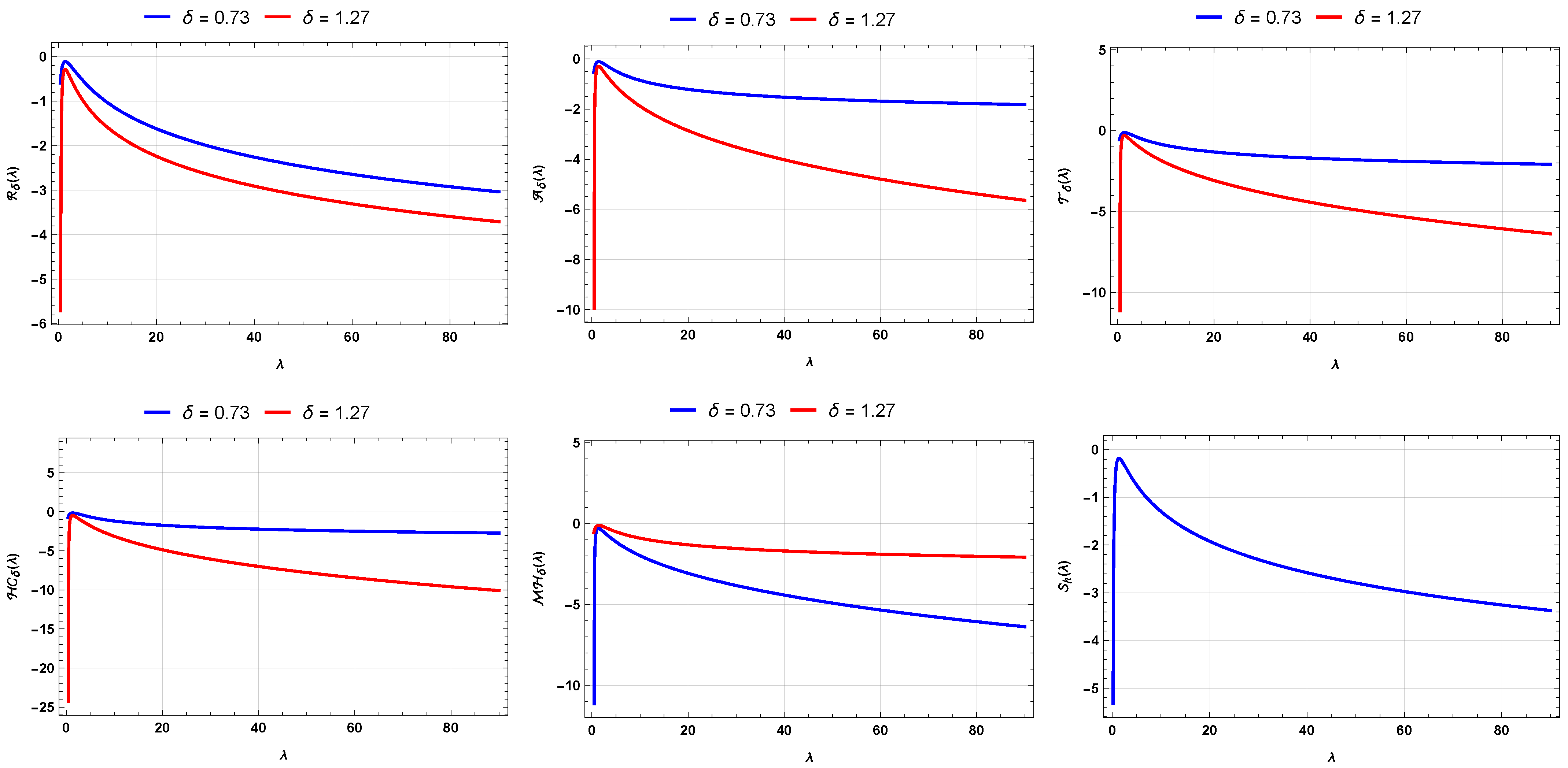
The entropy measures are flexible in characterizing the UASED under various parametric conditions and have been used in reliability modeling, information theory, and statistical inferences. Numerical values of the selected entropy measure for $\delta =0.73$ and $\delta =1.27$ are presented in Table 2 and the plots in Figure 4. The results indicate that:

• For a fixed value of $\delta$, all entropy measures, ${\mathcal{R}}_{\delta }\left(\lambda \right)$, ${\mathcal{A}}_{\delta }\left(\lambda \right)$, ${\mathcal{T}}_{\delta }\left(\lambda \right)$, ${\mathcal{HC}}_{\delta }\left(\lambda \right)$, and ${\mathcal{MH}}_{\delta }\left(\lambda \right)$ decrease as $\lambda$ increases, reflecting reduced uncertainty;
• For fixed $\lambda$, entropy values at $\delta =1.27$ are lower than at $\delta =0.73$, indicating greater sensitivity of higher-order $\delta$ to distributional concentration;
• ${\mathcal{S}}_h\left(\lambda \right)$ depends solely on $\lambda$ and decreases monotonically as $\lambda$ increases;
• Overall, the UASED offers flexible modeling of uncertainty across different measures and parameter settings.

Figure 4. Plots of selected entropy measures for the UASED at $\delta =0.73$ and $\delta =1.27$.

Figure 4. Plots of selected entropy measures for the UASED at $\delta =0.73$ and $\delta =1.27$.

Table 2. Some numerical values of entropy measures for the UASED at $\delta =0.73$ and $\delta =1.27$.

$\mathit{\lambda }$	$\mathit{\delta }$	${\mathcal{R}}_{\mathit{\delta }}\left(\mathit{\lambda }\right)$	${\mathcal{A}}_{\mathit{\delta }}\left(\mathit{\lambda }\right)$	${\mathcal{T}}_{\mathit{\delta }}\left(\mathit{\lambda }\right)$	${\mathcal{HC}}_{\mathit{\delta }}\left(\mathit{\lambda }\right)$	${\mathcal{MH}}_{\mathit{\delta }}\left(\mathit{\lambda }\right)$	${\mathcal{S}}_{\mathit{h}}\left(\mathit{\lambda }\right)$
0.05	0.73	−2.8623	−1.7657	−1.9936	−2.6155	2.9706	−23.5854
	1.27	5.9990	3.3899	2.9706	4.6991	−1.9936
0.70	0.73	−0.2657	−0.2531	−0.2564	−0.3364	−1.0776	−0.4790
	1.27	−0.9458	−1.0476	−1.0776	−1.7046	−0.2564
1.35	0.73	−0.1125	−0.1102	−0.1108	−0.1454	−0.2983	−0.1823
	1.27	−0.2869	−0.2958	−0.2983	−0.4719	−0.1108
2.00	0.73	−0.1486	−0.1446	−0.1457	−0.1911	−0.4007	−0.2416
	1.27	−0.3805	−0.3963	−0.4007	−0.6339	−0.1457
2.50	0.73	−0.2079	−0.2001	−0.2022	−0.2652	−0.5279	−0.3261
	1.27	−0.4935	−0.5203	−0.5279	−0.8350	−0.2022
6.63	0.73	−0.7240	−0.6351	−0.6576	−0.8627	−1.4480	−0.9554
	1.27	−1.2222	−1.3957	−1.4480	−2.2906	−0.6576
10.80	0.73	−1.0891	−0.8965	−0.9436	−1.2379	−2.0852	−1.3591
	1.27	−1.6541	−1.9822	−2.0852	−3.2986	−0.9436
14.90	0.73	−1.3592	−1.0683	−1.1377	−1.4926	−2.5771	−1.6481
	1.27	−1.9562	−2.4257	−2.5771	−4.0768	−1.1377
19.00	0.73	−1.5726	−1.1924	−1.2813	−1.6810	−2.9833	−1.8727
	1.27	−2.1882	−2.7863	−2.9833	−4.7192	−1.2813
19.50	0.73	−1.5956	−1.2052	−1.2964	−1.7007	−3.0282	−1.8968
	1.27	−2.2131	−2.8259	−3.0282	−4.7903	−1.2964
21.60	0.73	−1.6871	−1.2550	−1.3551	−1.7777	−3.2086	−1.9921
	1.27	−2.3110	−2.9844	−3.2086	−5.0758	−1.3551
23.70	0.73	−1.7709	−1.2993	−1.4077	−1.8467	−3.3772	−2.0792
	1.27	−2.4003	−3.1316	−3.3772	−5.3425	−1.4077
25.80	0.73	−1.8483	−1.3389	−1.4551	−1.9090	−3.5356	−2.1594
	1.27	−2.4822	−3.2693	−3.5356	−5.5930	−1.4551
27.90	0.73	−1.9201	−1.3747	−1.4983	−1.9657	−3.6852	−2.2336
	1.27	−2.5580	−3.3988	−3.6852	−5.8297	−1.4983
30.00	0.73	−1.9872	−1.4073	−1.5379	−2.0176	−3.8270	−2.3027
	1.27	−2.6284	−3.5210	−3.8270	−6.0540	−1.5379

Table 2. Some numerical values of entropy measures for the UASED at $\delta =0.73$ and $\delta =1.27$.

$\mathit{\lambda }$	$\mathit{\delta }$	${\mathcal{R}}_{\mathit{\delta }}\left(\mathit{\lambda }\right)$	${\mathcal{A}}_{\mathit{\delta }}\left(\mathit{\lambda }\right)$	${\mathcal{T}}_{\mathit{\delta }}\left(\mathit{\lambda }\right)$	${\mathcal{HC}}_{\mathit{\delta }}\left(\mathit{\lambda }\right)$	${\mathcal{MH}}_{\mathit{\delta }}\left(\mathit{\lambda }\right)$	${\mathcal{S}}_{\mathit{h}}\left(\mathit{\lambda }\right)$
0.05	0.73	−2.8623	−1.7657	−1.9936	−2.6155	2.9706	−23.5854
	1.27	5.9990	3.3899	2.9706	4.6991	−1.9936
0.70	0.73	−0.2657	−0.2531	−0.2564	−0.3364	−1.0776	−0.4790
	1.27	−0.9458	−1.0476	−1.0776	−1.7046	−0.2564
1.35	0.73	−0.1125	−0.1102	−0.1108	−0.1454	−0.2983	−0.1823
	1.27	−0.2869	−0.2958	−0.2983	−0.4719	−0.1108
2.00	0.73	−0.1486	−0.1446	−0.1457	−0.1911	−0.4007	−0.2416
	1.27	−0.3805	−0.3963	−0.4007	−0.6339	−0.1457
2.50	0.73	−0.2079	−0.2001	−0.2022	−0.2652	−0.5279	−0.3261
	1.27	−0.4935	−0.5203	−0.5279	−0.8350	−0.2022
6.63	0.73	−0.7240	−0.6351	−0.6576	−0.8627	−1.4480	−0.9554
	1.27	−1.2222	−1.3957	−1.4480	−2.2906	−0.6576
10.80	0.73	−1.0891	−0.8965	−0.9436	−1.2379	−2.0852	−1.3591
	1.27	−1.6541	−1.9822	−2.0852	−3.2986	−0.9436
14.90	0.73	−1.3592	−1.0683	−1.1377	−1.4926	−2.5771	−1.6481
	1.27	−1.9562	−2.4257	−2.5771	−4.0768	−1.1377
19.00	0.73	−1.5726	−1.1924	−1.2813	−1.6810	−2.9833	−1.8727
	1.27	−2.1882	−2.7863	−2.9833	−4.7192	−1.2813
19.50	0.73	−1.5956	−1.2052	−1.2964	−1.7007	−3.0282	−1.8968
	1.27	−2.2131	−2.8259	−3.0282	−4.7903	−1.2964
21.60	0.73	−1.6871	−1.2550	−1.3551	−1.7777	−3.2086	−1.9921
	1.27	−2.3110	−2.9844	−3.2086	−5.0758	−1.3551
23.70	0.73	−1.7709	−1.2993	−1.4077	−1.8467	−3.3772	−2.0792
	1.27	−2.4003	−3.1316	−3.3772	−5.3425	−1.4077
25.80	0.73	−1.8483	−1.3389	−1.4551	−1.9090	−3.5356	−2.1594
	1.27	−2.4822	−3.2693	−3.5356	−5.5930	−1.4551
27.90	0.73	−1.9201	−1.3747	−1.4983	−1.9657	−3.6852	−2.2336
	1.27	−2.5580	−3.3988	−3.6852	−5.8297	−1.4983
30.00	0.73	−1.9872	−1.4073	−1.5379	−2.0176	−3.8270	−2.3027
	1.27	−2.6284	−3.5210	−3.8270	−6.0540	−1.5379

3.7. Stress-Strength Reliability

Stress–strength reliability (SSR) measures the probability that a system’s strength exceeds the applied stress. Let $Y_1$ and $Y_2$ denote the system strength and applied stress, respectively, with $Y_1\sim \mathrm{UASED}\left({\lambda }_1\right)$ and $Y_2\sim \mathrm{UASED}\left({\lambda }_2\right)$, where ${\lambda }_1,{\lambda }_2>0$, and assume that $Y_1$ and $Y_2$ are independent. Then, the system operates successfully if $Y_1>Y_2$, and the SSR is given by

$${\mathcal{R}}_{ss}=\mathbb{P}(Y_1>Y_2)={\int }_0^1{f}_{Y_1}(y;{\lambda }_1)F_{Y_2}(y;{\lambda }_2)dy.$$

(30)

Using the CDF and PDF of the UASED given in Equations (3) and (4), we obtain

$$\begin{array}{cc}\hfill {\mathcal{R}}_{ss}& ={\int }_0^1\left[1-{\displaystyle \frac{2}{\pi }}arcsin\left(\sqrt{1-y^{{\lambda }_2}}\right)\right]{\displaystyle \frac{{\lambda }_1{y}^{{\lambda }_1-1}}{\pi \sqrt{y^{{\lambda }_1}(1-y^{{\lambda }_1})}}}dy\hfill \\ \hfill & =1-{\displaystyle \frac{2}{{\pi }^2}}{\int }_0^{1}arcsin\left(\sqrt{1-y^{{\lambda }_2}}\right){\displaystyle \frac{{\lambda }_1{y}^{{\lambda }_1-1}}{\sqrt{y^{{\lambda }_1}(1-y^{{\lambda }_1})}}}dy.\hfill \end{array}$$

Applying the transformation $t=y^{{\lambda }_1}$, $dt={\lambda }_1{y}^{{\lambda }_1-1}dy$, yields

$${\mathcal{R}}_{ss}=1-{\displaystyle \frac{2}{{\pi }^2}}{\int }_0^1{\displaystyle \frac{arcsin\left(\sqrt{1-t^{\alpha }}\right)}{\sqrt{t(1-t)}}}dt,\alpha ={\displaystyle \frac{{\lambda }_2}{{\lambda }_1}}.$$

(31)

To evaluate the integral, consider the substitution $t={sin}^{2}x$, $x\in [0,{\displaystyle \frac{\pi }{2}}]$, giving $dt=2sinxcosxdx$ and $\sqrt{t(1-t)}=cosx$. Then,

$$I_{\alpha }={\int }_0^1{\displaystyle \frac{arcsin\left(\sqrt{1-t^{\alpha }}\right)}{\sqrt{t(1-t)}}}dt=2{\int }_0^{\frac{\pi }{2}}arcsin\left(\sqrt{1-{sin}^{2\alpha }x}\right)dx.$$

Using the identity $arcsin\left(\sqrt{1-z}\right)={\displaystyle \frac{\pi }{2}}-arcsin\left(\sqrt{z}\right)$, we further simplify

$$I_{\alpha }=2{\int }_0^{\frac{\pi }{2}}\left[{\displaystyle \frac{\pi }{2}}-arcsin\left({sin}^{\alpha }x\right)\right]dx={\displaystyle \frac{{\pi }^2}{2}}-2{\int }_0^{\frac{\pi }{2}}arcsin\left({sin}^{\alpha }x\right)dx.$$

Expanding $arcsin\left(u\right)$ via its Taylor series,

$$arcsin\left(u\right)=\sum _{k=0}^{\infty }{\displaystyle \frac{\left(2k\right)!}{4^k{(k!)}^2(2k+1)}}{u}^{2k+1},\left|u\right|\le 1,$$

we obtain

$$\begin{array}{cc}\hfill I_{\alpha }& ={\displaystyle \frac{{\pi }^2}{2}}-2{\int }_0^{\frac{\pi }{2}}\sum _{k=0}^{\infty }{\displaystyle \frac{\left(2k\right)!}{4^k{(k!)}^2(2k+1)}}{\left({sin}^{\alpha }x\right)}^{2k+1}dx\hfill \\ \hfill & ={\displaystyle \frac{{\pi }^2}{2}}-2\sum _{k=0}^{\infty }{\displaystyle \frac{\left(2k\right)!}{4^k{(k!)}^2(2k+1)}}{\int }_0^{\frac{\pi }{2}}{\left(sinx\right)}^{\alpha (2k+1)}dx.\hfill \end{array}$$

It is well-known that the integral of a power of the sine function over $[0,{\displaystyle \frac{\pi }{2}}]$ can be expressed in terms of the Beta function $B(x,y)={\displaystyle \frac{\mathsf{\Gamma }\left(x\right)\mathsf{\Gamma }\left(y\right)}{\mathsf{\Gamma }(x+y)}}$:

$${\int }_0^{\frac{\pi }{2}}{sin}^m\theta d\theta ={\displaystyle \frac{1}{2}}B\left({\displaystyle \frac{m+1}{2}},{\displaystyle \frac{1}{2}}\right)={\displaystyle \frac{\sqrt{\pi }}{2}}{\displaystyle \frac{\mathsf{\Gamma }\left(\frac{m+1}{2}\right)}{\mathsf{\Gamma }\left(\frac{m+2}{2}\right)}},m>-1.$$

Thus, the series representation of $I_{\alpha }$ is

$$I_{\alpha }={\displaystyle \frac{{\pi }^2}{2}}-\sqrt{\pi }\sum _{k=0}^{\infty }{\displaystyle \frac{\left(2k\right)!}{4^k{(k!)}^2(2k+1)}}{\displaystyle \frac{\mathsf{\Gamma }\left(\frac{\alpha (2k+1)+1}{2}\right)}{\mathsf{\Gamma }\left(\frac{\alpha (2k+1)+2}{2}\right)}}.$$

(32)

Finally, substituting the result of Equation (32), into Equation (31), the SSR of the UASED is

$$\begin{array}{cc}\hfill {\mathcal{R}}_{ss}& =1-{\displaystyle \frac{2}{{\pi }^2}}\left[{\displaystyle \frac{{\pi }^2}{2}}-\sqrt{\pi }\sum _{k=0}^{\infty }{\displaystyle \frac{\left(2k\right)!}{4^k{(k!)}^2(2k+1)}}{\displaystyle \frac{\mathsf{\Gamma }\left(\frac{\alpha (2k+1)+1}{2}\right)}{\mathsf{\Gamma }\left(\frac{\alpha (2k+1)+2}{2}\right)}}\right]\hfill \\ \hfill & ={\displaystyle \frac{2}{{\pi }^{\frac{3}{2}}}}\sum _{k=0}^{\infty }{\displaystyle \frac{\left(2k\right)!}{4^k{(k!)}^2(2k+1)}}{\displaystyle \frac{\mathsf{\Gamma }\left(\frac{\alpha (2k+1)+1}{2}\right)}{\mathsf{\Gamma }\left(\frac{\alpha (2k+1)+2}{2}\right)}},\alpha >0.\hfill \end{array}$$

(33)

Remark 8 (Convergence and truncation error in SSR).

Let

$$a_k\left(\alpha \right)={\displaystyle \frac{\left(2k\right)!}{4^k{(k!)}^2(2k+1)}}{\displaystyle \frac{\mathsf{\Gamma }\left(\frac{\alpha (2k+1)+1}{2}\right)}{\mathsf{\Gamma }\left(\frac{\alpha (2k+1)+2}{2}\right)}},\alpha >0,$$

so that the SSR in Equation (33) can be expressed as ${\mathcal{R}}_{ss}={\displaystyle \frac{2}{{\pi }^{\frac{3}{2}}}}{\displaystyle \sum _{k=0}^{\infty }}{a}_k\left(\alpha \right).$ To investigate the convergence of this representation, we analyze the asymptotic behavior of the summand $a_k\left(\alpha \right)$ as $k\to \infty$. By Stirling’s approximation for factorials given in [18],

$$k!\sim \sqrt{2\pi k}{\left({\displaystyle \frac{k}{e}}\right)}^k\mathit{and}\mathsf{\Gamma }\left(k\right)\sim \sqrt{2\pi }{k}^{k-\frac{1}{2}}{e}^{-k},k\to \infty ,$$

the central binomial factor satisfies

$${\displaystyle \frac{\left(2k\right)!}{4^k{(k!)}^2}}\sim {\left(\pi k\right)}^{-1/2},k\to \infty .$$

Moreover, for large z, the ratio of Gamma functions obeys the well-known asymptotic relation

$${\displaystyle \frac{\mathsf{\Gamma }(z+a)}{\mathsf{\Gamma }(z+b)}}\sim z^{a-b},z\to \infty .$$

Setting $z={\displaystyle \frac{\alpha (2k+1)+1}{2}}$ yields $z\sim \alpha k$ as $k\to \infty$, and therefore

$${\displaystyle \frac{\mathsf{\Gamma }\left(\frac{\alpha (2k+1)+1}{2}\right)}{\mathsf{\Gamma }\left(\frac{\alpha (2k+1)+2}{2}\right)}}\sim {\left(\alpha k\right)}^{-1/2}.$$

Combining these asymptotic relations with the factor ${(2k+1)}^{-1}\sim {\left(2k\right)}^{-1}$ gives

$$a_k\left(\alpha \right)\sim {\displaystyle \frac{1}{\sqrt{\pi k}}}·{\displaystyle \frac{1}{2k}}·{\displaystyle \frac{1}{\sqrt{\alpha k}}}={\displaystyle \frac{1}{2\sqrt{\pi \alpha }}}{k}^{-2},k\to \infty .$$

Hence, the summand decays at the same rate as the terms of a p-series with exponent $p=2$. Since ${\displaystyle \sum _{k=1}^{\infty }}{k}^{-2}$ is convergent, it follows by comparison that the series representation of ${\mathcal{R}}_{ss}$ is absolutely convergent for all $\alpha >0$. Let $S_J\left(\alpha \right)={\displaystyle \frac{2}{{\pi }^{\frac{3}{2}}}}{\displaystyle \sum _{k=0}^J}{a}_k\left(\alpha \right)={\displaystyle \frac{1}{{\pi }^2\sqrt{\alpha }}}{\displaystyle \sum _{k=0}^J}{k}^{-2}$ denote the partial sum obtained by truncating the series after J terms, and define the truncation error by

$$E_J\left(\alpha \right)={\mathcal{R}}_{ss}-S_J\left(\alpha \right)={\displaystyle \frac{2}{{\pi }^{\frac{3}{2}}}}{\displaystyle \sum _{k=J+1}^{\infty }}{a}_k\left(\alpha \right).$$

Since $a_k\left(\alpha \right)$ is positive and asymptotically proportional to $k^{-2}$, the tail of the series behaves like the remainder of the p-series $\sum k^{-2}$. Using the classical integral bound

$${\displaystyle \sum _{k=J+1}^{\infty }}{k}^{-2}\le {\int }_J^{\infty }{x}^{-2}dx={\displaystyle \frac{1}{J}},$$

we obtain

$$E_J\left(\alpha \right)=O\left(J^{-1}\right),J\to \infty .$$

A sharper asymptotic estimate follows from the known expansion of the tail of $\sum k^{-2}$, giving

$$E_J\left(\alpha \right)\sim {\displaystyle \frac{1}{{\pi }^2\sqrt{\alpha }}}{\displaystyle \frac{1}{J}},J\to \infty .$$

Therefore, the series representation in Equation (33) converges absolutely, and the truncation error decreases at the rate $J^{-1}$, indicating that accurate numerical values of the SSR can be obtained using a moderate number of terms.

4. Non-Bayesian Inference

This section addresses the estimation of the parameter $\lambda$ for the UASED, as well as the associated functions $R_Y(y;\lambda )$ and $h_Y(y;\lambda )$, using classical (non-Bayesian) inference methods. The classical methods are categorized into likelihood-based and spacing-based techniques. Asymptotic confidence intervals (ACIs) are also provided.

4.1. Maximum Likelihood Estimation

Let $y_1,y_2,\dots ,y_n$ be a random sample of size n drawn from the UASED with parameter $\lambda >0$ and PDF $f_Y(y;\lambda )$ given in Equation (4). The likelihood function corresponding to this sample is

$$\mathcal{L}\left(\lambda \right)=\prod _{i=1}^n{f}_Y(y_i;\lambda )=\prod _{i=1}^n{\displaystyle \frac{\lambda y_i^{\lambda -1}}{\pi \sqrt{y_i^{\lambda }\left(1-y_i^{\lambda }\right)}}},0<y_i<1.$$

(34)

Taking the natural logarithm of $\mathcal{L}\left(\lambda \right)$ yields the log-likelihood function as

$${\ell }_{\mathrm{ML}}\left(\lambda \right)=nlog\left({\displaystyle \frac{\lambda }{\pi }}\right)+\left({\displaystyle \frac{\lambda }{2}}-1\right)\sum _{i=1}^{n}log{y}_i-{\displaystyle \frac{1}{2}}\sum _{i=1}^{n}log\left(1-y_i^{\lambda }\right).$$

(35)

Then, the maximum likelihood (ML) estimator of the parameter $\lambda$, denoted by ${\widehat{\lambda }}_{\mathrm{ML}}$, is obtained by maximizing ${\ell }_{\mathrm{ML}}\left(\lambda \right)$ in Equation (35). Specifically, ${\widehat{\lambda }}_{\mathrm{ML}}=arg\underset{\lambda >0}{max}{\ell }_{\mathrm{ML}}\left(\lambda \right)$. Differentiating ${\ell }_{\mathrm{ML}}\left(\lambda \right)$ with respect to $\lambda$ and setting it equal to zero leads to the score equation:

$${\displaystyle \frac{\partial {\ell }_{\mathrm{ML}}\left(\lambda \right)}{\partial \lambda }}={\displaystyle \frac{n}{\lambda }}+{\displaystyle \frac{1}{2}}\sum _{i=1}^{n}log{y}_i+{\displaystyle \frac{1}{2}}\sum _{i=1}^n\left({\displaystyle \frac{y_i^{\lambda }log{y}_i}{1-y_i^{\lambda }}}\right)=0.$$

(36)

4.2. Maximum Product of Spacings Estimation

The maximum product of spacings (MPS) method is another suitable choice for estimating parameters by maximizing the average of the spacings or, in simpler terms, the sum of their logarithms. This approach possesses favorable asymptotic properties for a broad class of continuous distributions [19]. Since the proposed UASED satisfies the necessary regularity conditions, specifically a smooth CDF and an identifiable parameter $\lambda$ as established in Theorem 1, these general asymptotic results, including consistency and normality, are directly applicable to the present model. Let $y_{1:n}<y_{2:n}<\cdots <y_{n:n}$ denote an ordered sample of size n drawn from the UASED with parameter $\lambda >0$ and CDF $F_Y(·;\lambda )$ given in Equation (3). The product of spacings function corresponding to this sample is

$$\mathcal{P}\left(\lambda \right)={\left\{\prod _{i=1}^{n+1}{\mathcal{D}}_i\left(\lambda \right)\right\}}^{{\displaystyle \frac{1}{n+1}}},{\mathcal{D}}_i\left(\lambda \right)=\left\{\begin{array}{cc}{F}_Y\left(y_{1:n};\lambda \right),\hfill & i=1,\hfill \\ F_Y\left(y_{i:n};\lambda \right)-F_Y\left(y_{(i-1):n};\lambda \right),\hfill & i=2,\dots ,n,\hfill \\ 1-F_Y\left(y_{n:n};\lambda \right),\hfill & i=n+1,\hfill \end{array}\right.$$

(37)

where ${\mathcal{D}}_i\left(\lambda \right)$ represent the spacings and satisfy ${\displaystyle \sum _{i=1}^{n+1}}{\mathcal{D}}_i\left(\lambda \right)=1$. Explicitly, we have

$$\begin{array}{cc}\hfill \mathcal{P}\left(\lambda \right)=& \{\left[1-{\displaystyle \frac{2}{\pi }}arcsin\left(\sqrt{1-y_{1:n}^{\lambda }}\right)\right]\times \left[{\displaystyle \frac{2}{\pi }}arcsin\left(\sqrt{1-y_{n:n}^{\lambda }}\right)\right]\hfill \\ & \times \prod _{i=2}^n{\displaystyle \frac{2}{\pi }}\left[arcsin\left(\sqrt{1-y_{(i-1):n}^{\lambda }}\right)-arcsin\left(\sqrt{1-y_{i:n}^{\lambda }}\right)\right]{\}}^{{\displaystyle \frac{1}{n+1}}}.\hfill \end{array}$$

(38)

Accordingly, taking the natural logarithm of $\mathcal{P}\left(\lambda \right)$ yields the log product of spacings function as

$$\begin{array}{cc}\hfill {\ell }_{\mathrm{MPS}}\left(\lambda \right)& ={\displaystyle \frac{1}{n+1}}\{log\left[1-{\displaystyle \frac{2}{\pi }}arcsin\left(\sqrt{1-y_{1:n}^{\lambda }}\right)\right]+log\left[{\displaystyle \frac{2}{\pi }}arcsin\left(\sqrt{1-y_{n:n}^{\lambda }}\right)\right]\hfill \\ \hfill & +(n-1)log{\displaystyle \frac{2}{\pi }}+\sum _{i=2}^{n}log\left[arcsin\left(\sqrt{1-y_{(i-1):n}^{\lambda }}\right)-arcsin\left(\sqrt{1-y_{i:n}^{\lambda }}\right)\right]\}.\hfill \end{array}$$

(39)

Then, the MPS estimator of the parameter $\lambda$, denoted by ${\widehat{\lambda }}_{\mathrm{MPS}}$, is obtained by maximizing ${\ell }_{\mathrm{MPS}}\left(\lambda \right)$ in Equation (39). Specifically, ${\widehat{\lambda }}_{\mathrm{MPS}}=arg\underset{\lambda >0}{max}{\ell }_{\mathrm{MPS}}\left(\lambda \right)$. Differentiating ${\ell }_{\mathrm{MPS}}\left(\lambda \right)$ with respect to $\lambda$ and setting it equal to zero leads to the following score equation:

$$\begin{array}{cc}\hfill {\displaystyle \frac{\partial {\ell }_{\mathrm{MPS}}\left(\lambda \right)}{\partial \lambda }}={\displaystyle \frac{1}{n+1}}& \{{\displaystyle \frac{{\displaystyle \frac{1}{\pi }\frac{\sqrt{y_{1:n}^{\lambda }}log{y}_{1:n}}{\sqrt{1-y_{1:n}^{\lambda }}}}}{{\displaystyle 1-\frac{2}{\pi }arcsin\left(\sqrt{1-y_{1:n}^{\lambda }}\right)}}}-{\displaystyle \frac{{\displaystyle \frac{\sqrt{y_{n:n}^{\lambda }}log{y}_{n:n}}{2\sqrt{1-y_{n:n}^{\lambda }}}}}{{\displaystyle arcsin\left(\sqrt{1-y_{n:n}^{\lambda }}\right)}}}\hfill \\ \hfill & +\sum _{i=2}^n{\displaystyle \frac{{\displaystyle \frac{\sqrt{y_{i:n}^{\lambda }}log{y}_{i:n}}{2\sqrt{1-y_{i:n}^{\lambda }}}-\frac{\sqrt{y_{(i-1):n}^{\lambda }}log{y}_{(i-1):n}}{2\sqrt{1-y_{(i-1):n}^{\lambda }}}}}{{\displaystyle arcsin\left(\sqrt{1-y_{(i-1):n}^{\lambda }}\right)-arcsin\left(\sqrt{1-y_{i:n}^{\lambda }}\right)}}}\}=0.\hfill \end{array}$$

(40)

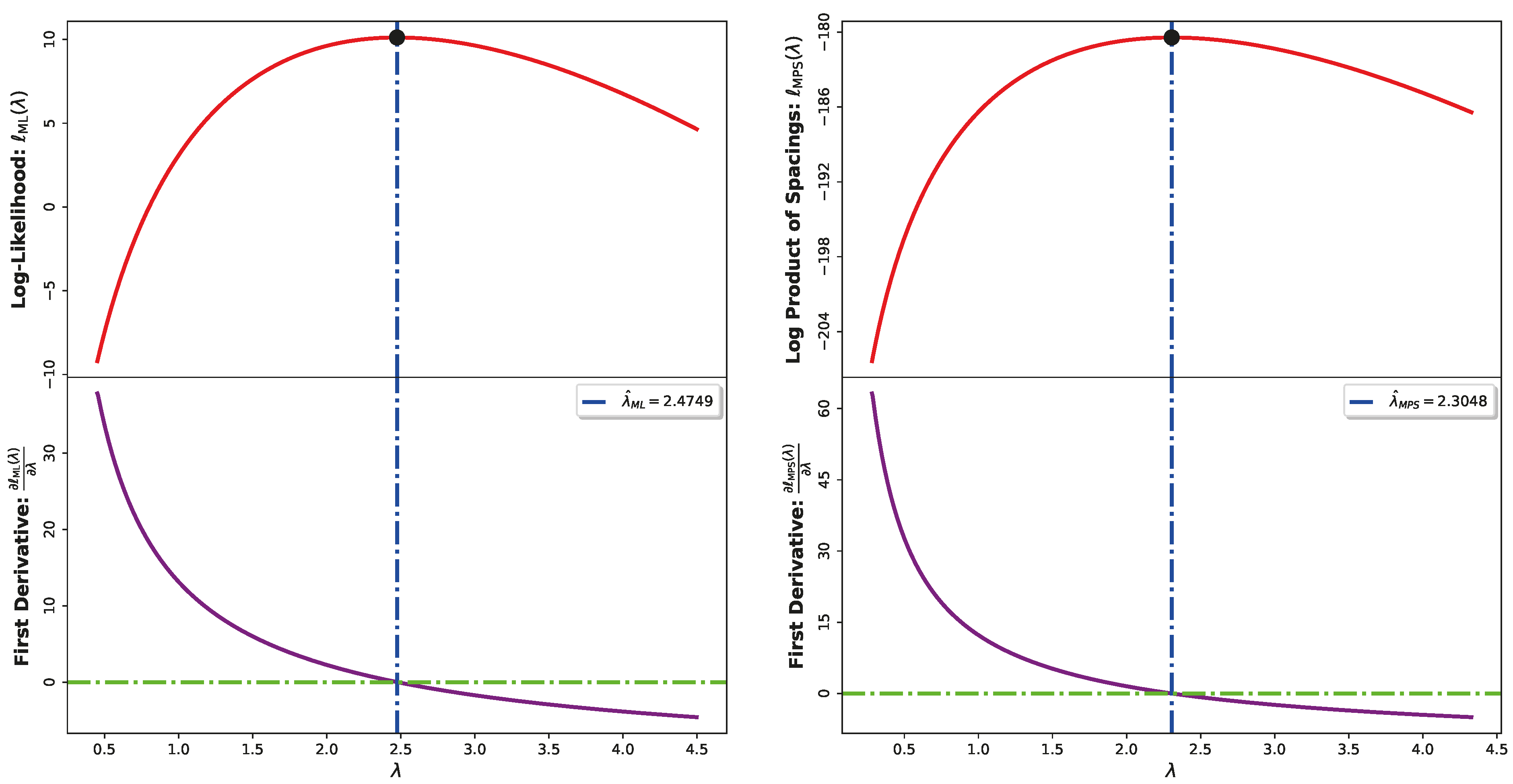
Since Equations (36) and (40) do not admit closed-form solutions, the maximization of ${\ell }_{\mathrm{ML}}\left(\lambda \right)$ and ${\ell }_{\mathrm{MPS}}\left(\lambda \right)$ is carried out numerically using the L-BFGS-B algorithm in Python’s SciPy library [20]. Although nonlinear, the objective functions are smooth and locally concave for $\lambda >0$, and the numerical results in Figure 5 suggest unimodality, ensuring convergence to a unique global maximum.

The corresponding estimators of $R_Y(y;\lambda )$ and $h_Y(y;\lambda )$ are then derived by substituting ${\widehat{\lambda }}_{\mathrm{ML}}$ or ${\widehat{\lambda }}_{\mathrm{MPS}}$ into Equations (5) and (6), respectively, in accordance with the invariance property of ML and MPS estimators [21,22].

4.3. Asymptotic Confidence Intervals

Under the standard regularity conditions, the ML estimator ${\widehat{\lambda }}_{\mathrm{ML}}$ is asymptotically normally distributed about the true parameter value $\lambda$, i.e., ${\widehat{\lambda }}_{\mathrm{ML}}-\lambda \stackrel{d}{\to }\mathcal{N}\left(0,{\mathcal{I}}^{-1}\left(\lambda \right)\right)$, where $\mathcal{N}(·)$ denotes the normal distribution and ${\mathcal{I}}^{-1}(·)$ represents the variance–covariance matrix of the UASED parameter obtained from the Fisher information matrix (FIM) for $\lambda$, defined as $\mathcal{I}\left(\lambda \right)=-\mathbf{E}\left[{\displaystyle \frac{{\partial }^2{\ell }_{\mathrm{ML}}\left(\lambda \right)}{\partial {\lambda }^2}}\right]$. Since the expectation in the FIM may not admit a closed-form expression, the observed FIM evaluated at the ML estimator is commonly used:

$$\widehat{\mathcal{I}}\left({\widehat{\lambda }}_{\mathrm{ML}}\right)=-{\displaystyle \frac{{\partial }^2{\ell }_{\mathrm{ML}}\left(\lambda \right)}{\partial {\lambda }^2}}{|}_{\lambda ={\widehat{\lambda }}_{\mathrm{ML}}}.$$

(41)

Consequently, the asymptotic variance of ${\widehat{\lambda }}_{\mathrm{ML}}$ is estimated as $\widehat{\mathrm{Var}}\left({\widehat{\lambda }}_{\mathrm{ML}}\right)={\widehat{\mathcal{I}}}^{-1}\left({\widehat{\lambda }}_{\mathrm{ML}}\right)$, and a $100(1-\gamma )\%$ two-sided ACI for $\lambda$ is given by

$${\widehat{\lambda }}_{\mathrm{ML}}\pm z_{\frac{\gamma }{2}}\sqrt{\widehat{\mathrm{Var}}\left({\widehat{\lambda }}_{\mathrm{ML}}\right)},$$

where $z_{\frac{\gamma }{2}}$ denotes the upper ${\displaystyle \frac{\gamma }{2}}$ quantile of the standard normal distribution. For functions of $\lambda$, such as $R_Y(y;\lambda )$ and $h_Y(y;\lambda )$, the delta method [23] is employed to approximate the corresponding asymptotic variances:

$$\widehat{\mathrm{Var}}\left(R_Y(y;{\widehat{\lambda }}_{\mathrm{ML}})\right)={\left[{\displaystyle \frac{\partial R_Y(y;\lambda )}{\partial \lambda }}{|}_{\lambda ={\widehat{\lambda }}_{\mathrm{ML}}}\right]}^2\widehat{\mathrm{Var}}\left({\widehat{\lambda }}_{\mathrm{ML}}\right)$$

and

$$\widehat{\mathrm{Var}}\left(h_Y(y;{\widehat{\lambda }}_{\mathrm{ML}})\right)={\left[{\displaystyle \frac{\partial h_Y(y;\lambda )}{\partial \lambda }}{|}_{\lambda ={\widehat{\lambda }}_{\mathrm{ML}}}\right]}^2\widehat{\mathrm{Var}}\left({\widehat{\lambda }}_{\mathrm{ML}}\right).$$

Accordingly, the $100(1-\gamma )\%$ ACIs for $R_Y(y;\lambda )$ and $h_Y(y;\lambda )$ are

$$R_Y(y;{\widehat{\lambda }}_{\mathrm{ML}})\pm z_{\frac{\gamma }{2}}\sqrt{\widehat{\mathrm{Var}}\left(R_Y(y;{\widehat{\lambda }}_{\mathrm{ML}})\right)}\mathrm{and}{h}_Y(y;{\widehat{\lambda }}_{\mathrm{ML}})\pm z_{\frac{\gamma }{2}}\sqrt{\widehat{\mathrm{Var}}\left(h_Y(y;{\widehat{\lambda }}_{\mathrm{ML}})\right)}.$$

Analogously, the ACIs for the MPS estimator ${\widehat{\lambda }}_{\mathrm{MPS}}$ and its corresponding functions $R_Y(y;{\widehat{\lambda }}_{\mathrm{MPS}})$ and $h_Y(y;{\widehat{\lambda }}_{\mathrm{MPS}})$ are obtained by replacing ${\widehat{\lambda }}_{\mathrm{ML}}$ with ${\widehat{\lambda }}_{\mathrm{MPS}}$ and using the corresponding observed information from ${\ell }_{\mathrm{MPS}}\left(\lambda \right)$. These ACIs provide a rigorous measure of uncertainty associated with the parameter estimates and their corresponding functions under both the ML and MPS frameworks [21,22,23].

5. Bayesian Inference

In this section, Bayesian methods are employed to estimate the UASED parameter $\lambda$, along with its associated functions $R_Y(y;\lambda )$ and $h_Y(y;\lambda )$. Within the Bayesian paradigm, $\lambda$ is regarded as a random variable endowed with a prior distribution. Two prior specifications are considered: an informative Gamma prior and the non-informative Jeffreys’ prior. Specifically, we assume a Gamma prior for $\lambda$ with density

$$\mathcal{G}\left(\lambda \right)\propto {\lambda }^{a_1-1}{e}^{-b_1\lambda },a_1>0,b_1>0,\lambda >0,$$

(42)

where $a_1$ and $b_1$ are hyperparameters. For the informative prior, $(a_1,b_1)$ are chosen by moment matching, equating the prior mean and variance to the empirical moments of ${\widehat{\lambda }}_{\mathrm{ML}}$ (or ${\widehat{\lambda }}_{\mathrm{MPS}}$) [24]. When prior information is unavailable, we adopt Jeffreys’ prior, $\mathcal{G}\left(\lambda \right)\propto {\lambda }^{-1}$, which corresponds to the limiting case $a_1=b_1=0$.

5.1. Bayesian Estimation Under ML

Let $y_1,y_2,\dots ,y_n$ denote a random sample of size n from the UASED with parameter $\lambda >0$, and let $\mathbf{y}=(y_1,\dots ,y_n)$. Combining the prior density in Equation (42) with the likelihood function in Equation (34) yields the posterior density of $\lambda$, up to a normalizing constant, as

$${\mathcal{G}}_{\mathrm{ML}}^{*}(\lambda \mid \mathbf{y})={\displaystyle \frac{\mathcal{G}\left(\lambda \right)\mathcal{L}\left(\lambda \right)}{\underset{0}{\overset{\infty }{\int }}\mathcal{G}\left(\lambda \right)\mathcal{L}\left(\lambda \right)d\lambda }}\propto {\lambda }^{a_1}{e}^{-b_1\lambda }\prod _{i=1}^n{\displaystyle \frac{y_i^{\lambda -1}}{\sqrt{y_i^{\lambda }\left(1-y_i^{\lambda }\right)}}}.$$

(43)

5.2. Bayesian Inference Under MPS

An alternative Bayesian estimation procedure is developed under the MPS framework. Let $y_{1:n}<y_{2:n}<\cdots <y_{n:n}$ denote an ordered sample of size n from the UASED with parameter $\lambda >0$, and let $\mathbf{y}=(y_{1:n},\dots ,y_{n:n})$. Combining the prior density in Equation (42) with the product-of-spacings function in Equation (38) yields the posterior density of $\lambda$, up to a normalizing constant, as

$$\begin{array}{cc}\hfill {\mathcal{G}}_{\mathrm{MPS}}^{*}(\lambda \mid \mathbf{y})& ={\displaystyle \frac{\mathcal{G}\left(\lambda \right)\mathcal{P}\left(\lambda \right)}{{\int }_0^{\infty }\mathcal{G}\left(\lambda \right)\mathcal{P}\left(\lambda \right)d\lambda }}\propto {\lambda }^{a_1-1}{e}^{-b_1\lambda }\{\left[1-{\displaystyle \frac{2}{\pi }}arcsin\left(\sqrt{1-y_{1:n}^{\lambda }}\right)\right]\hfill \\ \hfill & \times \left[arcsin\left(\sqrt{1-y_{n:n}^{\lambda }}\right)\right]\prod _{i=2}^n\left[arcsin\left(\sqrt{1-y_{(i-1):n}^{\lambda }}\right)-arcsin\left(\sqrt{1-y_{i:n}^{\lambda }}\right)\right]{\}}^{{\displaystyle \frac{1}{n+1}}}.\hfill \end{array}$$

(44)

Bayesian estimation of the UASED parameter $\lambda$ and the associated functions $R_Y(y;\lambda )$ and $h_Y(y;\lambda )$ is conducted under the symmetric squared error loss (SEL) function, $L(\lambda ,\widehat{\lambda })={(\widehat{\lambda }-\lambda )}^2$. Under SEL, the Bayes estimator of any function $g\left(\lambda \right)$ is its posterior mean,

$${\widehat{g}}_{\mathrm{SEL}}\left(\lambda \right)=\mathbf{E}\left[g\left(\lambda \right)\mid \mathbf{y}\right]=\underset{0}{\overset{\infty }{\int }}g\left(\lambda \right){\mathcal{G}}^{*}(\lambda \mid \mathbf{y})d\lambda .$$

(45)

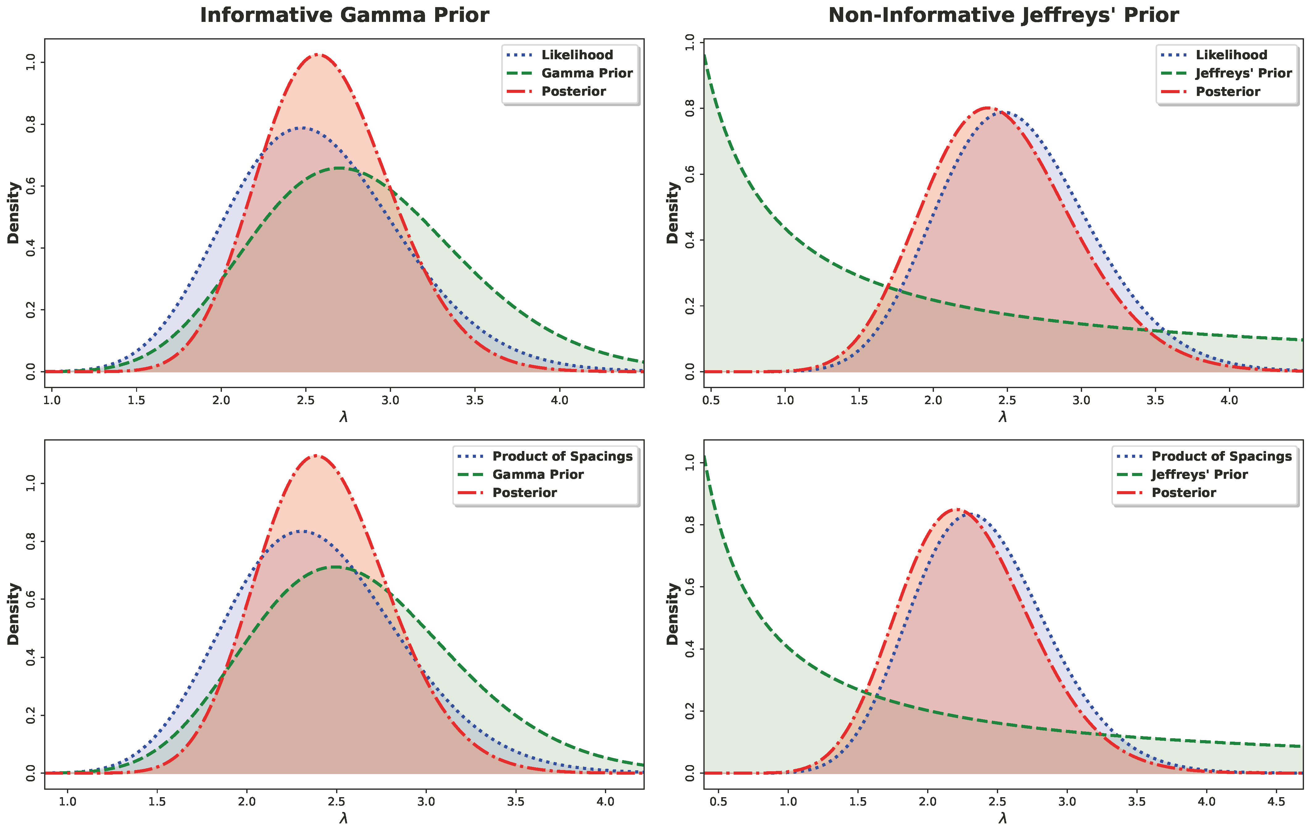
Here, ${\mathcal{G}}^{*}(\lambda \mid \mathbf{y})$ denotes the posterior density, which equals ${\mathcal{G}}_{\mathrm{ML}}^{*}(\lambda \mid \mathbf{y})$ under the ML-based approach or ${\mathcal{G}}_{\mathrm{MPS}}^{*}(\lambda \mid \mathbf{y})$ under the MPS-based approach. Because the posterior distributions in Equations (43) and (44) do not belong to a standard family and are not available in closed form, posterior moments and Bayesian estimates cannot be evaluated analytically. Accordingly, we use Markov chain Monte Carlo (MCMC) methods and employ the Metropolis–Hastings (M–H) algorithm to generate samples from ${\mathcal{G}}_{\mathrm{ML}}^{*}(\lambda \mid \mathbf{y})$ or ${\mathcal{G}}_{\mathrm{MPS}}^{*}(\lambda \mid \mathbf{y})$. The M–H algorithm is particularly effective here because the posterior distributions are close to normal, as shown in Figure 6, which allows for the use of symmetric normal proposal distributions.

Moreover, the acceptance probability ensures convergence to the target posterior [25,26,27]. Based on these samples, we compute Bayesian point estimates and report corresponding highest posterior density (HPD) credible intervals (CRIs). The M–H procedure within Gibbs sampling is implemented as follows:

• Input: Starting value ${\lambda }^{\left(0\right)}=\widehat{\lambda }$, proposal variance $\widehat{\mathrm{Var}}\left(\widehat{\lambda }\right)$, total number of iterations ${\mathcal{M}}^{•}$, burn-in size ${\mathcal{M}}_0$, confidence level $(1-\gamma )$, and posterior density ${\mathcal{G}}^{*}(\lambda \mid \mathbf{y})$.
• Set the iterator to $\kappa \leftarrow 1$.
• Repeat for $\kappa =1,\dots ,{\mathcal{M}}^{•}$:

  (a)

  Propose a new candidate value ${\lambda }^{*}\sim \mathcal{N}\left({\lambda }^{(\kappa -1)},\widehat{\mathrm{Var}}\left(\widehat{\lambda }\right)\right),{\lambda }^{*}>0;$

  (b)

  Evaluate the acceptance probability $\mathsf{\Omega }=min\left(1,{\displaystyle \frac{{\mathcal{G}}^{*}({\lambda }^{*}\mid \mathbf{y})}{{\mathcal{G}}^{*}({\lambda }^{(\kappa -1)}\mid \mathbf{y})}}\right);$

  (c)

  Draw $u\sim \mathcal{U}(0,1)$;

  (d)

  Accept the proposal if $u\le \mathsf{\Omega }$ by setting ${\lambda }^{\left(\kappa \right)}\leftarrow {\lambda }^{*}$; otherwise, keep the previous state, i.e., ${\lambda }^{\left(\kappa \right)}\leftarrow {\lambda }^{(\kappa -1)}$;

  (e)

  Evaluate $R_Y(y;\lambda )$ and $h_Y(y;\lambda )$ by substituting ${\lambda }^{\left(\kappa \right)}$ for $\lambda$;

  (f)

  Increment the iterator: $\kappa \leftarrow \kappa +1$.

• Discard the first ${\mathcal{M}}_0$ values (burn-in) and keep $\{{\lambda }^{({\mathcal{M}}_0+1)},\dots ,{\lambda }^{\left(\mathcal{M}\right)}\}.$
• Obtain the Bayes estimator under SEL as ${\tilde{\lambda }}_{\mathrm{SEL}}={\displaystyle \frac{1}{{\mathcal{M}}^{*}}}{\displaystyle \sum _{\kappa ={\mathcal{M}}_0+1}^{\mathcal{M}}}{\lambda }^{\left(\kappa \right)},{\mathcal{M}}^{*}={\mathcal{M}}^{•}-{\mathcal{M}}_0.$
• Form the $(1-\gamma )100\%$ HPD CRI as follows:

  (a)

  Arrange the retained values in ascending order as ${\lambda }_{\left(1\right)}\le \cdots \le {\lambda }_{\left({\mathcal{M}}^{*}\right)};$

  (b)

  For $\kappa =1,\dots ,\gamma {\mathcal{M}}^{*}$, calculate $\delta \left(\kappa \right)={\lambda }_{(\kappa +(1-\gamma ){\mathcal{M}}^{*})}-{\lambda }_{\left(\kappa \right)};$

  (c)

  Define ${\kappa }^{*}=arg{min}_{\kappa }\delta \left(\kappa \right)$;

  (d)

  The corresponding HPD CRI is $\left({\lambda }_{\left({\kappa }^{*}\right)},{\lambda }_{({\kappa }^{*}+(1-\gamma ){\mathcal{M}}^{*})}\right).$

• Repeat Steps (5) and (6) for $R_Y(y;\lambda )$ and $h_Y(y;\lambda )$.

6. Monte Carlo Simulation Study

This section presents a Monte Carlo simulation study to evaluate the statistical efficiency of the UASED model. The analysis focuses on point and interval inference for the parameter $\lambda$ and the associated functions $R_Y(y,\lambda )$ and $h_Y(y,\lambda )$, evaluated at the fixed time point $y=0.5$.

6.1. Simulation Design

To examine estimator performance under varying conditions, several combinations of sample sizes and parameter values are considered. For each configuration, ${\mathcal{M}}_g=1000$ independent samples are generated from the UASED distribution using the inverse transform method in Equation (8). The simulation settings are:

• Sample Sizes: $n=20,40,80,160,320,$ and 640;
• True Parameter Values: $\lambda =0.30,0.90,2.70,8.10,$ and $13.50$.

A comparative framework is adopted to study the performance of the ML and MPS estimators, together with their Bayesian counterparts. Classical estimation and the construction of $90\%$ and $95\%$ ACIs are implemented using the L-BFGS-B algorithm available in Python’s SciPy library [20]. Bayesian inference is conducted under informative Gamma priors, with hyperparameters $({\mu }_1,{\nu }_1)$ specified for each $(n,\lambda )$ configuration, and non-informative Jeffreys’ priors to assess prior sensitivity. Posterior summaries under the SEL function, including $90\%$ and $95\%$ HPD CRIs, are obtained via the M–H algorithm described in Section 5. The MCMC procedure is run for ${\mathcal{M}}^{•}=12,000$ iterations, with the first ${\mathcal{M}}_0=2000$ iterations discarded as burn-in. The accuracy of the point estimators $\widehat{\varphi }$, where $\varphi \in \{\lambda ,R_Y(y,\lambda ),h_Y(y,\lambda )\}$, is evaluated using:

• Average Estimate (AE): $\mathrm{AE}\left(\widehat{\varphi }\right)={\displaystyle \frac{1}{{\mathcal{M}}_g}}{\displaystyle \sum _{i=1}^{{\mathcal{M}}_g}}{\widehat{\varphi }}_{\left(i\right)},$ where ${\widehat{\varphi }}_{\left(i\right)}$ denotes the estimate obtained from the ith simulated dataset;
• Root Mean Squared Error (RMSE): $\mathrm{RMSE}\left(\widehat{\varphi }\right)=\sqrt{{\displaystyle \frac{1}{{\mathcal{M}}_g}}{\displaystyle \sum _{i=1}^{{\mathcal{M}}_g}}{({\widehat{\varphi }}_{\left(i\right)}-\varphi )}^2}$;
• Mean Relative Absolute Bias (MRAB): $\mathrm{MRAB}\left(\widehat{\varphi }\right)={\displaystyle \frac{1}{{\mathcal{M}}_g}}{\displaystyle \sum _{i=1}^{{\mathcal{M}}_g}}{\displaystyle \frac{|{\widehat{\varphi }}_{\left(i\right)}-\varphi |}{\varphi }}.$

Interval estimation is assessed using the $90\%$ and $95\%$ ACIs and HPD CRIs through:

• Average Length (AL): ${\mathrm{AL}}_{100(1-\gamma )\%}\left(\widehat{\varphi }\right)={\displaystyle \frac{1}{{\mathcal{M}}_g}}{\displaystyle \sum _{i=1}^{{\mathcal{M}}_g}}\left(U_{{\widehat{\varphi }}_{\left(i\right)}}-L_{{\widehat{\varphi }}_{\left(i\right)}}\right),$ where $\gamma \in \{0.05,0.10\}$ and $L_{{\widehat{\varphi }}_{\left(i\right)}}$ and $U_{{\widehat{\varphi }}_{\left(i\right)}}$ denote the lower and upper bounds, respectively;
• Coverage Probability (CP): ${\mathrm{CP}}_{100(1-\gamma )\%}\left(\widehat{\varphi }\right)={\displaystyle \frac{1}{{\mathcal{M}}_g}}{\displaystyle \sum _{i=1}^{{\mathcal{M}}_g}}{\mathcal{I}}_{\left[L_{{\widehat{\varphi }}_{\left(i\right)}},U_{{\widehat{\varphi }}_{\left(i\right)}}\right]}\left(\varphi \right),$ where $\mathcal{I}(·)$ is the indicator function.

6.2. Simulation Algorithm

The simulation procedure is implemented in Python 3.10. using the autograd and scipy.optimize libraries and proceeds as follows:

Step 1: 

Specify the true value of $\lambda$ and the sample size n;

Step 2: 

Generate n observations from $U(0,1)$ and transform them into UASED samples using $Q_Y(u;\lambda )$;

Step 3: 

Get the solution of the numerical optimization of ${\widehat{\lambda }}_{ML}$ or ${\widehat{\lambda }}_{MPS}$;

Step 4: 

Run the MCMC chains under informative and non-informative priors with a normal proposal distribution;

Step 5: 

Calculate the AE, RMSE, MRAB, AL, and CP Values of each quantity;

Step 6: 

Repeat the procedure ${\mathcal{M}}_g$ times to arrive at aggregate outcomes.

6.3. Simulation Results

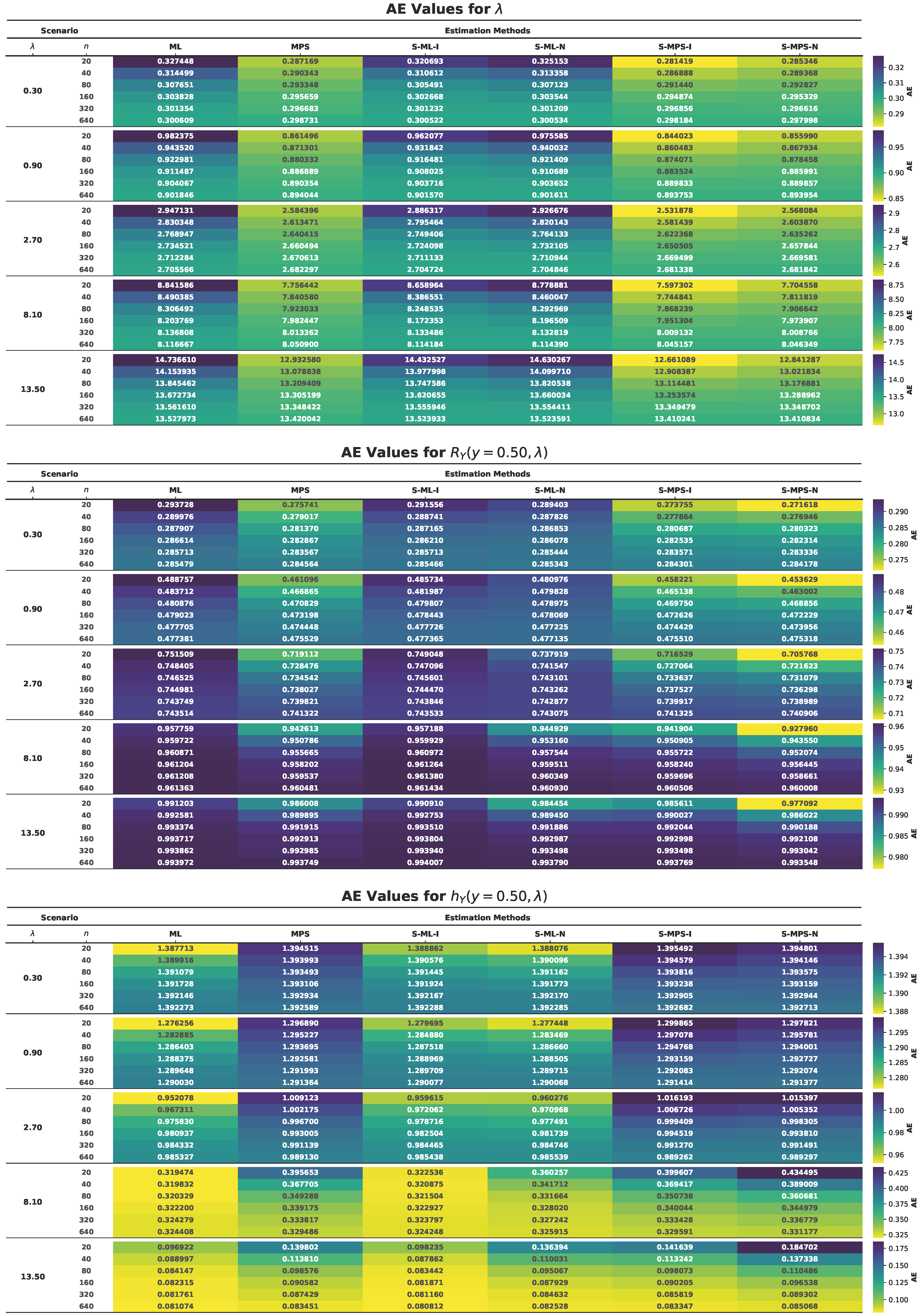
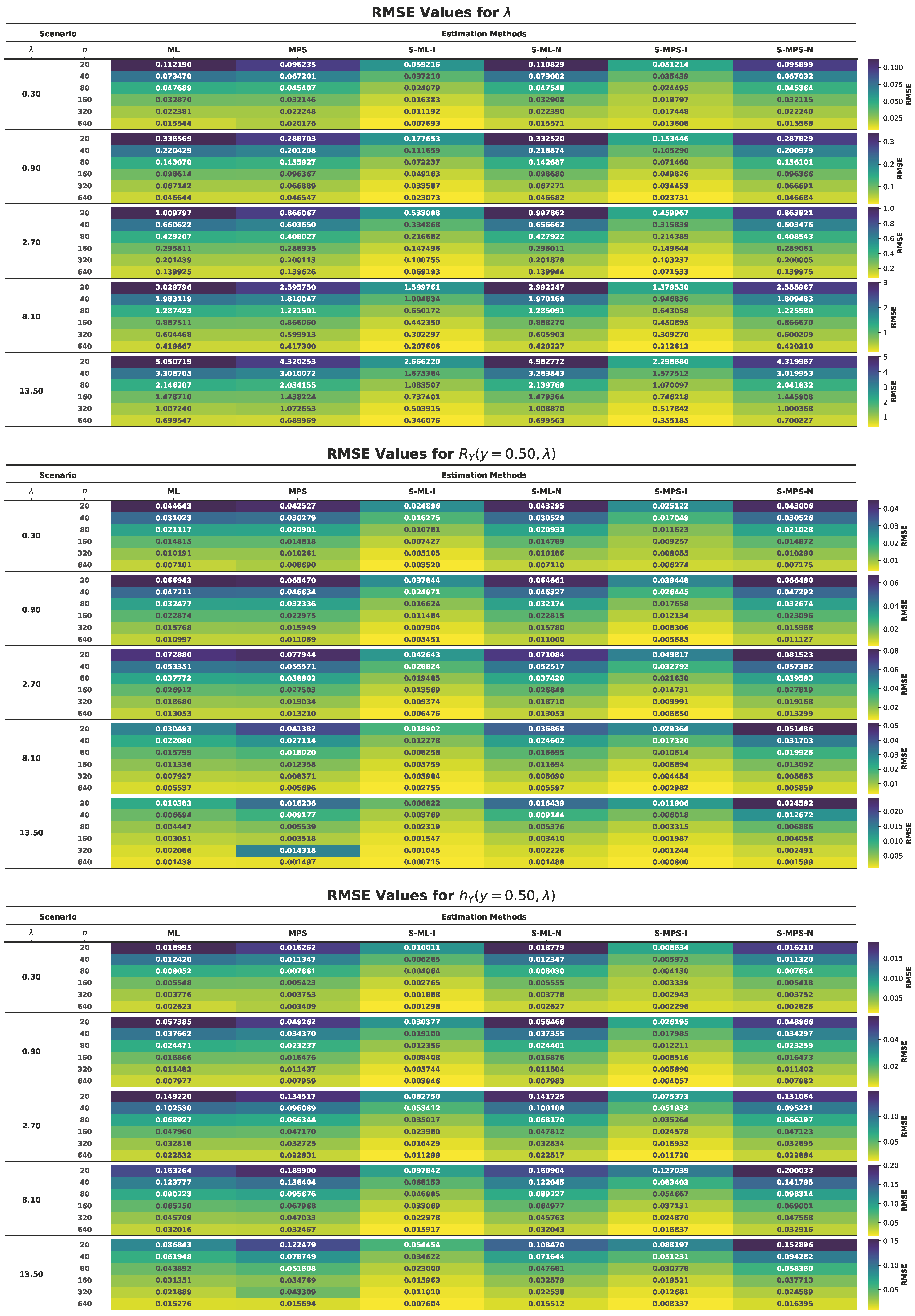
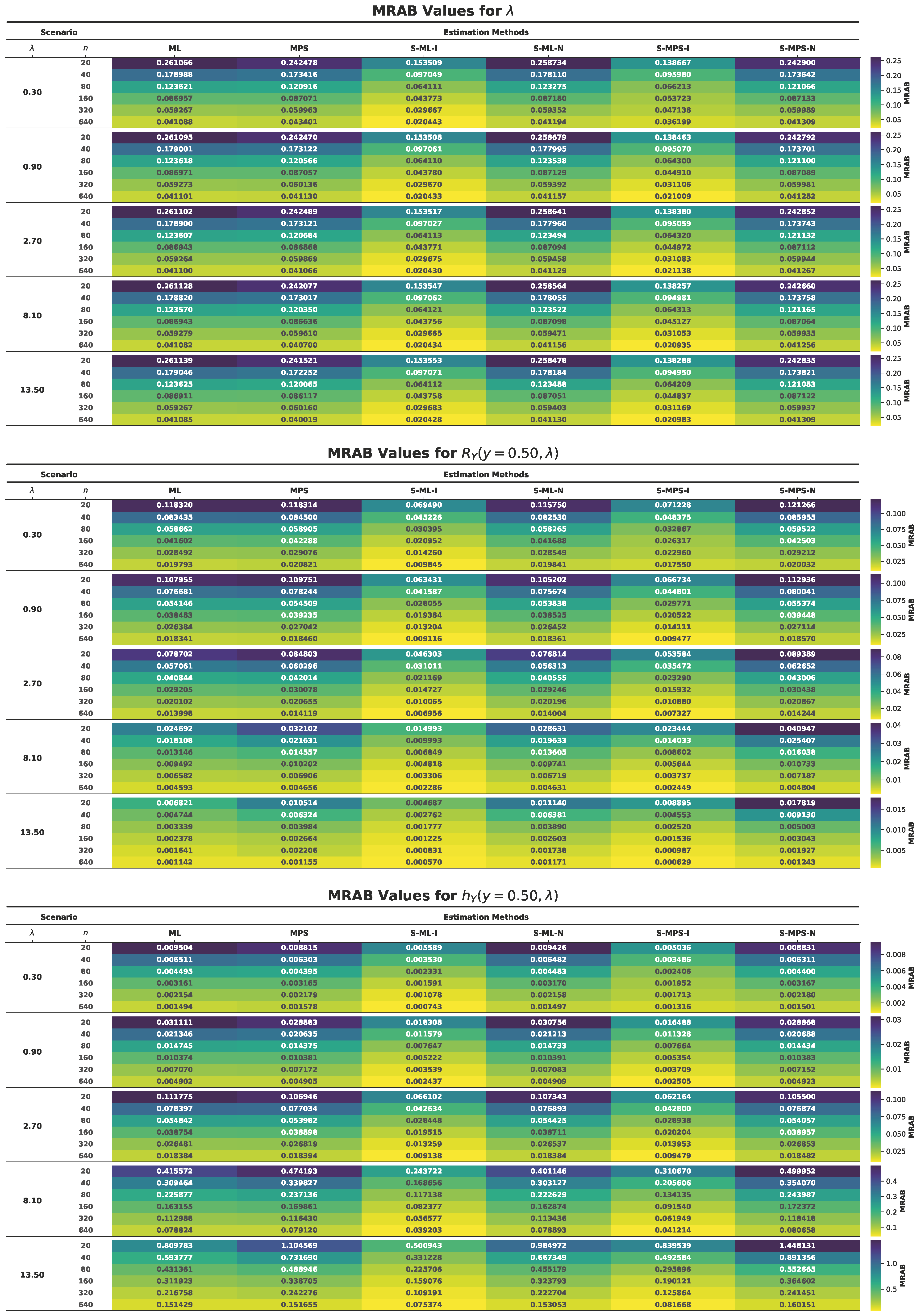
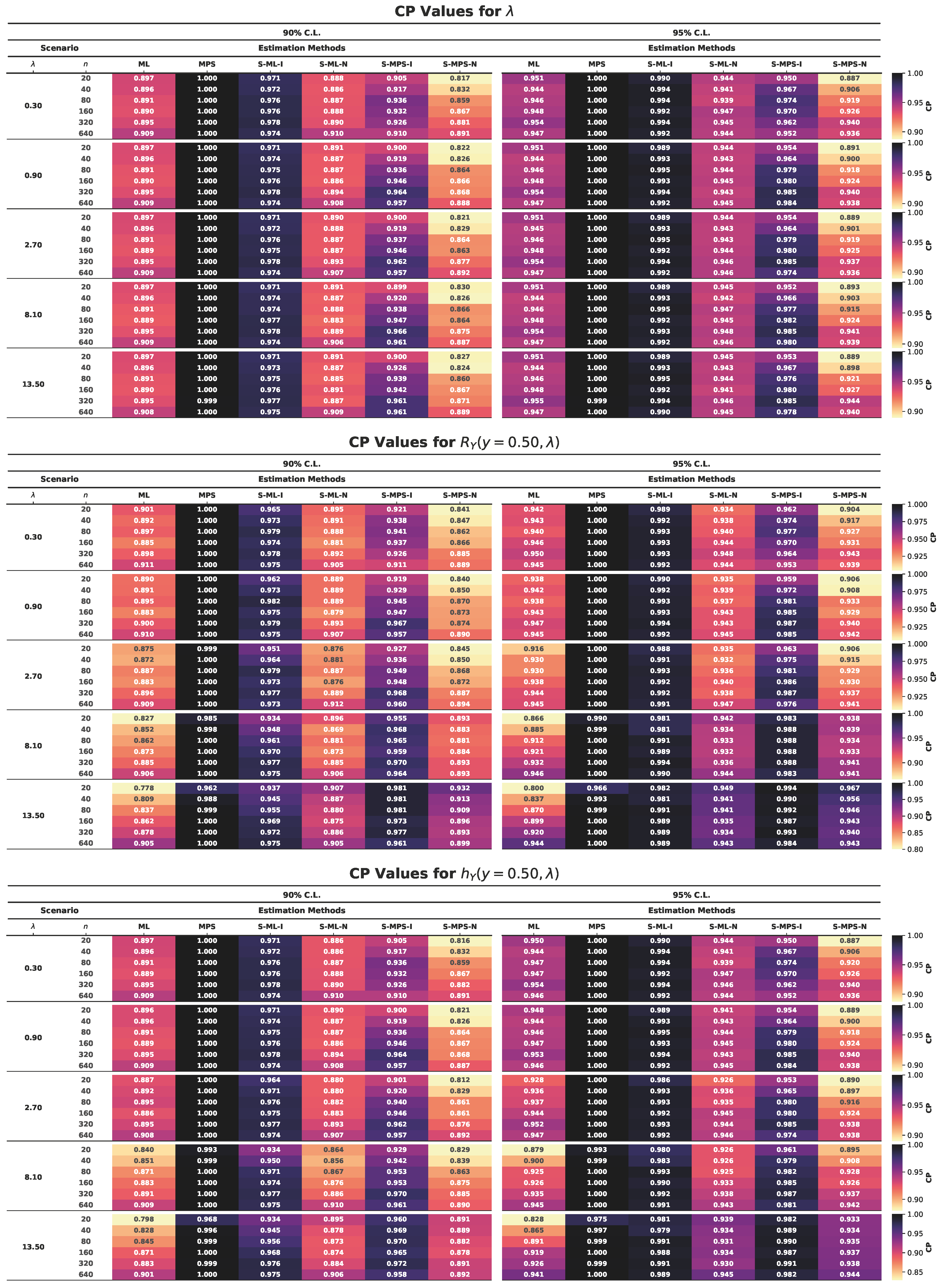
The summary of the simulation results, in the form of heatmap visualizations in Figure 7, Figure 8, Figure 9, Figure 10 and Figure 11, gives an overall comparison of the performance of the estimators with all the configurations. The analysis is done in terms of the already defined metrics, which allow for performing a joint assessment of the point estimation accuracy and interval reliability. The main conclusions can be summarized as follows:

• All estimators converge to the true parameter values with an increase in sample size, which confirms their consistency in estimating both the parameter, $\lambda$ and the functions, $R_Y(y,\lambda )$ and $h_Y(y,\lambda )$.
• Bayesian estimators using informative priors (S-ML-I and S-MPS-I) are also more accurate, and therefore their estimates are closer to the true values than the classical and non-informative Bayesian estimators.
• The values of RMSE are monotonically decreasing with the increase in sample size, showing an increase in precision. Bayesian estimators have the lowest RMSE in all configurations, the next is ML, and lastly the variability of the MPS-based estimators is rather high.
• The values of MRAB decrease in a systematic manner with an increase in the sample size and tend to be zero for all estimators. Informative Bayesian estimators display the quickest reduction of bias, especially when using small sample sizes.
• The values of AL decrease as the sample size is increased. Bayesian HPD CRIs that make use of informative priors are always shorter, meaning that they provide more efficient quantification of uncertainty than classical and MPS-based intervals.
• The values of CP tend to reach the nominal levels of $90\%$ and $95\%$ as the sample size increases. Informative Bayesian estimators have the best coverage, and ML under-covers and MPS over-covers in small data sets.
• Informative Gamma priors significantly increase the accuracy of estimations, minimize bias, and perform better on the interval compared to the use of Jeffreys’ priors, which are less stable in small samples.
• In all the performance criteria, the estimators may be ranked as follows:

  $$\mathrm{S}\text{-}\mathrm{ML}\text{-}\mathrm{I}\gtrsim \mathrm{S}\text{-}\mathrm{MPS}\text{-}\mathrm{I}>\mathrm{ML}>\mathrm{S}\text{-}\mathrm{ML}\text{-}\mathrm{N}>\mathrm{MPS}\gtrsim \mathrm{S}\text{-}\mathrm{MPS}\text{-}\mathrm{N}.$$
• The patterns observed do not change when using the parameter of the model $\lambda$ or the model functions $R_Y(y,\lambda )$ and $h_Y(y,\lambda )$ and the patterns are also consistent, which means that there is a consistent inferential performance in the various aspects of the model.
• Bayesian estimation under informative priors, especially the S-ML-I, offers the most efficient and accurate estimation of the UASED model, especially when the sample size is small.

Figure 7. Heatmaps of AE values for $\lambda$ (top), $R_Y(y,\lambda )$ (center), and $h_Y(y,\lambda )$ (bottom).

Figure 7. Heatmaps of AE values for $\lambda$ (top), $R_Y(y,\lambda )$ (center), and $h_Y(y,\lambda )$ (bottom).

Figure 8. Heatmaps of RMSE values for $\lambda$ (top), $R_Y(y,\lambda )$ (center), and $h_Y(y,\lambda )$ (bottom).

Figure 8. Heatmaps of RMSE values for $\lambda$ (top), $R_Y(y,\lambda )$ (center), and $h_Y(y,\lambda )$ (bottom).

Figure 9. Heatmaps of MRAB values for $\lambda$ (top), $R_Y(y,\lambda )$ (center), and $h_Y(y,\lambda )$ (bottom).

Figure 9. Heatmaps of MRAB values for $\lambda$ (top), $R_Y(y,\lambda )$ (center), and $h_Y(y,\lambda )$ (bottom).

Figure 10. Heatmaps of AL values for $\lambda$ (top), $R_Y(y,\lambda )$ (center), and $h_Y(y,\lambda )$ (bottom).

Figure 10. Heatmaps of AL values for $\lambda$ (top), $R_Y(y,\lambda )$ (center), and $h_Y(y,\lambda )$ (bottom).

Figure 11. Heatmaps of CP values for $\lambda$ (top), $R_Y(y,\lambda )$ (center), and $h_Y(y,\lambda )$ (bottom).

Figure 11. Heatmaps of CP values for $\lambda$ (top), $R_Y(y,\lambda )$ (center), and $h_Y(y,\lambda )$ (bottom).

7. Real-World Application

In this section, we analyze a real-world reliability dataset to evaluate the inferential performance and modeling flexibility of the proposed UASED. The data comprise the failure times of 50 devices subjected to a life test starting at $y=0$, originally reported in [28,29]. The observed lifetimes are summarized below:

0.1, 0.2, 1, 1, 1, 1, 1, 2, 3, 6, 7, 11, 12, 18, 18, 18, 18, 18, 21, 32, 36, 40, 45, 46, 47, 50, 55, 60, 63, 63, 67, 67, 67, 67, 72, 75, 79, 82, 82, 83, 84, 84, 84, 85, 85, 85, 85, 85, 86, 86.

Since the theoretical basis of the UASED is limited to the open unit interval $(0,1)$, the raw data needed to be transformed before estimation of the model. A min–max normalization was used to fit the data to the range of $[0,1]$:

$$y_i^{*}={\displaystyle \frac{y_i-min\left(\mathbf{y}\right)}{max\left(\mathbf{y}\right)-min\left(\mathbf{y}\right)}},i=1,\dots ,n.$$

Any boundary values (0 or 1) that were the result of the transformation were eliminated so as to be consistent with the support of the distribution. This linear rescaling maintains the inherent stochastic structure and relative rank of the observations and makes it easy to make valid inferences. The analysis data is normalized and shown in the following:

0.00116, 0.01048, 0.01048, 0.01048, 0.01048, 0.01048, 0.02212, 0.03376, 0.06868, 0.08033, 0.12689, 0.13853, 0.20838, 0.20838, 0.20838, 0.20838, 0.20838, 0.24331, 0.37136, 0.41793, 0.46449, 0.52270, 0.53434, 0.54598, 0.58091, 0.63912, 0.69732, 0.73225, 0.73225, 0.77881, 0.77881, 0.77881, 0.77881, 0.83702, 0.87194, 0.91851, 0.95343, 0.95343, 0.96508, 0.97672, 0.97672, 0.97672, 0.98836, 0.98836, 0.98836, 0.98836, 0.98836.

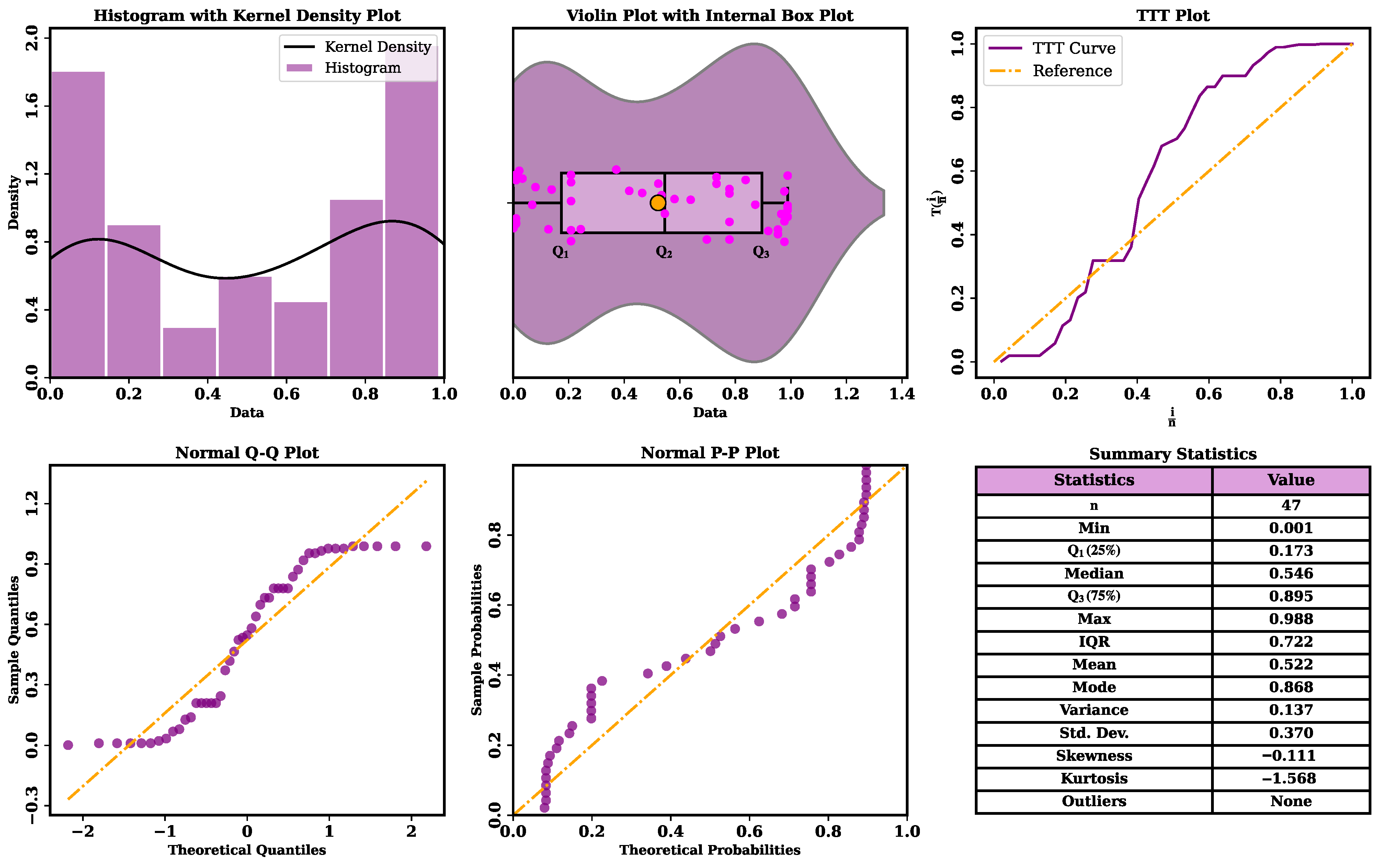
To preliminarily investigate the transformed failure-time data, nonparametric graphical tools were utilized before performing the parametric modeling, as presented in Figure 12. The Histogram with Kernel Density shows that it is clearly bimodal, with the probability mass being concentrated at the boundaries of $(0,1)$. The pattern is supported by the fact that, according to the Violin Plot, there are clustered failures, but these are not evenly distributed. These findings are supported by the Summary Statistics table below in Figure 12, as the negative kurtosis values depict a platykurtic form with light tails, skewness is for near-symmetry, and the Box Plot plus the variance depict high dispersion in the normalized lifetimes. The Total Time on Test (TTT) Plot does not follow the diagonal, meaning that the hazard rate has a bathtub-shaped profile with the following characteristics: (i) excessively high early failure intensity, (ii) a steady middle phase and (iii) an increasing wear-out phase. Lastly, the systematic deviations of the 45-degree line are observed in the Normal Q–Q and P–P Plots, especially in tails. Together with the bimodality that was observed, these findings prove that the usual symmetric or unimodal models are insufficient, and thus the adaptable UASED is used.

The estimation of the unknown parameter of the UASED is now done using the ML method. To evaluate them comparatively, four alternative unit distributions were fitted to the same normalized data set: the Unit-Weibull Distribution (UWD) [30], the Unit Inverse Weibull Distribution (UIWD) [31], the Transmuted Unit Distribution (TUD) [32], and the Unit Power Distribution (UPD) [33]. The ML estimates, along with standard errors (SEs) of the model estimates, values of $-2$ times the maximization process of the log-likelihood ($-2\ell$), and a combination of penalized likelihood-based model selection criteria, were obtained using the same numerical optimization processes and convergence criteria to ensure methodological consistency and fairness in model comparison. The Akaike Information Criterion (AIC), the Consistent AIC (CAIC), the Bayesian Information Criterion (BIC) and the Hannan–Quinn Information Criterion (HQIC) were used in evaluating the model adequacy. To further test the hypothesis, the values of empirical distribution functions are also provided in

Table 3. ML estimates with different goodness-of-fit results for failure-time data.

Model	UASED {$\mathit{\lambda }$}	UWD {$\mathit{\lambda },\mathit{\theta }$}	UIWD {$\mathit{\lambda },\mathit{\theta }$}	TUD {$\mathit{\lambda }$}	UPD {$\mathit{\lambda }$}
Est.	$1.0235$	$0.9989,0.6408$	$0.3746,0.5067$	$-0.0800$	$0.7414$
S.E.	$0.1932$	$0.1535,0.0756$	$0.0809,0.0550$	$0.1961$	$0.1081$
$-\mathbf{2}\ell$	$-22.8896$	$-21.9090$	$-6.8715$	$-0.1657$	$-4.6601$
AIC	$-20.8896$	$-17.9090$	$-2.8715$	$1.8343$	$-2.6601$
CAIC	$-20.8007$	$-17.6363$	$-2.5988$	$1.9232$	$-2.5713$
BIC	$-19.0394$	$-14.2087$	$0.8288$	$3.6844$	$-0.8100$
HQIC	$-20.1934$	$-16.5166$	$-1.4791$	$2.5305$	$-1.9639$
${\mathit{A}}^{\mathit{*}}$	$0.6124$	$0.6697$	$1.9677$	$5.7062$	$6.2151$
${\mathit{W}}^{\mathit{*}}$	$0.0752$	$0.0781$	$0.3151$	$0.4852$	$0.6671$
$\mathit{K}$–$\mathit{S}$	$0.0940$	$0.1016$	$0.1716$	$0.1839$	$0.2192$
p-value	$0.7659$	$0.6795$	$0.1112$	$0.0729$	$0.0183$

, i.e., the Anderson–Darling ($A^{*}$), Cramér–von Mises ($W^{*}$), and Kolmogorov–Smirnov (K–S) statistics are also given, with the corresponding K–S test p-values.

The numerical results reported in Table 3 indicate that the UASED attains the smallest values for all considered information criteria (AIC, CAIC, BIC, and HQIC). This suggests that the UASED offers the most efficient balance between model complexity and goodness of fit under penalized likelihood frameworks. Furthermore, the UASED yields the highest K–S p-value ($0.7659$), indicating no statistically significant deviation between the empirical and theoretical distributions at conventional significance levels.

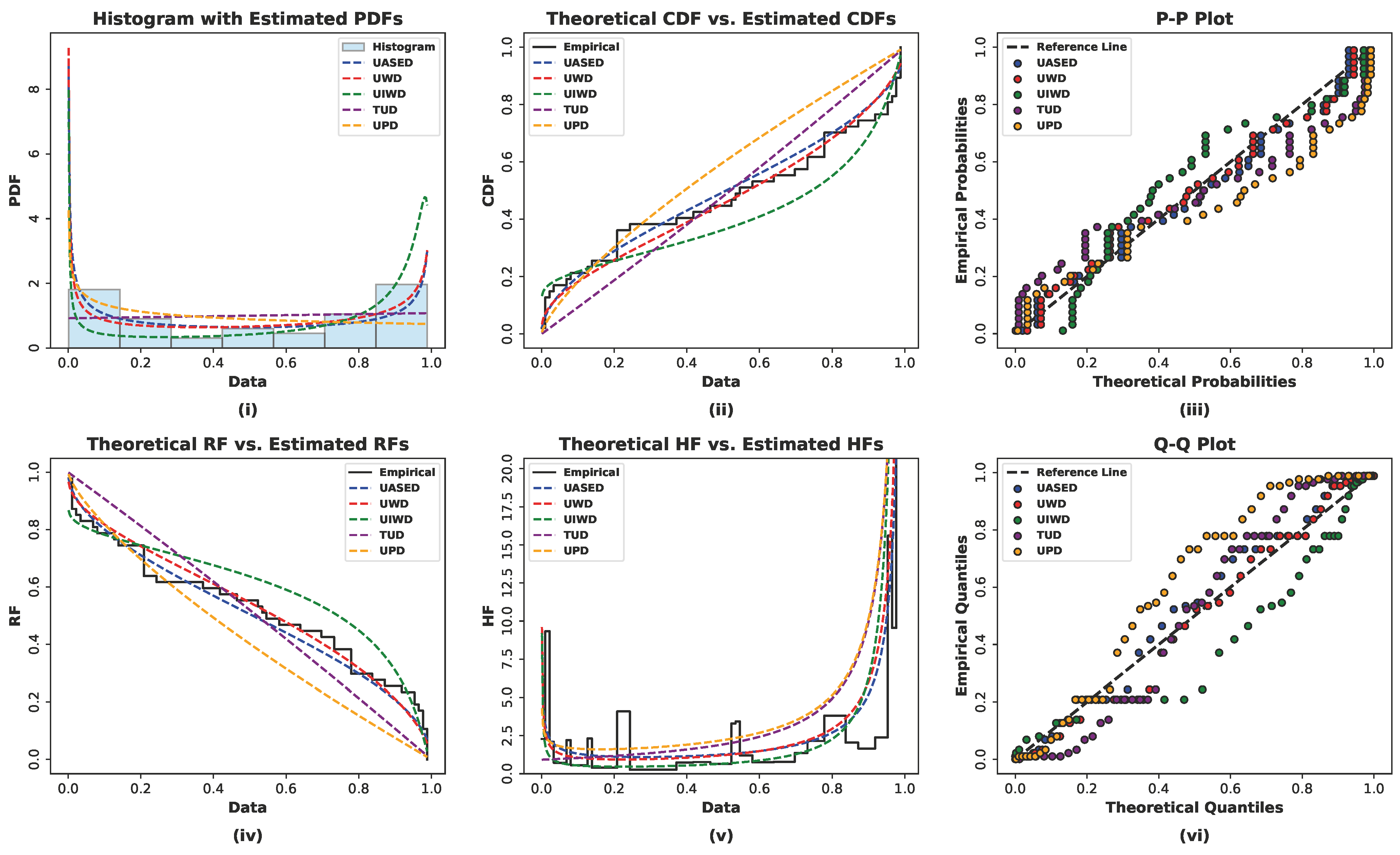
The fitted models are compared graphically in Figure 13. According to the Histogram with Estimated PDFs (i), the UASED approaches the empirical distribution much more closely, especially at the point of the unit interval, and the competing models have observable point-wise discrepancies in capturing the general appearance of data. According to the analysis of the Theoretical CDF vs. Estimated CDFs (ii), it becomes clear that the UASED offers the closest match to the empirical CDF at all support levels, whereas other models show apparent differences. The P–P Plot (iii) and Q–Q Plot (vi) demonstrate that the UASED has the nearest agreement with empirical distribution across the full support, and especially in the tails.

This implies that the proposed model is more fitted to the data than other competing distributions. Similarly, the Theoretical RF vs. Estimated RFs (iv) indicates that the UASED has the ability to reproduce the empirical survival behavior, whereas the rest of the models have deviations, especially in the later stages of the life test. On the hazard dynamics, as is shown in the figure, the Theoretical HF vs. Estimated HFs (v) indicates that the UASED is well-suited to accommodate the non-monotonic, bathtub-shaped hazard structure, as observed previously in the TTT plot. The high initial failure rate and the enhancement of risk at an older age are recapitulated in the estimated hazard function. Conversely, some of the competing models either flatten the concentration of failure at the start or poorly characterize the wear-out. Altogether, in the studied failure-time data, the presence of a non-monotonic and bathtub-shaped hazard structure is highly pronounced. The overall findings of the nonparametric exploration, the ML estimation, the penalized likelihood criteria, the goodness-of-fit measures, and the graphical diagnostics all point to the fact that the UASED offers the most sufficient representation among the models in question. The UASED has a high level of information criteria and the best competitive statistics, with the highest K–S p-value; and the UASED exhibits a high level of graphical conformity to the empirical distribution; therefore, it emerges as a viable and parsimonious model to use when modeling lifetime data with complex hazard dynamics.

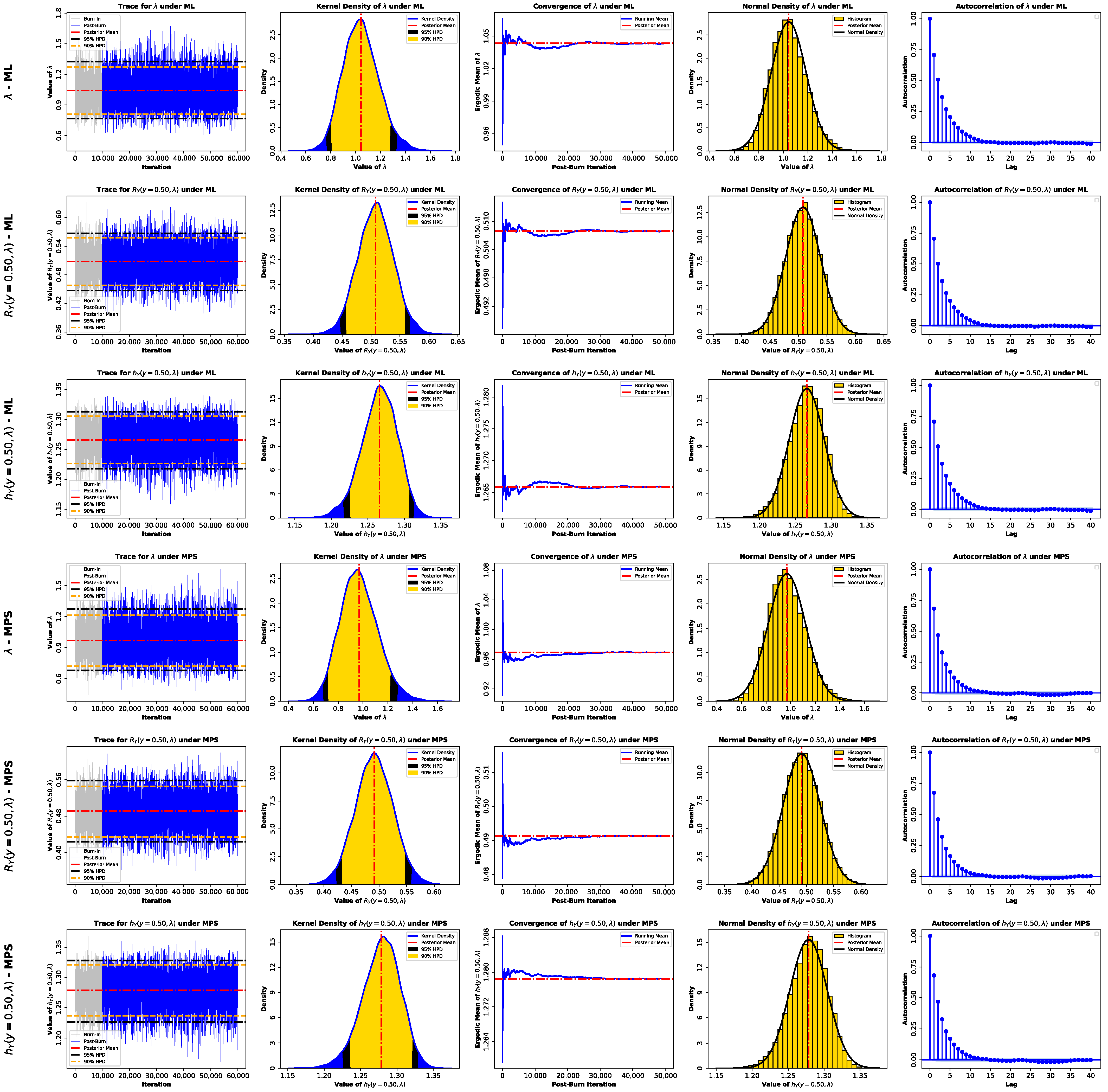
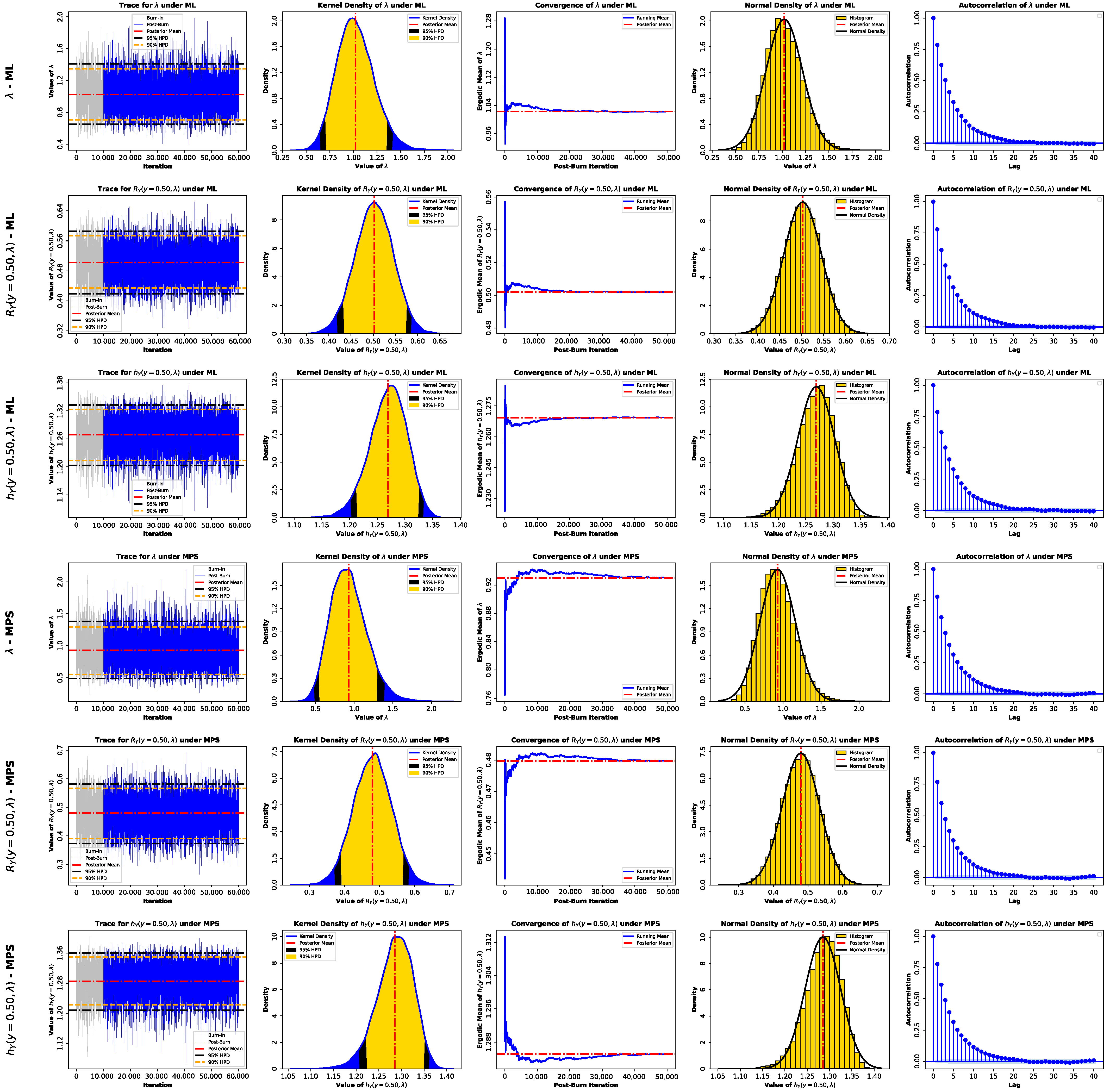
To further test the inferential performance of the proposed model, the parameter $\lambda$, as well as $R_Y(y,\lambda )$ and $h_Y(y,\lambda )$ at $y=0.50$, are all subjected to a Bayesian analysis. An informative Gamma prior and a non-informative Jeffreys’ prior are both used to evaluate how sensitive the inference is to specifying prior. Estimation is done by posterior estimation through the MCMC method of the ML and MPS frameworks.

Table 4. Classical and Bayesian inference of $\lambda$, $R_Y(y,\lambda )$, and $h_Y(y,\lambda )$ at $y=0.50$ for the failure times data.

Par.	Methods	Est.	S.E.	90% C.L.			95% C.L.
				Low.	Upp.	Wid.	Low.	Upp.	Wid.
$\lambda$	ML	1.0235	0.1932	0.7057	1.3413	0.6356	0.6449	1.4022	0.7574
	MPS	0.9327	0.2333	0.5489	1.3164	0.7676	0.4753	1.3900	0.9146
	S-ML-I	1.0432	0.1432	0.8107	1.2736	0.4629	0.7675	1.3249	0.5574
	S-ML-N	1.0227	0.1969	0.7072	1.3471	0.6399	0.6503	1.4090	0.7588
	S-MPS-I	0.9693	0.1523	0.7213	1.2147	0.4934	0.6795	1.2742	0.5947
	S-MPS-N	0.9303	0.2331	0.5514	1.2938	0.7424	0.4877	1.3814	0.8937
$R_Y(y,\lambda )$	ML	0.5052	0.0419	0.4362	0.5741	0.1380	0.4229	0.5874	0.1644
	MPS	0.4848	0.0540	0.3960	0.5736	0.1776	0.3789	0.5906	0.2117
	S-ML-I	0.5079	0.0306	0.4577	0.5576	0.0999	0.4470	0.5670	0.1201
	S-ML-N	0.5021	0.0427	0.4341	0.5739	0.1398	0.4187	0.5855	0.1668
	S-MPS-I	0.4913	0.0342	0.4339	0.5458	0.1119	0.4236	0.5580	0.1344
	S-MPS-N	0.4797	0.0537	0.3908	0.5666	0.1758	0.3729	0.5823	0.2093
$h_Y(y,\lambda )$	ML	1.2692	0.0331	1.2148	1.3236	0.1088	1.2044	1.3340	0.1296
	MPS	1.2848	0.0399	1.2191	1.3504	0.1313	1.2065	1.3630	0.1565
	S-ML-I	1.2658	0.0245	1.2264	1.3056	0.0792	1.2176	1.3130	0.0954
	S-ML-N	1.2693	0.0337	1.2138	1.3233	0.1095	1.2032	1.3330	0.1298
	S-MPS-I	1.2785	0.0261	1.2365	1.3209	0.0844	1.2263	1.3280	0.1017
	S-MPS-N	1.2851	0.0399	1.2229	1.3498	0.1269	1.2079	1.3606	0.1527

summaries reported in the rear indicate that all the estimation methods are in strong agreement and prove that the proposed model is stable. Specifically, the standard errors and credible intervals of the Bayesian estimators under the SEL function are smaller, which speaks in favor of the higher precision of the estimations. The informative prior, as anticipated, generates more concentrated posterior distributions than the Jeffreys’ prior, but there is a negligible difference in the inferences made overall. The MCMC diagnostics in Figure 14 and Figure 15 demonstrate good convergence and effectiveness in sampling under both priors. The trace plots are stable and stationary in nature, the posterior densities are unimodal and the running means approach constant values quickly. Autocorrelation functions approach the value of zero, meaning that there is weak serial dependence. In comparison to the informative prior of the case in Figure 14, the noninformative prior of the case in Figure 15 has slightly more dispersed posterior distributions and slower autocorrelation decay, which can be attributed to increased uncertainty. Nevertheless, the findings are similar between the ML and MPS frameworks. The Bayesian analysis, in general, endorses the strength and efficiency of the proposed UASED, with the informative prior rendering precision and the non-informative prior giving reliable and consistent inferences.

8. Conclusions

The UASED presented in this paper is a simple but flexible unit-interval data model, obtained by a monotone transformation and with explicit distributional characterizations. The main elements of mathematics, such as reliability functions and measurement of information, have been developed to explain the behavior of the model and its practical interpretation. In order to facilitate principled inference, the study formulated and analyzed both traditional estimation methods (likelihood- and spacing-based), as well as a Bayesian model that was employed using Metropolis–Hastings sampling, and its performance was evaluated by simulation and empirical examples. Collectively, the findings indicate that the proposed distribution offers an analytically convenient and conceptually consistent supplement to the arsenal of tools to model the results of finite lifetime and proportion-type outcomes, whereas the complementing inferential processes support trustworthy estimation and quantification of uncertainty. In general, the paper secures the principles underpinning unit-bounded distributional modeling by providing a highly motivated, practically implementable substitute that facilitates sound applied investigation. Although the suggested UASED has the advantage of analytical tractability and flexibility in modeling unit-interval data, it has only a single-parameter form that might not be as flexible as multi-parameter forms. It can be possible in future studies to use multiparameter extensions, regression-type formulations that include covariates, or even inflated and mixture versions to handle boundary observations.

References

1. Bayes, T. An essay towards solving a problem in the doctrine of chances. Philos. Trans. R. Soc. 1763, 53, 370–418. [Google Scholar] [CrossRef]
2. Kumaraswamy, P. A generalized probability density function for double-bounded random processes. J. Hydrol. 1980, 46, 79–88. [Google Scholar] [CrossRef]
3. Topp, C.W.; Leone, F.C. A family of J-shaped frequency functions. J. Am. Stat. Assoc. 1955, 50, 209–219. [Google Scholar] [CrossRef]
4. Johnson, N.L.; Kotz, S.; Balakrishnan, N. Continuous Univariate Distributions, 2nd ed.; Wiley: Hoboken, NJ, USA, 1995; Volume 2. [Google Scholar]
5. Ghitany, M.E.; Mazucheli, J.; Menezes, A.F.B.; Alqallaf, F. The Unit-Inverse Gaussian distribution: A new alternative to two-parameter distributions on the unit interval. Commun. Stat. Theory Methods 2019, 48, 3423–3438. [Google Scholar] [CrossRef]
6. Mazucheli, J.; Menezes, A.F.B.; Chakraborty, S. On the one-parameter Unit-Lindley distribution and its associated regression model for proportion data. J. Appl. Stat. 2019, 46, 700–714. [Google Scholar] [CrossRef]
7. Mazucheli, J.; Menezes, A.F.B.; Fernandes, L.B.; de Oliveira, R.P.; Ghitany, M.E. The Unit-Weibull distribution as an alternative to the Kumaraswamy distribution for the modeling of quantiles conditional on covariates. J. Appl. Stat. 2019, 47, 954–974. [Google Scholar] [CrossRef]
8. Mazucheli, J.; Menezes, A.F.; Dey, S. Unit-Gompertz distribution with applications. Statistica 2019, 79, 25–43. [Google Scholar]
9. Consul, P.C.; Jain, G.C. On the log-gamma distribution and its properties. Stat. Hefte 1971, 12, 100–106. [Google Scholar] [CrossRef]
10. Rahman, M.M. Arcsine-G family of distributions. J. Stat. Appl. Prob. Lett 2021, 8, 169–179. [Google Scholar]
11. Rényi, A. On Measures of Entropy and Information. In Proceedings of the Fourth Berkeley Symposium on Mathematical Statistics and Probability, Volume 1: Contributions to the Theory of Statistics; University of California Press: Berkeley, CA, USA, 1961; pp. 547–561. [Google Scholar]
12. Arimoto, S. Information-theoretical considerations on estimation problems. Inf. Control 1971, 19, 181–194. [Google Scholar] [CrossRef]
13. Tsallis, C. Possible generalization of Boltzmann–Gibbs statistics. J. Stat. Phys. 1988, 52, 479–487. [Google Scholar] [CrossRef]
14. Ibrahim, R. Water Engineering Modeling Controlled by Generalized Tsallis Entropy. Montes Taurus J. Pure Appl. Math. 2021, 3, 227–237. [Google Scholar]
15. Havrda, J.; Charvát, F.S. Quantification method of classification processes: Concept of structural-entropy. Kybernetika 1967, 3, 30–35. [Google Scholar]
16. Mathai, A.M.; Haubold, H.G. On generalized distributions and pathways. Phys. Lett. 2008, 372, 2109–2113. [Google Scholar] [CrossRef]
17. Shannon, C.E. A Mathematical Theory of Communication. Bell Syst. Tech. J. 1948, 27, 379–423. [Google Scholar] [CrossRef]
18. Gradshteyn, I.S.; Ryzhik, I.M. Table of Integrals, Series, and Products, 8th ed.; Academic Press: New York, NY, USA, 2014. [Google Scholar]
19. Cheng, R.C.H.; Amin, N.A.K. Estimating parameters in continuous univariate distribution with a shifted origin. J. R. Stat. Soc. 1983, 45, 394–403. [Google Scholar] [CrossRef]
20. Virtanen, P.; Gommers, R.; Oliphant, T.E.; Haberland, M.; Reddy, T.; Cournapeau, D.; Burovski, E.; Peterson, P.; Weckesser, W.; Bright, J.; et al. SciPy 1.0: Fundamental algorithms for scientific computing in Python. Nat. Methods 2020, 17, 261–272. [Google Scholar] [CrossRef] [PubMed]
21. Held, L.; Sabanés Bové, D. Applied Statistical Inference: Likelihood and Bayes; Springer: Berlin/Heidelberg, Germany, 2014. [Google Scholar]
22. Ranneby, B. The maximum spacing method. An estimation method related to the maximum likelihood method. Scand. J. Stat. 2016, 11, 93–112. [Google Scholar]
23. Webel, K.; Greene, W.H. Econometric analysis. Stat. Pap. 2011, 52, 983–984. [Google Scholar] [CrossRef]
24. Dey, S.; Dey, T.; Luckett, D.J. Statistical inference for the generalized inverted exponential distribution based on upper record values. Math. Comput. Simul. 2016, 120, 64–78. [Google Scholar] [CrossRef]
25. Lynch, S.M. Introduction to Applied Bayesian Statistics and Estimation for Social Scientists, 1st ed.; Statistics for Social and Behavioral Sciences; Springer: New York, NY, USA, 2007. [Google Scholar]
26. Tierney, L. Markov chains for exploring posterior distributions. Ann. Stat. 1994, 22, 1701–1728. [Google Scholar] [CrossRef]
27. Gilks, W.R.; Richardson, S.; Spiegelhalter, D. Markov Chain Monte Carlo in Practice; Chapman and Hall/CRC: Boca Raton, FL, USA, 1995. [Google Scholar]
28. Aarset, M.V. How to Identify a Bathtub Hazard Rate. IEEE Trans. Reliab. 1987, 36, 106–108. [Google Scholar] [CrossRef]
29. González-Hernández, I.J.; Méndez-González, L.C.; Granillo-Macías, R.; Rodríguez-Muñoz, J.L.; Pacheco-Cedeño, J.S. A New Generalization of the Uniform Distribution: Properties and Applications to Lifetime Data. Mathematics 2024, 12, 2328. [Google Scholar] [CrossRef]
30. Mazucheli, J.; Menezes, A.F.B.; Ghitany, M.E. The Unit-Weibull distribution and associated inference. J. Appl. Probab. Stat. 2018, 13, 1–22. [Google Scholar]
31. Ribeiro-Reis, L.D. The Unit Inverse Weibull Distribution and its Associated Regression Model. J. Econom. Stat. 2023, 3, 55–68. [Google Scholar]
32. Shaw, W.T.; Buckley, I.R.C. The alchemy of probability distributions: Beyond Gram–Charlier expansions, and a skew-kurtotic-normal distribution from a rank transmutation map. arXiv 2009, arXiv:0901.0434. [Google Scholar]
33. Ahsanullah, M. Handbook on Univariate Statistical Distributions; Ewings Publishing LLC: Metairie, LA, USA, 2022. [Google Scholar]
Figure 1. PDF (left) and CDF (right) at different values of the parameter λ .
Axioms 15 00218 g001
Figure 2. RF (left) and HF (right) of the UASED for various values of λ .
Axioms 15 00218 g002
Figure 5. Profile of the log-likelihood and log product of spacings with their corresponding first derivatives. The black points denote the ML and MPS estimators for λ true = 2.70 .
Axioms 15 00218 g005
Figure 6. Plots of prior, likelihood (or product of spacings), and posterior distributions at λ = 2.70 .
Axioms 15 00218 g006
Figure 12. Non-parametric diagnostic plots and descriptive statistics for the normalized failure-time data.
Axioms 15 00218 g012
Figure 13. Graphical diagnostic graphs for determining the goodness-of-fit and the overall adequacy of the fitted distributional models to the normalized failure-time data.
Axioms 15 00218 g013
Figure 14. MCMC diagnostic plots for the posterior parameter estimation of λ , R Y ( y , λ ) , and h Y ( y , λ ) under ML and MPS methods using an informative Gamma prior.
Axioms 15 00218 g014
Figure 15. MCMC diagnostic plots for the posterior parameter estimation of λ , R Y ( y , λ ) , and h Y ( y , λ ) under ML and MPS methods using a noninformative Jeffery’s prior.
Axioms 15 00218 g015