The Dynamics of a Switched IPM Model with Predation-Induced Fear and Seasonal Birth in a Pest Population

Abstract

IPM (Integrated Pest Management) strategies present a good theoretical framework for sustainably controlling pest populations. In this paper, we propose a switched IPM model with predation-induced fear and seasonally birth in a pest population. Employing theories of impulsive differential equations, we gain evidence showing that the pest-eradication solution $(0,\overline{y\left(t\right)})$ of the investigated system is GAS. The investigated system is also proven to be persistent. Our results provide new methods for IPM strategies.

1. Introduction

Biological control in agricultural management has been implemented for at least one hundred and twenty years across the whole world, which has introduced beneficial biological control agents to control pests and weeds [1,2,3,4,5]. Biological control can effectively suppress pest populations in agricultural production. Based on these findings, Liu and Chen [6] proposed a prey–predator model with impulsive effects for biological control.

However, biological control strategies prove less effective during pest outbreaks; therefore, integrated pest management strategies are introduced to control pest populations. In all, pesticides are useful for their ability to kill most pests, and sometimes, they may provide the only valid method for preventing economic losses. The essence of integrated pest management is to take prevention as the core, combine physical, chemical, biological, and cultural means, and achieve a balance between pest population control and environmental protection through scientific monitoring and dynamic adjustments [7,8,9]. Infected pest populations and spraying pesticides have also been introduced into IPM strategies; Jiao et al. [10] have put forward a new pest management SI model that involves releasing an infected pest population and spraying pesticides at different moments. Tang et al. [11] investigated integrated pest management models, with pesticides having residual effects. Further, Jiao et al. [12] presented an impulsive IPM model with many instances of releasing a natural enemy and spraying pesticides.

Influenced by the seasonal changes every year, there are very obvious phenomena of migration, birth pulse, hibernation, and so on of populations, which are often regular activities for animals to adapt to climate changes and food shortages and to ensure their successful reproduction [13,14,15,16]. Therefore, Jiao et al. [17] established a seasonal switched predator–prey model with impulsive migration. Generally, there are two ways in which predation influences prey, which are directly killing the prey and predation-induced fear. Many experiments have shown that the predation-induced fear has a larger impact on prey than directly killing them [18,19], and predation-induced fear was also introduced into predator–prey systems [20,21,22].

All in all, although there has been much research on the mathematical models of integrated pest management, few authors have introduced seasonal switching and predation-induced fear into IPM dynamical models. Furthermore, predator–prey models with fear effects also fail to account for seasonal changes and the nonlinear impulsive release of a predator population. In this paper, we consider a switched IPM model with predation-induced fear, seasonal birth in a pest population, and the nonlinear releasing of a natural enemy.

2. The Model

In this section, we introduce a switched IPM model with predation-induced fear and seasonal birth in a pest population, as follow:

$$\left\{\begin{array}{c}\left.\begin{array}{c}{\displaystyle \frac{dx\left(t\right)}{dt}=-d_{1}x\left(t\right)-\frac{{\beta }_{1}x\left(t\right)y\left(t\right)}{1+{\gamma }_{1}x\left(t\right)},}\hfill \\ {\displaystyle \frac{dy\left(t\right)}{dt}=-d_{2}y\left(t\right)+\frac{k_1{\beta }_{1}x\left(t\right)y\left(t\right)}{1+{\gamma }_{1}x\left(t\right)},}\hfill \end{array}\right\}t\in (n\upsilon ,(n+l_1)\tau ],\hfill \\ \left.\begin{array}{c}{\displaystyle ▵x\left(t\right)=bx\left(t\right),}\hfill \\ {\displaystyle ▵y\left(t\right)=0,}\hfill \end{array}\right\}t=(n+l_1)\tau ,\hfill \\ \left.\begin{array}{c}{\displaystyle \frac{dx\left(t\right)}{dt}=x\left(t\right)(\frac{a_1}{1+{\delta }_{1}y\left(t\right)}-b_{1}x\left(t\right))-\frac{{\beta }_{2}x\left(t\right)y\left(t\right)}{1+{\gamma }_{2}x\left(t\right)},}\hfill \\ {\displaystyle \frac{dy\left(t\right)}{dt}=-d_{3}y\left(t\right)+\frac{k_2{\beta }_{2}x\left(t\right)y\left(t\right)}{1+{\gamma }_{2}x\left(t\right)},}\hfill \end{array}\right\}t\in ((n+l_1)\tau ,(n+l_1+l_2)\tau ],\hfill \\ \left.\begin{array}{c}{\displaystyle ▵x\left(t\right)=-h_{1}x\left(t\right),}\hfill \\ {\displaystyle ▵y\left(t\right)=-h_{2}y\left(t\right),}\hfill \end{array}\right\}t=(n+l_1+l_2)\tau ,\hfill \\ \left.\begin{array}{c}{\displaystyle \frac{dx\left(t\right)}{dt}=x\left(t\right)(\frac{a_2}{1+{\delta }_{2}y\left(t\right)}-b_{2}x\left(t\right))-\frac{{\beta }_{3}x\left(t\right)y\left(t\right)}{1+{\gamma }_{3}x\left(t\right)},}\hfill \\ {\displaystyle \frac{dy\left(t\right)}{dt}=-d_{4}y\left(t\right)+\frac{k_3{\beta }_{3}x\left(t\right)y\left(t\right)}{1+{\gamma }_{3}x\left(t\right)},}\hfill \end{array}\right\}t\in ((n+l_1+l_2)\tau ,(n+1)\tau ],\hfill \\ \left.\begin{array}{c}{\displaystyle ▵x\left(t\right)=0,}\hfill \\ {\displaystyle ▵y\left(t\right)=\frac{{\mu }_{max}}{1+\theta y\left(t\right)},}\hfill \end{array}\right\}t=(n+1)\tau ,\hfill \end{array}\right.$$

(1)

where $x\left(t\right)$ represents the density of the pest population at time $t.$ $y\left(t\right)$ represents the density of the natural enemy at time $t.$ The biological meanings of the parameters in system $\left(1\right)$ can be seen in

Table 1. The biological meanings of the parameters.

Parameters	Biological Meanings	Intervals
$d_1>0$	mortality rate of the pest
${\displaystyle \frac{{\beta }_{1}x\left(t\right)y\left(t\right)}{1+{\gamma }_{1}x\left(t\right)}}>0$	Holling II type functional response
${\gamma }_1>0$	semi-saturation parameter
${\beta }_1>0$	predation coefficients of the natural enemy consuming the pest population	$(n\tau ,(n+l_1)\tau ]$
$k_1>0$	nutrient conversion rate from
	the pest versus the natural enemy
$d_2>0$	the mortality rate of the natural enemy
$b>0$	the first birth proportion of the pest	$t=(n+l_1)\tau$
$a_1>0$	the growth rate of the pest
${\displaystyle \frac{1}{1+{\delta }_{1}y\left(t\right)}}$	the factor contributing to a reduction in the pest being the fear factor
	induced via the natural enemy predating them
${\delta }_1>0$	the level of the fear effect
$b_1>0$	intraspecific competition parameter of the pest	$((n+l_1)\tau ,(n+l_1+l_2)\tau ]$
${\displaystyle \frac{{\beta }_{2}x\left(t\right)y\left(t\right)}{1+{\gamma }_{2}x\left(t\right)}}$	Holling II type functional response
${\gamma }_2>0$	semi-saturation parameter
${\beta }_2>0$	predation coefficients of the natural enemy
	consuming the pest population
$k_2$>0	the nutrient conversion rate from the pest into the natural enemy
$d_3>0$	the mortality rate of the natural enemy
$0<h_1<1$	spraying pesticides’ effects on the pest	$t=(n+l_1+l_2)\tau$
$0<h_2<1$	spraying pesticides’ effects on the natural enemy
$a_2>0$	the growth rate of the pest on $((n+l_1+l_2)\tau ,(n+1)\tau ]$
${\displaystyle \frac{1}{1+{\delta }_{2}y\left(t\right)}}$	one factor contributing to a reduction in the pest population
	the fear factor induced via the natural enemy predating them
${\delta }_2>0$	the level of the fear effect
$b_2>0$	the intraspecific competition parameter of the pest
${\displaystyle \frac{{\beta }_{3}x\left(t\right)y\left(t\right)}{1+{\gamma }_{3}x\left(t\right)}}$	Holling II type functional response	$((n+l_1+l_2)\tau ,(n+1)\tau ]$
${\gamma }_3>0$	semi-saturation parameter on
${\beta }_3>0$	the predation coefficients of the natural enemy consuming the pest population
$k_3>0$	the nutrient conversion rate from the pest into the natural enemy
$d_4>0$	the mortality rate of the natural enemy
${\mu }_{max}>0$	the maximum releasing ability of the natural enemy	$t=(n+1)\tau$
$\theta >0$	the half-saturation parameter

.

3. Some Preparations

The solution $Y\left(t\right)=\left(x\right(t),y(t\left)\right)$ of $\left(1\right)$ is a piecewise continuous function, $Y:R_{+}\to R_{+}^2$, where $R_{+}=[0,\infty )$, and $R_{+}^2=\{(x\left(t\right),y\left(t\right))\in R^2:x\left(t\right)\ge 0,y\left(t\right)\ge 0\}$. $Y\left(t\right)$ is continuous on $(n\tau ,(n+l_1)\upsilon ]\times R_{+}^2,((n+l_1)\upsilon ,(n+l_1+l_2)\upsilon ]\times R_{+}^2$ and $((n+l_1+l_2)\upsilon ,(n+1)\upsilon ]\times R_{+}^2(n\in Z_{+},0<l_1+l_2<1).$ Evidently, the global existence and uniqueness of the solution $Y\left(t\right)$ of system $\left(1\right)$ is guaranteed via the smoothness properties of f, which denotes the mapping defined by the right side of system $\left(1\right)$ [23].

We may obtain the subsystem of system $\left(1\right)$ with $x\left(t\right)=0$:

$$\left\{\begin{array}{c}\begin{array}{c}{\displaystyle \frac{dy\left(t\right)}{dt}=-d_{2}y\left(t\right),t\in (n\tau ,(n+l_1)\tau ],}\hfill \end{array}\hfill \\ \begin{array}{c}{\displaystyle ▵y\left(t\right)=0,t=(n+l_1)\tau ,}\hfill \end{array}\hfill \\ \begin{array}{c}{\displaystyle \frac{dy\left(t\right)}{dt}=-d_{3}y\left(t\right),t\in ((n+l_1)\tau ,(n+l_1+l_2)\tau ],}\hfill \end{array}\hfill \\ \begin{array}{c}{\displaystyle ▵y\left(t\right)=-h_{2}y\left(t\right),t=(n+l_1+l_2)\tau .}\hfill \end{array}\hfill \\ \begin{array}{c}{\displaystyle \frac{dy\left(t\right)}{dt}=-d_{4}y\left(t\right),t\in ((n+l_1+l_2)\tau ,(n+1)\tau ],}\hfill \end{array}\hfill \\ \begin{array}{c}{\displaystyle ▵y\left(t\right)=\frac{{\mu }_{max}}{1+\theta y\left(t\right)},t=(n+1)\tau .}\hfill \end{array}\hfill \end{array}\right.$$

(2)

For $\left(2\right),$ the analytic solution of system $\left(2\right)$ between pluses is obtained as

$$y\left(t\right)=\left\{\begin{array}{c}{e}^{-d_2(t-n\tau )}y\left(n{\tau }^{+}\right),t\in (n\tau ,(n+l_1)\tau ],\hfill \\ {\displaystyle e^{-d_3(t-(n+l_1)\tau )}y\left((n+l_1){\tau }^{+}\right),t\in ((n+l_1)\tau ,(n+l_1+l_2)\tau ],}\hfill \\ {\displaystyle e^{-d_4(t-(n+l_1+l_2)\tau )}y\left((n+l_1+l_2){\tau }^{+}\right),t\in ((n+l_1+l_2)\tau ,(n+1)\tau ].}\hfill \end{array}\right.$$

(3)

The stroboscopic map of system $\left(2\right)$ can also be obtained as

$$\begin{array}{c}{\displaystyle y\left((n+1){\tau }^{+}\right)=Ay\left(n{\tau }^{+}\right)+\frac{{\mu }_{max}}{1+\theta Ay\left(n{\tau }^{+}\right)},}\hfill \end{array}$$

(4)

with $0<A=(1-h_2)e^{-(d_2{l}_1+d_3{l}_2+d_4(1-l_1-l_2)\tau }<1.$ The unique positive fixed point is

$$\begin{array}{c}{\displaystyle y^{*}=\frac{-1+\sqrt{1+4\theta A{(1-A)}^{-1}{\mu }_{max}}}{2\theta A}.}\hfill \end{array}$$

(5)

Lemma 1.

The positive fixed point $y^{*}$ of $\left(4\right)$ is GAS (globally asymptotically stable).

Proof. 

Denoting $y_n=y\left(n{\tau }^{+}\right)$, we rewrite system $\left(4\right)$ as

$$\begin{array}{c}{\displaystyle y_{n+1}=F\left(y_n\right)=A{y}_n+\frac{{\mu }_{max}}{1+\theta A{y}_n},}\hfill \end{array}$$

(6)

We notice that

$${\displaystyle \frac{\theta A{\mu }_{max}}{{(1+\theta A{y}^{*})}^2}}={\displaystyle \frac{4\theta A{\mu }_{max}}{{(1+\sqrt{1+4\theta A{(1-A)}^{-1}{\mu }_{max}})}^2}}<{\displaystyle \frac{4\theta A{\mu }_{max}}{{(1+\sqrt{1+4\theta A{\mu }_{max}})}^2}}<1,$$

(7)

and then

$$1>F^{\prime }\left(y^{*}\right)=A-{\displaystyle \frac{\theta A{\mu }_{max}}{{(1+\theta A{y}^{*})}^2}}>-1+A>-1,$$

that is, $|F^{\prime }\left(y^{*}\right)|<1$; thus, the fixed point $y^{*}$ is LAS (locally asymptotically stable). According to Reference [24], the positive fixed point $y^{*}$ is GAS. □

From Lemma 1 and References [14,24], we can obtain the following lemma.

Lemma 2.

The positive periodic solution $\overline{y\left(t\right)}$ of system $\left(2\right)$ is GAS, where

$$\begin{array}{c}{\displaystyle \overline{y\left(t\right)}=}\hfill \end{array}\left\{\begin{array}{c}{y}^{*}{e}^{-d_2(t-n\tau )},t\in (n\tau ,(n+l_1)\tau ],\hfill \\ {\displaystyle y^{**}{e}^{-d_3(t-(n+l_1)\tau )},t\in ((n+l_1)\tau ,(n+l_1+l_2)\tau ],}\hfill \\ {\displaystyle y^{***}{e}^{-d_4(t-(n+l_1+l_2)\tau )},t\in ((n+l_1+l_2)\tau ,(n+1)\tau ].}\hfill \end{array}\right.$$

(8)

with $y^{*}$ being defined as $\left(5\right)$, and

$$\begin{array}{c}{\displaystyle y^{**}=y^{*}{e}^{-d_2{l}_1\tau },}\hfill \end{array}$$

(9)

and

$$\begin{array}{c}{\displaystyle y^{***}=y^{**}{e}^{-d_3{l}_2\tau },}\hfill \end{array}$$

(10)

Considering the following comparative system of $\left(2\right)$,

$$\left\{\begin{array}{c}\begin{array}{c}{\displaystyle \frac{dK\left(t\right)}{dt}=(-d_2+G_1)K\left(t\right),t\in (n\tau ,(n+l_1)\tau ],}\hfill \end{array}\hfill \\ \begin{array}{c}{\displaystyle ▵K\left(t\right)=0,t=(n+l_1)\tau ,}\hfill \end{array}\hfill \\ \begin{array}{c}{\displaystyle \frac{dK\left(t\right)}{dt}=(-d_3+G_2)K\left(t\right),t\in ((n+l_1)\tau ,(n+l_1+l_2)\tau ],}\hfill \end{array}\hfill \\ \begin{array}{c}{\displaystyle ▵K\left(t\right)=-h_{2}K\left(t\right),t=(n+l_1+l_2)\tau .}\hfill \end{array}\hfill \\ \begin{array}{c}{\displaystyle \frac{dK\left(t\right)}{dt}=(-d_4+G_3)K\left(t\right),t\in ((n+l_1+l_2)\tau ,(n+1)\tau ],}\hfill \end{array}\hfill \\ \begin{array}{c}{\displaystyle ▵K\left(t\right)=\frac{{\mu }_{max}}{1+\theta K\left(t\right)},t=(n+1)\tau .}\hfill \\ z\left(0\right)=y\left(0\right),\hfill \end{array}\hfill \end{array}\right.$$

(11)

where $G_1,G_2,G_3>0$, we can easily obtain the following comparative theorem.

Lemma 3.

Let $y\left(t\right)$ be the solution of system $\left(2\right)$ and $K\left(t\right)$ be the solution of system $\left(11\right)$. If $\theta {\mu }_{max}<1$, then $y\left(t\right)\le K\left(t\right)$ for $t>0.$

Proof. 

Let

$$F\left(z\right)=z+{\displaystyle \frac{{\mu }_{max}}{1+\theta z}},z>0,$$

and then

$$F^{\prime }\left(z\right)=1-{\displaystyle \frac{\theta {\mu }_{max}}{{(1+\theta z)}^2}}>1-\theta {\mu }_{max}>0.$$

So,

$$y\left((n+1){\tau }^{+}\right)=y\left((n+1)\tau \right)+{\displaystyle \frac{{\mu }_{max}}{1+\theta y\left(\right(n+1\left)\tau \right)}}\le K\left((n+1)\tau \right)+{\displaystyle \frac{{\mu }_{max}}{1+\theta K\left(\right(n+1\left)\tau \right)}}=K\left((n+1){\tau }^{+}\right).$$

for $\left(8\right)$, and

$$\begin{array}{c}{\displaystyle \overline{K\left(t\right)}=}\hfill \end{array}\left\{\begin{array}{c}{K}^{*}{e}^{-(d_2-G_1)(t-n\tau )},t\in (n\tau ,(n+l_1)\tau ],\hfill \\ {\displaystyle K^{**}{e}^{-(d_3-G_2)(t-(n+l_1)\tau )},t\in ((n+l_1)\tau ,(n+l_1+l_2)\tau ],}\hfill \\ {\displaystyle K^{***}{e}^{-(d_4-G_3)(t-(n+l_1+l_2)\tau )},t\in ((n+l_1+l_2)\tau ,(n+1)\tau ].}\hfill \end{array}\right.$$

(12)

is GAS, where $K^{*}$ is defined as

$$\begin{array}{c}{\displaystyle K^{*}=\frac{-1+\sqrt{1+4\theta A_0{(1-A_0)}^{-1}{\mu }_{max}}}{2\theta A_0}.}\hfill \end{array}$$

(13)

with $0<A_0=(1-h_2)e^{-[(d_2-G_1)l_1+(d_3-G_2)l_2+(d_4-G_3)(1-l_1-l_2)\tau }<1,$ and

$$\begin{array}{c}{\displaystyle K^{**}=z^{*}{e}^{-(d_2-G_1)l_1\tau },}\hfill \end{array}$$

(14)

as well as

$$\begin{array}{c}{\displaystyle K^{***}=z^{**}{e}^{-(d_3-G_2)l_2\tau }.}\hfill \end{array}$$

(15)

Thus, for $t>0,$

$$y\left(t\right)\le K\left(t\right).$$

□

Similar to Reference [14], we may easily obtain the case in which all solutions of $\left(2\right)$ are uniformly ultimately bounded.

Lemma 4.

For solution $\left(x\right(t),y(t\left)\right)$ of system $\left(2\right)$, there exists an $M>0$, such that $x\left(t\right)<M$, $y\left(t\right)<M$ for all t values that are large enough.

4. Dynamical Analysis

Theorem 1.

If

$$\begin{array}{c}{\displaystyle ln\frac{1}{(1+b)(1-h_1)}>-d_1{l}_1\tau -\frac{(1-e^{-d_2{l}_1\tau }){\beta }_1{y}^{*}}{d_2}+\frac{a_1}{d_3}ln\frac{{\delta }_1{y}^{**}+e^{d_3(l_1+l_2)\tau }}{{\delta }_1{y}^{**}+e^{d_3{l}_1\tau }}}\hfill \\ {\displaystyle -\frac{e^{-d_3{l}_1\tau }(1-e^{-d_3{l}_2\tau }){\beta }_2{y}^{**}}{d_3}+\frac{a_2}{d_4}ln\frac{{\delta }_2{y}^{***}+e^{d_4\tau }}{{\delta }_2{y}^{***}+e^{d_4(l_1+l_2)\tau }}-\frac{e^{-d_4(l_1+l_2)\tau }(1-e^{-d_4\tau }){\beta }_3{y}^{***}}{d_4},}\hfill \end{array}$$

(16)

hold, the pest-eradication solution $(0,\overline{y\left(t\right)})$ of system $\left(1\right)$ is LAS (locally asymptotically stable), where $y^{*}$, $y^{**}$ and $y^{***}$ are $\left(5\right)$, $\left(9\right)$, and $\left(10\right)$, respectively.

Proof. 

Define $X_1\left(t\right)=x\left(t\right)$, $Y_1\left(t\right)=y\left(t\right)-\overline{y\left(t\right)}$; the linearly similar system of system $\left(1\right)$ is

$$\left(\begin{array}{c}{\displaystyle \frac{d{X}_1\left(t\right)}{dt}}\\ {\displaystyle \frac{d{X}_1\left(t\right)}{dt}}\end{array}\right)=\left(\begin{array}{cc}-(d_1+{\beta }_1\overline{y\left(t\right)})& 0\\ k_1{\beta }_1\overline{y\left(t\right)}& -d_2\end{array}\right)\left(\begin{array}{c}{X}_1\left(t\right)\\ Y_1\left(t\right)\end{array}\right),t\in (n\tau ,(n+l_1)\tau ],$$

and

$$\left(\begin{array}{c}{\displaystyle \frac{d{X}_1\left(t\right)}{dt}}\\ {\displaystyle \frac{d{Y}_1\left(t\right)}{dt}}\end{array}\right)=\left(\begin{array}{cc}{\displaystyle \frac{a_1}{1+{\delta }_1\overline{y\left(t\right)}}}-{\beta }_2\overline{y\left(t\right)}& 0\\ k_2{\beta }_2\overline{y\left(t\right)}& -d_3\end{array}\right)\left(\begin{array}{c}{X}_1\left(t\right)\\ Y_1\left(t\right)\end{array}\right),t\in ((n+l_1)\tau ,(n+l_1+l_2)\tau ],$$

as well as

$$\left(\begin{array}{c}{\displaystyle \frac{d{X}_1\left(t\right)}{dt}}\\ {\displaystyle \frac{d{Y}_1\left(t\right)}{dt}}\end{array}\right)=\left(\begin{array}{cc}{\displaystyle \frac{a_2}{1+{\delta }_2\overline{y\left(t\right)}}}-{\beta }_3\overline{y\left(t\right)}& 0\\ k_3{\beta }_3\overline{y\left(t\right)}& -d_4\end{array}\right)\left(\begin{array}{c}{X}_1\left(t\right)\\ Y_1\left(t\right)\end{array}\right),t\in ((n+l_1+l_2)\tau ,(n+1)\tau ].$$

We can obtain the fundamental solution matrixes

$${\varphi }_1\left(t\right)=\left(\begin{array}{cc}exp({\int }_{n\tau }^t-(d_1+{\beta }_1\overline{y\left(t\right)})ds)& 0\\ {*}_1& exp({\int }_{n\tau }^t-d_{2}ds)\end{array}\right),t\in (n\tau ,(n+l_1)\tau ],$$

and

$${\varphi }_2\left(t\right)=\left(\begin{array}{cc}exp({\int }_{(n+l)\tau }^t({\displaystyle \frac{a_1}{1+{\delta }_1\overline{y\left(t\right)}}}-{\beta }_2\overline{y\left(s\right)})ds)& 0\\ {*}_2& exp({\int }_{(n+l)\tau }^t-d_{3}ds),\end{array}\right),t\in ((n+l_1)\tau ,(n+l_1+l_2)\tau ],$$

as well as

$${\varphi }_3\left(t\right)=\left(\begin{array}{cc}exp({\int }_{(n+l_1+l_2)\tau }^t({\displaystyle \frac{a_2}{1+{\delta }_2\overline{y\left(t\right)}}}-{\beta }_3\overline{y\left(s\right)})ds)& 0\\ {*}_3& exp({\int }_{(n+l_1+l_2)\tau }^t-d_{4}ds),\end{array}\right),t\in ((n+l_1+l_2)\tau ,(n+1)\tau ],$$

where ${*}_1,{*}_2,{*}_3$ are not required in the posterior analysis, so there is no need to give their exact forms. The linearization of the corresponding equations of system $\left(1\right)$ is

$$\left(\begin{array}{c}{X}_1\left((n+l_1){\tau }^{+}\right)\hfill \\ Y_1\left((n+l_1){\tau }^{+}\right)\hfill \end{array}\right)=\left(\begin{array}{cc}1+b& 0\\ 0& 1\end{array}\right)\left(\begin{array}{c}{X}_1\left((n+l_1)\tau \right)\\ \begin{array}{c}{Y}_1\left((n+l_1)\tau \right)\hfill \end{array}\end{array}\right),t=(n+l_1)\tau .$$

The linearization of the corresponding equations of system $\left(1\right)$ is

$$\left(\begin{array}{c}{X}_1\left((n+l_1+l_2){\tau }^{+}\right)\hfill \\ Y_1\left((n+l_1+l_2){\tau }^{+}\right)\hfill \end{array}\right)=\left(\begin{array}{cc}1-h_1& 0\\ 0& 1-h_2\end{array}\right)\left(\begin{array}{c}{X}_1\left((n+l_1+l_2)\tau \right)\\ \begin{array}{c}{Y}_1\left((n+l_1+l_2)\tau \right)\hfill \end{array}\end{array}\right),t=(n+l_1+l_2)\tau .$$

The linearization of the corresponding equations of system $\left(1\right)$ is

$$\left(\begin{array}{c}{X}_1\left((n+1){\tau }^{+}\right)\hfill \\ Y_1\left((n+1){\tau }^{+}\right)\hfill \end{array}\right)=\left(\begin{array}{cc}1& 0\\ 0& 1-{\displaystyle \frac{\theta {\mu }_{max}}{{(1+\theta \overline{y\left(t\right)})}^2}}\end{array}\right)\left(\begin{array}{c}{X}_1\left((n+1)\tau \right)\\ \begin{array}{c}{Y}_1\left((n+1)\tau \right)\hfill \end{array}\end{array}\right),t=(n+1)\tau .$$

The stability of $(0,\overline{y\left(t\right)})$ is determined by the eigenvalues of

$$M={\varphi }_1\left(l_1\tau \right)\left(\begin{array}{cc}1+b& 0\\ 0& 1\end{array}\right){\varphi }_2\left((l_1+l_2)\tau \right)\left(\begin{array}{cc}1-h_1& 0\\ 0& 1-h_2\end{array}\right){\varphi }_3\left(\tau \right)\left(\begin{array}{cc}1& 0\\ 0& 1-{\displaystyle \frac{\theta {\mu }_{max}}{{(1+\theta \overline{y\left(t\right)})}^2}}\end{array}\right),$$

which are

$$\begin{array}{l}{\lambda }_1=(1+b)(1-h_1)\times exp({\int }_0^{l_1\tau }-(d_1+{\beta }_1\overline{y\left(s\right)})ds\\ +{\int }_{l_1\tau }^{(l_1+l_2)\tau }({\displaystyle \frac{a_1}{1+{\delta }_1\overline{y\left(s\right)}}}-{\beta }_2\overline{y\left(s\right)})ds+{\int }_{(l_1+l_2)\tau }^{\tau }{\displaystyle \frac{a_2}{1+{\delta }_2\overline{y\left(s\right)}}}-{\beta }_3\overline{y\left(s\right)}ds),\end{array}$$

and

$${\lambda }_2=(1-h_2)(1-{\displaystyle \frac{\theta {\mu }_{max}}{{(1+\theta \overline{y\left(\right(n+1\left)\right)})}^2}})e^{{\int }_0^{l_1\tau }-d_{2}ds+{\int }_{l_1\tau }^{(l_1+l_2)\tau }-d_{3}ds+{\int }_{(l_1+l_2)\tau }^{\tau }-d_{4}ds}.$$

As well as

$$0<(1-{\displaystyle \frac{\theta {\mu }_{max}}{{(1+\theta \overline{y\left(\right(n+1\left)\right)})}^2}})e^{-(d_2{l}_1+d_3{l}_2+d_4(1-l_1+l_2)\tau }$$

$$={\displaystyle \frac{4\theta A^2{\mu }_{max}{e}^{-(d_2{l}_1+d_3{l}_2+d_4(1-l_1+l_2)\tau }}{{(1+\sqrt{1+4\theta A{(1-A)}^{-1}{\mu }_{max}})}^2)}}<1,$$

and condition $\left(16\right),$ we have $\left|{\lambda }_1\right|<1$ and $\left|{\lambda }_2\right|<1$. According to the Floquet theory of an impulsive differential equation [23], the pest-eradication solution $(0,\overline{y\left(t\right)},)$ of system $\left(1\right)$ is LAS.  □

Theorem 2.

If

$$\begin{array}{c}{\displaystyle ln\frac{1}{(1+b)(1-h_1)}>-d_1{l}_1\tau -\frac{(1-e^{-d_2{l}_1\tau }){\beta }_1{y}^{*}}{d_2(1+{\gamma }_{1}M)}+\frac{a_1}{d_3}ln\frac{{\delta }_1{y}^{**}+e^{d_3(l_1+l_2)\tau }}{{\delta }_1{y}^{**}+e^{d_3{l}_1\tau }}}\hfill \\ {\displaystyle -\frac{e^{-d_3{l}_1\tau }(1-e^{-d_3{l}_2\tau }){\beta }_2{y}^{**}}{d_3}+\frac{a_2}{d_4(1+{\gamma }_{2}M)}ln\frac{{\delta }_2{y}^{***}+e^{d_4\tau }}{{\delta }_2{y}^{***}+e^{d_4(l_1+l_2)\tau }}-\frac{e^{-d_4(l_1+l_2)\tau }(1-e^{-d_4\tau }){\beta }_3{y}^{***}}{d_4(1+{\gamma }_{3}M)},}\hfill \end{array}$$

(17)

holds, the pest-eradication solution $(0,\overline{y\left(t\right)})$ of system $\left(1\right)$ is globally attractive, where $y^{*}$, $y^{**}$, and $y^{***}$ are $\left(5\right)$, $\left(9\right)$, and $\left(10\right),$ respectively.

Proof. 

An $\epsilon >0$ is chosen that is small enough, such that

$$\xi =(1+b)(1-h_1)\times exp({\int }_0^{l_1\tau }-[d_1+{\beta }_1(\overline{y\left(s\right)}-\epsilon )]ds$$

$$+{\int }_{l_1\tau }^{(l_1+l_2)\tau }({\displaystyle \frac{a_1}{1+{\delta }_1(\overline{y\left(s\right)}-\epsilon )}}-{\beta }_2(\overline{y\left(s\right)}-\epsilon ))ds+{\int }_{(l_1+l_2)\tau }^{\tau }{\displaystyle \frac{a_2}{1+{\delta }_2(\overline{y\left(s\right)}-\epsilon )}}-{\beta }_3(\overline{y\left(s\right)}-\epsilon )<1.$$

Taking notes of the second, sixth, and tenth equations of system $\left(1\right)$, one can obtain

$$\left\{\begin{array}{c}\begin{array}{c}{\displaystyle \frac{dy\left(t\right)}{dt}\ge -d_{2}y\left(t\right),t\in (n\tau ,(n+l_1)\tau ],}\hfill \end{array}\hfill \\ \begin{array}{c}{\displaystyle \Delta y\left(t\right)=0,t=(n+l_1)\tau ,}\hfill \end{array}\hfill \\ \begin{array}{c}{\displaystyle \frac{dy\left(t\right)}{dt}\ge -d_{3}y\left(t\right),t\in ((n+l_1)\tau ,(n+l_1+l_2)\tau ],}\hfill \end{array}\hfill \\ \begin{array}{c}{\displaystyle \Delta y\left(t\right)=-h_{2}y\left(t\right),t=(n+l_1+l_2)\tau ,}\hfill \end{array}\hfill \\ \begin{array}{c}{\displaystyle \frac{dy\left(t\right)}{dt}\ge -d_{4}y\left(t\right),t\in ((n+l_1+l_2)\tau ,(n+1)\tau ],}\hfill \end{array}\hfill \\ \begin{array}{c}{\displaystyle \Delta y\left(t\right)=\frac{{\mu }_{max}}{1+\theta y\left(t\right)},t=(n+1)\tau .}\hfill \end{array}\hfill \end{array}\right.$$

(18)

with its impulsive comparative equation as follows:

$$\left\{\begin{array}{c}\begin{array}{c}{\displaystyle \frac{d{K}_1\left(t\right)}{dt}=-d_2{K}_1\left(t\right),t\in (n\tau ,(n+l_1)\tau ],}\hfill \end{array}\hfill \\ \begin{array}{c}{\displaystyle \Delta K_1\left(t\right)=0,t=(n+l_1)\tau ,}\hfill \end{array}\hfill \\ \begin{array}{c}{\displaystyle \frac{d{K}_1\left(t\right)}{dt}=-d_3{K}_1\left(t\right),t\in ((n+l_1)\tau ,(n+l_1+l_2)\tau ],}\hfill \end{array}\hfill \\ \begin{array}{c}{\displaystyle \Delta K_1\left(t\right)=-h_2{K}_1\left(t\right),t=(n+l_1+l_2)\tau ,}\hfill \end{array}\hfill \\ \begin{array}{c}{\displaystyle \frac{d{K}_1\left(t\right)}{dt}=-d_4{K}_1\left(t\right),t\in ((n+l_1+l_2)\tau ,(n+1)\tau ],}\hfill \end{array}\hfill \\ \begin{array}{c}{\displaystyle \Delta K_1\left(t\right)=\frac{{\mu }_{max}}{1+\theta K_1\left(t\right)},t=(n+1)\tau .}\hfill \end{array}\hfill \end{array}\right.$$

(19)

and the periodic solution $\overline{K_1\left(t\right)}$ of $\left(18\right)$ is GAS. From the comparison theorem of impulsive differential equation [23], we have $y\left(t\right)\ge K_1\left(t\right)$ and $K_1\left(t\right)\to \overline{K_1\left(t\right)}$ as $t\to \infty$; then, for a t value that is large enough,

$$\begin{array}{c}y\left(t\right)\ge K_1\left(t\right)\ge \overline{K_1\left(t\right)}-\epsilon =\overline{y\left(t\right)}-\epsilon .\hfill \end{array}$$

(20)

From systems $\left(1\right)$ and $\left(19\right)$, we get

$$\left\{\begin{array}{c}\begin{array}{c}{\displaystyle \frac{dx\left(t\right)}{dt}\le -[d_1+\frac{{\beta }_1(\overline{y\left(t\right)}-\epsilon )}{1+{\gamma }_{1}M}]x\left(t\right),t\in (n\tau ,(n+l_1)\tau ],}\hfill \end{array}\hfill \\ \begin{array}{c}{\displaystyle ▵x\left(t\right)=bx\left(t\right),t=(n+l_1)\tau ,}\hfill \end{array}\hfill \\ \begin{array}{c}{\displaystyle \frac{dx\left(t\right)}{dt}\le x\left(t\right)[\frac{a_1}{1+{\delta }_1(\overline{y\left(t\right)}-\epsilon )}-\frac{{\beta }_2(\overline{y\left(t\right)}-\epsilon )}{1+{\gamma }_{2}M}],t\in ((n+l_1)\tau ,(n+l_1+l_2)\tau ],}\hfill \end{array}\hfill \\ \begin{array}{c}{\displaystyle ▵x\left(t\right)=-h_{1}x\left(t\right),t=(n+l_1+l_2)\tau ,}\hfill \end{array}\hfill \\ \begin{array}{c}{\displaystyle \frac{dx\left(t\right)}{dt}\le x\left(t\right)[\frac{a_2}{1+{\delta }_2(\overline{y\left(t\right)}-\epsilon )}-\frac{{\beta }_3(\overline{y\left(t\right)}-\epsilon )}{1+{\gamma }_{3}M}],t\in ((n+l_1+l_2)\tau ,(n+1)\tau ],}\hfill \end{array}\hfill \\ \begin{array}{c}{\displaystyle ▵x\left(t\right)=0,t=(n+1)\tau ,}\hfill \end{array}\hfill \end{array}\right.$$

(21)

which leads to

$$x\left((n+1)\tau \right)\le (1+b)(1-h_1)x\left(n{\tau }^{+}\right)\times exp({\int }_{n\tau }^{(n+l_1)\tau }-[d_1+{\displaystyle \frac{{\beta }_1(\overline{y\left(s\right)}-\epsilon )}{1+{\gamma }_{1}M}}])ds$$

$$+{\int }_{(n+l_1)\tau }^{(n+l_1+l_2)\tau }({\displaystyle \frac{a_1}{1+{\delta }_1(\overline{y\left(s\right)}-\epsilon )}}-{\displaystyle \frac{{\beta }_2(\overline{y\left(s\right)}-\epsilon )}{1+{\gamma }_{2}M}})ds+{\int }_{(n+l_1+l_2)\tau }^{(n+1)\tau }{\displaystyle \frac{a_2}{1+{\delta }_2(\overline{y\left(s\right)}-\epsilon )}}-{\displaystyle \frac{{\beta }_3(\overline{y\left(s\right)}-\epsilon )}{1+{\gamma }_{3}M}}ds.$$

So, $x\left((n+1){\tau }^{+}\right)\le x\left(0^{+}\right){\xi }^n+1$, and $x\left((n+1){\tau }^{+}\right)\to 0$, as $n\to \infty$, that is, $x\left(t\right)\to 0$, as $t\to \infty$.

Finally, we will prove $y\left(t\right)\to \overline{y\left(t\right)}$ as $t\to \infty$. For any sufficiently small ${\epsilon }_1>0$ and

$${\epsilon }_1=min\{{\displaystyle \frac{d_2}{k_1{\beta }_1-d_2{\gamma }_1}},{\displaystyle \frac{d_3}{k_2{\beta }_2-d_3{\gamma }_2}},{\displaystyle \frac{d_4}{k_3{\beta }_3-d_4{\gamma }_3}}\},$$

there exists a $t_0>0$, such that $0<x\left(t\right)<{\epsilon }_1$ for all $t\ge t_0$. Without a loss in generality, we assume that $0<x\left(t\right)<{\epsilon }_1$ for all $t\ge 0$. Then, we have

$$\left\{\begin{array}{c}\begin{array}{c}{\displaystyle \frac{dy\left(t\right)}{dt}\le -(d_2-\frac{k_1{\beta }_1{\epsilon }_1}{1+{\gamma }_1{\epsilon }_1})y\left(t\right),t\in (n\tau ,(n+l_1)\tau ],}\hfill \end{array}\hfill \\ \begin{array}{c}{\displaystyle \Delta y\left(t\right)=0,t=(n+l_1)\tau ,}\hfill \end{array}\hfill \\ \begin{array}{c}{\displaystyle \frac{dy\left(t\right)}{dt}\le -(d_3-\frac{k_2{\beta }_2{\epsilon }_1}{1+{\gamma }_2{\epsilon }_1})y\left(t\right),t\in ((n+l_1)\tau ,(n+l_1+l_2)\tau ],}\hfill \end{array}\hfill \\ \begin{array}{c}{\displaystyle \Delta y\left(t\right)=-h_{2}y\left(t\right),t=(n+l_1+l_2)\tau ,}\hfill \end{array}\hfill \\ \begin{array}{c}{\displaystyle \frac{dy\left(t\right)}{dt}\le -(d_4-\frac{k_3{\beta }_3{\epsilon }_1}{1+{\gamma }_3{\epsilon }_1})y\left(t\right),t\in ((n+l_1+l_2)\tau ,(n+1)\tau ],}\hfill \end{array}\hfill \\ \begin{array}{c}{\displaystyle \Delta y\left(t\right)=\frac{{\mu }_{max}}{1+\theta y\left(t\right)},t=(n+1)\tau ,}\hfill \end{array}\hfill \end{array}\right.$$

(22)

with its impulsive comparative equation as follows:

$$\left\{\begin{array}{c}\begin{array}{c}{\displaystyle \frac{dH\left(t\right)}{dt}=-(d_2-\frac{k_1{\beta }_1{\epsilon }_1}{1+{\gamma }_1{\epsilon }_1})H\left(t\right),t\in (n\tau ,(n+l_1)\tau ],}\hfill \end{array}\hfill \\ \begin{array}{c}{\displaystyle \Delta H\left(t\right)=0,t=(n+l_1)\tau ,}\hfill \end{array}\hfill \\ \begin{array}{c}{\displaystyle \frac{dH\left(t\right)}{dt}=-(d_3-\frac{k_2{\beta }_2{\epsilon }_1}{1+{\gamma }_2{\epsilon }_1})H\left(t\right),t\in ((n+l_1)\tau ,(n+l_1+l_2)\tau ],}\hfill \end{array}\hfill \\ \begin{array}{c}{\displaystyle \Delta H\left(t\right)=-h_{2}H\left(t\right),t=(n+l_1+l_2)\tau ,}\hfill \end{array}\hfill \\ \begin{array}{c}{\displaystyle \frac{dH\left(t\right)}{dt}=-(d_4-\frac{k_3{\beta }_3{\epsilon }_1}{1+{\gamma }_3{\epsilon }_1})H\left(t\right),t\in ((n+l_1+l_2)\tau ,(n+1)\tau ],}\hfill \end{array}\hfill \\ \begin{array}{c}{\displaystyle \Delta H\left(t\right)=\frac{{\mu }_{max}}{1+\theta H\left(t\right)},t=(n+1)\tau ,}\hfill \end{array}\hfill \end{array}\right.$$

(23)

and the solution $\overline{H\left(t\right)}$ of $\left(22\right)$ is globally asymptotically stable, where

$$\begin{array}{c}{\displaystyle \overline{H\left(t\right)}=}\hfill \end{array}\left\{\begin{array}{c}{H}^{*}{e}^{-(d_2-{\displaystyle \frac{k_1{\beta }_1{\epsilon }_1}{1+{\gamma }_1{\epsilon }_1}})(t-n\tau )},t\in (n\tau ,(n+l_1)\tau ],\hfill \\ {\displaystyle H^{**}{e}^{-(d_3-\frac{k_2{\beta }_2{\epsilon }_1}{1+{\gamma }_2{\epsilon }_1})(t-(n+l_1)\tau )},t\in ((n+l_1)\tau ,(n+l_1+l_2)\tau ],}\hfill \\ {\displaystyle H^{***}{e}^{-(d_4-\frac{k_3{\beta }_3{\epsilon }_1}{1+{\gamma }_3{\epsilon }_1})(t-(n+l_1+l_2)\tau )},t\in ((n+l_1+l_2)\tau ,(n+1)\tau ].}\hfill \end{array}\right.$$

(24)

with

$$\begin{array}{c}{\displaystyle H^{*}=\frac{-1+\sqrt{1+4\theta A_1{(1-A_1)}^{-1}{\mu }_{max}}}{2\theta A_1}.}\hfill \end{array}$$

(25)

and

$$\begin{array}{c}{\displaystyle H^{**}=H^{*}{e}^{-(d_2-\frac{k_1{\beta }_1{\epsilon }_1}{1+{\gamma }_1{\epsilon }_1})l_1\tau },}\hfill \end{array}$$

(26)

as well as

$$\begin{array}{c}{\displaystyle H^{***}=H^{**}{e}^{-(d_3-\frac{k_2{\beta }_2{\epsilon }_1}{1+{\gamma }_2{\epsilon }_1})l_2\tau },}\hfill \end{array}$$

(27)

here $0<A_1=(1-h_2)e^{-[(d_2-{\displaystyle \frac{k_1{\beta }_1{\epsilon }_1}{1+{\gamma }_1{\epsilon }_1}})l_1+(d_3-{\displaystyle \frac{k_2{\beta }_2{\epsilon }_1}{1+{\gamma }_2{\epsilon }_1}})l_2+(d_4-{\displaystyle \frac{k_3{\beta }_3{\epsilon }_1}{1+{\gamma }_3{\epsilon }_1}})(1-l_1-l_2)\tau ]}<1.$

If ${\epsilon }_1\to 0$, $\overline{H\left(t\right)}\to \overline{y\left(t\right)}$. Through the comparison theorem of impulsive differential equation [23], we can get, for any $\epsilon >0$ and t large enough,

$$\begin{array}{c}\overline{H\left(t\right)}-\epsilon <y\left(t\right)<\overline{K\left(t\right)}+\epsilon .\hfill \end{array}$$

(28)

Therefore, for any $\epsilon >0$ and t large enough, we have $\overline{y\left(t\right)}-\epsilon <y\left(t\right)<\overline{y\left(t\right)}+\epsilon$, which implies $y\left(t\right)\to \overline{y\left(t\right)}$ as $t\to \infty$. This completes the proofs.  □

From Theorems 1 and 2, one can easily obtain the following theorem.

Theorem 3.

If $\left(16\right)$ and $\left(17\right)$ hold, the pest-eradication solution $(0,\overline{y\left(t\right)},)$ of system $\left(1\right)$ is GAS.

Theorem 4.

If

$$\begin{array}{c}{\displaystyle ln\frac{1}{(1+b)(1-h_1)}<-d_1{l}_1\tau -\frac{(1-e^{-d_2{l}_1\tau }){\beta }_1{y}^{*}}{d_2}+\frac{a_1}{d_3}ln\frac{{\delta }_1{y}^{**}+e^{d_3(l_1+l_2)\tau }}{{\delta }_1{y}^{**}+e^{d_3{l}_1\tau }}}\hfill \\ {\displaystyle -\frac{e^{-d_3{l}_1\tau }(1-e^{-d_3{l}_2\tau }){\beta }_2{y}^{**}}{d_3}+\frac{a_2}{d_4}ln\frac{{\delta }_2{y}^{***}+e^{d_4\tau }}{{\delta }_2{y}^{***}+e^{d_4(l_1+l_2)\tau }}-\frac{e^{-d_4(l_1+l_2)\tau }(1-e^{-d_4\tau }){\beta }_3{y}^{***}}{d_4},}\hfill \end{array}$$

(29)

holds, system $\left(1\right)$ is persistent, where $y^{*}$, $y^{**}$, and $y^{***}$ are $\left(5\right)$, $\left(9\right)$, and $\left(10\right),$ respectively.

Proof. 

Through Lemma 3, we know that $x\left(t\right)\le M$, $y\left(t\right)\le M$ for all t large enough. We may assume that $x\left(t\right)\le M$ and $y\left(t\right)\le M$ for $t\ge 0$. For system $\left(18\right),$ we obtained evidence early on that

$$\begin{array}{c}y\left(t\right)>K\left(t\right)>\widetilde{K_1\left(t\right)}-\epsilon =\widetilde{y\left(t\right)}-\epsilon \hfill \\ {\displaystyle >y^{*}{e}^{-d_2{l}_1\tau }+y^{**}{e}^{-d_3{l}_2\tau }+y^{***}{e}^{-d_4(1-l_1-l_2)\tau }-\epsilon \stackrel{\Delta }{=}{m}_1.}\hfill \end{array}$$

(30)

for a t large enough. Thus, we only need to find $m_2>0$, such that $x\left(t\right)\ge m_2$ for a t large enough. From condition $\left(28\right),$ selecting $0<m_3<min\{{\displaystyle \frac{d_2}{k_1{\beta }_1-d_2{\gamma }_1}},{\displaystyle \frac{d_3}{k_2{\beta }_2-d_3{\gamma }_2}},{\displaystyle \frac{d_4}{k_3{\beta }_3-d_4{\gamma }_3}}\}$ and a ${\epsilon }_2>0$ small enough, we can derive

$$\begin{array}{c}{\displaystyle \zeta =(1+b)(1-h_2)exp\{-d_1{l}_1\tau -\frac{(1-e^{-(d_2-\frac{k_1{\beta }_1{m}_3}{1+{\gamma }_1{m}_3})l_1\tau })z^{*}}{(d_2-\frac{k_1{\beta }_1{m}_3}{1+{\gamma }_1{m}_3})}-{\beta }_1{\epsilon }_2{l}_1\tau }\hfill \\ {\displaystyle +\frac{a_1}{(d_3-\frac{k_2{\beta }_2{m}_3}{1+{\gamma }_2{m}_3})}ln\frac{{\delta }_1{z}^{**}+e^{(d_3-\frac{k_2{\beta }_2{m}_3}{1+{\gamma }_2{m}_3})(l_1+l_2)\tau }-k_1{\epsilon }_2(l_1+l_2)\tau }{{\delta }_1{z}^{**}+e^{(d_3-\frac{k_2{\beta }_2{m}_3}{1+{\gamma }_2{m}_3})l_1\tau }-k_1{\epsilon }_2{l}_1\tau }}\hfill \\ {\displaystyle -\frac{e^{-(d_3-\frac{k_2{\beta }_2{m}_3}{1+{\gamma }_2{m}_3})l_1\tau }(1-e^{-(d_3-\frac{k_2{\beta }_2{m}_3}{1+{\gamma }_2{m}_3})l_2\tau })z^{**}}{(d_3-\frac{k_2{\beta }_2{m}_3}{1+{\gamma }_2{m}_3})}-{\beta }_2{\epsilon }_2{l}_2\tau }\hfill \\ {\displaystyle +\frac{a_2}{(d_4-\frac{k_3{\beta }_3{m}_3}{1+{\gamma }_3{m}_3})}ln\frac{{\delta }_2{z}^{***}+e^{(d_4-\frac{k_3{\beta }_3{m}_3}{1+{\gamma }_3{m}_3})\tau }-k_3{\epsilon }_2\tau }{{\delta }_2{z}^{***}+e^{(d_4-\frac{k_3{\beta }_3{m}_3}{1+{\gamma }_3{m}_3})(l_1+l_2)\tau }-k_2{\epsilon }_2(l_1+l_2)\tau }}\hfill \\ {\displaystyle -\frac{e^{-(d_4-\frac{k_3{\beta }_3{m}_3}{1+{\gamma }_3{m}_3})(l_1+l_2)\tau }(1-e^{-(d_4-\frac{k_3{\beta }_3{m}_3}{1+{\gamma }_3{m}_3})\tau })z^{***}}{(d_4-\frac{k_3{\beta }_3{m}_3}{1+{\gamma }_3{m}_3})}-{\beta }_3{\epsilon }_2(1-l_1-l_2)\tau \}>1,}\hfill \end{array}$$

(31)

with $H_0^{*},$$H_0^{**}$, and $H_0^{***}$ defined as $\left(35\right),\left(36\right)$, and $\left(37\right),$ respectively.  □

Now, we will prove that $x\left(t\right)<m_3$ cannot hold for a $t\ge 0$ large enough. Otherwise,

$$\left\{\begin{array}{c}\begin{array}{c}{\displaystyle \frac{dy\left(t\right)}{dt}\le -(d_2-\frac{k_1{\beta }_1{m}_3}{1+{\gamma }_1{m}_3})y\left(t\right),t\in (n\tau ,(n+l_1)\tau ],}\hfill \end{array}\hfill \\ \begin{array}{c}{\displaystyle \Delta y\left(t\right)=0,t=(n+l_1)\tau ,}\hfill \end{array}\hfill \\ \begin{array}{c}{\displaystyle \frac{dy\left(t\right)}{dt}\le -(d_3-\frac{k_2{\beta }_2{m}_3}{1+{\gamma }_2{m}_3})y\left(t\right),t\in ((n+l_1)\tau ,(n+l_1+l_2)\tau ],}\hfill \end{array}\hfill \\ \begin{array}{c}{\displaystyle \Delta y\left(t\right)=-h_{2}y\left(t\right),t=(n+l_1+l_2)\tau ,}\hfill \end{array}\hfill \\ \begin{array}{c}{\displaystyle \frac{dy\left(t\right)}{dt}\le -(d_4-\frac{k_3{\beta }_3{m}_3}{1+{\gamma }_3{m}_3})y\left(t\right),t\in ((n+l_1+l_2)\tau ,(n+1)\tau ],}\hfill \end{array}\hfill \\ \begin{array}{c}{\displaystyle \Delta y\left(t\right)=\frac{{\mu }_{max}}{1+\theta y\left(t\right)},t=(n+1)\tau ,}\hfill \end{array}\hfill \end{array}\right.$$

(32)

with its impulsive comparative equation as follows:

$$\left\{\begin{array}{c}\begin{array}{c}{\displaystyle \frac{d{H}_0\left(t\right)}{dt}=-(d_2-\frac{k_1{\beta }_1{m}_3}{1+{\gamma }_1{m}_3})H_0\left(t\right),t\in (n\tau ,(n+l_1)\tau ],}\hfill \end{array}\hfill \\ \begin{array}{c}{\displaystyle \Delta H_0\left(t\right)=0,t=(n+l_1)\tau ,}\hfill \end{array}\hfill \\ \begin{array}{c}{\displaystyle \frac{d{H}_0\left(t\right)}{dt}=-(d_3-\frac{k_2{\beta }_2{m}_3}{1+{\gamma }_2{m}_3})H_0\left(t\right),t\in ((n+l_1)\tau ,(n+l_1+l_2)\tau ],}\hfill \end{array}\hfill \\ \begin{array}{c}{\displaystyle \Delta H_0\left(t\right)=-h_2{H}_0\left(t\right),t=(n+l_1+l_2)\tau ,}\hfill \end{array}\hfill \\ \begin{array}{c}{\displaystyle \frac{d{H}_0\left(t\right)}{dt}=-(d_4-\frac{k_3{\beta }_3{m}_3}{1+{\gamma }_3{m}_3})H_0\left(t\right),t\in ((n+l_1+l_2)\tau ,(n+1)\tau ],}\hfill \end{array}\hfill \\ \begin{array}{c}{\displaystyle \Delta H_0\left(t\right)=\frac{{\mu }_{max}}{1+\theta H_0\left(t\right)},t=(n+1)\tau ,}\hfill \end{array}\hfill \end{array}\right.$$

(33)

and the periodic solution $\overline{H_0\left(t\right)}$ of $\left(22\right)$ is globally asymptotically stable, where

$$\begin{array}{c}{\displaystyle \overline{H_0\left(t\right)}=}\hfill \end{array}\left\{\begin{array}{c}{H}_0^{*}{e}^{-(d_2-{\displaystyle \frac{k_1{\beta }_1{m}_3}{1+{\gamma }_1{m}_3}})(t-n\tau )},t\in (n\tau ,(n+l_1)\tau ],\hfill \\ {\displaystyle H_0^{**}{e}^{-(d_3-\frac{k_2{\beta }_2{m}_3}{1+{\gamma }_2{m}_3})(t-(n+l_1)\tau )},t\in ((n+l_1)\tau ,(n+l_1+l_2)\tau ],}\hfill \\ {\displaystyle H_0^{***}{e}^{-(d_4-\frac{k_3{\beta }_3{m}_3}{1+{\gamma }_3{m}_3})(t-(n+l_1+l_2)\tau )},t\in ((n+l_1+l_2)\tau ,(n+1)\tau ].}\hfill \end{array}\right.$$

(34)

with

$$\begin{array}{c}{\displaystyle H_0^{*}=\frac{-1+\sqrt{1+4\theta A_2{(1-A_2)}^{-1}{\mu }_{max}}}{2\theta A_2}.}\hfill \end{array}$$

(35)

and

$$\begin{array}{c}{\displaystyle H_0^{**}=H_0^{*}{e}^{-(d_2-\frac{k_1{\beta }_1{m}_3}{1+{\gamma }_1{m}_3})l_1\tau },}\hfill \end{array}$$

(36)

as well as

$$\begin{array}{c}{\displaystyle H_0^{***}=H_0^{**}{e}^{-(d_3-\frac{k_2{\beta }_2{m}_3}{1+{\gamma }_2{m}_3})l_2\tau },}\hfill \end{array}$$

(37)

here $0<A_2=(1-h_2)e^{-[(d_2-{\displaystyle \frac{k_1{\beta }_1{m}_3}{1+{\gamma }_1{m}_3}})l_1+(d_3-{\displaystyle \frac{k_2{\beta }_2{m}_3}{1+{\gamma }_2{m}_3}})l_2+(d_4-{\displaystyle \frac{k_3{\beta }_3{m}_3}{1+{\gamma }_3{m}_3}})(1-l_1-l_2)\tau ]}<1.$ Thus, there exists a $T_1>0$ and a ${\epsilon }_2>0$, such that $y\left(t\right)\le H_0\left(t\right)\le \overline{H_0\left(t\right)}+{\epsilon }_2$ and

$$\left\{\begin{array}{c}\begin{array}{c}{\displaystyle \frac{dx\left(t\right)}{dt}\ge -[d_1+{\beta }_1(\widetilde{H_0\left(t\right)}-\epsilon )]x\left(t\right),t\in (n\tau ,(n+l_1)\tau ],}\hfill \end{array}\hfill \\ \begin{array}{c}{\displaystyle ▵x\left(t\right)=bx\left(t\right),t=(n+l_1)\tau ,}\hfill \end{array}\hfill \\ \begin{array}{c}{\displaystyle \frac{dx\left(t\right)}{dt}\ge x\left(t\right)[\frac{a_1}{1+{\delta }_1(\widetilde{H_0\left(t\right)}-\epsilon )}-{\beta }_2(\widetilde{H_0\left(t\right)}-\epsilon )],t\in ((n+l_1)\tau ,(n+l_1+l_2)\tau ],}\hfill \end{array}\hfill \\ \begin{array}{c}{\displaystyle ▵x\left(t\right)=-h_{1}x\left(t\right),t=(n+l_1+l_2)\tau ,}\hfill \end{array}\hfill \\ \begin{array}{c}{\displaystyle \frac{dx\left(t\right)}{dt}\ge x\left(t\right)[\frac{a_2}{1+{\delta }_2(\widetilde{H_0\left(t\right)}-\epsilon )}-{\beta }_3(\widetilde{H_0\left(t\right)}-\epsilon )],t\in ((n+l_1+l_2)\tau ,(n+1)\tau ],}\hfill \end{array}\hfill \\ \begin{array}{c}{\displaystyle ▵x\left(t\right)=0,t=(n+1)\tau .}\hfill \end{array}\hfill \end{array}\right.$$

(38)

Let $N\in Z_{+}$ and $N\tau >T$; integrating system $\left(37\right)$ on $(n\tau ,(n+1\left)\tau \right)$, $n\ge N$, we have

$$\begin{array}{c}x\left((n+1)\tau \right)\ge (1+b)(1-h_1)x\left(n{\tau }^{+}\right)exp\{{\int }_{n\tau }^{(n+l_1)\tau }(-[d_1+{\beta }_1(\widetilde{H_0\left(s\right)}-\epsilon )])ds+\hfill \\ {\int }_{(n+l_1)\tau }^{(n+l_1+l_2)\tau }[{\displaystyle \frac{a_1}{1+{\delta }_1(\widetilde{H_0\left(s\right)}-\epsilon )}}-{\beta }_2(\widetilde{H_0\left(s\right)}-\epsilon )]ds+{\int }_{(n+l_1+l_2)\tau }^{(n+1)\tau }[{\displaystyle \frac{a_2}{1+{\delta }_2(\widetilde{H_0\left(s\right)}-\epsilon )}}-{\beta }_3(\widetilde{H_0\left(s\right)}-\epsilon )]ds\},\hfill \end{array}$$

and then $x\left((N+k)\tau \right)\ge x\left(N{\tau }^{+}\right){\zeta }^k\to \infty$ as $k\to \infty$, which is a contradiction to the boundedness of $x\left(t\right)$. Hence, there must exist a $t_1>0$, such that $x\left(t_1\right)\ge m_3$.

Remark 1.

From Theorems 3 and 4, we can easily deduce that there is a threshold, $0<h_1^{*}<1,$ if $h_1>h_1^{*}$, the pest population will go into eradication, and if $h_1<h_1^{*}$, the pest population will be persistent. The same can be expanded on the parameter ${\mu }_{max}.$

5. Simulations

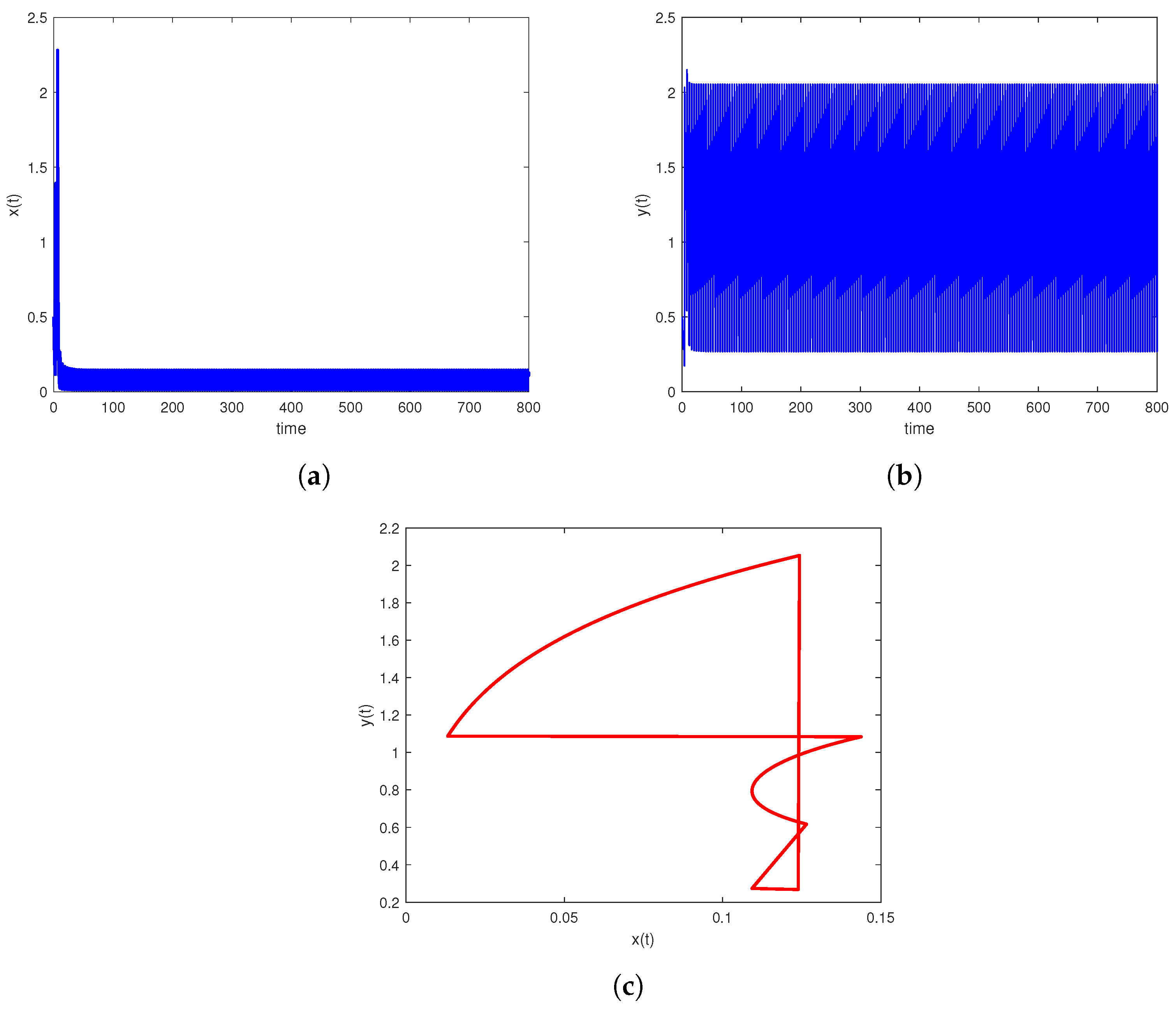
In this paper, we consider a switched IPM model with predation-induced fear and seasonal birth in a pest population. If condition $\left(16\right)$ holds, the pest-eradication solution of system $\left(1\right)$ is found to be GAS. If $\left(28\right)$ holds, system $\left(1\right)$ is also proven to be permanent. Make a notation as $R_0=ln{\displaystyle \frac{1}{(1+b)(1-h_1)}}+d_1{l}_1\tau +{\displaystyle \frac{(1-e^{-d_2{l}_1\tau })y*}{d_2}}-{\displaystyle \frac{a_1}{d_3}}ln\left({\displaystyle \frac{{\delta }_{1}y**+e^{d_3(l_1+l_2)\tau }}{{\delta }_{1}y**+e^{d_3{l}_1\tau }}}\right)+{\displaystyle \frac{e^{-d_3{l}_1\tau }(1-e^{-d_3{l}_2\tau })y**}{d_3}}-{\displaystyle \frac{a_2}{d_4}}ln\left({\displaystyle \frac{{\delta }_{2}y***+e^{d_4\tau }}{{\delta }_{2}y***+e^{d_4(l_1+l_2)\tau }}}\right)+{\displaystyle \frac{e^{-d_4(l_1+l_2)\tau }(1-e^{-d_4\tau })y***}{d_4}}.$ Choose a series of parameters: $d_1=0.6,d_2=0.3,{\beta }_1=0.3,{\gamma }_1=1.5,k_1=0.75,a_1=2,b_1=1,{\beta }_2=2,{\gamma }_2=0.5,d_3=0.45,k_2=0.4,a_2=1.6,b_2=0.35,{\beta }_3=2.5,{\gamma }_3=1.5,d_4=0.25,k_3=0.55,b=10,l_1=0.55,l_2=0.4,h_1=0.15,h_2=0.55,\theta =0.45,\tau =4,{\mu }_{max}=2,{\delta }_1=0.3,{\delta }_2=1$, $x\left(0^{+}\right)=y\left(0^{+}\right)=0.5,$ and then $R_0=-0.1031<0$, and the system is persistent, as shown in Figure 1.

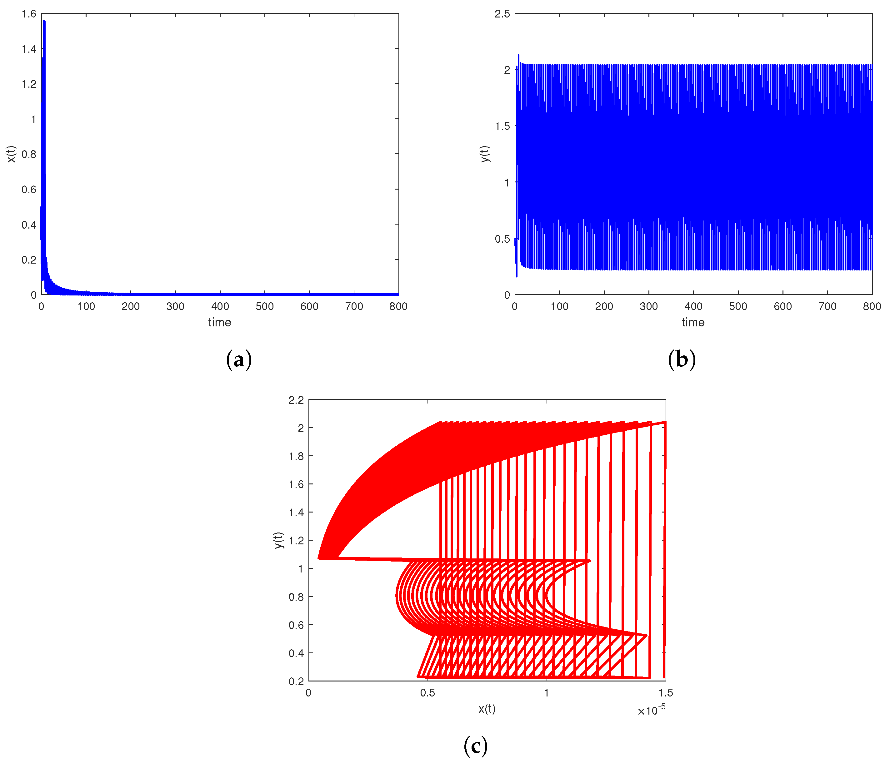
Let $d_1=0.75$, and let the other parameters remain unchanged; then, $R_0=0.2269>0$, and the pest-eradication period solution is locally asymptotically stable (see Figure 2).

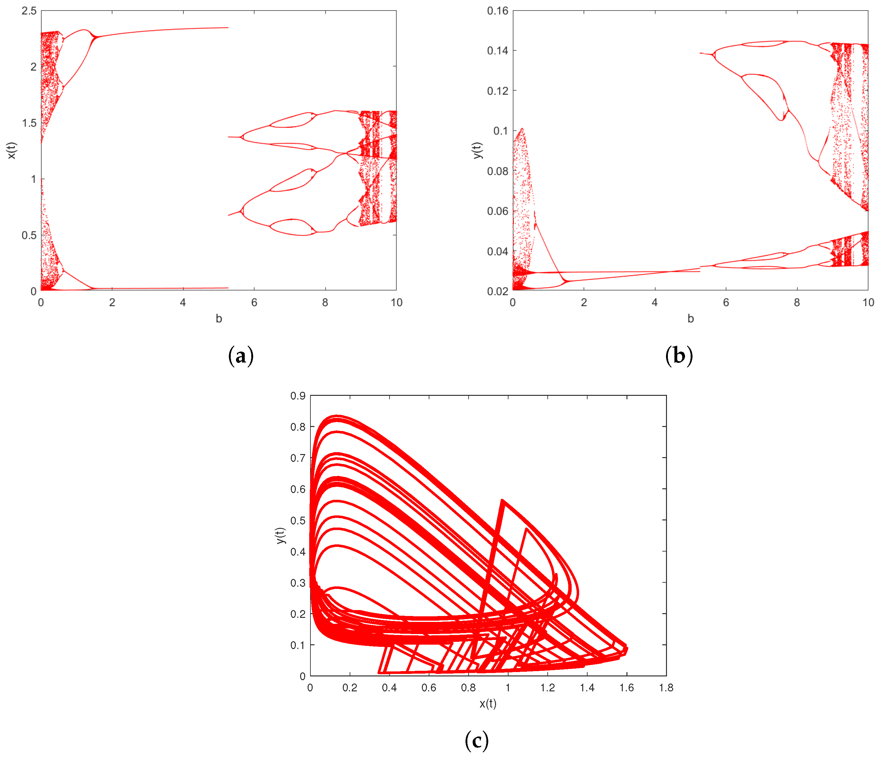
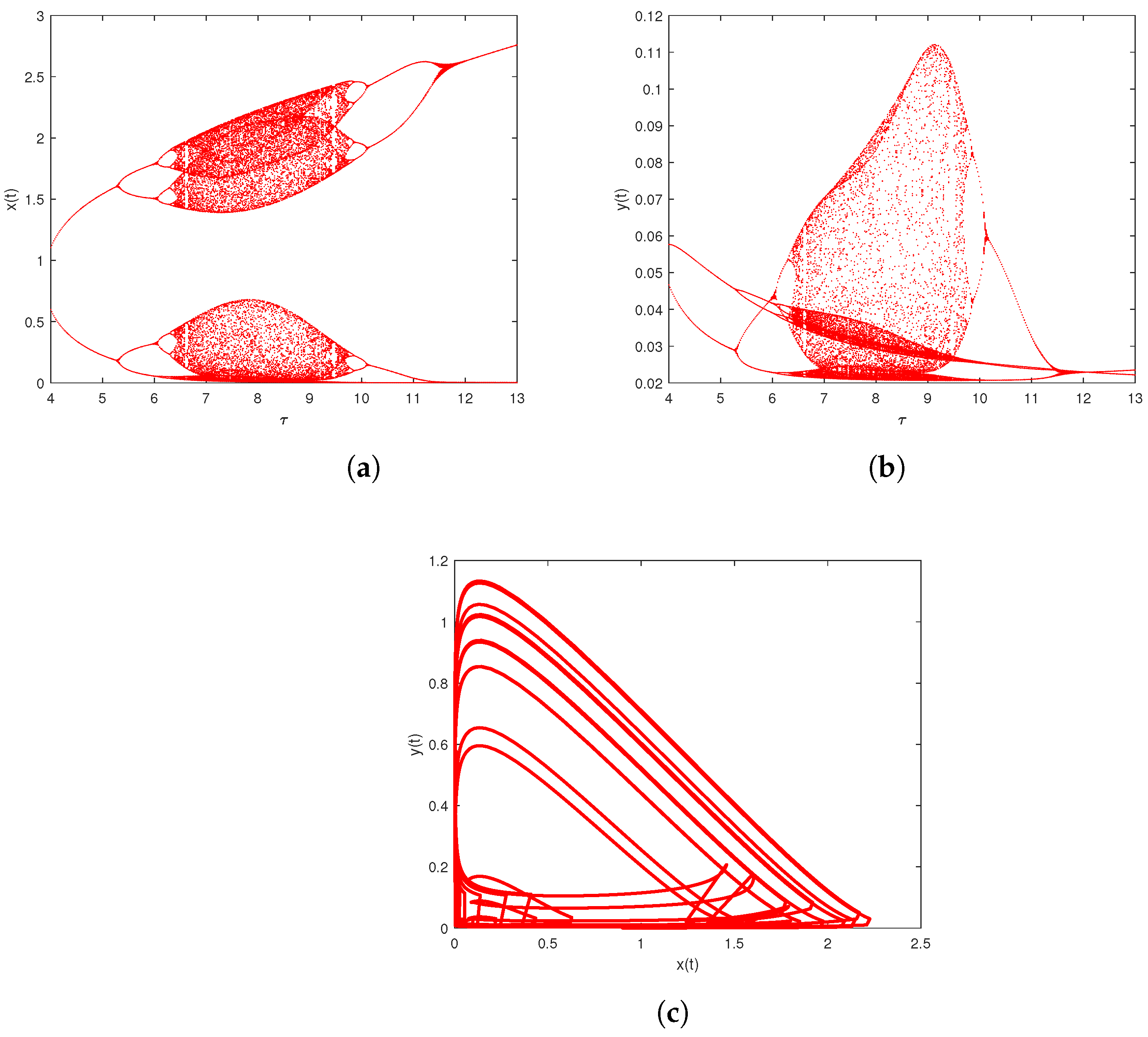
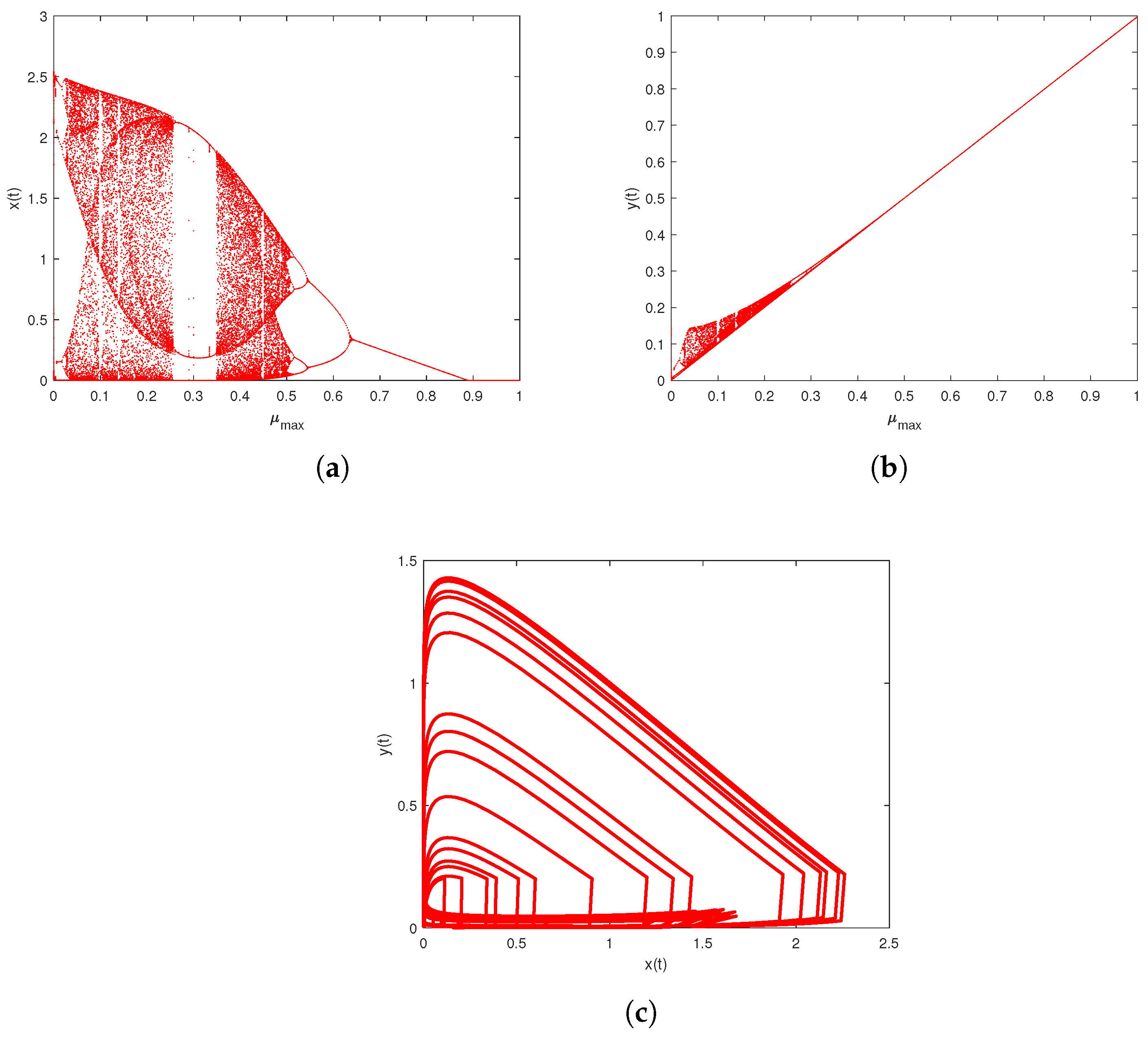
In order to explore more rich dynamical properties, we select some parameters to plot bifurcation graphs. First, we choose parameters as follows: $d_1=0.15,d_2=0.3,{\beta }_1=3,{\gamma }_1=0.02,k_1=0.75,a_1=2,b_1=1,{\beta }_2=2,{\gamma }_2=0.05,d_3=0.45,k_2=0.4,a_2=1.6,b_2=0.35,{\beta }_3=4,{\gamma }_3=0.03,d_4=0.25,k_3=0.55,l_1=0.55,l_2=0.4,h_1=0.15,h_2=0.9,\theta =2,{\mu }_{max}=0.02,\tau =8.5,{\delta }_1=0.3,{\delta }_2=0.4,$ $x\left(0^{+}\right)=y\left(0^{+}\right)=z\left(0^{+}\right)=0.5$, varying b from 0 to 10, and then we obtain the bifurcation parameter graphs versus b (see Figure 3). From these bifurcation graphs of Figure 3, when b increases from a small value to a large value, the pest population changes from chaos to stability, and then multiple periodic solutions appear and finally approach chaos. This result indicates that the pest population will go into eradication while the birth coefficient b is small. So, predation-induced fear will help farmers understand and manage a pest population. Let $b=0.2$, varying $\tau$ from 4 to 13, and let the other parameters remain unchanged; then, the bifurcation parameter graphs versus $\tau$ are as shown in Figure 4. As the bifurcation graph of Figure 4 shows, the birth period $\tau$ increases from a small value to a large value, the pest population changes from stability to chaos and potentially goes into extinction. Let $\tau =10,b=0.2$, varying ${\mu }_{max}$ from 0 to 1; then, we get the bifurcation parameter graphs versus ${\mu }_{max}$, as shown in Figure 5. As the bifurcation graph of Figure 5 shows, impulsively releasing the natural enemy increases ${\mu }_{max}$ from a small value to a large value, and the pest population also changes from stability to chaos and potentially goes to extinction. The analysis tells the farmers that there is a controlling threshold for the amount of the natural enemy to be released.

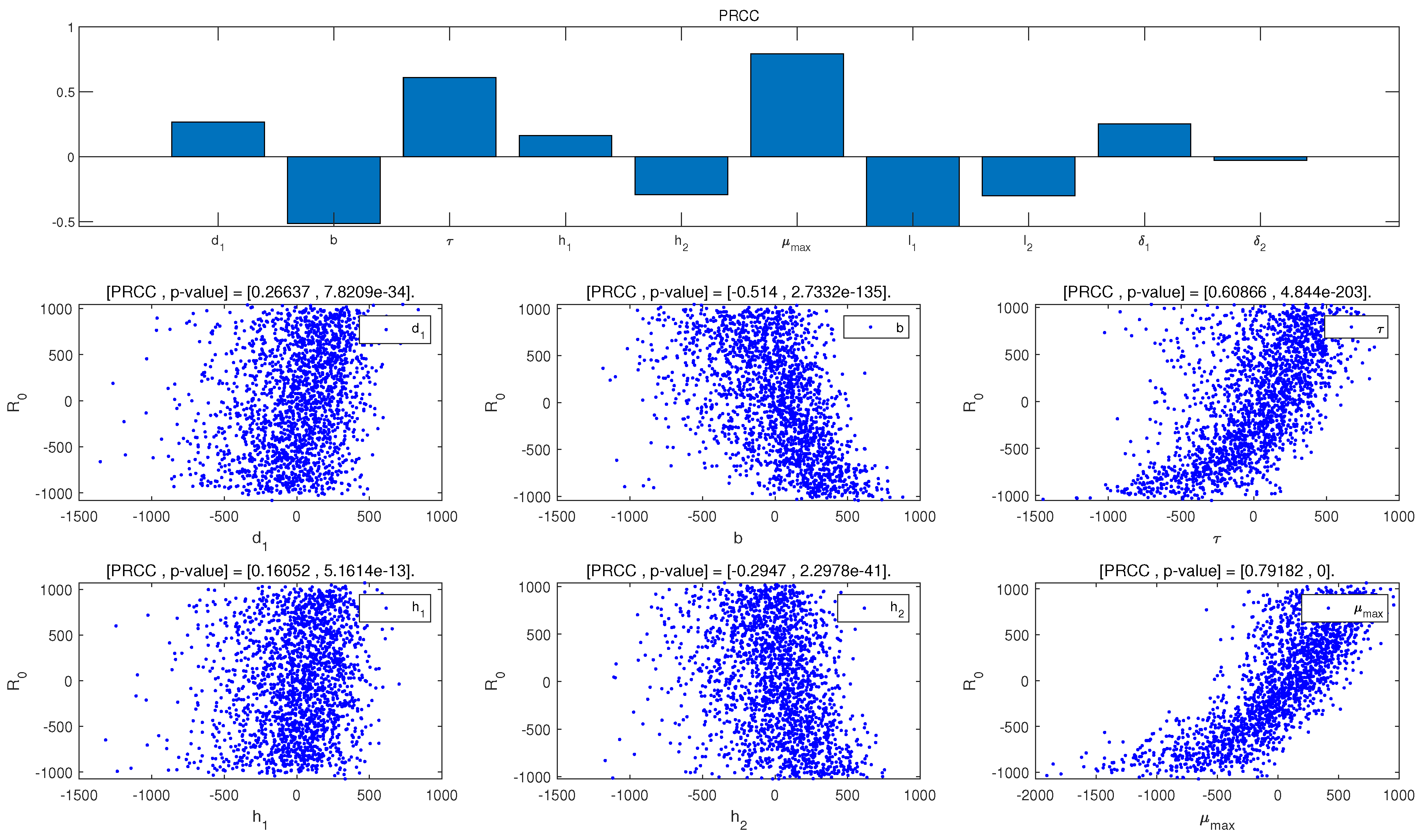
Next, a sensitivity analysis of the parameters is employed to identify the key parameters affecting the pest eradication of system $\left(1\right)$. We choose a series of parameters as baseline values: $d_1=0.65,d_2=0.3,{\beta }_1=0.3,{\gamma }_1=1.5,k_1=0.75,a_1=2,b_1=1,{\beta }_2=2,{\gamma }_2=0.5,d_3=0.45,k_2=0.4,a_2=1.6,b_2=0.35,{\beta }_3=2.5,{\gamma }_3=1.5,d_4=0.25,k_3=0.55,b=10,l_1=0.55,l_2=0.4,h_1=0.15,h_2=0.25,\theta =0.45,\tau =4,{\mu }_{max}=2,{\delta }_1=0.3,{\delta }_2=1$, and then we obtain the sensitivity analysis plot of $R_0$ with respect to some parameters, which are shown in Figure 6. From Figure 6, it can be observed that the birth rate coefficient b, the impulse period $\upsilon$, and $l_1$ have a significant influence on $R_0$.

6. Conclusions

Integrated pest management is very important for crop protection. Our results present appropriate methods for IPM. Although our model is more closely aligned with real-world pest management practices, it can still be further optimized. For example, can we choose to spray pesticides before pests are born? Should refuge be incorporated into these dynamical models? And similar questions can be explored. Moreover, polynomial intervention factors $a\left(t\right),\beta \left(t\right),\delta \left(t\right)$ and $\gamma \left(t\right)$ will replace $a,\beta ,\delta$ and $\gamma$ in the a new correlation model. These will constitute our next works in the future.

References

1. Cullen, J.M.; Sheppard, A.W.; Raghu, S. Effectiveness of classical weed biological control agents released in Australia. Biol. Control 2022, 166, 104835. [Google Scholar] [CrossRef]
2. Moran, V.C.; Hoffmann, J.H.; Zimmermann, H.G. Biological control of invasive alien plants in South Africa: Necessity, circumspection, and success. Front. Ecol. Environ. 2005, 3, 71–77. [Google Scholar] [CrossRef]
3. Chen, L.S.; Chen, J. Nonlinear Biological Dynamic Systems; Scientific Press: Beijing, China, 1993. (In Chinese) [Google Scholar]
4. Chen, L.S. Mathematical Models and Methods in Ecology; Scientific Press: Beijing, China, 1988. (In Chinese) [Google Scholar]
5. Barclay, H.J. Models for pest control using predator release, habitat management and pesticide release in combination. J. Appl. Ecol. 1982, 19, 337–348. [Google Scholar] [CrossRef]
6. Liu, X.N.; Chen, L.S. Complex dynamics of Holling II lotka-volterra predator-prey system with impulsive perturbations on the predator. Chaos Solitons Fractals 2003, 16, 311–320. [Google Scholar] [CrossRef]
7. Byrne, J.; Lillywhite, R.; Creissen, H.; Thorne, F.; Walsh, L. Quantifying integrated pest management adoption in food horticulture. Crop Prot. 2025, 191, 107165. [Google Scholar] [CrossRef]
8. Sanon, A.; De Bauw, P.; Lehmann, E.; Muriuki, L.; Compaoré, I.; Sanou, M.R.; Lopes, T. Development of viable Integrated Pest Management (IPM) strategies to control fall armyworm (Spodoptera frugiperda) on maize. Crop Prot. 2025, 197, 107359. [Google Scholar] [CrossRef]
9. Gopan, A.I.; Ravnskov, S.; Hansen, J.G.; Abuley, I.K. Integrating biological control as a sustainable approach for managing silver scurf and black dot in potatoes. Biol. Control 2026, 212, 105946. [Google Scholar] [CrossRef]
10. Jiao, J.; Chen, L.; Luo, G. An appropriate pest management SI model with biological and chemical control concern. Appl. Math. Comput. 2008, 196, 285–293. [Google Scholar] [CrossRef]
11. Tang, S.; Liang, J.; Tan, Y.; Cheke, R.A. Threshold conditions for integrated pest management models with pesticides that have residual effects. J. Math. Biol. 2004, 66, 1–35. [Google Scholar] [CrossRef] [PubMed]
12. Jiao, J.; Dai, X.; Quan, Q. Dynamics of a pest-nature enemy model for IPM with repeatedly releasing natural enemy and impulsively spraying pesticides. Adv. Contin. Discret. Model. 2025, 52, 1–13. [Google Scholar] [CrossRef]
13. Hobson, K.A.; Wassenaar, L.I. Tracking Animal Migration with Stable Isotopes, 2nd ed.; Academic Press-Elsevier: New York, NY, USA, 2019. [Google Scholar]
14. Quan, Q.; Wang, M.; Jiao, J.; Dai, X. Dynamics of a predator–prey fishery model with birth pulse, impulsive releasing and harvesting on prey. J. Appl. Math. Comput. 2024, 70, 3011–3031. [Google Scholar] [CrossRef]
15. Jiao, J.; Cai, S.; Li, L. Dynamics of a periodic switched predator-prey system with impulsive harvesting and hibernation of prey population. J. Frankl. Inst. 2016, 353, 3818–3834. [Google Scholar] [CrossRef]
16. Jiao, J.J.; Xiao, Y.P. Dynamics of a pest-natural enemy model with natural enemy periodic migration described by time delay. Nonlinear Anal. RWA 2026, 87, 104454. [Google Scholar] [CrossRef]
17. Jiao, J.; Quan, Q.; Dai, X. Dynamics of a new impulsive predator-prey model with predator population seasonally large-scale migration. Appl. Math. Lett. 2022, 132, 108096. [Google Scholar] [CrossRef]
18. Cresswell, W.; Quinn, J.L. Predicting the optimal prey group size from predator hunting behaviour. J. Anim. Ecol. 2011, 80, 310–319. [Google Scholar] [CrossRef]
19. Brown, J.S.; Laundré, J.W.; Gurung, M. The ecology of fear: Optimal foraging, game theory and trophic interactions. J. Mammal. 1999, 80, 385–399. [Google Scholar] [CrossRef]
20. Wang, X.; Zanette, L.; Zou, X. Modelling the fear effect in predator-prey interactions. J. Math. Biol. 2016, 75, 1179–1204. [Google Scholar] [CrossRef] [PubMed]
21. Sahoo, D.; Samanta, G.P. Impact of fear effect in a two prey-one predator system with switching behaviour in predation. Differ. Equ. Dyn. Syst. 2024, 32, 377–399. [Google Scholar] [CrossRef]
22. Hossain, M.; Pal, N.; Samanta, S. Impact of fear on an eco-epidemiological model. Chaos Solitons Fractals 2020, 134, 109718. [Google Scholar] [CrossRef]
23. Lakshmikantham, V. Theory of Impulsive Differential Equations; World Scientific: Singapore, 1989. [Google Scholar]
24. Wu, L.; Jiao, J.; Quan, Q.; Sun, H. Dynamics of a pest management model with nonlinearly impulsive releasing two types of natural enemies and their interspecific cooperation. Chaos Solitons Fractals 2025, 189, 116805. [Google Scholar] [CrossRef]
Figure 1. (a) Time-series of pest x ( t ) with R 0 = 0.1031 < 0 . (b) Time-series of natural enemy y ( t ) with R 0 = 0.1031 < 0 . (c) Persistent phase with R 0 = 0.1031 < 0 .
Axioms 15 00095 g001
Figure 2. (a) Time series of pest x ( t ) with R 0 = 0.2269 > 0 . (b) Time series of natural enemy y ( t ) with R 0 = 0.2269 > 0 . (c) Locally asymptotically stable phase of pest-eradication boundary periodic ( 0 , y ( t ) ¯ ) with R 0 = 0.2269 > 0 .
Axioms 15 00095 g002
Figure 3. (a) Bifurcation graphs versus b of the pest population in system ( 1 ) . (b) Bifurcation graphs versus b of the natural enemy in system ( 1 ) . (c) The chaotic attractor of system ( 1 ) with b = 10 .
Axioms 15 00095 g003
Figure 4. (a) Bifurcation graphs versus τ of the pest population in system ( 1 ) (b) Bifurcation graphs versus τ of the natural enemy in system ( 1 ) . (c) The chaotic attractor of system ( 1 ) with τ = 8 .
Axioms 15 00095 g004
Figure 5. (a) Bifurcation graphs of pest of system ( 1 ) versus μ m a x . (b) Bifurcation graphs of natural enemy of system ( 1 ) versus μ m a x . (c) The chaotic attractor of system ( 1 ) with μ m a x = 0.2 .
Axioms 15 00095 g005
Figure 6. The scatter PRCC value of the threshold R 0 to the key parameters and the scatter plots. The sample size is 2000, and all parameters are varied simultaneously.
Axioms 15 00095 g006