Robust Adaptive Lasso via Robust Sample Autocorrelation Coefficient for the Autoregressive Models

Abstract

For the autoregressive models, classical estimation methods, including the least squares estimator or the maximum likelihood estimator are not robust to heavy-tailed distributions or outliers in the dataset, and lack sparsity, leading to potentially inaccurate estimation and poor generalization capability. Meanwhile, the existing variable selection methods can not handle the case where the influence of explanatory variables on the dependent variable gradually weakens as the lag order increases. To address these issues, we propose a novel robust adaptive lasso method for the autoregressive models. The proposed method is constructed by using partial autocorrelation coefficients as adaptive penalty weights to promote sparsity in parameter estimation, and by employing a robust autocorrelation estimator based on the $F{Q}_n$ statistic to enhance resistance to outliers. Numerical simulations and two real data analyses illustrate the promising performance of our proposed approach. The results indicate that our proposed approach exhibits good robustness and sparsity in the presence of outliers in the dataset.

1. Introduction

Financial market stability is significantly influenced by the prices of the stock index, which serve as crucial indicators of macroeconomic conditions. However, constructing robust and generalizable prediction models for stock indices presents considerable challenges due to their inherent volatility, a characteristic driven by complex interactions among economic, political, cultural and demographic factors. Among various forecasting approaches, time series analysis models, particularly autoregressive (AR) models, have been widely employed for stock price prediction.

Traditional estimation methods for AR models, such as the ordinary least squares (OLS) estimator and the maximum likelihood estimator, perform adequately under some regular conditions, but become unreliable when financial data contain outliers. Such outliers frequently arise from unexpected events such as policy changes, major accidents, and social phenomena. As demonstrated by Box et al. [1], outliers can severely distort time-series model estimates. Two primary approaches have been developed to address this issue: outlier detection and removal, or robust estimation methods that mitigate outlier effects.

In outlier detection research, Huber [2] pioneered methods for identifying outliers in AR models. Chang et al. [3] subsequently extended these methods to ARIMA models with iterative procedures for innovational outliers (IOs) and additive outliers (AOs). Tsay et al. [4] generalized these approaches to multivariate cases, while McQuarrie and Tsai [5] proposed a detection method that does not require prior knowledge of the order, location, or type of the model. Further developments include techniques by Karioti and Caroni [6] for shorter time series and unequal-length AR models, and continuous detection methods introduced by Louni [7] that demonstrate superior performance for IOs. However, most detection methods rely on specific distributional assumptions that are often unrealistic in practice. To address this limitation, Čampulová et al. [8] proposed a nonparametric approach combining data smoothing with change point analysis of residuals.

Compared to outlier detection, robust estimation methods for time series have received less attention. Notable contributions include Pan et al. [9] application of local least absolute deviation for PARMA models and Jiang [10] introduction of exponential square estimators for AR models with heavy-tailed errors. Recent advances by Callens et al. [11] weighted M-estimators with data-driven parameter selection and Chang and Shi [12] reweighted multivariate least trimmed squares and MM-estimators for VAR models.

Traditional time series estimation methods also suffer from poor generalization due to the lack of sparsity. This issue was addressed by the least absolute shrinkage and selection operator (lasso) method [13], which produces sparse and interpretable models. Subsequent developments include smoothly clipped absolute deviation (SCAD) penalty [14] and adaptive lasso [15] to overcome the bias of the lasso method. For AR models, Audrino and Camponovo [16] investigated adaptive lasso’s theoretical properties, Songsiri [17] formulated ${\ell }_1$-regularized least squares problems, and Emmert-Streib and Dehmer [18] proposed a two-step lasso approach for vector autoregression with data-driven feature selection. However, traditional AR model estimation methods are sensitive to outliers and can not deal with the case that the influence of explanatory variables on the dependent variable gradually weakens as the lag order increases. In order to overcome this issue, we propose a novel robust adaptive lasso approach that combines the partial autocorrelation coefficient to construct adaptive penalty weights and uses robust autocorrelation coefficients constructed using the $F{Q}_n$ statistic. Both extensive numerical simulations and a real data example demonstrate the validity of our proposed method.

The rest of the paper is organized as follows: In Section 2, we first review traditional estimation methods for AR models, and present our proposed robust adaptive lasso method. In Section 3, we evaluate the finite-sample performance of the proposed method through Monte Carlo simulations and compare it with other methods. In Section 4, we employ the proposed method to analyze two distinct time series: the S&P 500 Index and the USD/CNY exchange rate. We conclude with some remarks in Section 5.

2. Robust Adaptive Lasso for AR Models

2.1. Least Squares Method

The autoregressive models with order p, denoted as AR(p), can be expressed as follows:

$$y_t={\beta }_0+{\beta }_1{y}_{t-1}+\cdots +{\beta }_p{y}_{t-p}+{\epsilon }_t,$$

(1)

where $y_t$ is the dependent variable, $y_{t-1},\dots ,y_{t-p}$ are explanatory variables, $\mathit{\beta }={({\beta }_0,{\beta }_1,\dots ,{\beta }_p)}^T$ are unknown parameters, and ${\epsilon }_t$ is an independent error term with $E{\epsilon }_t=0$. Given n samples, the coefficients in model (1) can be estimated by minimizing the residual sum of squares:

$${\widehat{\mathit{\beta }}}_{ols}=\underset{\beta }{argmin}\sum _{t=p+1}^n{\left(y_t-{\beta }_0-\sum _{k=1}^p{y}_{t-k}{\beta }_k\right)}^2.$$

(2)

However, the least squares method is non-robust and incapable of order selection, and cannot yield sparse solutions.

2.2. Lasso and Adaptive Lasso Methods

Tibshirani [13] proposed a lasso method that simultaneously performs variable selection and parameter estimation by introducing a penalty term to the objective function in (2), which is given as follows:

$${\widehat{\mathit{\beta }}}_{\mathrm{lasso}}=\underset{\beta }{argmin}\left(\sum _{t=p+1}^n{\left(y_t-{\beta }_0-\sum _{k=1}^p{y}_{t-k}{\beta }_k\right)}^2+{\lambda }_1\sum _{k=1}^p\left|{\beta }_k\right|\right),{\lambda }_1\ge 0,$$

(3)

where ${\lambda }_1$ is nonnegative tuning parameter.

However, the lasso method applies uniform penalty coefficients to all features, which results in biased estimates. To address this limitation, Zou [15] proposed the adaptive lasso method, which assigns smaller penalties to larger coefficients and vice versa. The estimation procedure is introduced as follows:

$${\widehat{\mathit{\beta }}}_{\mathrm{adl}}=\underset{\beta }{argmin}\left(\sum _{t=1}^n{\left(y_t-{\beta }_0-\sum _{k=1}^p{y}_{t-k}{\beta }_k\right)}^2+{\lambda }_2\sum _{k=1}^p{\omega }_{k1}\left|{\beta }_k\right|\right),{\lambda }_2\ge 0,$$

(4)

where ${\lambda }_2$ is a nonnegative penalty parameter, ${\omega }_{k1}=1/{\left|{\widehat{\beta }}_k\right|}^{{\delta }_1}$, ${\delta }_1$ is a positive constant, and ${\widehat{\beta }}_k$ is the estimated value of ${\beta }_k$.

2.3. Robust Adaptive Lasso for AR Models

Classical estimation approaches such as the least squares method lack robustness. For the AR $\left(p\right)$ models, the Yule-Walker equations can be expressed as:

$$\begin{array}{cc}\hfill {\rho }_1& ={\beta }_1{\rho }_0+{\beta }_2{\rho }_1+\cdots +{\beta }_p{\rho }_{1-p},\hfill \\ \hfill {\rho }_2& ={\beta }_1{\rho }_1+{\beta }_2{\rho }_0+\cdots +{\beta }_p{\rho }_{2-p},\hfill \\ \hfill & ⋮\hfill \\ \hfill {\rho }_p& ={\beta }_1{\rho }_{p-1}+{\beta }_2{\rho }_{p-2}+\cdots +{\beta }_p{\rho }_0,\hfill \end{array}$$

(5)

where ${\rho }_j$ denotes the j-th order autocorrelation coefficient.

The Yule–Walker equations form a system of linear equations between the sample autocorrelation function and the coefficients. Clearly, robust coefficients can be obtained by deriving robust autocorrelation functions. However, the expression of the sample autocorrelation function for weakly stationary time series contains the sample mean, which is highly sensitive to outliers, resulting in non-robust ${\widehat{\rho }}_k$. Gnanadesikan and Kettenring [19] proposed an alternative definition of the autocorrelation function, which is defined as follows:

$$\rho ={\displaystyle \frac{var\left(U\right)-var\left(V\right)}{var\left(U\right)+var\left(V\right)}},$$

(6)

where

$$\begin{array}{cc}\hfill U& =\left(X/{\sigma }_1+Y/{\sigma }_2\right)/\sqrt{2},\hfill \\ \hfill V& =\left(X/{\sigma }_1-Y/{\sigma }_2\right)/\sqrt{2}\hfill \end{array}$$

with ${\sigma }_1$ and ${\sigma }_2$ being the standard deviations of X and Y, respectively. The correlation coefficient of the sample can be expressed as follows:

$$\widehat{\rho }={\displaystyle \frac{{\widehat{S}}^2\left(U\right)-{\widehat{S}}^2\left(V\right)}{{\widehat{S}}^2\left(U\right)+{\widehat{S}}^2\left(V\right)}},$$

(7)

where ${\widehat{S}}^2\left(U\right)$ and ${\widehat{S}}^2\left(V\right)$ are the sample variance based on the random sample from U and V, respectively, and are the estimators of $var\left(U\right)$ and $var\left(V\right)$, respectively.

Since $\widehat{\rho }$ in (7) involves the sample variance, it inherits non-robustness. Therefore, it is necessary to seek a robust alternative for the estimator of $\rho$. The median absolute deviation (MAD) is a robust estimator of standard deviation, and has a high breakdown point of 0.5, but at the cost of an efficiency of only 0.37. The breakdown point is a global robustness measure from the perspective of resistance to outliers, referring to the maximum proportion of contaminated data that an estimator can tolerate before becoming meaningless [20]. Refs. [21,22] point out that a 50% breakdown point means that the estimator is insensitive to the corruption made by outliers, provided that the outliers constitute less than 50% of the set. Rousseeuw and Croux [23] proposed another robust estimator, the lower quartile of the absolute pairwise differences ($Q_n$), which has a maximum breakdown point of 0.5 and an efficiency of 0.82. However, the $Q_n$ estimator suffers from high computational complexity. Subsequently, Smirnov et al. [24] constructed an M-estimator by matching its influence function to that of the $Q_n$ estimator, thereby maintaining the high asymptotic efficiency of $Q_n$ while avoiding its high computational complexity, resulting in a fast $Q_n$ statistic, denoted as $F{Q}_n$:

$$F{Q}_n\left(x\right)=1.483{\mathrm{MAD}}_n\left(x\right)\left(1-\left(Z_0-\sqrt{n/\sqrt{2}}\right)/Z_2\right),$$

(8)

$$Z_k=\sum _{i=1}^n{u}_i^k{e}^{-u_i^2/2},(k=0,2;i=1,2,\cdots ,n),$$

(9)

where ${\mathrm{MAD}}_n$ is the median absolute deviation and $\mathrm{med}\left(x\right)$ is the median.

In (8), by employing the k-step M-estimation approach, the final estimator inherits the breakdown point of the initial estimator (Rousseeuw and Croux [25]). Therefore, when MAD is selected as the initial estimator, the $F{Q}_n$ also achieves a breakdown point of 0.5. Using $F{Q}_n$ to estimate the sample standard deviation yields robust sample autocorrelation coefficients:

$$\widehat{\rho }={\displaystyle \frac{F{Q}_n^2\left(u\right)-F{Q}_n^2\left(v\right)}{F{Q}_n^2\left(u\right)+F{Q}_n^2\left(v\right)}}.$$

(10)

The Yule–Walker equations establish the relationship between sample autocorrelation coefficients and parameters to be estimated. By obtaining robust autocorrelation coefficients, we can derive robust parameter estimates through the corresponding algorithms. To achieve both robust and sparse results, these robust correlation coefficients are incorporated into the adaptive lasso method to enhance the model’s robustness.

Generally, the influence of explanatory variables on the dependent variable gradually weakens as the lag order increases. We combine the partial autocorrelation coefficient commonly used in time series order determination with the adaptive lasso method to improve the traditional lasso model.

$${\widehat{\mathit{\beta }}}_{ra}=\underset{\beta }{argmin}\left(\sum _{t=p+1}^n{\left({\widehat{\rho }}_t-\sum _{k=1}^p{\widehat{\rho }}_{t-k}{\beta }_k\right)}^2+{\lambda }_3\sum _{k=1}^p{\omega }_{k3}\left|{\beta }_k\right|\right),{\lambda }_3\ge 0,$$

(11)

where

$${\omega }_{k3}={\displaystyle \frac{1}{|{\widehat{\beta }}_k{|}^{{\delta }_2}{\left|{\widehat{\varphi }}_{kk}\right|}^{{\delta }_3}}},{\delta }_2,{\delta }_3>0,$$

(12)

${\widehat{\rho }}_t$ is the t-th order robust autocorrelation coefficient, the k-th order sample partial autocorrelation coefficient ${\widehat{\varphi }}_{kk}$ is computed recursively as follows:

$${\widehat{\varphi }}_{kk}={\displaystyle \frac{{\widehat{\rho }}_k-{\sum }_{j=1}^{k-1}{\widehat{\varphi }}_{k-1,j}{\widehat{\rho }}_{k-j}}{1-{\sum }_{j=1}^{k-1}{\widehat{\varphi }}_{k-1,j}{\widehat{\rho }}_j}},$$

(13)

where ${\widehat{\rho }}_k$ is the k-th order sample autocorrelation coefficient, ${\widehat{\varphi }}_{k-1,j}$ represents the j-th coefficient estimate from the $(k-1)$-th order partial autocorrelation, and the recursion is initialized with ${\widehat{\varphi }}_{11}={\widehat{\rho }}_1$.

3. Simulation Studies

In this section, we investigate the numerical performance of the proposed method using Monte Carlo simulations. We simulated 100 data sets from the following autoregression model (14) with sample sizes $n=200,400$.

$$y_t={\beta }_1{y}_{t-1}+\cdots +{\beta }_{10}{y}_{t-10}+{\epsilon }_t.$$

(14)

The data are generated by the following three scenarios:

• Scenario 1: The coefficients $({\beta }_1,\dots ,{\beta }_5)=(0.45,-0.37,0.28,0.20,0.15)$ with ${\beta }_j=0$ for $j>5$. The error term follows a Gaussian mixture distribution: ${\epsilon }_t\sim (1-\epsilon )N(0,1)+\epsilon N(0,10)$, where the contamination proportion $\epsilon$ takes values $\{0,0.10,0.20\}$.
• Scenario 2: Maintaining the same coefficient as Scenario 1, the error distribution is replaced by ${\epsilon }_t\sim (1-\epsilon )N(0,1)+\epsilon \mathrm{Cauchy}(0,1)$ with $\epsilon \in \{0,0.10,0.20\}$. The Cauchy component introduces extreme outliers due to its heavy-tailed properties.
• Scenario 3: The coefficients $({\beta }_1,\dots ,{\beta }_5)=(0.85,-0.20,0.15,0.10,0.05)$ with ${\beta }_j=0$ for $j>5$. Characteristic root analysis confirms stationarity with a dominant root modulus of 1.031, inducing strong persistence and slow mean reversion typical of economic time series. The error term follows that of Scenario 1.

To demonstrate the advantage of our proposed method, we compare our proposed method (RA-LASSO) with the traditional adaptive lasso method (LS-LASSO) and the ordinary least squares estimation (OLS). Furthermore, the following four criteria were computed to evaluate the finite sample performance:

• TP: The average accuracy rate of parameter estimates over 100 repetitions.
• Size: The average number of non-zero coefficients in the estimation results over 100 repetitions.
• AE: Mean absolute estimation error: ${\sum }_{j=1}^p|{\widehat{\beta }}_{nj}-{\beta }_j|$.
• SE: Root of mean squares estimation error: $\sqrt{{\sum }_{j=1}^p{|{\widehat{\beta }}_{nj}-{\beta }_j|}^2}$.

For RA-LASSO and LS-LASSO, we take ${\delta }_1={\delta }_2={\delta }_3=0.5$. Meanwhile, these methods require the selection of initial values ${\widehat{\beta }}_{\left(k\right)}$ and the tuning parameters ${\lambda }_2,{\lambda }_3$. In this simulation, we use the ordinary least squares estimates as initial values ${\widehat{\beta }}_{\left(k\right)}$, and select the tuning parameters ${\lambda }_2,{\lambda }_3$ by minimizing the following BIC criterion [26]. The BIC criterion is defined as follows:

$$BIC\left(\lambda \right)=log\left(SSE\left({\widehat{\beta }}_{\lambda }\right)\right)+klog\left(n\right)/n,$$

where $SSE\left({\widehat{\beta }}_{\lambda }\right)={\sum }_{i=1}^n{(y_i-{\widehat{y}}_i)}^2/n$, ${\widehat{y}}_i$ denotes the predicted value of $y_i$, and k denotes the number of non-zero coefficients in ${\widehat{\beta }}_{\lambda }$.

The corresponding simulation results are shown in

Table 1. Simulation results for Scenario 1.

n	$\mathit{\epsilon }$	Method	TP	Size	AE	SE
200	0	OLS	0.500	10.00	0.658	0.802
		LS-LASSO	0.820	5.56	0.615	0.768
		RA-LASSO	0.821	5.49	0.665	0.802
	0.1	OLS	0.500	10.00	1.049	1.017
		LS-LASSO	0.752	4.78	1.088	1.040
		RA-LASSO	0.781	5.33	0.889	0.935
	0.2	OLS	0.500	10.00	1.244	1.112
		LS-LASSO	0.674	5.00	1.213	1.100
		RA-LASSO	0.737	5.05	1.029	1.009
400	0	OLS	0.500	10.00	0.447	0.660
		LS-LASSO	0.853	6.35	0.390	0.614
		RA-LASSO	0.922	5.36	0.452	0.655
	0.1	OLS	0.500	10.00	0.982	0.988
		LS-LASSO	0.767	6.43	0.996	0.996
		RA-LASSO	0.856	5.04	0.826	0.902
	0.2	OLS	0.500	10.00	1.148	1.070
		LS-LASSO	0.673	6.81	1.150	1.071
		RA-LASSO	0.804	4.98	0.992	0.993

,

Table 2. Simulation results for Scenario 2.

n	$\mathit{\epsilon }$	Method	TP	Size	AE	SE
200	0	OLS	0.500	10.00	0.654	0.798
		LASSO	0.815	5.81	0.606	0.763
		RA-LASSO	0.807	5.73	0.664	0.801
	0.1	OLS	0.500	10.00	1.297	1.130
		LS-LASSO	0.634	6.10	1.283	1.126
		RA-LASSO	0.771	4.69	0.920	0.946
	0.2	OLS	0.500	10.00	1.423	1.189
		LS-LASSO	0.578	7.04	1.407	1.183
		RA-LASSO	0.735	4.39	1.032	1.009
400	0	OLS	0.500	10.00	0.455	0.668
		LS-LASSO	0.856	6.30	0.423	0.639
		RA-LASSO	0.902	5.20	0.541	0.719
	0.1	OLS	0.500	10.00	1.270	1.111
		LS-LASSO	0.671	7.41	1.276	1.115
		RA-LASSO	0.835	4.29	0.910	0.944
	0.2	OLS	0.500	10.00	1.423	1.190
		LS-LASSO	0.550	8.44	1.420	1.189
		RA-LASSO	0.797	3.93	1.041	1.015

and

Table 3. Simulation results for Scenario 3.

n	$\mathit{\epsilon }$	Method	TP	Size	AE	SE
200	0	OLS	0.500	10.00	0.706	0.831
		LASSO	0.716	3.76	0.566	0.748
		RA-LASSO	0.656	3.90	0.585	0.759
	0.1	OLS	0.500	10.00	1.224	1.102
		LS-LASSO	0.741	5.99	0.994	0.992
		RA-LASSO	0.672	3.92	0.661	0.807
	0.2	OLS	0.500	10.00	1.329	1.149
		LS-LASSO	0.704	6.76	1.158	1.072
		RA-LASSO	0.660	5.44	0.885	0.931
400	0	OLS	0.500	10.00	0.522	0.712
		LS-LASSO	0.744	4.56	0.477	0.683
		RA-LASSO	0.698	3.10	0.505	0.708
	0.1	OLS	0.500	10.00	1.065	1.030
		LS-LASSO	0.744	6.98	0.929	0.961
		RA-LASSO	0.732	3.82	0.560	0.744
	0.2	OLS	0.500	10.00	1.214	1.101
		LS-LASSO	0.678	7.90	1.122	1.057
		RA-LASSO	0.725	4.57	0.754	0.864

. These results reveal the following:

• For Scenario 1, in the absence of contamination ($\epsilon =0$), all methods performed well. As the contamination level $\epsilon$ increases to 0.1 and 0.2, the advantage of the robust method became pronounced. RA-LASSO consistently achieves a higher TP and lower AE and SE compared to the other methods under contamination.
• For Scenario 2, under no contamination ($\epsilon =0$), the performance of all methods is similar. However, even a mild contamination ($\epsilon =0.1$) drastically degrades the performance of OLS and LS-LASSO. RA-LASSO demonstrates relatively robust performance, outperforming the other two methods. Furthermore, the Size metric reveals that LS-LASSO tends to overfit severely under contamination, whereas RA-LASSO effectively controls model complexity, selecting a model size much closer to the true value.
• For Scenario 3, RA-LASSO consistently delivers the highest TP and the lowest estimation errors (AE and SE) under contamination. This confirms that the proposed method remains effective in the presence of both persistent serial correlation and outliers in the innovations.

4. Empirical Analysis

4.1. Application to S&P 500 Index

The closing price reflects the final trading price of a stock for the day. It is widely used as a stable indicator to measure stock performance because it accounts for all price movements during the trading session. We select the closing prices of the S&P 500 Index from 24 September 2020 to 18 February 2021 as our research dataset, as this period witnessed significant market volatility and substantial price fluctuations, making it suitable for empirical analysis.

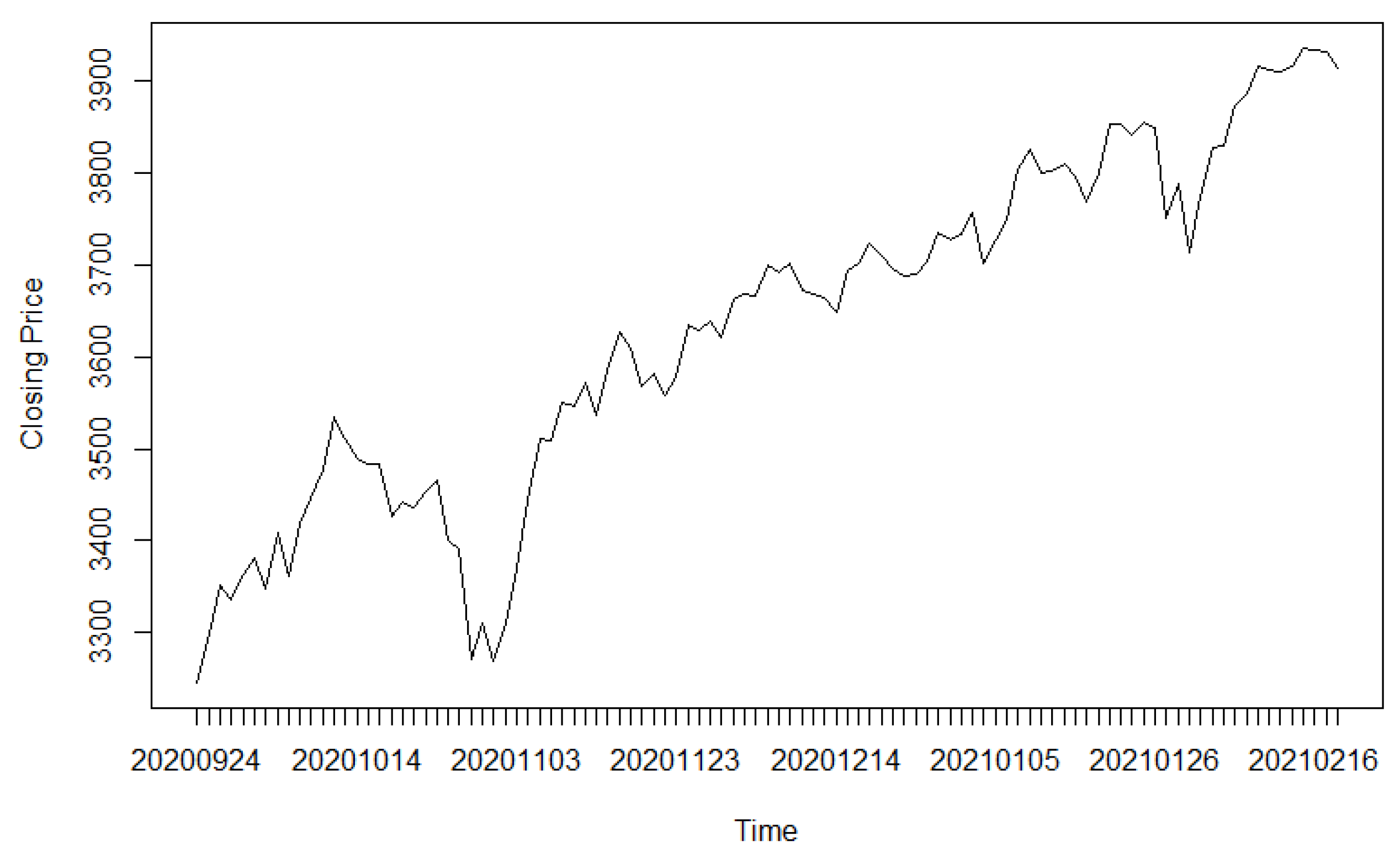
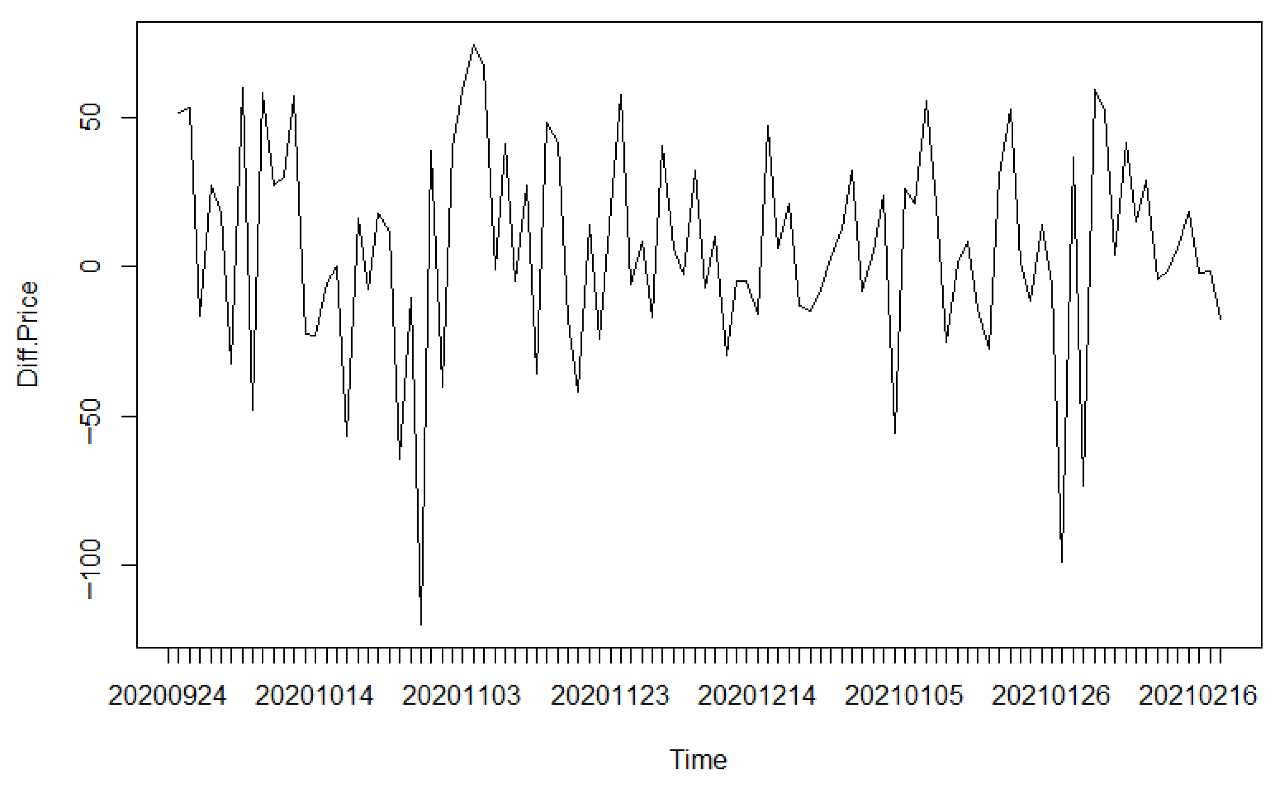
We first plot the closing prices over time in Figure 1, which shows significant fluctuations. To check for stationarity, we performed the augmented Dickey–Fuller (ADF) test. The test results are shown in

Table 4. ADF test results of the S&P 500 daily closing prices.

ADF Test	S&P 500	The First-Differenced S&P 500
Dickey–Fuller	−1.2007	−6.0134
p-value	0.6109	0.01

. From Table 4, we can observe that p-value is 0.6109, which is greater than 0.05, which implies that the series is non-stationary. To address this issue, we take the first-order difference in the closing prices and plot the differenced series in Figure 2. As shown in Figure 2, the differenced series appears more stable, fluctuating randomly around a constant level. Another ADF test on the differenced series (Table 4) yields a p-value of 0.01, confirming stationarity. Although the differenced series is stationary, pronounced outliers are evident in its time series plot. To rigorously diagnose the presence of outliers, we draw a leverage versus standardized residual plot based on a preliminary AR(p) model in Figure 3, where p was determined by the AIC. We can observe from Figure 3 that the absolute values of standardized residuals for three distinct observations exceed the threshold of 2, some even exceeding 3. These extreme values are likely attributable to transient market shocks, such as unexpected earnings reports, geopolitical events, or abrupt changes in investor sentiment, which can introduce significant short-term volatility not eliminated by differencing. Next, we examine the autocorrelation (ACF) and partial autocorrelation (PACF) plots of the differenced series in Figure 4 and Figure 5. Neither the ACF nor the PACF cuts off sharply. Based on Figure 4 and Figure 5, we proceed to fit an AR(p) model to the differenced series.

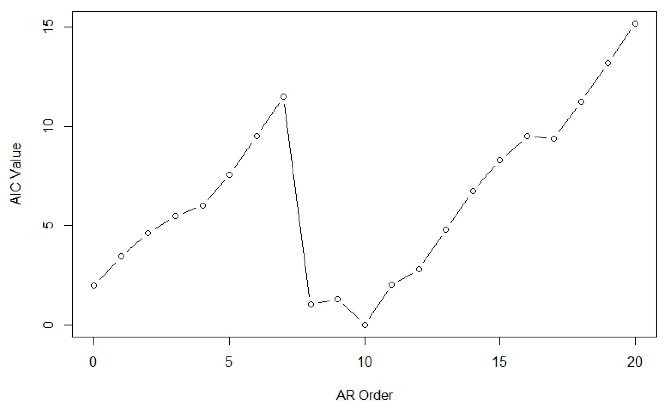
We perform first-order differencing on the closing prices of the S&P 500 Index, denoted as $y_t$, with the p-order lagged differences in daily closing prices denoted as $y_{t-1},\dots ,y_{t-p}$. Firstly, we apply the Akaike information criterion (AIC) to determine the order p for the AR(p) model. Figure 6 presents the AIC values for different model configurations. The results demonstrate that the AIC value reaches its minimum when the lag order is 12. Therefore, we select $p=12$ as the optimal order.

After determining the lag order, we apply the RA-LASSO method, the LS-LASSO method and the OLS method to fit the AR(12) model. The corresponding estimation results are presented in

Table 5. Coefficient estimates comparison of the first-differenced S&P 500 daily closing prices.

Method	$\mathit{t}-$1	$\mathit{t}-$2	$\mathit{t}-$3	$\mathit{t}-$4	$\mathit{t}-$5	$\mathit{t}-$6	$\mathit{t}-$7	$\mathit{t}-$8	$\mathit{t}-$9	$\mathit{t}-$10	$\mathit{t}-$11	$\mathit{t}-$12
OLS	−0.03	0.19	0.07	−0.13	−0.09	−0.23	0.11	0.07	0.10	−0.18	−0.05	−0.22
LS-LASSO	−0.14	0.02	0.16	−0.13	0.00	−0.26	0.09	0.06	0.17	−0.21	−0.17	−0.30
RA-Lasso	−0.04	0.00	0.00	−0.17	0.00	−0.20	0.07	0.00	0.06	−0.16	−0.05	−0.22

. We observe from Table 5 that the number of non-zero elements progressively decreases across the three AR(12) fitted models. The LS-LASSO method selected all lagged days except the $t-$5 day as explanatory variables, the RA-Lasso method selected all lagged days except $t-$2, $t-$3, $t-$5, and $t-$8 days as explanatory variables. Compared with the LS-LASSO method, the RA-Lasso approach demonstrates a faster shrinkage rate and selects fewer variables, indicating superior variable selection performance.

After obtaining the fitted models using three different methods, we further evaluated their prediction accuracy for stock prices. We apply each model to predict the first-order differenced results of the S&P 500 index. The mean absolute percentage error (MAPE) was calculated for each model, defined as follows:

$$\mathrm{MAPE}={\displaystyle \frac{1}{n}}\sum _{i=1}^n\left|{\displaystyle \frac{{\widehat{y}}_i-y_i}{y_i}}\right|,$$

(15)

where $y_i$ represents the actual stock price on day i, and ${\widehat{y}}_i$ denotes the predicted price.

The MAPE results of the three methods are presented in

Table 6. MAPE comparison of the first-differenced S&P 500 daily closing prices.

Method	Size	MAPE
OLS	12	2.12
LS-LASSO	11	2.28
RA-Lasso	8	1.89

. As shown in Table 6, the proposed RA-LASSO method achieves the smallest MAPE, demonstrating its excellent predictive capability.

4.2. Application to USD/CNY Exchange Rate

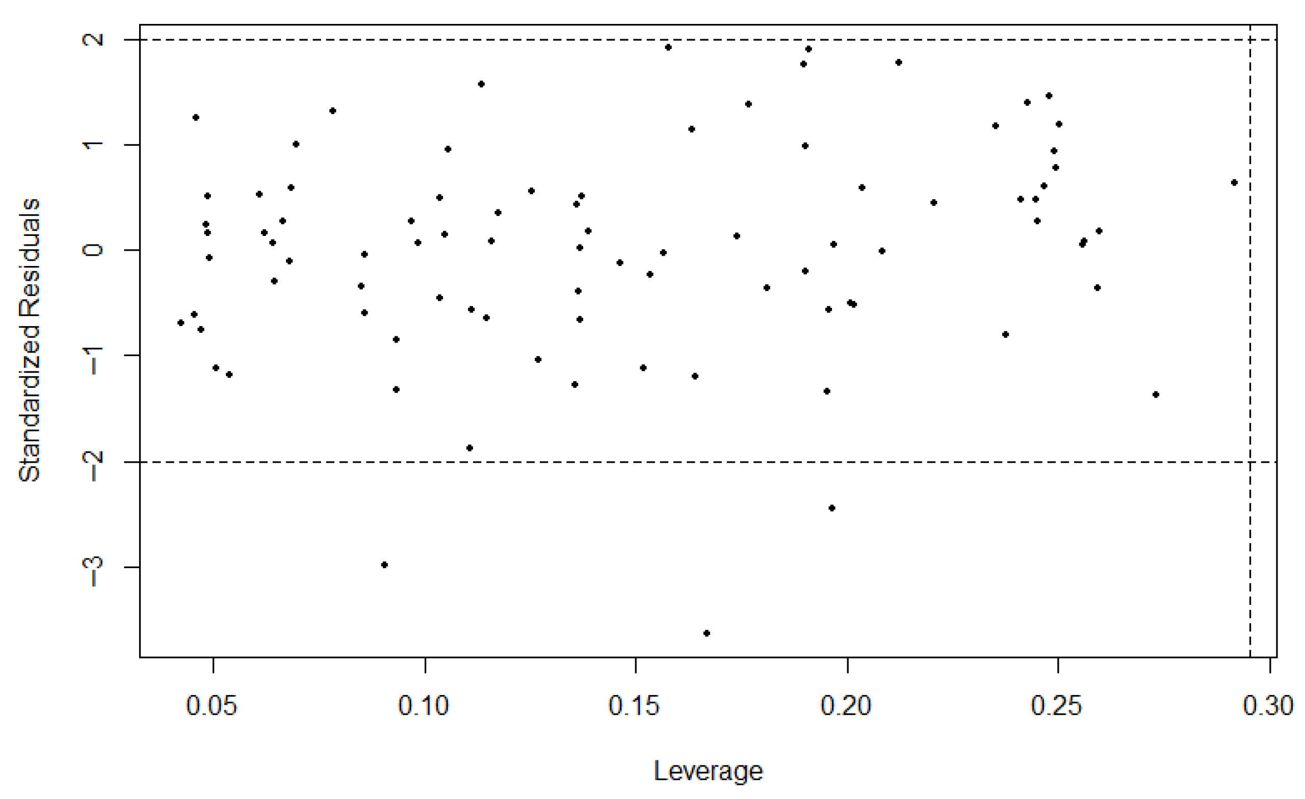
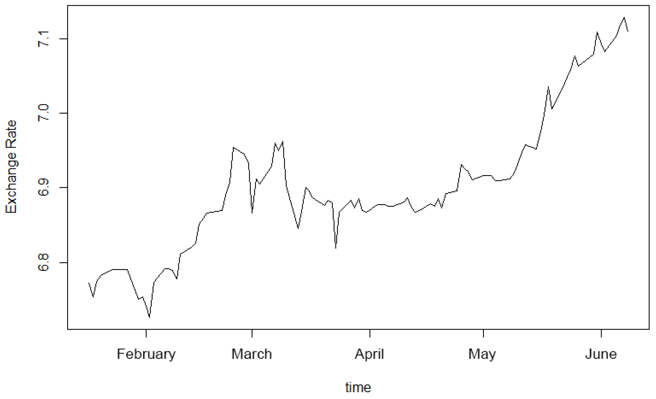
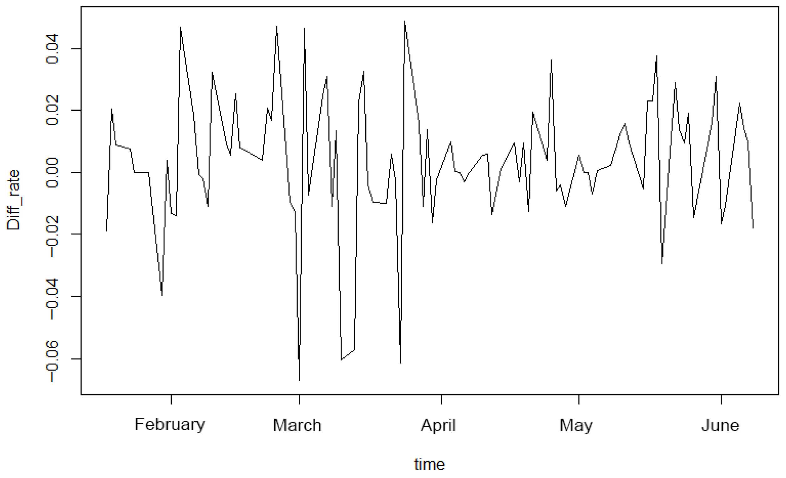
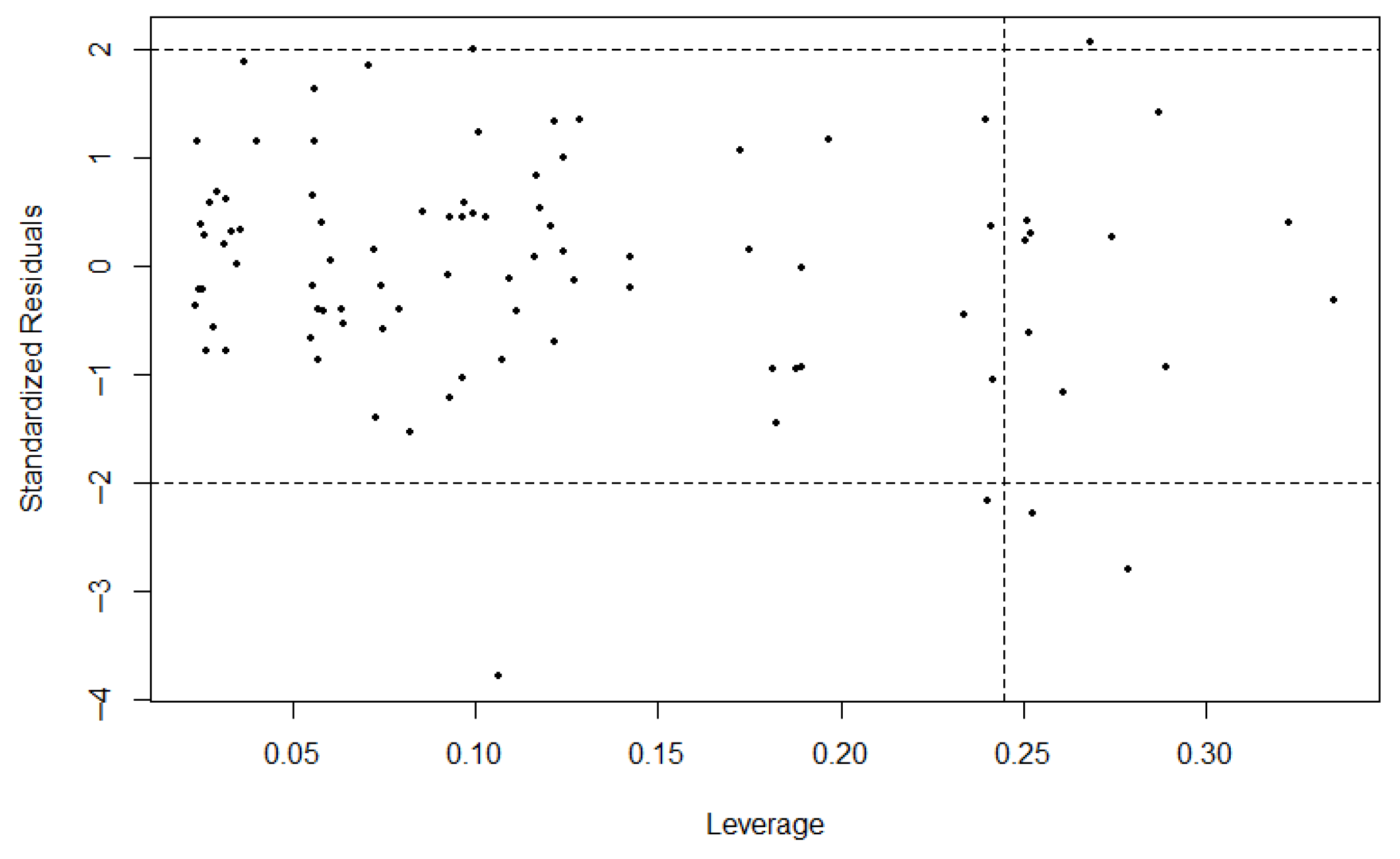
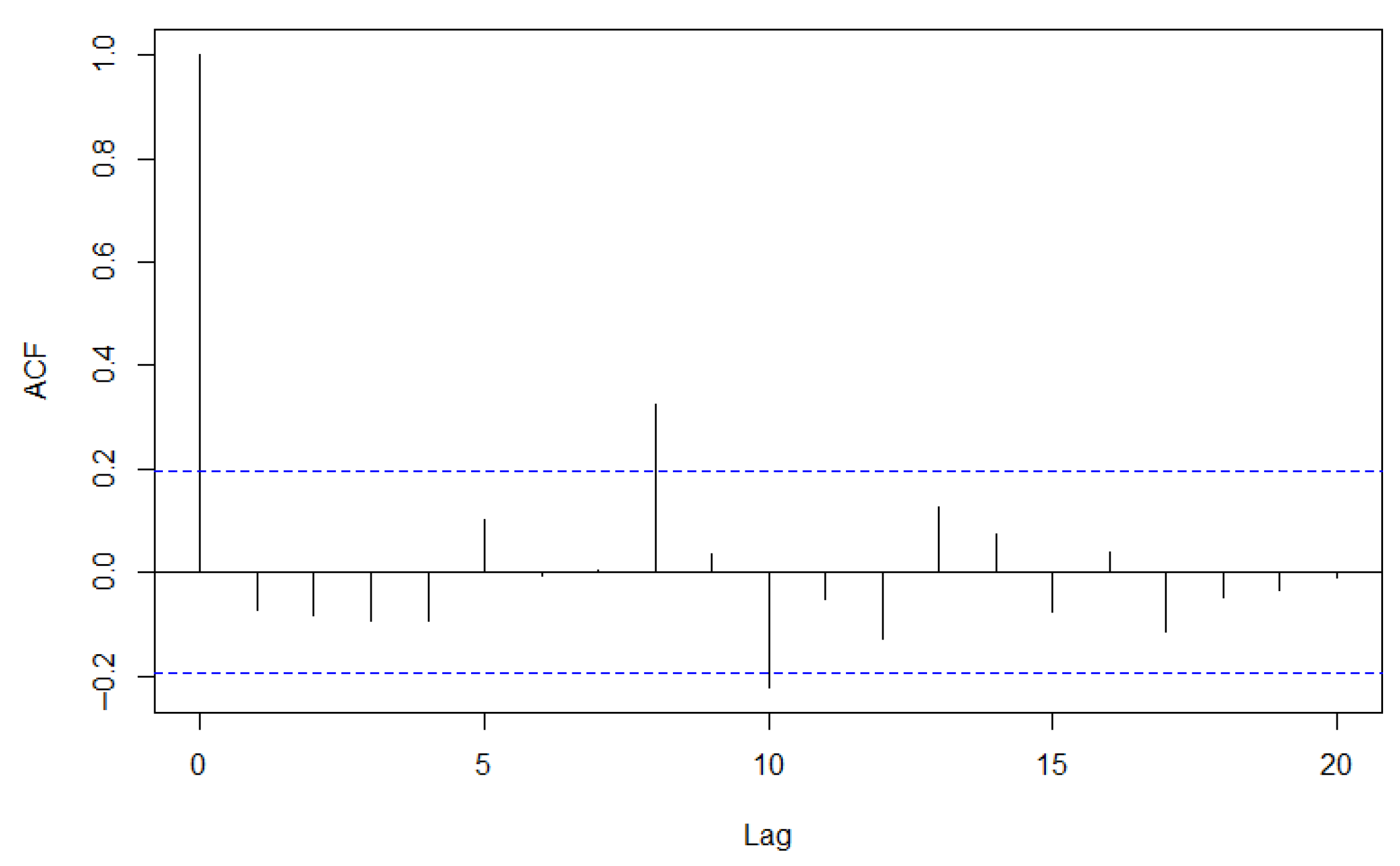
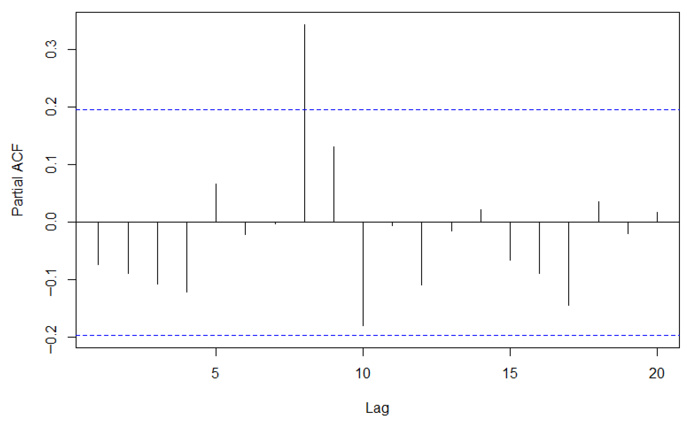
Next, we apply the proposed methodology to analyze the dataset on the exchange rate of the U.S. Dollar against the Chinese Yuan (USD/CNY) from 17 January 2023, to 8 June 2023, sourced from the Federal Reserve Economic Data (FRED) website of the Federal Reserve Bank of St. Louis (fred.stlouisfed.org, accessed on 23 August 2024). During this period, the exchange rate exhibits significant fluctuations. We will utilize these data to compare the robustness of the RA-Lasso method, the LS-Lasso method, and the OLS method. Figure 7 depicts the exchange rate time series, which exhibits considerable variability. An ADF test is conducted to assess stationarity; the results, shown in

Table 7. ADF test results of the USD/CNY exchange rate.

ADF Test	Exchange Rate	The First-Differenced Exchange Rate
Dickey–Fuller	−0.4449	−7.7716
p-value	0.8908	0.01

, yield a p-value of 0.8908, indicating non-stationarity. First-order differencing is applied to achieve stationarity. The differenced series, plotted in Figure 8, appears stable and fluctuates randomly around a constant level. A follow-up ADF test confirms stationarity with a p-value of 0.01. Despite achieving stationarity, the differenced series contains noticeable outliers, likely attributable to transient market disturbances, such as unexpected macroeconomic announcements, geopolitical tensions, or sudden changes in monetary policy expectations. These factors can introduce short-term volatility that differencing alone cannot eliminate. To rigorously diagnose the presence of any outliers and influential points, we employ a leverage versus standardized residual plot (Figure 9) based on a preliminary AR(p) model, where p was determined by the AIC. The plot reveals two distinct phenomena:

• Numerous high-leverage observations, with leverage values exceeding $2\times \overline{h}$, where $\overline{h}$ denotes the mean leverage, indicated by the vertical dashed line.
• Several extreme residuals with absolute standardized values surpassing 2.

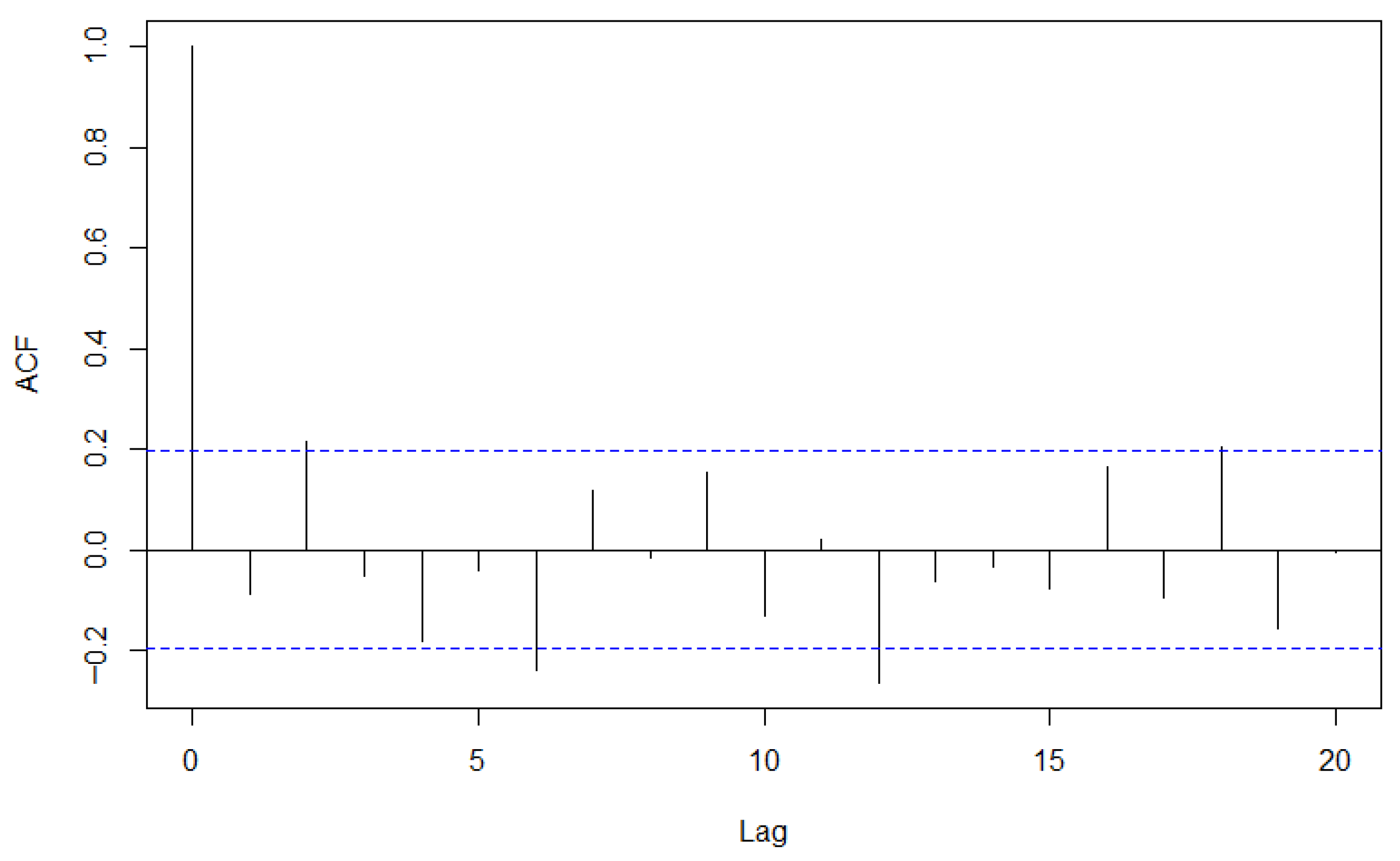
These high-leverage points, predominantly clustered during periods of exceptional market turbulence, may disproportionately influence parameter estimates. The simultaneous presence of large residuals violates the Gaussian error assumption underlying classical estimation methods. The ACF and PACF of the differenced series are presented in Figure 10 and Figure 11. Neither the ACF nor the PACF cuts off sharply.

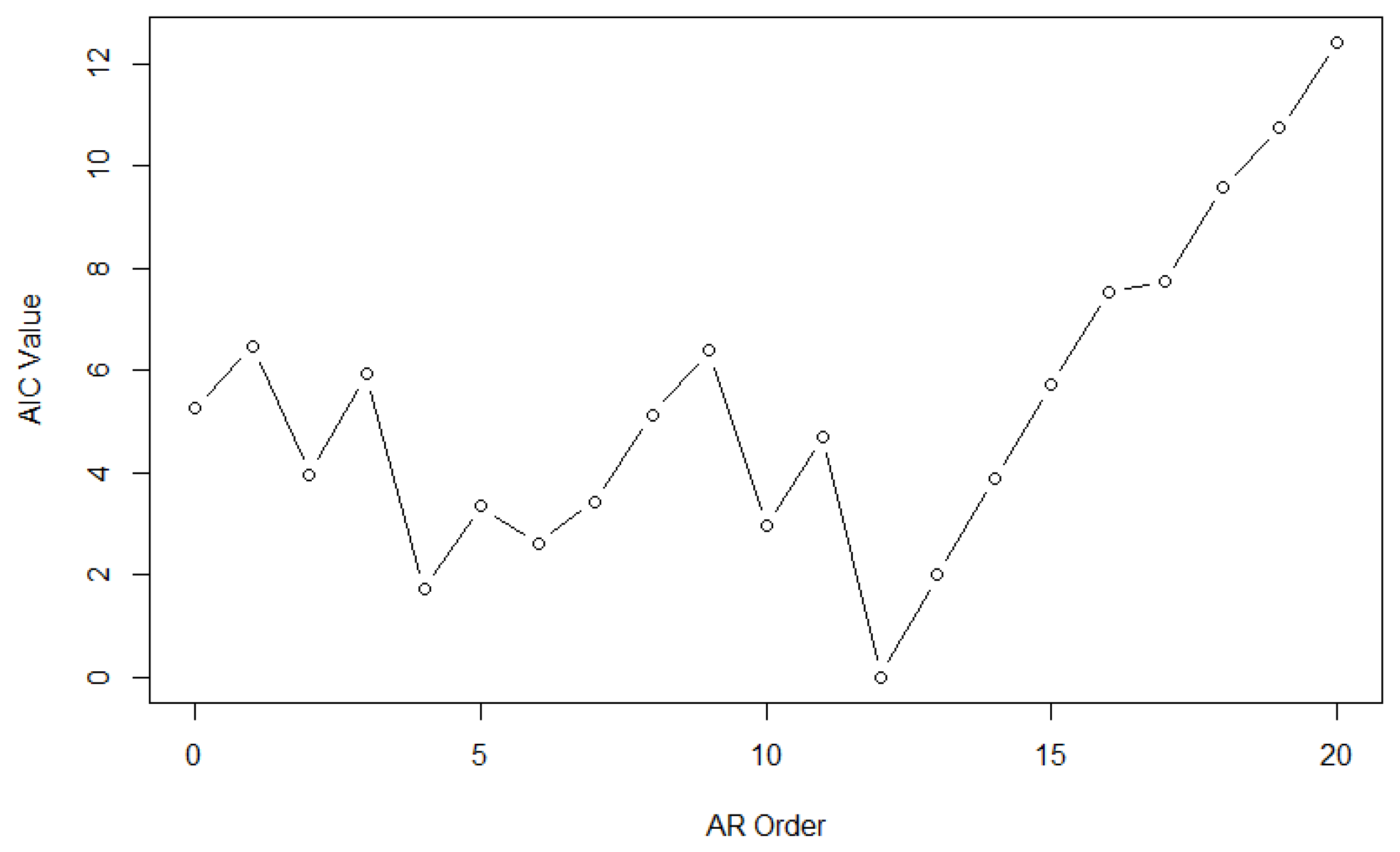
Let $y_t$ represent the first-differenced USD/CNY exchange rate, with $y_{t-1},\dots ,y_{t-p}$ denoting the lagged values. The Akaike Information Criterion (AIC) is used to select the optimal lag order p. As shown in Figure 12, the AIC is minimized at $p=10$, which is selected as the optimal order. The AR(10) model is estimated using RA-LASSO, LS-LASSO, and OLS. Coefficient estimates are reported in

Table 8. Coefficient estimates comparison of the first-differenced USD/CNY exchange rate.

Method	$\mathit{t}-$1	$\mathit{t}-$2	$\mathit{t}-$3	$\mathit{t}-$4	$\mathit{t}-$5	$\mathit{t}-$6	$\mathit{t}-$7	$\mathit{t}-$8	$\mathit{t}-$9	$\mathit{t}-$10
OLS	−0.095	−0.013	−0.095	−0.047	0.184	0.047	0.055	0.373	0.137	−0.187
Lasso	−0.005	−0.069	−0.026	0.079	0.111	0.120	−0.066	0.161	−0.018	−0.152
RA-Lasso	0.000	−0.063	−0.010	0.058	0.101	0.078	0.000	0.157	0.000	−0.132

. The number of non-zero coefficients decreases across methods: LS-LASSO retains all lags, while RA-LASSO further excludes lags $t-1$, $t-7$, and $t-9$. This indicates that RA-LASSO promotes greater sparsity and exhibits a faster shrinkage rate.

Furthermore, the finite sample performance is evaluated using the mean absolute error (MAE) and median absolute deviation (MAD), which are defined as follows:

$$\mathrm{MAE}={\displaystyle \frac{1}{n}}\sum _{i=1}^n\left|{\widehat{y}}_i-y_i\right|$$

(16)

$$\mathrm{MAD}=\mathrm{median}\left(\left|{\widehat{y}}_i-y_i\right|\right)$$

(17)

where $y_i$ denotes the actual exchange rate on the i-th day, and ${\widehat{y}}_i$ represents the predicted exchange rate. The results of the three methods are presented in

Table 9. Result of the first-differenced USD/CNY exchange rate.

Method	Size	MAE	MAD
OLS	10	0.0115	0.0150
LS-LASSO	10	0.0114	0.0151
RA-Lasso	7	0.0111	0.0149

. The proposed RA-LASSO method achieves lower MAE and MAD values than other two methods.

5. Discussion

This paper proposed a robust adaptive lasso method for the autoregressive models by combining the partial autocorrelation coefficient and robust autocorrelation coefficients. Simulation studies and two real data analyses demonstrated that the proposed method had better performance than the existing methods.

It is noteworthy that there are further topics to investigate for our proposed method. Firstly, we will investigate the asymptotic properties of the proposed method as future work. Secondly, we further extend the proposed method to tackle other time series models such as the moving average models and the autoregressive moving average models.

References

1. Box, G.E.; Jenkins, G.M.; Reinsel, G.C.; Ljung, G.M. Time Series Analysis: Forecasting and Control; John Wiley & Sons: Hoboken, NJ, USA, 2015. [Google Scholar]
2. Huber, P.J. The 1972 wald lecture robust statistics: A review. Ann. Math. Stat. 1972, 43, 1041–1067. [Google Scholar] [CrossRef]
3. Chang, I.; Tiao, G.C.; Chen, C. Estimation of time series parameters in the presence of outliers. Technometrics 1988, 30, 193–204. [Google Scholar] [CrossRef]
4. Tsay, R.S.; Pena, D.; Pankratz, A.E. Outliers in multivariate time series. Biometrika 2000, 87, 789–804. [Google Scholar] [CrossRef]
5. McQuarrie, A.D.; Tsai, C.L. Outlier detections in autoregressive models. J. Comput. Graph. Stat. 2003, 12, 450–471. [Google Scholar] [CrossRef]
6. Karioti, V.; Caroni, C. Simple detection of outlying short time series. Stat. Pap. 2004, 45, 267–278. [Google Scholar] [CrossRef]
7. Louni, H. Outlier detection in ARMA models. J. Time Ser. Anal. 2008, 29, 1057–1065. [Google Scholar] [CrossRef]
8. Čampulová, M.; Michálek, J.; Mikuška, P.; Bokal, D. Nonparametric algorithm for identification of outliers in environmental data. J. Chemom. 2018, 32, e2997. [Google Scholar] [CrossRef]
9. Pan, B.; Chen, M.; Wang, Y. Weighted least absolute deviations estimation for periodic ARMA models. Acta Math. Sin. Engl. Ser. 2015, 31, 1273–1288. [Google Scholar] [CrossRef]
10. Jiang, Y. An exponential-squared estimator in the autoregressive model with heavy-tailed errors. Stat. Its Interface 2016, 9, 233–238. [Google Scholar] [CrossRef]
11. Callens, A.; Wang, Y.G.; Fu, L.; Liquet, B. Robust estimation procedure for autoregressive models with heterogeneity. Environ. Model. Assess. 2021, 26, 313–323. [Google Scholar] [CrossRef]
12. Chang, L.; Shi, Y. A discussion on the robust vector autoregressive models: Novel evidence from safe haven assets. Ann. Oper. Res. 2024, 339, 1725–1755. [Google Scholar] [CrossRef]
13. Tibshirani, R. Regression shrinkage and selection via the lasso. J. R. Stat. Soc. Ser. B Stat. Methodol. 1996, 58, 267–288. [Google Scholar] [CrossRef]
14. Fan, J.; Li, R. Variable selection via nonconcave penalized likelihood and its oracle properties. J. Am. Stat. Assoc. 2001, 96, 1348–1360. [Google Scholar] [CrossRef]
15. Zou, H. The adaptive lasso and its oracle properties. J. Am. Stat. Assoc. 2006, 101, 1418–1429. [Google Scholar] [CrossRef]
16. Audrino, F.; Camponovo, L. Oracle properties and finite sample inference of the adaptive lasso for time series regression models. arXiv 2013, arXiv:1312.1473. [Google Scholar] [CrossRef]
17. Songsiri, J. Sparse autoregressive model estimation for learning Granger causality in time series. In Proceedings of the 2013 IEEE International Conference on Acoustics, Speech and Signal Processing, Vancouver, BC, Canada, 26–31 May 2013; pp. 3198–3202. [Google Scholar]
18. Emmert-Streib, F.; Dehmer, M. High-dimensional LASSO-based computational regression models: Regularization, shrinkage, and selection. Mach. Learn. Knowl. Extr. 2019, 1, 359–383. [Google Scholar] [CrossRef]
19. Gnanadesikan, R.; Kettenring, J.R. Robust estimates, residuals, and outlier detection with multiresponse data. Biometrics 1972, 28, 81–124. [Google Scholar] [CrossRef]
20. Donoho, D.L.; Huber, P.J. The notion of breakdown point. In A Festschrift for Erich L. Lehmann; CRC Press: Boca Raton, FL, USA, 1983; Volume 157184. [Google Scholar]
21. Amini, M.; Roozbeh, M. Least trimmed squares ridge estimation in partially linear regression models. J. Stat. Comput. Simul. 2016, 86, 2766–2780. [Google Scholar] [CrossRef]
22. Rousseeuw, P.; Leroy, A. Robust Regression and Outlier Detection; John Wiley & Sons: Hoboken, NJ, USA, 1987. [Google Scholar]
23. Rousseeuw, P.J.; Croux, C. Alternatives to the median absolute deviation. J. Am. Stat. Assoc. 1993, 88, 1273–1283. [Google Scholar] [CrossRef]
24. Smirnov, P.O.; Shevlyakov, G.L.; Smirnov, P.; Smirnov, P.; Shevlyakov, G.; Shevlyakov, G. Approximation of the QN-estimate of scale with the help of fast M-estimates. Sib. Aerosp. J. 2010, 11, 83–85. [Google Scholar]
25. Rousseeuw, P.J.; Croux, C. The bias of k-step M-estimators. Stat. Probab. Lett. 1994, 20, 411–420. [Google Scholar] [CrossRef]
26. Wang, H.; Li, G.; Jiang, G. Robust regression shrinkage and consistent variable selection through the LAD-Lasso. J. Bus. Econ. Stat. 2007, 25, 347–355. [Google Scholar] [CrossRef]
Figure 1. The S&P 500 daily closing price time series plot.
Axioms 14 00701 g001
Figure 2. First-Differenced Series of the S&P 500 daily closing prices.
Axioms 14 00701 g002
Figure 3. Leverage vs. standardized residuals of the first-differenced S&P 500 daily closing prices. The vertical dashed line indicates the threshold of 2 × h ¯ , and the horizontal dashed line marks the ± 2 standard deviation boundaries.
Axioms 14 00701 g003
Figure 4. Sample autocorrelation function of the first-differenced S&P 500 daily closing prices. The blue dotted lines represent the approximate 95% confidence interval.
Axioms 14 00701 g004
Figure 5. Sample partial autocorrelation function of the first-differenced S&P 500 daily closing prices. The blue dotted lines represent the approximate 95% confidence interval.
Axioms 14 00701 g005
Figure 6. The AIC Values for Different Model Configurations of the First-Differenced S&P 500 Daily Closing Prices.
Axioms 14 00701 g006
Figure 7. USD/CNY exchange rate time series plot.
Axioms 14 00701 g007
Figure 8. First-differenced USD/CNY exchange rate.
Axioms 14 00701 g008
Figure 9. Leverage vs. standardized residuals of the first-differenced USD/CNY exchange rate. The vertical dashed line indicates the threshold of 2 × h ¯ , and the horizontal dashed line marks the ± 2 standard deviation boundaries.
Axioms 14 00701 g009
Figure 10. Sample autocorrelation function of the first-differenced USD/CNY exchange rate. The blue dotted lines represent the approximate 95% confidence interval.
Axioms 14 00701 g010
Figure 11. Sample partial autocorrelation function of the first-differenced USD/CNY exchange rate. The blue dotted lines represent the approximate 95% confidence interval.
Axioms 14 00701 g011
Figure 12. The AIC values of the first-differenced USD/CNY exchange rate.
Axioms 14 00701 g012