Derivation of a Closed-Form Asymptotic Variance for the Coefficient of Variation Under the Reparameterized Birnbaum–Saunders Distribution

Abstract

This study develops a tractable, closed-form expression for the asymptotic variance of the coefficient of variation (CV) estimator under a reparameterized Birnbaum–Saunders (BirSau) distribution. Using the method of moments, we derive analytical formulas for the mean, variance, and coefficient of variation of $X\sim \mathrm{BirSau}(\mu ,\lambda )$ and construct a plug-in estimator for the CV. By applying the delta method within this new nonlinear parametrization, we obtain an explicit and compact expression for the asymptotic variance of the CV estimator, thereby extending general asymptotic theory to a distribution-specific setting where higher-order moments lack closed forms under the classical parametrization. Extensive Monte Carlo simulations are conducted to examine the estimator’s finite-sample performance under various parameter configurations and sample sizes. The results demonstrate that the estimator exhibits decreasing bias and variance as the sample size increases, with strong convergence to its theoretical asymptotic behavior. A real-data application using rainfall measurements from northeastern Thailand further illustrates the practical utility of the proposed approach in quantifying relative variability across regions. These findings provide a concise analytical foundation for the coefficient of variation under the Birnbaum–Saunders framework, enhancing its theoretical development and facilitating practical implementation in environmental and reliability analyses.

1. Introduction

The Birnbaum–Saunders (BirSau) distribution, originally introduced by [1], is a flexible model for positively skewed and non-negative data. It has been widely adopted in fields such as reliability engineering, survival analysis, and environmental studies due to its suitability for modeling lifetime and failure-time data [2,3,4]. To ensure accurate inference and model interpretation under the Birnbaum–Saunders distribution, reliable parameter estimation is essential because the accuracy of estimated parameters directly affects the precision of derived quantities such as the mean, variance, and coefficient of variation, as well as the validity of subsequent statistical inferences.

Among the various estimation techniques, the method of moments estimation stands out for its simplicity and analytical tractability. However, the performance of method of moments estimators can be influenced by factors such as sample size and the underlying parameter values, which may result in biased or highly variable estimates in small-sample scenarios. Therefore, studying the asymptotic properties of the estimators of the distribution parameters, namely the shape and scale parameters obtained through the method of moments, is crucial. Understanding their asymptotic behavior allows for the construction of confidence intervals and supports reliable statistical inference for related quantities such as the coefficient of variation [5].

Beyond parameter estimation, the coefficient of variation, defined as the ratio of the standard deviation to the mean, serves as an important scale-free measure of relative variability. It facilitates meaningful comparisons of dispersion across datasets with differing units or magnitudes, making it especially useful in fields such as hydrology, finance, and materials science. However, despite the Birnbaum–Saunders distribution’s extensive applications, the statistical behavior of the CV estimator—particularly under the reparameterized BirSau model—has not been analytically characterized in closed form.

This study addresses this gap by leveraging the reparameterized BirSau model $X\sim \mathrm{BirSau}(\lambda ,\mu )$, in which both the mean and variance are expressed as nonlinear yet analytically tractable functions of the parameters. Using the joint asymptotic distribution of the method of moments estimators and the delta method, we derive a closed-form expression for the asymptotic variance of the CV estimator. This derivation not only extends the general delta-method framework but also provides a distribution-specific formulation that reflects the internal parameter relationships of the BirSau family. Through theoretical analysis, simulation, and real-data validation, we demonstrate that this new formulation allows direct analytical inference for CV without relying on numerical approximation of higher moments. The key contribution of this paper is therefore not to re-establish the asymptotic normality of the CV, but to apply and specialize this general principle to the BirSau distribution by deriving an explicit, closed-form formula for the asymptotic variance of the CV estimator. This formulation offers new theoretical insight into how parameter interactions within the BirSau model shape the behavior of variability measures, and it provides practical tools for statistical inference in reliability and environmental applications.

The article is organized as follows. In Section 2, we provide the overview of results presented in articles [6,7] which are important for our investigation. Section 3 presents the main theoretical result on the asymptotic normality of the CV estimator for the BirSau distribution. An intense simulation study is provided in Section 4, and a real-life example for modeling the total rainfall amounts over consecutive rainy days in northeastern region of Thailand is carefully discussed in Section 6. Section 7 and Section 8 are devoted to a discussion and concluding remarks, respectively.

2. Methodology

This study focuses on analyzing the asymptotic properties of the CV estimator under the parameterization of the BirSau distribution. The methodological framework consists of the following components:

2.1. Parameterization of the Birnbaum–Saunders Distribution

We say that a random variable follows the BirSau distribution (denoted as $X\sim \mathrm{BirSau}(\mu ,\lambda )$, where $\mu >0$ and $\lambda >0$ are the parameters), if its probability density function is given by

$$f(x;\mu ,\lambda )={\displaystyle \frac{1}{2\sqrt{2\pi }}}\left({\displaystyle \frac{\lambda }{x\sqrt{x}}}+{\displaystyle \frac{\mu }{\sqrt{x}}}\right)exp\left\{-{\displaystyle \frac{1}{2}}{\left({\displaystyle \frac{\lambda }{\sqrt{x}}}-\mu \sqrt{x}\right)}^2\right\},x>0.$$

This formulation is referred to as the new parametrization of the BirSau distribution, which differs from the classical parametrization originally introduced by [1]. The advantages of the parametrization are carefully discussed in articles [6,7].

The distribution function for the BirSau$(\lambda ,\mu )$ distribution is

$$F(x;\lambda ,\mu )=\left\{\begin{array}{cc}\hfill \Phi \left(\sqrt{{\displaystyle \frac{x}{\mu }}}-\lambda \sqrt{{\displaystyle \frac{\mu }{x}}}\right),& x>0\hfill \\ \hfill 0,& x\le 0,\hfill \end{array}\right.$$

where $\Phi \left(x\right)$ is the standard normal distribution function. It can be easily shown that the derivative of the distribution function is the density function: ${\displaystyle \frac{dF\left(x\right)}{dx}}=f\left(x\right)$.

The survival function for the BirSau$(\lambda ,\mu )$ distribution is

$$S(x;\lambda ,\mu )=1-F(x;\lambda ,\mu )=\left\{\begin{array}{cc}\hfill 1-\Phi \left(\sqrt{{\displaystyle \frac{x}{\mu }}}-\lambda \sqrt{{\displaystyle \frac{\mu }{x}}}\right),& x>0\hfill \\ \hfill 1,& x\le 0.\hfill \end{array}\right.$$

The hazard rate for the BirSau$(\lambda ,\mu )$ distribution is

$$h\left(x\right)={\displaystyle \frac{f(x;\lambda ,\mu )}{S(x;\lambda ,\mu )}}=\left\{\begin{array}{cc}\hfill {\displaystyle \frac{\frac{1}{2\sqrt{2\pi }}\left(\frac{\lambda }{x\sqrt{x}}+\frac{\mu }{\sqrt{x}}\right)exp\left\{-\frac{1}{2}{\left(\frac{\lambda }{\sqrt{x}}-\mu \sqrt{x}\right)}^2\right\}}{1-\Phi \left(\sqrt{\frac{x}{\mu }}-\lambda \sqrt{\frac{\mu }{x}}\right)}},& x>0\hfill \\ \hfill 0,& x\le 0.\hfill \end{array}\right.$$

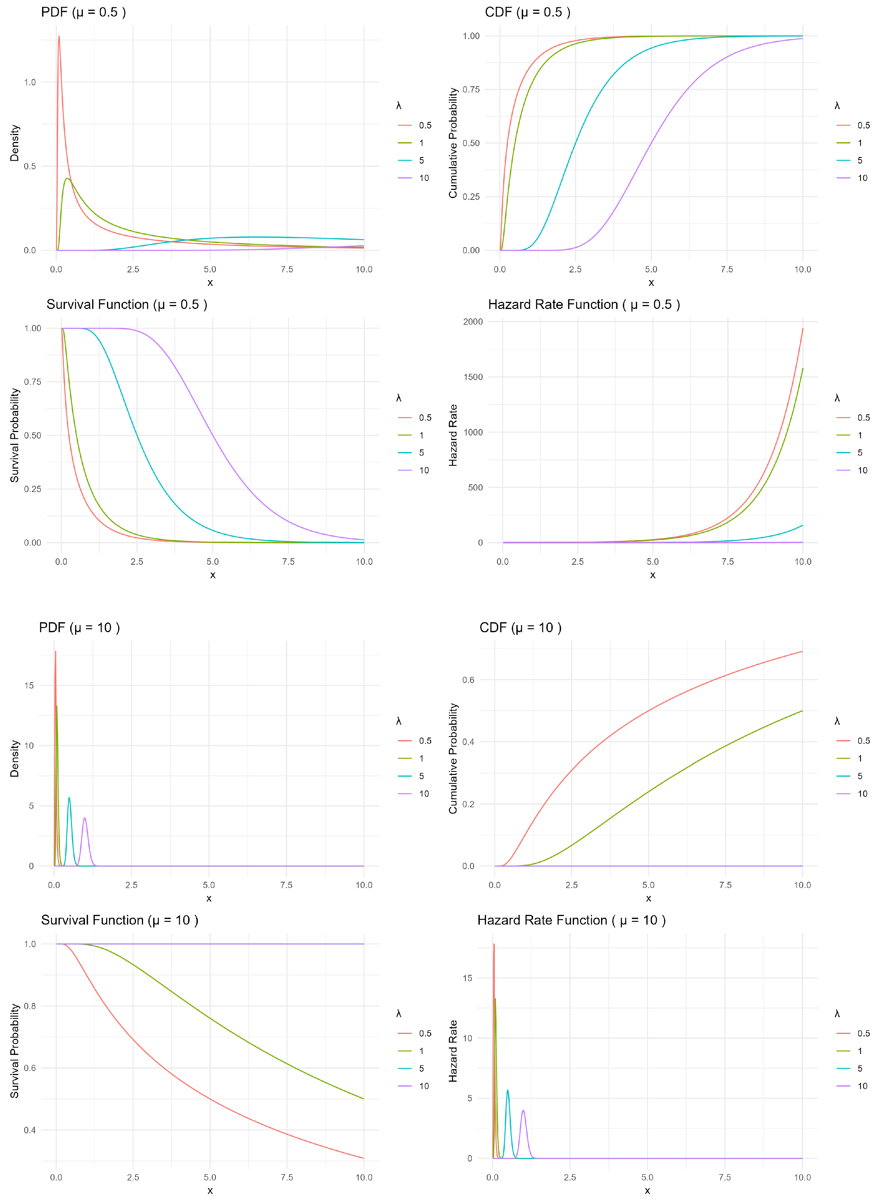
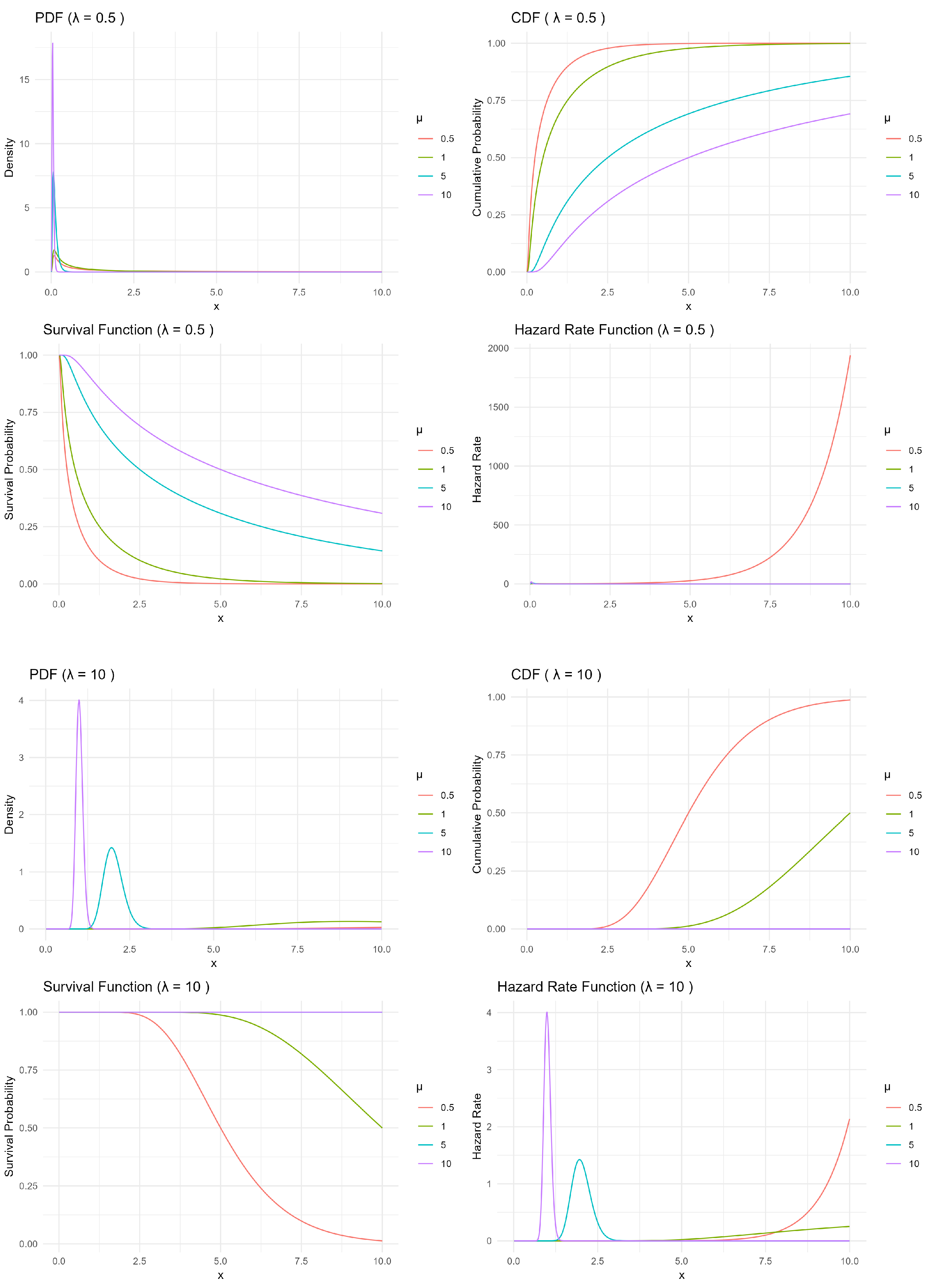
The exact shape of the hazard function (increasing, decreasing, or bathtub-shaped) depends on the values of $\lambda$ and $\mu$. In reliability theory, an increasing hazard rate implies aging (wear-out), a decreasing hazard implies early failure tendency, and a constant hazard suggests a memoryless property. For modeling the total rainfall amounts over consecutive rainy days, the hazard rate function, $h\left(x\right)$, describes the instantaneous risk (or rate) that the total rainfall amount will be around a certain level x, given that it has already exceeded smaller values. An increasing hazard indicates that once a threshold is crossed, the likelihood of even larger rainfall totals becomes greater (heavy-tailed behavior). A decreasing hazard implies that extreme rainfall amounts become less likely as accumulation increases, while a constant hazard suggests that the probability of additional rainfall is independent of the amount already observed. In hydrology, hazard rate functions are often employed to model extreme rainfall events, particularly for assessing flood risk and estimating return periods.

Figure 1 and Figure 2 present the probability density (PDF), cumulative distribution (CDF), survival function (SF), and hazard rate function (HRF) of the Birnbaum–Saunders distribution under different parameter settings, illustrating how variations in $\lambda$ and $\mu$ influence its distributional behavior.

2.2. Method of Moments Estimation of New Parameters

The theoretical background for this section follows Propositions 2 and 3 in [6]. For a random variable $X\sim \mathrm{BirSau}(\lambda ,\mu )$, the mean and variance are given by

$$\mathbb{E}\left(X\right)={\displaystyle \frac{2\lambda \mu +1}{2{\mu }^2}},\mathrm{Var}\left(X\right)={\displaystyle \frac{4\lambda \mu +5}{4{\mu }^4}}.$$

The moment estimators, obtained using the method of moments, are derived by equating the sample moments to the corresponding theoretical moments, yielding the estimators $\widehat{\lambda }$ and $\widehat{\mu }$ as derived in [6,7] .

Furthermore, as established in Theorem 1 of [6], the MMEs are asymptotically normal with mean vector ${(\lambda ,\mu )}^t$ and covariance matrix $\Sigma$; that is,

$$\sqrt{n}\left(\begin{array}{c}\widehat{\lambda }-\lambda \\ \widehat{\mu }-\mu \end{array}\right)⟶N\left(\left(\begin{array}{c}0\\ 0\end{array}\right),\Sigma \right)\mathrm{as}n\to \infty .$$

Full derivations and explicit forms of $\Sigma$ are presented in [6].

3. On the Asymptotic Normality of the CV Estimator for the BirSau Distribution

By the definition, the CV of a random variable X is the ratio of its standard deviation to mathematical expectation $\mathrm{CV}={\displaystyle \frac{\sqrt{\mathrm{Var}\left(X\right)}}{\mathbb{E}\left(X\right)}}$. Taking into consideration the aforementioned formulae for the mean and variance of the BirSau distribution, we establish that if $X\sim \mathrm{BirSau}(\lambda ,\mu )$, then the coefficient of variation is $\mathrm{CV}={\displaystyle \frac{\sqrt{4\lambda \mu +5}}{2\lambda \mu +1}}$.

Therefore, we suggest the following plug-in estimator of the coefficient of variation:

$$\widehat{\mathrm{CV}}={\displaystyle \frac{\sqrt{4\widehat{\lambda }\widehat{\mu }+5}}{2\widehat{\lambda }\widehat{\mu }+1}},$$

(1)

where $\widehat{\lambda }$ and $\widehat{\mu }$ are the moment estimators of the shape and scale parameters of the reparameterized Birnbaum–Saunders distribution, respectively. To find the parameters of the asymptotic normality of the coefficient of variation estimator $\widehat{\mathrm{CV}}$, we apply the famous delta method,; see fundamental monographs [8,9].

Consider two basic statistics $V_1=\widehat{\lambda }$ and $V_2=\widehat{\mu }$. As we already mentioned, random vector ${(V_1,V_2)}^t$ is asymptotically normal with mean ${(\lambda ,\mu )}^t$ and covariance matrix $\Sigma$. Consider function $g(v_1,v_2)={\displaystyle \frac{\sqrt{4v_1{v}_2+5}}{2v_1{v}_2+1}}$. Note that $g(\lambda ,\mu )=\mathrm{CV}$ and $g(V_1,V_2)=g(\widehat{\lambda },\widehat{\mu })=\widehat{\mathrm{CV}}$.

Partial derivatives of the function and their values at the point $(\lambda ,\mu )$ are

$$\begin{array}{cc}\hfill {\displaystyle \frac{\partial g(v_1,v_2)}{\partial v_1}}& ={\displaystyle \frac{8v_2(1-v_1{v}_2)}{\sqrt{4v_1{v}_2+5}{(2v_1{v}_2+1)}^2}},{\displaystyle \frac{\partial g(\lambda ,\mu )}{\partial v_1}}={\displaystyle \frac{8\mu (1-\lambda \mu )}{\sqrt{4\lambda \mu +5}{(2\lambda \mu +1)}^2}},\hfill \\ \hfill {\displaystyle \frac{\partial g(v_1,v_2)}{\partial v_2}}& ={\displaystyle \frac{8v_1(1-v_1{v}_2)}{\sqrt{4v_1{v}_2+5}{(2v_1{v}_2+1)}^2}},{\displaystyle \frac{\partial g(\lambda ,\mu )}{\partial v_2}}={\displaystyle \frac{8\lambda (1-\lambda \mu )}{\sqrt{4\lambda \mu +5}{(2\lambda \mu +1)}^2}}.\hfill \end{array}$$

Therefore, the Taylor expansion of the function $g(v_1,v_2)$ at the point $(\lambda ,\mu )$ up to the linear terms is

$$\begin{array}{cc}\hfill g(v_1,v_2)& =g(\lambda ,\mu )+{\displaystyle \frac{\partial g(\lambda ,\mu )}{\partial v_1}}(v_1-\lambda )+{\displaystyle \frac{\partial g(\lambda ,\mu )}{\partial v_2}}(v_2-\mu )+\mathrm{Remainder}\hfill \\ \hfill & =\mathrm{CV}+{\displaystyle \frac{8(1-\lambda \mu )}{\sqrt{4\lambda \mu +5}{(2\lambda \mu +1)}^2}}(\mu (v_1-\lambda )+\lambda (v_2-\mu ))+\mathrm{Remainder}.\hfill \end{array}$$

Substituting our basic statistics $V_1$ and $V_2$ for variables $v_1$ and $v_2$, we obtain

$$\begin{array}{c}\hfill g(V_1,V_2)=\mathrm{CV}+{\displaystyle \frac{8(1-\lambda \mu )}{\sqrt{4\lambda \mu +5}{(2\lambda \mu +1)}^2}}(\mu (V_1-\lambda )+\lambda (V_2-\mu ))+\mathrm{Remainder}.\end{array}$$

By the delta method, we know that the Remainder converges to zero in probability as the sample size $n\to \infty$. Hence, the estimator $\widehat{\mathrm{CV}}$ has asymptotic mean $\mathrm{CV}$ (asymptotically unbiased) and asymptotic variance

$$\begin{array}{cc}\hfill {\tau }^2& ={\displaystyle \frac{64{(1-\lambda \mu )}^2}{(4\lambda \mu +5){(2\lambda \mu +1)}^4}}\left({\mu }^2\mathrm{Var}\left(\widehat{\lambda }\right)+{\lambda }^2\mathrm{Var}\left(\widehat{\mu }\right)+2\lambda \mu \mathrm{Cov}(\widehat{\lambda },\widehat{\mu })\right)\hfill \\ \hfill & ={\displaystyle \frac{64{(1-\lambda \mu )}^2}{(4\lambda \mu +5){(2\lambda \mu +1)}^4}}\left({\mu }^2{\displaystyle \frac{{\lambda }^2(5+12\lambda \mu +8{\lambda }^2{\mu }^2)}{4{(2\lambda \mu +1)}^2}}+{\lambda }^2{\displaystyle \frac{{\mu }^2(5+12\lambda \mu +8{\lambda }^2{\mu }^2)}{4{(2\lambda \mu +1)}^2}}\right.\hfill \\ \hfill & \left.+2\lambda \mu {\displaystyle \frac{\lambda \mu (-1+4\lambda \mu +8{\lambda }^2{\mu }^2)}{4{(2\lambda \mu +1)}^2}}\right)={\displaystyle \frac{128{\lambda }^2{\mu }^2{(\lambda \mu -1)}^2}{(4\lambda \mu +5){(2\lambda \mu +1)}^4}}.\hfill \end{array}$$

We collect our finding in the following proposition:

Proposition 1. 

The coefficient of variation estimator $\widehat{\mathrm{CV}}={\displaystyle \frac{\sqrt{4\widehat{\lambda }\widehat{\mu }+5}}{2\widehat{\lambda }\widehat{\mu }+1}}$ is asymptotically normal with mean $\mathrm{CV}={\displaystyle \frac{\sqrt{4\lambda \mu +5}}{2\lambda \mu +1}}$ and asymptotic variance

$${\tau }^2={\displaystyle \frac{128{\lambda }^2{\mu }^2{(\lambda \mu -1)}^2}{(4\lambda \mu +5){(2\lambda \mu +1)}^4}};$$

that is,

$$\sqrt{n}(\widehat{\mathrm{CV}}-\mathrm{CV})\to N(0,{\tau }^2)$$

in distribution as $n\to \infty$.

A notable property of this parametrization is its symmetric structure: both parameters $\lambda$ and $\mu$ enter all estimator formulae in an interchangeable manner, such that swapping their roles leaves the expressions unchanged. This elegant symmetry is not preserved in the classical parametrization of the BirSau distribution.

In the following, we consider the following plug-in estimator of the variance ${\tau }^2$:

$${\widehat{\tau }}^2={\displaystyle \frac{128{\widehat{\lambda }}^2{\widehat{\mu }}^2{(\widehat{\lambda }\widehat{\mu }-1)}^2}{(4\widehat{\lambda }\widehat{\mu }+5){(2\widehat{\lambda }\widehat{\mu }+1)}^4}}.$$

The asymptotic $(1-\alpha )$ confidence interval for the CV is $\widehat{\mathrm{CV}}\pm z_{\alpha /2}{\displaystyle \frac{\widehat{\tau }}{\sqrt{n}}}$.

4. Simulation Study

To assess the performance of the proposed estimator of the CV, a Monte Carlo simulation study was conducted. The simulation design is described as follows:

• Sample sizes: $n=10,30,50,100,200,500$,
• Parameter values: $\mu ,\lambda \in \{0.5,1,5,10\}$,
• Number of replications: 10,000 for each combination of $(\mu ,\lambda ,n)$.

The goal is to evaluate the accuracy and reliability of the CV estimator defined by $\widehat{\mathrm{CV}}$.

For each simulation setting, the following performance metrics are computed:

• Bias and mean squared error (MSE) of the CV estimator,
• Empirical standard deviation and sampling distribution of the CV estimator,
• Coverage probabilities of nominal 95% confidence intervals for CV.

The generation procedure for BirSau random variates is discussed in Busababodhin et al. (2025) [6] and can be summarized as follows in Algorithm 1.

Algorithm 1: Generating Birnbaum–Saunders Samples

Fix n, $\mu >0$, and $\lambda >0$. Generate n independent standard normal random variables $y_1,\dots ,y_n$. For each $j=1,\dots ,n$, compute the BirSau random variate $x_j={\left({\displaystyle \frac{-y_j+\sqrt{y_j^2+4\lambda \mu }}{2\mu }}\right)}^2$.

Simulation Procedure for Estimating CV

We apply the following procedure (see Algorithm 2).

Algorithm 2: CV Estimation via Simulation

For each $(\mu ,\lambda ,n)$, repeat the following for $N=10,000$ times: (a) Generate a sample of size n using Algorithm 1. (b) Compute the method of moments estimates ${\widehat{\mu }}_i$, ${\widehat{\lambda }}_i$. (c) Calculate the estimated coefficient of variation ${\widehat{\mathrm{CV}}}_i$ by Equation (1). Compute the following summary statistics over N replications: Bias: $\mathrm{Bias}\left(\widehat{\mathrm{CV}}\right)={\displaystyle \frac{1}{N}}{\sum }_{i=1}^N{\widehat{\mathrm{CV}}}_i-{\mathrm{CV}}_{\mathrm{true}}$. MSE: ${\displaystyle \frac{1}{N}}{\sum }_{i=1}^N{\left({\widehat{\mathrm{CV}}}_i-{\mathrm{CV}}_{\mathrm{true}}\right)}^2$. Empirical standard deviation of $\widehat{\mathrm{CV}}$. Coverage probability of the 95% confidence intervals for CV.

This simulation framework enables comprehensive assessment of the estimator’s performance, especially in terms of the accuracy and robustness of the CV estimation across a wide range of sample sizes and parameter configurations.

5. Comparing the Simulation and Theoretical Results

This section presents a comparative analysis between simulation-based and theoretical results focusing on the estimation of the CV under the BirSau distribution. The analysis emphasizes the accuracy and consistency of the CV estimator by examining its average, variability, and confidence interval performance across different sample sizes and parameter values. Specifically, we evaluate the estimated mean, standard deviation, bias, and MSE of the CV, along with the empirical coverage probability of the 95% confidence interval. The simulation results are organized into three categories based on sample size: small ($n=10,30$), moderate ($n=50,100$), and large ($n=200,500$). For each category, various combinations of the true parameter values $\mu$ and $\lambda$ are considered to assess the robustness of the estimator under diverse distributional conditions. The results provide insight into how the CV estimator converges to its theoretical properties as the sample size increases and offer practical guidance for using CV in applied statistical analysis, especially when sample sizes are limited.

The simulation results for small sample sizes indicate that the coefficient of variation estimator $\widehat{\mathrm{CV}}$ exhibits considerable bias and variability (

Table 1. The simulation and theoretical results for small sample sizes.

n	$\mathit{\lambda }$	$\mathit{\mu }$	CV	Mean $\left(\widehat{\mathbf{CV}}\right)$	Var $\left(\widehat{\mathbf{CV}}\right)$	Bias $\left(\widehat{\mathbf{CV}}\right)$	MSE $\left(\widehat{\mathbf{CV}}\right)$
10	0.5	0.5	1.6330	1.4933	0.0507	−0.1397	0.0702
10	0.5	1	1.3229	1.1914	0.0509	−0.1315	0.0682
10	0.5	5	0.6455	0.5828	0.0202	−0.0627	0.0241
10	0.5	10	0.4545	0.4100	0.0101	−0.0445	0.0121
10	1	0.5	1.3229	1.1930	0.0508	−0.1299	0.0677
10	1	1	1.0000	0.8958	0.0393	−0.1042	0.0502
10	1	5	0.4545	0.4128	0.0102	−0.0418	0.0119
10	1	10	0.3194	0.2898	0.0051	−0.0296	0.0060
10	5	0.5	0.6455	0.5813	0.0198	−0.0642	0.0239
10	5	1	0.4545	0.4114	0.0100	−0.0431	0.0119
10	5	5	0.2009	0.1827	0.0020	−0.0182	0.0023
10	5	10	0.1418	0.1290	0.0010	−0.0127	0.0011
10	10	0.5	0.4545	0.4102	0.0100	−0.0444	0.0120
10	10	1	0.3194	0.2901	0.0050	−0.0294	0.0059
10	10	5	0.1418	0.1282	0.0010	−0.0136	0.0012
10	10	10	0.1001	0.0911	0.0005	−0.0091	0.0006
30	0.5	0.5	1.6330	1.5799	0.0132	−0.0531	0.0161
30	0.5	1	1.3229	1.2705	0.0164	−0.0524	0.0191
30	0.5	5	0.6455	0.6184	0.0069	−0.0271	0.0076
30	0.5	10	0.4545	0.4347	0.0034	−0.0199	0.0038
30	1	0.5	1.3229	1.2705	0.0161	−0.0524	0.0188
30	1	1	1.0000	0.9571	0.0135	−0.0429	0.0154
30	1	5	0.4545	0.4354	0.0034	−0.0191	0.0038
30	1	10	0.3194	0.3062	0.0017	−0.0132	0.0019
30	5	0.5	0.6455	0.6163	0.0070	−0.0292	0.0079
30	5	1	0.4545	0.4347	0.0035	−0.0198	0.0039
30	5	5	0.2009	0.1922	0.0007	−0.0088	0.0007
30	5	10	0.1418	0.1355	0.0003	−0.0063	0.0004
30	10	0.5	0.4545	0.4344	0.0035	−0.0202	0.0039
30	10	1	0.3194	0.3062	0.0017	−0.0133	0.0019
30	10	5	0.1418	0.1357	0.0003	−0.0060	0.0004
30	10	10	0.1001	0.0959	0.0002	−0.0042	0.0002

). Specifically, when $n=10$, the mean estimates of $\widehat{\mathrm{CV}}$ deviate significantly from the true value, and both the bias and MSE are relatively high. These findings suggest that the estimator is not stable or reliable for small samples. Although increasing n from 10 to 30 slightly improves the accuracy, the bias remains non-negligible, and the variance remains substantial. Therefore, $\widehat{\mathrm{CV}}$ should be used cautiously in applications involving small sample sizes.

For moderate sample sizes, the performance of $\widehat{\mathrm{CV}}$ improves considerably (

Table 2. The simulation and theoretical results for moderate sample sizes.

n	$\mathit{\lambda }$	$\mathit{\mu }$	CV	Mean $\left(\widehat{\mathbf{CV}}\right)$	Var $\left(\widehat{\mathbf{CV}}\right)$	Bias $\left(\widehat{\mathbf{CV}}\right)$	MSE $\left(\widehat{\mathbf{CV}}\right)$
50	0.5	0.5	1.6330	1.6114	0.0074	−0.0216	0.0078
50	0.5	1	1.3229	1.3019	0.0095	−0.0210	0.0099
50	0.5	5	0.6455	0.6366	0.0043	−0.0089	0.0043
50	0.5	10	0.4545	0.4473	0.0022	−0.0073	0.0022
50	1	0.5	1.3229	1.3023	0.0094	−0.0205	0.0098
50	1	1	1.0000	0.9842	0.0079	−0.0158	0.0082
50	1	5	0.4545	0.4489	0.0022	−0.0056	0.0022
50	1	10	0.3194	0.3148	0.0010	−0.0046	0.0011
50	5	0.5	0.6455	0.6356	0.0042	−0.0099	0.0043
50	5	1	0.4545	0.4487	0.0022	−0.0058	0.0022
50	5	5	0.2009	0.1983	0.0004	−0.0027	0.0004
50	5	10	0.1418	0.1399	0.0002	−0.0019	0.0002
50	10	0.5	0.4545	0.4478	0.0022	−0.0068	0.0022
50	10	1	0.3194	0.3152	0.0011	−0.0042	0.0011
50	10	5	0.1418	0.1396	0.0002	−0.0021	0.0002
50	10	10	0.1001	0.0987	0.0001	−0.0014	0.0001
100	0.5	0.5	1.6330	1.6232	0.0035	−0.0098	0.0036
100	0.5	1	1.3229	1.3134	0.0047	−0.0095	0.0048
100	0.5	5	0.6455	0.6419	0.0021	−0.0036	0.0021
100	0.5	10	0.4545	0.4523	0.0011	−0.0023	0.0011
100	1	0.5	1.3229	1.3127	0.0046	−0.0102	0.0047
100	1	1	1.0000	0.9921	0.0041	−0.0079	0.0041
100	1	5	0.4545	0.4518	0.0011	−0.0028	0.0011
100	1	10	0.3194	0.3177	0.0005	−0.0017	0.0005
100	5	0.5	0.6455	0.6403	0.0021	−0.0052	0.0022
100	5	1	0.4545	0.4514	0.0011	−0.0031	0.0011
100	5	5	0.2009	0.1999	0.0002	−0.0011	0.0002
100	5	10	0.1418	0.1410	0.0001	−0.0008	0.0001
100	10	0.5	0.4545	0.4516	0.0011	−0.0030	0.0011
100	10	1	0.3194	0.3178	0.0005	−0.0016	0.0005
100	10	5	0.1418	0.1410	0.0001	−0.0008	0.0001
100	10	10	0.1001	0.0995	0.0001	−0.0007	0.0001

). The mean estimates become much closer to the true coefficient of variation, and the bias and MSE decrease notably, particularly when $n=100$. This indicates that the estimator becomes more consistent and unbiased as the sample size increases. The reduced variability and improved precision in this range suggest that moderate sample sizes are generally adequate for reliable inference using $\widehat{\mathrm{CV}}$. These results support the theoretical properties expected from the method of moments under moderate sample conditions.

In large sample settings, the estimator $\widehat{\mathrm{CV}}$ demonstrates excellent performance (

Table 3. The simulation and theoretical results for large sample sizes.

n	$\mathit{\lambda }$	$\mathit{\mu }$	CV	Mean $\left(\widehat{\mathbf{CV}}\right)$	Var $\left(\widehat{\mathbf{CV}}\right)$	Bias $\left(\widehat{\mathbf{CV}}\right)$	MSE $\left(\widehat{\mathbf{CV}}\right)$
200	0.5	0.5	1.6330	1.6342	0.0017	0.0012	0.0017
200	0.5	1	1.3229	1.3256	0.0023	0.0027	0.0023
200	0.5	5	0.6455	0.6482	0.0011	0.0027	0.0011
200	0.5	10	0.4545	0.4558	0.0005	0.0013	0.0005
200	1	0.5	1.3229	1.3247	0.0023	0.0018	0.0023
200	1	1	1.0000	1.0023	0.0020	0.0023	0.0020
200	1	5	0.4545	0.4563	0.0005	0.0018	0.0005
200	1	10	0.3194	0.3207	0.0003	0.0013	0.0003
200	5	0.5	0.6455	0.6480	0.0011	0.0025	0.0011
200	5	1	0.4545	0.4562	0.0005	0.0017	0.0005
200	5	5	0.2009	0.2017	0.0001	0.0008	0.0001
200	5	10	0.1418	0.1424	0.0001	0.0006	0.0001
200	10	0.5	0.4545	0.4564	0.0006	0.0019	0.0006
200	10	1	0.3194	0.3206	0.0003	0.0012	0.0003
200	10	5	0.1418	0.1423	0.0001	0.0005	0.0001
200	10	10	0.1001	0.1005	0.00003	0.0004	0.0000
500	0.5	0.5	1.6330	1.6294	0.0007	−0.0036	0.0007
500	0.5	1	1.3229	1.3192	0.0009	−0.0037	0.0009
500	0.5	5	0.6455	0.6433	0.0004	−0.0022	0.0004
500	0.5	10	0.4545	0.4529	0.0002	−0.0017	0.0002
500	1	0.5	1.3229	1.3191	0.0009	−0.0038	0.0009
500	1	1	1.0000	0.9969	0.0008	−0.0031	0.0008
500	1	5	0.4545	0.4531	0.0002	−0.0014	0.0002
500	1	10	0.3194	0.3185	0.0001	−0.0010	0.0001
500	5	0.5	0.6455	0.6434	0.0004	−0.0021	0.0004
500	5	1	0.4545	0.4530	0.0002	−0.0015	0.0002
500	5	5	0.2009	0.2003	0.00004	−0.0006	0.00004
500	5	10	0.1418	0.1413	0.00002	−0.0004	0.00002
500	10	0.5	0.4545	0.4533	0.0002	−0.0013	0.0002
500	10	1	0.3194	0.3185	0.0001	−0.0009	0.0001
500	10	5	0.1418	0.1413	0.00002	−0.0004	0.00002
500	10	10	0.1001	0.0999	0.00001	−0.0002	0.00001

). The mean estimates are nearly identical to the true coefficient of variation, with bias approaching zero, and both variance and MSE substantially reduced across all parameter settings. These results confirm the asymptotic normality and consistency of the estimator. The precision and stability of $\widehat{\mathrm{CV}}$ in large samples make it highly suitable for practical applications, especially in fields requiring robust statistical inference such as environmental modeling, risk assessment, and decision-support systems.

Across all sample sizes, the estimator $\widehat{\mathrm{CV}}$ shows a clear improvement in performance as the sample size increases. While it is unreliable for small samples due to high bias and variability, its performance improves significantly for moderate samples and becomes highly accurate in large samples. These findings align well with theoretical expectations and support the use of $\widehat{\mathrm{CV}}$ in applications where sufficiently large datasets are available.

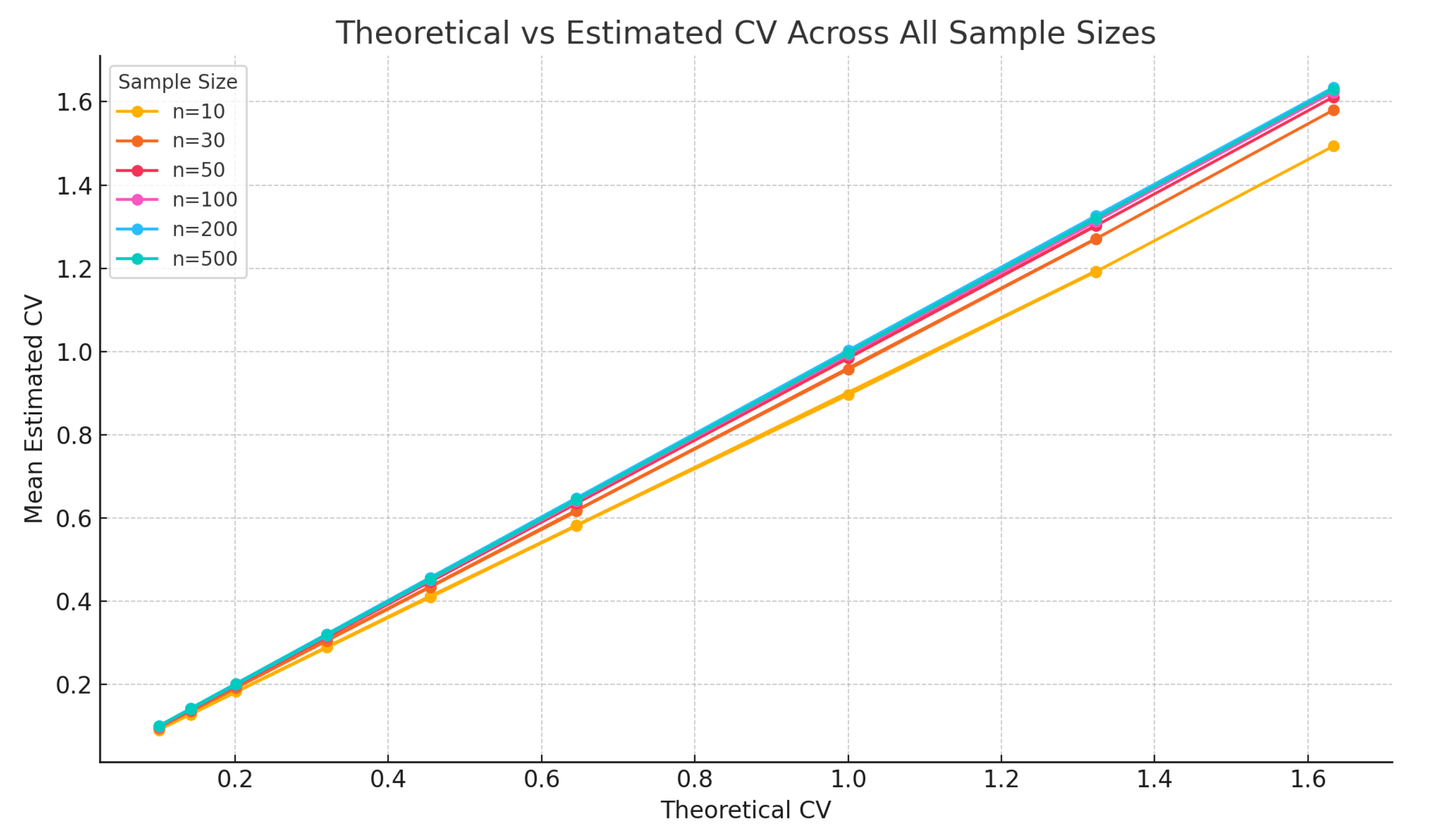
Figure 3 illustrates how the accuracy of the estimated coefficient of variation $\left(\widehat{\mathrm{CV}}\right)$ improves as the sample size increases. The plot compares theoretical CV values with the corresponding simulation-based mean estimates for six different sample sizes: $n=10,30,50,100,200,$ and 500. Each line represents a different sample size and reflects the proximity of the estimated values to their theoretical counterparts.

In small samples ($n=10$ and 30), the estimates exhibit noticeable deviations from the true CV values, revealing substantial bias and variability. As the sample size increases to moderate levels ($n=50$ and 100), the estimates become more accurate and stable. In large samples ($n=200$ and 500), the estimated CVs align almost perfectly with the theoretical values, indicating strong consistency and near-unbiasedness of the estimator.

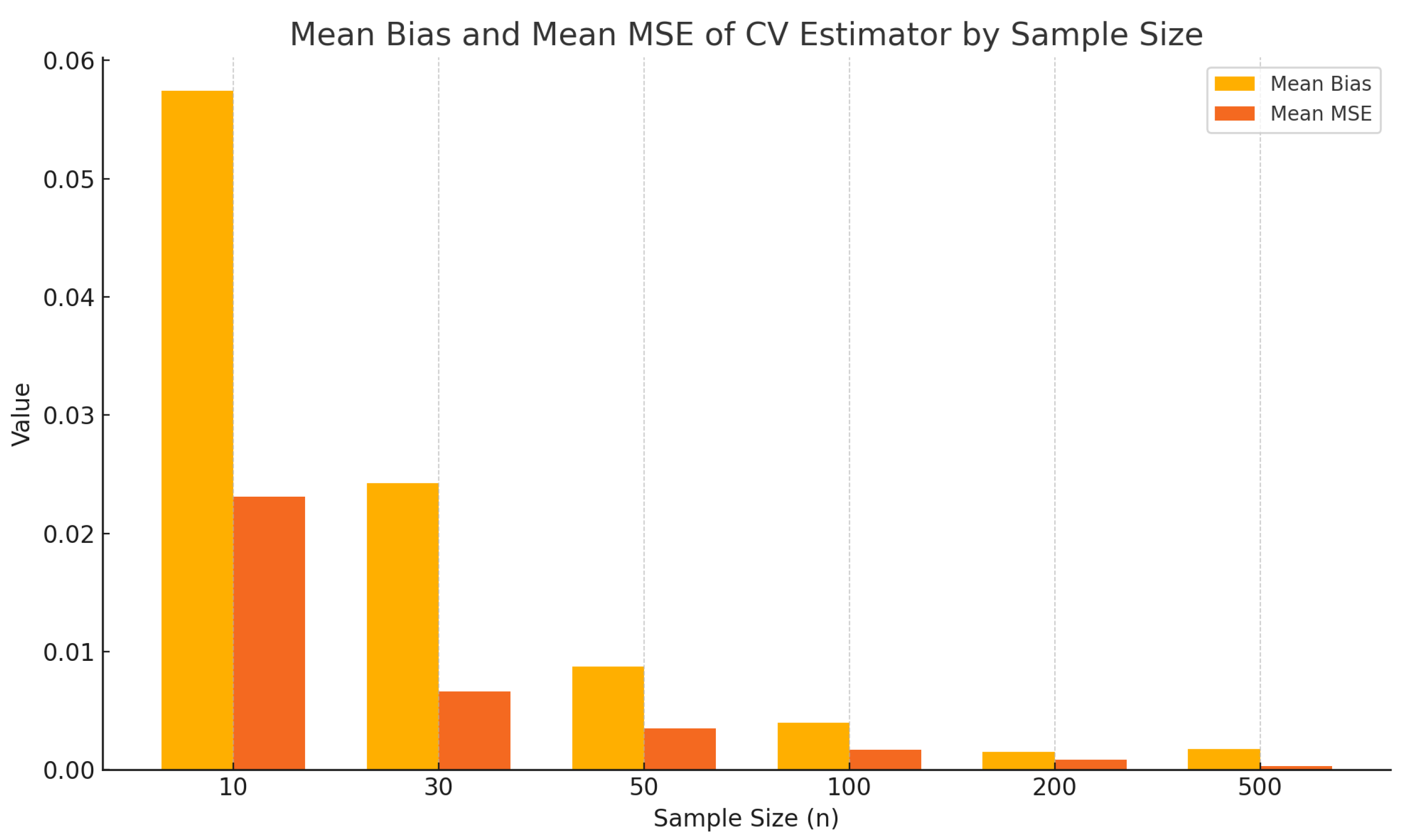
Figure 4 further quantifies this performance by summarizing the mean bias and mean squared error of $\widehat{\mathrm{CV}}$ for each sample size. Both measures decline steadily as the sample size increases, reinforcing the theoretical properties of the method of moments and underscoring the critical role of sufficient sample sizes in achieving reliable inference.

6. Real-Life Example

In Section 5 of the article [6], the applicability of the BirSau distribution to model the total rainfall amounts over consecutive rainy days was demonstrated. The rainfall data from 31 meteorological stations in the northeastern region of Thailand was collected, spanning from January 1984 to September 2024. The suitability of the data for the BirSau distribution was assessed using the Kolmogorov–Smirnov test for goodness-of-fit at a significance level of $\alpha =0.05$. The results indicate that many stations have cumulative rainfall data for consecutive rainy days that align well with the BirSau distribution. 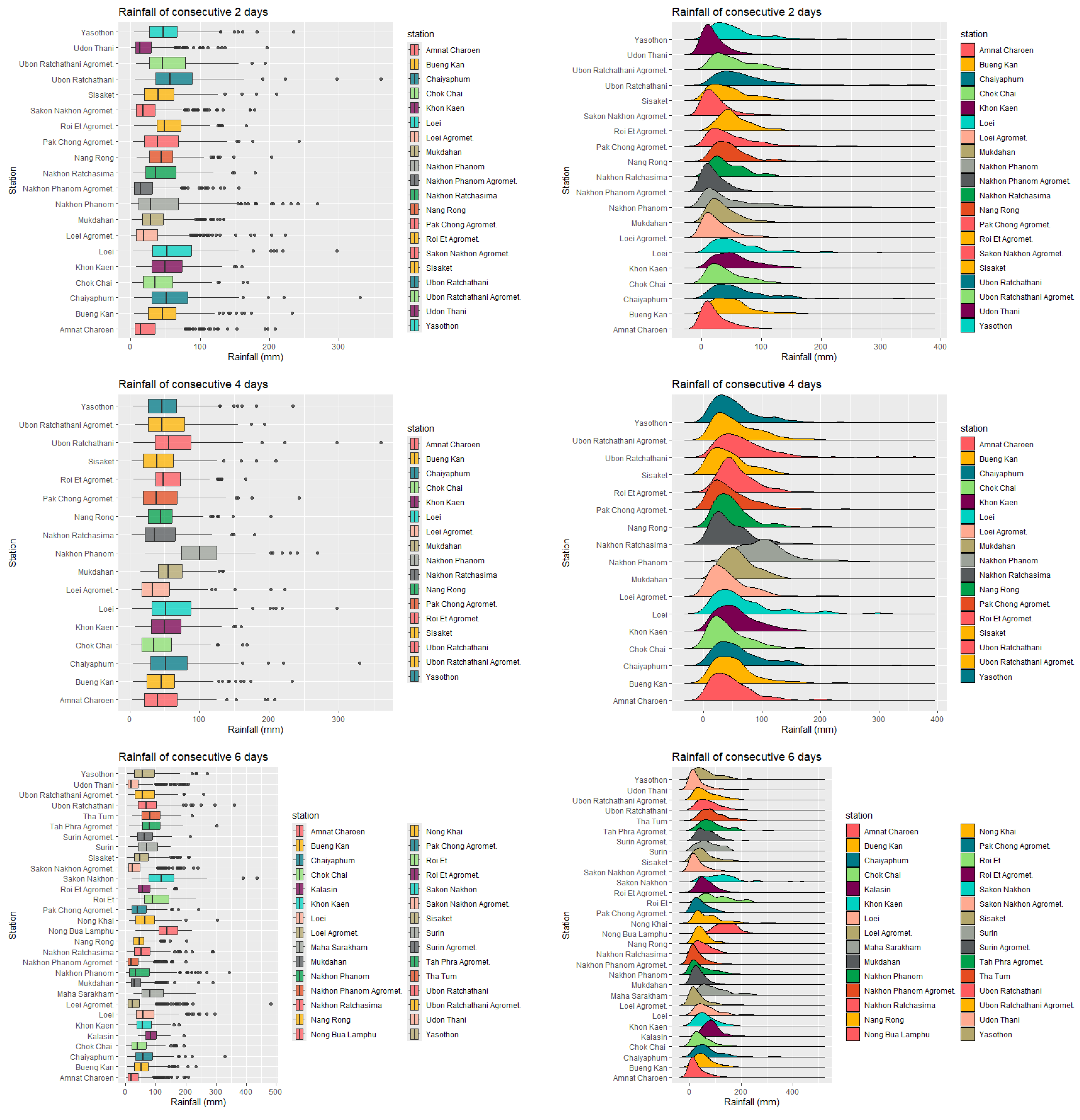Figure 5 presents box plots and density plots for selected stations that passed the goodness-of-fit test for the Birnbaum–Saunders (BirSau) distribution, based on rainfall data aggregated over 2, 4, and 6 consecutive days. Both types of plots reveal that the rainfall distributions are positively skewed, exhibiting pronounced right tails.

CONS-2 to CONS-7 represent different data grouping periods or conditions used in the rainfall analysis, such as time intervals or specific event classifications (

Table 4. Descriptive statistics of rainfall data by station and CONS period.

Data	Station	Min	Mean	Max	sd	Skewness	Kurtosis
CONS-2	Loei Agromet.	0.4	17.41	129.1	17.75	2.14	9.68
	Udon Thani	0.4	20.78	178.5	23.25	2.81	15.27
	Nakhon Phanom	0.4	27.14	178.4	29.99	2.36	9.84
	Nakhon Ratchasima	0.4	19.78	146.2	21.26	2.05	8.58
	Nong Khai	1.9	40.1	193.8	33.63	1.52	5.61
CONS-3	Nakhon Phanom	1.6	40.47	216.8	36.51	2.05	8.66
	Mukdahan	1	39.86	263.5	37.62	2.18	10.02
	Ubon Ratchathani	2.3	43.29	259.4	38.86	2.21	10.5
	Nakhon Ratchasima	0.9	35.44	173.7	31.94	1.89	7.36
CONS-4	Loei Agromet.	2.5	47	230.4	38.91	1.8	7.08
	Nakhon Phanom	3.6	66.74	297.1	53.61	1.72	6.34
	Mukdahan	7.5	56.12	160.4	34.25	0.9	3.38
	Ubon Ratchathani	5	54.95	234.1	41.02	1.54	5.83
	Nakhon Ratchasima	3.3	48.34	210	38.64	1.5	5.81
CONS-5	Loei Agromet.	5.8	65.06	189.5	41.84	0.91	3.19
	Nakhon Phanom Agromet.	12.7	69.76	177.4	34.58	0.89	3.62
	Bueng Kan	36.5	128.72	302.5	55.65	1.01	3.83
	Amnat Charoen	20.9	68.94	146	28.91	0.68	2.98
	Nakhon Ratchasima	4.7	61.07	238.9	44.81	1.77	7.18
CONS-6	Loei Agromet.	12.8	70.96	300.9	46.49	1.96	10.24
	Nakhon Phanom	21.1	128.51	436	81.07	1.65	6.76
	Mukdahan	26.9	92.81	233.5	53.17	0.98	3.3
	Ubon Ratchathani Agromet.	12.6	101.94	270.5	56.29	0.8	3.66
	Nakhon Ratchasima	15.5	83.13	209	50.42	0.9	2.57
CONS-7	Loei Agromet.	23.7	90.34	271.5	51.72	1.62	6.51
	Nakhon Phanom	18.7	125.9	345.7	71.1	0.97	3.96
	Mukdahan	41.5	104.94	194.7	39.61	0.34	2.49
	Ubon Ratchathani Agromet.	22.5	108.63	250.5	54.09	0.49	2.79
	Nakhon Ratchasima	16.2	69.08	196.2	38.07	1.53	6.53

). Each row presents data from meteorological stations located in northeastern Thailand. Variables include Min (minimum), Mean (average), Max (maximum), SD (standard deviation), Skewness (distribution skewness), and Kurtosis (distribution peakedness).

Next, we will apply the theory established in Section 2 for the estimation of the coefficient of variation for the rainfall data. We selected the stations whose total rainfall follows the BirSau distribution and present the asymptotic confidence intervals for the coefficient of variation in

Table 5. 95% confidence intervals for the coefficient of variation for the rainfall data.

Data	Station	n	$\widehat{\mathit{CV}}$	L-Limit (CV)	U-limit (CV)
CONS-2	Loei Agromet.	402	0.2864	0.2761	0.2968
	Udon Thani	358	0.2079	0.2008	0.2150
	Nakhon Phanom	332	0.1733	0.1678	0.1787
	Amnat Charoen	372	0.1002	0.0983	0.1022
	Nakhon Ratchasima	439	0.2294	0.2220	0.2368
CONS-3	Nong Khai	207	1.0579	1.0575	1.0583
	Nakhon Phanom	188	1.1007	1.0995	1.1020
	Mukdahan	204	1.0390	1.0388	1.0392
	Ubon Ratchathani	217	1.0421	1.0419	1.0423
	Nakhon Ratchasima	223	1.1202	1.1186	1.1218
CONS-4	Loei Agromet.	136	0.9420	0.9415	0.9425
	Nakhon Phanom	99	0.8918	0.8898	0.8939
	Mukdahan	113	0.7314	0.7205	0.7423
	Ubon Ratchathani	117	0.8228	0.8178	0.8277
	Nakhon Ratchasima	114	0.9841	0.9841	0.9842
CONS-5	Loei Agromet.	93	0.7848	0.7768	0.7929
	Nakhon Phanom Agromet.	76	0.5433	0.5149	0.5717
	Bueng Kan	83	0.4375	0.4073	0.4676
	Amnat Charoen	88	0.4527	0.4234	0.4819
	Nakhon Ratchasima	69	0.8311	0.8252	0.8370
CONS-6	Loei Agromet.	66	0.7201	0.7048	0.7354
	Nakhon Phanom	55	0.6825	0.6618	0.7032
	Mukdahan	51	0.6006	0.5707	0.6305
	Ubon Ratchathani Agromet.	48	0.6973	0.6769	0.7178
	Nakhon Ratchasima	41	0.6256	0.5950	0.6562
CONS-7	Loei Agromet.	27	0.5560	0.5096	0.6024
	Nakhon Phanom	34	0.6510	0.6206	0.6814
	Mukdahan	33	0.4154	0.3679	0.4629
	Ubon Ratchathani Agromet.	35	0.5974	0.5609	0.6338
	Nakhon Ratchasima	23	0.5805	0.5332	0.6278

. Non-overlapping confidence intervals suggest statistically significant differences in rainfall variability between stations, while overlapping intervals indicate that the variability may be similar. This approach is particularly useful for identifying regions with unusually high or low relative variability, which is important for hydrological planning and resource management.

Figure 5 displays box plots and density plots for rainfall data collected from selected meteorological stations that fit the Birnbaum–Saunders distribution. The box plots summarize the median, interquartile range, and potential outliers (shown as dots), while the density plots show the probability distribution of rainfall amounts. The results clearly indicate right-skewed rainfall distributions, consistent with the BirSau model’s ability to describe positively skewed environmental data.

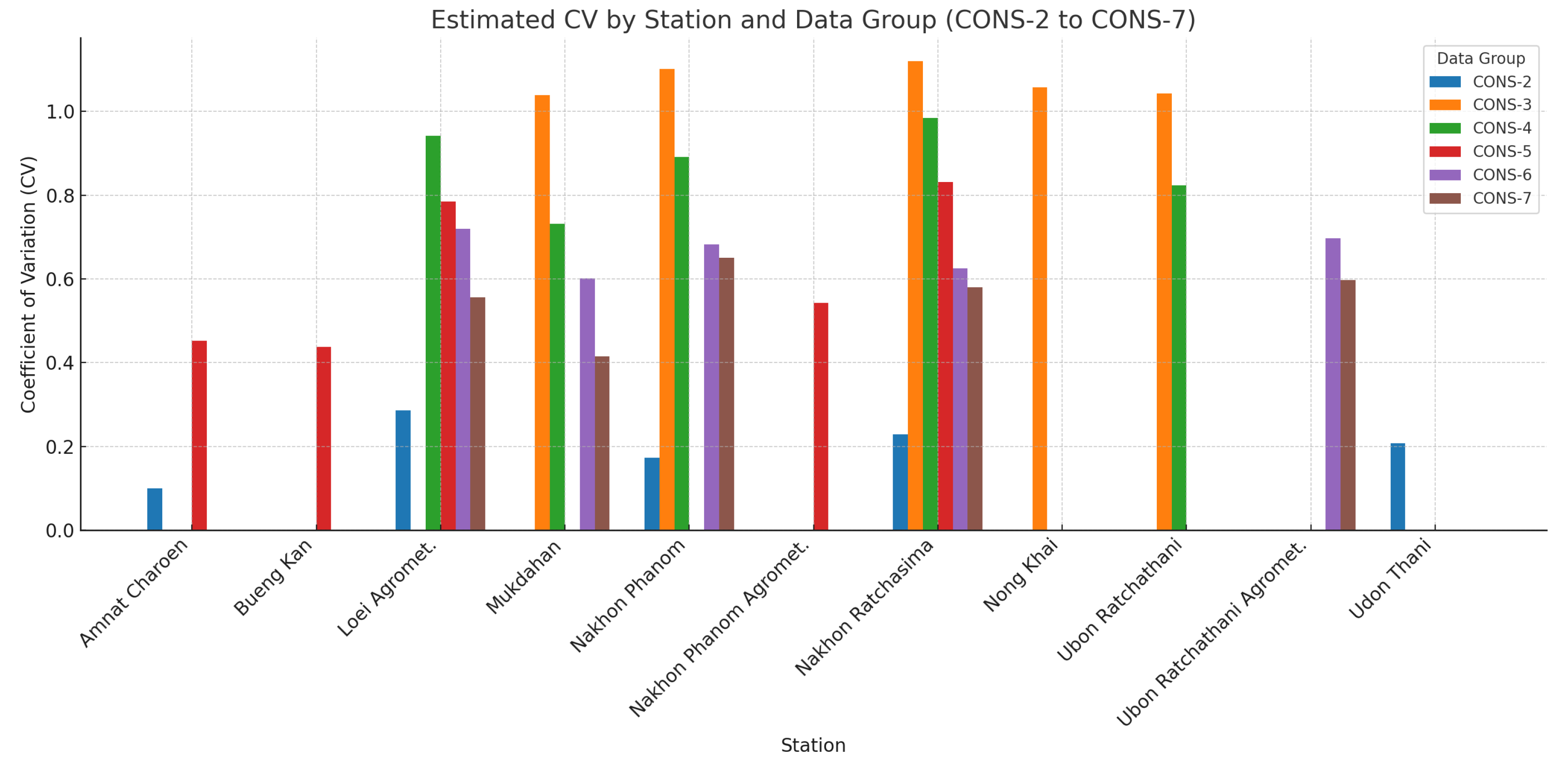
The analysis of the estimated coefficient of variation ($\widehat{\mathrm{CV}}$) for rainfall data, as presented in Table 5 and Figure 6, highlights distinct patterns of rainfall variability across different stations and data groups (CONS-2 to CONS-7). In general, lower CV values were observed in CONS-2, suggesting more stable rainfall distributions over longer periods. In contrast, CV values increased substantially in groups representing more extreme or shorter-duration rainfall events (CONS-4, CONS-6), indicating higher variability and more erratic rainfall behavior. The 95% confidence intervals across all stations remained relatively narrow, reflecting the robustness of the CV estimates. Furthermore, consistent station-level differences emerged, with some locations—such as Loei Agromet. and Nakhon Phanom—exhibiting higher rainfall variability across multiple groups. These findings underscore the importance of accounting for both temporal scale and spatial variability when modeling rainfall and assessing hydrological risks, particularly in the context of extreme events and climate adaptation planning.

7. Discussion

This study provides a comprehensive analysis of the asymptotic properties of the coefficient of variation estimator under the reparameterized Birnbaum–Saunders distribution. Our findings confirm that the method of moments-based CV estimator exhibits strong asymptotic normality properties, consistent with theoretical expectations.

The simulation results reveal clear trends across different sample sizes. In small sample settings ($n=10$ to 30), the CV estimator exhibits substantial bias and variability, making it less reliable for inference. As sample size increases to moderate levels ($n=50$ to 100), bias and variance decrease markedly, suggesting that these sample sizes are sufficient for practical applications where robust CV estimates are required. For large samples ($n=200$ to 500), the CV estimator performs exceptionally well, with minimal bias and variance approaching theoretical limits.

These findings are consistent with prior results on CV estimation in BirSau and other distributions [10,11], and extend the literature by explicitly demonstrating the behavior of the estimator under the reparameterized BirSau model. Moreover, our results complement previous interval estimation work for BirSau parameters [12] and contribute new insights specifically regarding the CV, which is of growing importance in fields such as environmental risk assessment and materials engineering.

The real-data example on rainfall modeling further illustrates the practical value of our approach. The estimated CVs across different stations and aggregation periods highlight significant spatial and temporal variability in rainfall patterns, aligning with findings from related studies on hydrological and meteorological data modeling [13,14]. The relatively narrow confidence intervals in most cases indicate the robustness of the CV estimates under the proposed method.

Taken together, these results reinforce the applicability of the reparameterized Birnbaum–Saunders distribution for modeling positively skewed environmental data and support the use of method of moments-based CV estimators in both research and applied settings.

8. Conclusions

This study rigorously investigated the asymptotic properties of the coefficient of variation estimator for the reparameterized Birnbaum–Saunders distribution using the method of moments framework. Through theoretical derivations and extensive simulation studies, we established that the estimator is asymptotically normal, with its variance converging to the derived theoretical form.

Our findings demonstrate that the estimator performs poorly in small samples but improves rapidly with increasing sample size. For moderate-to-large samples, the estimator exhibits minimal bias and variance, enabling reliable inference. These results align with and extend previous work on CV estimation under the BirSau model and provide practical guidance for its application in real-world scenarios.

The application to rainfall data underscores the practical relevance of our approach, illustrating how CV-based inference can reveal important patterns in environmental variability. The methods presented here can be readily extended to other domains where positively skewed data arise, such as reliability engineering and financial risk analysis.

9. Future Studies

Future studies may focus on enhancing the estimation of the coefficient of variation (CV) in small-sample scenarios, where bias correction techniques or Bayesian approaches could provide improved accuracy. In addition, given the strong asymptotic normality and robustness of the proposed estimator in large samples, a natural extension is the comparison of variability across multiple populations. One particularly promising direction is the development of inference procedures for the ratio of CVs from two independent Birnbaum–Saunders distributions. Furthermore, incorporating the proposed estimator into broader modeling frameworks—such as hierarchical models or spatio-temporal structures—could significantly expand the applicability of the Birnbaum–Saunders distribution in complex and high-dimensional data settings.