Modal Regression Estimation by Local Linear Approach in High-Dimensional Data Case

Abstract

This paper introduces a new nonparametric estimator for detecting the conditional mode in the functional input variable setting. The estimator integrates a local linear approach with an $L^1$-robust algorithm and treats the modal regression as the minimizer of the quantile derivative. As an asymptotic result, we derive the theoretical properties of the estimator by analyzing its convergence rate under the almost complete consistency framework. The result is stated under standard conditions, characterizing both the functional structure of the data and the local linear approximation properties of the model. Moreover, the expression of the convergence rate retains the usual form of the stochastic convergence rate in functional statistics. Simulations and real-data applications demonstrate the algorithm’s effectiveness, showing its advantage over existing methods in high-dimensional prediction tasks.

1. Introduction

In the last decade, interest in the statistical analysis of functional data has grown significantly, driven by its wide range of applications in various domains. The foundational work in this field was first established by [1,2], as pioneer works, and [3] or [4] for recent results and references. Within this field, nonparametric statistics have proven to be highly effective in modeling functional data, particularly when it comes to predicting using conditional mode and conditional quantiles. However, most of the existing nonparametric functional quantiles or mode estimators heavily depend on traditional kernel methods. In this paper, we improve the accuracy and robustness of the previous estimators using the $L^1$-local linear estimation (LLE) method.

Modal and quantile regression are popular tools in nonparametric statistics for making predictions. They present an alternative approach to traditional regression, which is based on conditional expectation. Unlike the conventional approaches, the proposed predictors often impart deeper insights, especially when the data have asymmetric or multimodal conditional densities, or when the white noise shows a heavy-tailed distribution (refer to [5] for the limitation of the conditional expectation). The latter demonstrated that the conditional mode outperforms the conditional mean. Based on this, Ref. [6] created a prediction model that uses the derivative of the conditional density for multivariate data. Theoretical progress was made by [7], who established the asymptotic distribution of modal regression estimators for independent data. Ref. [8] extended the last result to the dependent cases. Further advancements in the conditional mode prediction are comprehensively covered in [9,10]. While the cited works concern the kernel estimator of the conditional mode (CM) in finite-dimensional cases, the Nadaraya–Watson (NW) estimator was extended for functional data by [11]. They estimated this regression model by maximizing the conditional density and proved its almost complete consistency. This result has been generalized to the functional time series case by [12]. The asymptotic distribution of the NW estimator of the conditional mode was explored for the independent case in [13] and for the strongly mixing case by [14]. There were also significant theoretical advancements made by [15], who determined $L^p$-convergence rates for NW-based functional CM estimators. For an alternative functional time series, Ref. [16] established stochastic consistency for ergodic functional time series data containing missing at random. Further theoretical and practical contributions in the field of functional CM estimation can be found in [17] and the references therein.

On the other hand, quantile regression has gained increasing interest in nonparametric data analysis. It is worth noting that the quantile regression function is also one of the most well-studied models in nonparametric vector statistics. Earlier foundational works in multivariate statistics go back to [18], and were popularized by [19,20]. Once again in functional statistics, quantile regression has received considerable attention. This high level of flexibility justifies the approach, as it can be treated as a linear, semiparametric, or nonparametric model. The functional linear modeling of the conditional quantile was considered by [21,22], which provides comprehensive overviews of the latest developments. While the semiparametric estimation was developed by [23]. Concerning nonparametric estimation, quantile regression is estimated using the functional version of the NW estimator by [11]. They proved the Borel–Cantelli of the constructed estimator. Ref. [24] has stated the moment integrability of the functional NW estimator. We return to [25,26] for recent results.

The main novelty of this work is the estimation by the LLE method. This approach provides an important advantage compared to the NW estimator. In particular, it permits increasing the efficiency of the estimation by reducing bias. This statement has been observed by [27] in the multivariate case and expanded into functional statistics by [28]. From a bibliographical perspective, the LLE technique has been thoroughly explored in functional statistics by many authors. For example, Ref. [29] demonstrated $L_2$ consistency of the LLE estimator when estimating the regression operator in Hilbert spaces. Ref. [30] proposes a more general estimator allowing coverage of a wider range of functional covariates, while [31] developed an alternative estimator based on the inverse local covariance operator. Ref. [32] introduced functional LLE-fitting for nonparametric conditional models, establishing pointwise and uniform almost-complete (a.co.) consistency for the conditional density mode. The first results on the LLE-estimation of the quantile function were stated by [33]. Their estimation is obtained by inverting the cumulative distribution function (CDF) estimator introduced by [32]. An alternative was recently considered by [34] based on the M-estimation of the quantile regression.

While most current methods focus on estimating the conditional mode by optimizing a kernel-based conditional density estimator, this paper introduces a new LLE approach based on quantile regression. Unlike traditional methods, our estimator accumulates the robustness of $L_1$-regression and the performance of the LLE-estimation, which enhances its resistance to outliers and extends its accuracy as a predictor or classifier in functional statistics. Theoretically, we demonstrate the almost complete convergence of the estimator under standard conditions, with precision in the convergence rate. This new estimator’s benefits are also emphasized by comparing it to the standard one using a simulated and real data example. Our empirical analysis shows that the new estimator not only outperforms the accuracy of the previous estimators but also remains robust across a wide range of scenarios. Additionally, to demonstrate its practical value, we apply our method to predict the chemical composition of cocoa using spectrometry data. Typically, we have focused on the prediction of fat and moisture content using near-infrared spectroscopy data as functional regressors. It is well documented that near-infrared spectroscopy is a powerful, non-destructive tool for rapidly quantifying cocoa quality, allowing real-time quality control in production. Thus, combining this spectrometry processing with the proposed functional model can help chocolate producers to maintain good flavor and texture in their products, ensuring quality at every step.

The paper is organized as follows. In the next Section, we introduce the conditional mode based on the $L^1$ rule and explain its LLE estimator. Section 3 covers the principal assumptions and the main theoretical findings. In Section 4 We outline the principal features of our approach and provide a comparative analysis with existing methods. The finite-sample performance of our proposed estimator is examined in Section 5, using both simulation studies and real-world data applications. The detailed proofs of the intermediate results are presented in the Appendix A.

2. The ${\mathit{L}}^{\mathbf{1}}$ Conditional Mode and Its Local Linear Estimator

Let ${\left\{(F_i,R_i)\right\}}_{i=1}^n$ be an independent and identically distributed (i.i.d.) sample from the random pair $(F,R)$, where F is functional input variable taking values in a semi-metric space $(\mathcal{H},m)$ (m being the semi-metric) and R is the output real variable. Next, fix $\mathfrak{F}\in \mathcal{H}$ and consider a neighborhood ${\mathcal{N}}_{\mathfrak{F}}$ of $\mathfrak{F}$. We assume the existence of the regular conditional distribution function $D(·|\mathfrak{F})$ of R given $F=\mathfrak{F}$, which is strictly increasing and has a continuous density $d(·|\mathfrak{F})$ with respect to Lebesgue measure on $\mathbb{R}$. The standard conditional mode is usually defined as the maximizer of this conditional density over a compact set S:

$$MR\left(\mathfrak{F}\right)=\arg \underset{y\in S}{\max }d\left(y\right|\mathfrak{F}).$$

(1)

However, in order to introduce a more robust definition of the conditional mode, we reformulate this definition and we relate the modal regression to the quantile derivatives. Indeed, for $q\in D^{-1}\left(S\right|\mathfrak{F})=[a_{\mathfrak{F}},b_{\mathfrak{F}}]\subset (0,1)$, let $Q{R}_q\left(\mathfrak{F}\right)$ denote the conditional quantile of order q given $F=\mathfrak{F}$. Following similar ideas to [35] in the linear case, we assume $Q{R}_{·}\left(\mathfrak{F}\right)$ is continuously differentiable ($C^1$) with $D\left(Q{R}_q\left(\mathfrak{F}\right)\right|\mathfrak{F})>0$, yielding:

$$Q{R}_q^{\prime }\left(\mathfrak{F}\right)={\displaystyle \frac{\partial Q{R}_q\left(\mathfrak{F}\right)}{\partial q}}={\displaystyle \frac{1}{D\left(Q{R}_q\left(\mathfrak{F}\right)\right|\mathfrak{F})}}.$$

(2)

It follows that the conditional mode can be expressed as:

$$MR\left(\mathfrak{F}\right)=Q{R}_{q_{MR}}\left(\mathfrak{F}\right),\mathrm{where}{q}_{MR}=\arg \underset{q\in [a_{\mathfrak{F}},b_{\mathfrak{F}}]}{\min }Q{R}_q^{\prime }\left(\mathfrak{F}\right).$$

(3)

Recall that the theoretical conditional quantile $Q{R}_q\left(\mathfrak{F}\right)$ is robustly defined as M-regression with respect to the following score function

$$\underset{t}{\min }\mathbb{E}\left[L_q(R-t)\mid F=\mathfrak{F}\right],$$

(4)

where $L_q\left(y\right)=y(q-{1\mathrm{I}}_{\{y<0\}})$ is the quantile loss function. Thus, the LLE estimator of the conditional mode is strongly linked to the LLE estimator of the quantile regression. For this last point, we adopt the fast LLE approach of [30], approximating $Q{R}_q(·)$ in a neighborhood ${\mathcal{N}}_{\mathfrak{F}}$ by:

$$Q{R}_q\left(\mathfrak{Z}\right)\approx A+Bm(\mathfrak{F},\mathfrak{Z})\forall \mathfrak{Z}\in {\mathcal{N}}_{\mathfrak{F}},$$

(5)

and estimate the coefficients $(A,B)$ as solutions of

$$\underset{(A,B)\in {\mathbb{R}}^2}{\min }\sum _{i=1}^n{L}_q(R_i-A-Bm(F_i,\mathfrak{F}))\mathbf{F}\left({\displaystyle \frac{m(\mathfrak{F},F_i)}{f_n}}\right),$$

(6)

where $\mathbf{F}$ is a kernel function, $f_n$ is a bandwidth sequence. The conditional quantile estimator is then ${\widehat{QR}}_q\left(\mathfrak{F}\right)=\widehat{a}$. Consequently, the LLE estimator of the conditional mode is

$$\widehat{MR}\left(\mathfrak{F}\right)=\widehat{QR}\left({\widehat{q}}_{M}R\right|\mathfrak{F})\mathrm{where}{\widehat{q}}_{M}R=\arg \underset{q\in [a_{\mathfrak{F}},b_{\mathfrak{F}}]}{\min }{\widehat{QR}}^{\prime }\left(q\right|\mathfrak{F}),$$

(7)

with ${\widehat{QR}}^{\prime }$ being the estimator of the derivative of the conditional quantile defined by

$${\widehat{QR}}^{\prime }\left(q\right|\mathfrak{F})={\displaystyle \frac{\widehat{QR}(q+b_n|\mathfrak{F})-\widehat{QR}(q-b_n|\mathfrak{F})}{2b_n}},$$

(8)

where $b_n$ is a positive bandwidth-like sequence.

We point out that the functional NW estimator studied by [17] is a particular case of this study; it corresponds to $B=0$. Next, let us clarify that the existence and uniqueness of $MR\left(\mathfrak{F}\right)$ are guaranteed by the continuity and strict monotonicity of $D(·|\mathfrak{F})$, while $\widehat{MR}\left(\mathfrak{F}\right)$ may not be unique. In what follows, $\widehat{MR}\left(\mathfrak{F}\right)$ refers to any minimizer in (6). Furthermore, the primary contribution of this work is to establish asymptotic properties of $\widehat{MR}\left(\mathfrak{F}\right)$ when $\mathfrak{F}$ takes values in the semi-metric space ${\mathcal{F}}_{\mathcal{N}}$. To our knowledge, this is the first study to employ this estimation strategy for the conditional mode, even in multivariate settings. Note that the finite-dimensional case (${\mathcal{F}}_{\mathcal{N}}={\mathbb{R}}^p$) emerges as a special case, highlighting the generality of our approach.

3. Main Results

All along the paper, when no confusion is possible, we will denote by C or $C^{\prime }$ some strictly positive generic constants, and we set $B(\mathfrak{F},f)=\left\{{\mathfrak{F}}^{\prime }\in \mathcal{F}:m({\mathfrak{F}}^{\prime },\mathfrak{F})<f\right\}$. Now, we list some required conditions that are necessary in deriving the almost complete convergence of $\widehat{MR}\left(\mathfrak{F}\right)$ of $MR\left(\mathfrak{F}\right)$.

(B1)

For any $r>0$, ${\alpha }_{\mathfrak{F}}\left(f\right):={\alpha }_{\mathfrak{F}}(-f,f)>0$ and there exists a function ${\beta }_{\mathfrak{F}}(·)$ such that:

$$\mathrm{for}\mathrm{all}t\in (-1,1),\underset{f\to 0}{\lim }{\displaystyle \frac{{\alpha }_{\mathfrak{F}}(t{f}_n,f_n)}{{\alpha }_{\mathfrak{F}}\left(f_n\right)}}={\beta }_{\mathfrak{F}}\left(t\right)$$

(B2)

The functions $QR(·|\mathfrak{F})$ is of class $C^3\left([a_{\mathfrak{F}},b_{\mathfrak{F}}]\right)$ and $D(·|\mathfrak{F})$ satisfies the following Lipschitz condition:

$$\mathrm{for}\mathrm{all}({\mathfrak{F}}_1,{\mathfrak{F}}_2)\in N_{\mathfrak{F}},|D\left(t\right|{\mathfrak{F}}_1)-D\left(t\right|{\mathfrak{F}}_2)|\le C{d}^b({\mathfrak{F}}_1,{\mathfrak{F}}_2)\mathrm{for}\mathrm{some}b>0,$$

where $N_{\mathfrak{F}}$ denotes a neighborhood of $\mathfrak{F}$.

(B3)

The kernel $\mathbf{F}$ is a positive and differentiable function which is supported within $(-1,1)$, and such that:

$$\left(\begin{array}{cc}\mathbf{F}\left(1\right)-{\int }_{-1}^1{\mathbf{F}}^{\prime }\left(t\right){\beta }_{\mathfrak{F}}\left(t\right)dt& \mathbf{F}\left(1\right)-{\int }_{-1}^1{\left(t\mathbf{F}\left(t\right)\right)}^{\prime }{\beta }_{\mathfrak{F}}\left(t\right)dt\\ \\ \mathbf{F}\left(1\right)-{\int }_{-1}^1{\left(t\mathbf{F}\left(t\right)\right)}^{\prime }{\beta }_{\mathfrak{F}}\left(t\right)dt& \mathbf{F}\left(1\right)-{\int }_{-1}^1{\left(t^2\mathbf{F}\left(t\right)\right)}^{\prime }{\beta }_{\mathfrak{F}}\left(t\right)dt\end{array}\right)$$

is a positive definite matrix.

(B4)

The bandwidth $f_n$ satisfies:

$$\underset{n\to \infty }{\lim }{\displaystyle \frac{\log n}{n{b}_n{\alpha }_{\mathfrak{F}}\left(f_n\right)}}=0$$

The assumed conditions are not very restrictive. They allow us to analyze various aspects of our subject, such as model structure, data framework, and convergence rates. Considering the complexity of our proposed local linear algorithm and the strength of the Borel–Cantelli (BC) consistency, these assumptions offer a good compromise between generality and analytical feasibility. Specifically, each element of the subject is explored through a distinct assumption. For instance, (B1) is particularly essential in NFDA. Specifically, Condition (B1) is indispensable in NFDA, and the function ${\alpha }_{\mathfrak{F}}(.)$ can be explicitly given for several continuous processes (see [11]). While the regularity conditions are necessary to explore the functional space of the nonparametric path under study, this assumption significantly impacts the bias term in the convergence rate of $\widehat{MR}\left(\mathfrak{F}\right)$. Finally, conditions (B3)–(B4) relate to the kernel $\mathbf{F}$ and the bandwidths $f_n$ and $b_n$, which cover the technical aspects of the estimator $\widehat{MR}\left(\mathfrak{F}\right)$. These conditions are less restrictive than the usual technical requirements in conditional mode estimation. Unlike the conditional density approach, which relies on two kernels, our method requires only one. It is important to recall that these conditions are necessary to determine the convergence rate of the kernel estimator under the Borel–Cantelli mode. Typically, a weaker form of consistency—distinct from BC consistency—can be established for the estimator under more restrictive assumptions. The latter is obtained by evaluating the expectation and variance of the estimator. Although this probability consistency is weaker than Borel–Cantelli consistency, it remains sufficient to justify the estimator’s practical applicability. Nevertheless, because this paper aims to demonstrate both the theoretical generality of the model and its practical viability, we have chosen to emphasize the stronger consistency result, which implies the weaker.

The following theorem establishes the almost-complete convergence (cf. [2] for details), (a.co.), of $\widehat{MR}\left(\mathfrak{F}\right)$. This kind of convergence implies both almost sure convergence and convergence in probability.

Theorem 1.

Under assumptions (B1)–(B4) and if ${\displaystyle \underset{q\in (0,1)}{\inf }\frac{{\partial }^{3}Q{R}_q\left(\mathfrak{F}\right)}{\partial q}>0}$ we have:

$$\widehat{MR}\left(\mathfrak{F}\right)-MR\left(\mathfrak{F}\right)=O\left(f_n^{b/2}\right)+O\left(b_n^{1/2}\right)+O\left({\left({\displaystyle \frac{\log n}{n{b}_n^2{\alpha }_{\mathfrak{F}}\left(f_n\right)}}\right)}^{{\displaystyle \frac{1}{4}}}\right)a.co.$$

Proof of Theorem 1.

The proof is based on some standard analytical arguments. Indeed, we write

$$\widehat{MR}\left(\mathfrak{F}\right)-MR\left(\mathfrak{F}\right)={\widehat{QR}}_{\widehat{q_{MR}}}\left(\mathfrak{F}\right)-{QR}_{\widehat{q_{MR}}}\left(\mathfrak{F}\right)+{QR}_{\widehat{q_{MR}}}\left(\mathfrak{F}\right)-{QR}_{q_{MR}}\left(\mathfrak{F}\right)$$

Trivially,

$$\widehat{MR}\left(\mathfrak{F}\right)-MR\left(\mathfrak{F}\right)\le \underset{q\in [a_{\mathfrak{F}},b_{\mathfrak{F}}]}{\sup }|\widehat{QR}\left(q\right|\mathfrak{F})-t\left(q\right|\mathfrak{F})|+{QR}_{\widehat{q_{MR}}}\left(\mathfrak{F}\right)-{QR}_{q_{MR}}\left(\mathfrak{F}\right)$$

By Taylor expansion,

$${QR}_{\widehat{q_{MR}}}\left(\mathfrak{F}\right)-{QR}_{q_{MR}}\left(\mathfrak{F}\right)=(\widehat{q_{MR}}-q_{MR})Q{R}_{q_{MR}^{*}}^{\prime }\left(\mathfrak{F}\right),q_{MR}^{*}\mathrm{being}\mathrm{in}(\widehat{q_{MR}},q_{MR}).$$

(9)

Since $q_{MR}$ is minimizer of $Q{R}_{·}^{\prime }\left(\mathfrak{F}\right)$,

$${Q{R}^{\prime }}_{\widehat{q_{MR}}}\left(\mathfrak{F}\right)-{Q{R}^{\prime }}_{q_{MR}}\left(\mathfrak{F}\right)={(\widehat{q_{MR}}-q_{MR})}^{2}Q{R}_{q_{MR}^{**}}^{\prime \prime \prime }\left(\mathfrak{F}\right),\mathrm{where}{q}_{MR}^{**}\in (\widehat{q_{MR}},q_{MR}).$$

(10)

In addition,

$$\begin{array}{cc}Q{R}_{\widehat{q_{MR}}}^{\prime }\left(\mathfrak{F}\right)-Q{R}_{q_{MR}}^{\prime }\left(\mathfrak{F}\right)& =Q{R}_{\widehat{q_{MR}}}^{\prime }\left(\mathfrak{F}\right)-{\widehat{Q{R}^{\prime }}}_{\widehat{q_{MR}}}\left(\mathfrak{F}\right)+{\widehat{Q{R}^{\prime }}}_{\widehat{q_{MR}}}\left(\mathfrak{F}\right)-{QR}_{q_{MR}}\left(\mathfrak{F}\right)\hfill \\ & \le |Q{R}_{\widehat{q_{MR}}}^{\prime }\left(\mathfrak{F}\right)-{\widehat{Q{R}^{\prime }}}_{\widehat{q_{MR}}}\left(\mathfrak{F}\right)|+|\underset{q}{\min }{\widehat{Q{R}^{\prime }}}_q\left(\mathfrak{F}\right)-\underset{q}{\min }Q{R}_q^{\prime }\left(\mathfrak{F}\right)|\hfill \\ & \le 2{\sup }_{q\in [a_{\mathfrak{F}},b_{\mathfrak{F}}]}|{\widehat{Q{R}^{\prime }}}_q\left(\mathfrak{F}\right)-Q{R}_q^{\prime }\left(\mathfrak{F}\right)|\hfill \end{array}$$

(11)

Thus,

$$|\widehat{MR}\left(\mathfrak{F}\right)-MR\left(\mathfrak{F}\right)|\le C\left(\underset{q\in [a_{\mathfrak{F}},b_{\mathfrak{F}}]}{\sup }|{\widehat{QR}}_q\left(\mathfrak{F}\right)-Q{R}_q\left(\mathfrak{F}\right)|+\sqrt{\underset{q\in [a_{\mathfrak{F}},b_{\mathfrak{F}}]}{\sup }|{\widehat{Q{R}^{\prime }}}_q\left(\mathfrak{F}\right)-Q{R}_q^{\prime }\left(\mathfrak{F}\right)|}\right).$$

Now, for a large enough n

$$\begin{array}{cc}{\widehat{Q{R}^{\prime }}}_q\left(\mathfrak{F}\right)-Q{R}_q^{\prime }\left(\mathfrak{F}\right)& {\displaystyle =\frac{{\widehat{QR}}_{q+b_n}\left(\mathfrak{F}\right)-Q{R}_{q+b_n}\left(\mathfrak{F}\right)+Q{R}_{q-b_n}\left(\mathfrak{F}\right)-{\widehat{QR}}_{q-b_n}\left(\mathfrak{F}\right)}{2b_n}}\hfill \\ & {\displaystyle +\frac{Q{R}_{q+b_n}\left(\mathfrak{F}\right)-Q{R}_q\left(\mathfrak{F}\right)+Q{R}_q\left(\mathfrak{F}\right)-Q{R}_{q-b_n}\left(\mathfrak{F}\right)-2b_{n}Q{R}_q^{\prime }\left(\mathfrak{F}\right)}{2b_n}}\hfill \\ \\ & {\displaystyle \le C{b}_n^{-1}\underset{q\in (a_{\mathfrak{F}}-b_n,b_{\mathfrak{F}}+b_n)}{\sup }|{\widehat{QR}}_q\left(\mathfrak{F}\right)-Q{R}_q\left(\mathfrak{F}\right)|+O\left(b_n\right)}\hfill \end{array}$$

Thus, it suffices to evaluate, for a large enough n

$$\underset{q\in [0,1]}{\sup }|{\widehat{QR}}_q\left(\mathfrak{F}\right)-Q{R}_q\left(\mathfrak{F}\right)|.$$

Thus, Theorem 1 is a consequence of the following proposition. □

Proposition 1.

Under assumptions of Theorem 1, we have

$$\underset{q\in (0,1)}{\sup }|{\widehat{QR}}_q\left(\mathfrak{F}\right)-Q{R}_q\left(\mathfrak{F}\right)|=O\left(f_n^b\right)+O_{a.co.}\left({\left({\displaystyle \frac{\log n}{n{\alpha }_{\mathfrak{F}}\left(f_n\right)}}\right)}^{{\displaystyle \frac{1}{2}}}\right)$$

The proof of this proposition is based on the Bahadur representation of the conditional quantile. The latter is a consequence of the following lemmas.

Lemma 1.

Let ${\Pi }_n$ be a sequence of decreasing real random functions and ${\mathrm{{\rm Y}}}_n$ be a random real sequence such that

$${\displaystyle {\mathrm{{\rm Y}}}_n=o_{a.co.}\left(1\right)and\underset{\left|\nu \right|\le M}{\sup }|{\Pi }_n\left(\nu \right)+\lambda \nu -{\mathrm{{\rm Y}}}_n|=o_{a.co.}\left(1\right)forcertainconstants\lambda ,M>0.}$$

Then, for any real sequence ${\nu }_n$ such that ${\Pi }_n\left({\nu }_n\right)=o_{a.co.}\left(1\right)$, we have:

$$\sum _{n=1}^{\infty }\mathrm{I}\mathrm{P}\left\{|{\nu }_n|\ge M\right\}<\infty .$$

4. On the Potential Impact of the Contribution

• Comparison with existing approaches
  In an earlier contribution [36], we have investigated robust mode estimation under a functional single-index structure, employing the local constant method. Alternatively, in this study, we examine local linear estimation for the same model under a general functional framework. Firstly, observe that the topic of the present contribution can be viewed as a generalization of [36], in the sense that the local constant constitutes a particular case of the local linear approach, and the functional single index structure is a special case of the general functional structure. Moreover, it is well documented (see, for instance, [27]) that the local linear method has many advantages over the Nadaraya–Watson (the local constant method). Particularly, the local linear estimation is usually used to reduce the bias and the boundary effect of the Nadaraya–Watson method. So, the use of the local linear method instead of the standard kernel method substantially improves the prediction accuracy. On the other hand, it is widely recognized that the single-index model reduces analytical complexity by projecting functional covariates onto a univariate index. Thus, it transforms the functional data analysis problem into a one-dimensional real data issue. This oversimplification is unusual in practice, as it ignores potentially influential higher-dimensional interactions. Our generalized framework of this contribution circumvents this limitation. From a practical point of view, the kernel estimator assumes that the nonparametric model is flat within the neighborhood of the location point, which leads to suboptimal prediction. In contrast, the local linear method assumes that the model has a linear approximation in the neighborhood of the location point, which is more realistic and improves the prediction results.
• On the bias reduction
  As mentioned in the previous comment, the behavior of the bias term is one of the main reasons for adopting the local linear method. Although the asymptotic behavior of the bias term is usually linked to the smoothness assumptions of the nonparametric model, this term can be significantly improved in the local linear approach. This beneficial characteristic is related to the weighting functions in the local linear estimator (see [27] in the non-functional case). A similar statement can be deduced in the functional case. Specifically, under standard conditions, the local linear approach offers a better bias term compared to the Nadaraya–Watson [36]. Indeed, this improvement is also due to the specific weighting functions implemented in ${\widehat{QR}}_q\left(\mathfrak{F}\right)$. It is clear that the leading term of the Bahadur representation of ${\widehat{QR}}_q\left(\mathfrak{F}\right)$ such that

  $$\mathrm{I}\mathrm{E}\left[{\mathbf{D}}_i(A_3{\mathbf{F}}_i-A_2{f}_n^{-1}{\mathbf{D}}_i{\mathbf{F}}_i)\right]=0$$

  where

  $${\mathbf{F}}_i=\mathbf{F}\left(f_n^{-1}m(\mathfrak{F},F_i)\right),\mathrm{and}{\mathbf{D}}_i=m(F_i,\mathfrak{F})$$

  and

  $$A_j={\alpha }_{\mathfrak{F}}^{-1}\left(f_n\right)f_n^{1-j}\mathrm{I}\mathrm{E}\left[{\mathbf{D}}_i^{j-1}{\mathbf{F}}_i\right];j=2,3.$$
  Using the same analytical arguments as in [37], we prove that the first part of the bias term can be reduced to $o\left(f_n^{b/2}\right)$. In conclusion, although the local linear and the Nadaraya–Watson (NW) estimators share similar asymptotic properties, the local linearity of the model and the weighting functions of the LLE method allow us to improve the bias term in certain situations.
• On the applicability of the estimator
  Of course, the simple use of the estimator greatly depends on choosing its parameters easily. Since the estimator is derived from quantile regression, there are multiple cross-validation methods available for selecting the parameters, particularly the bandwidth parameters associated with the functional component. First, for a given subset $H_n$ of real positive numbers, we consider the cross-validation criterion used by [38].

  $$\arg \underset{f_n\in H_n}{\min }{\displaystyle \frac{1}{n}}\sum _{i=1}^n{\left(Q_p^L\left(F_i\right)-{\widehat{Q}}_p^{-i}\left(F_i\right)\right)}^2,$$

  where $Q_p^L\left(X_{\mathbf{i}}\right)$ denotes a local empirical quantile and ${\widehat{Q}}_p^{-i}$ is the conditional quantile estimator at $F_i$ after excluding this observation from the sample. Secondly, we apply the cross-validation approach that was utilized by [39]

  $$\arg \underset{f_n\in H_n}{\min }{\displaystyle \frac{1}{n}}\sum _{i=1}^n{L}_p\left(R_i-{\widehat{Q}}_p^{-i}\left(F_i\right)\right).$$
  Additionally, various other methods can be utilized, such as the least squares cross-validation technique suggested by [6]:

  $$\arg \underset{f_n\in H_n}{\min }{\displaystyle \frac{1}{n}}\sum _{i=1}^n{\left[R_i-\widehat{MR}\left(F_i\right)\right]}^2.$$
  Of course, the diversity of selection methods makes the estimator easier to implement in practice.

5. Computational Part

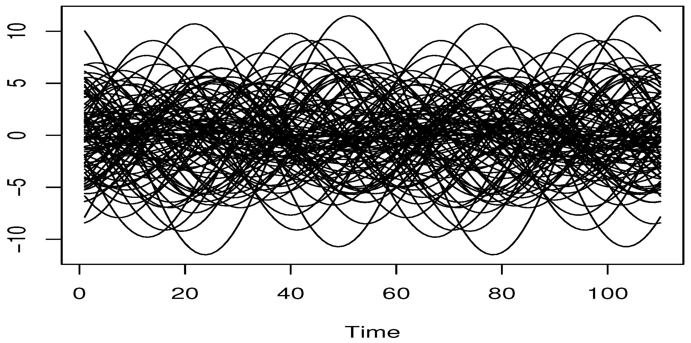
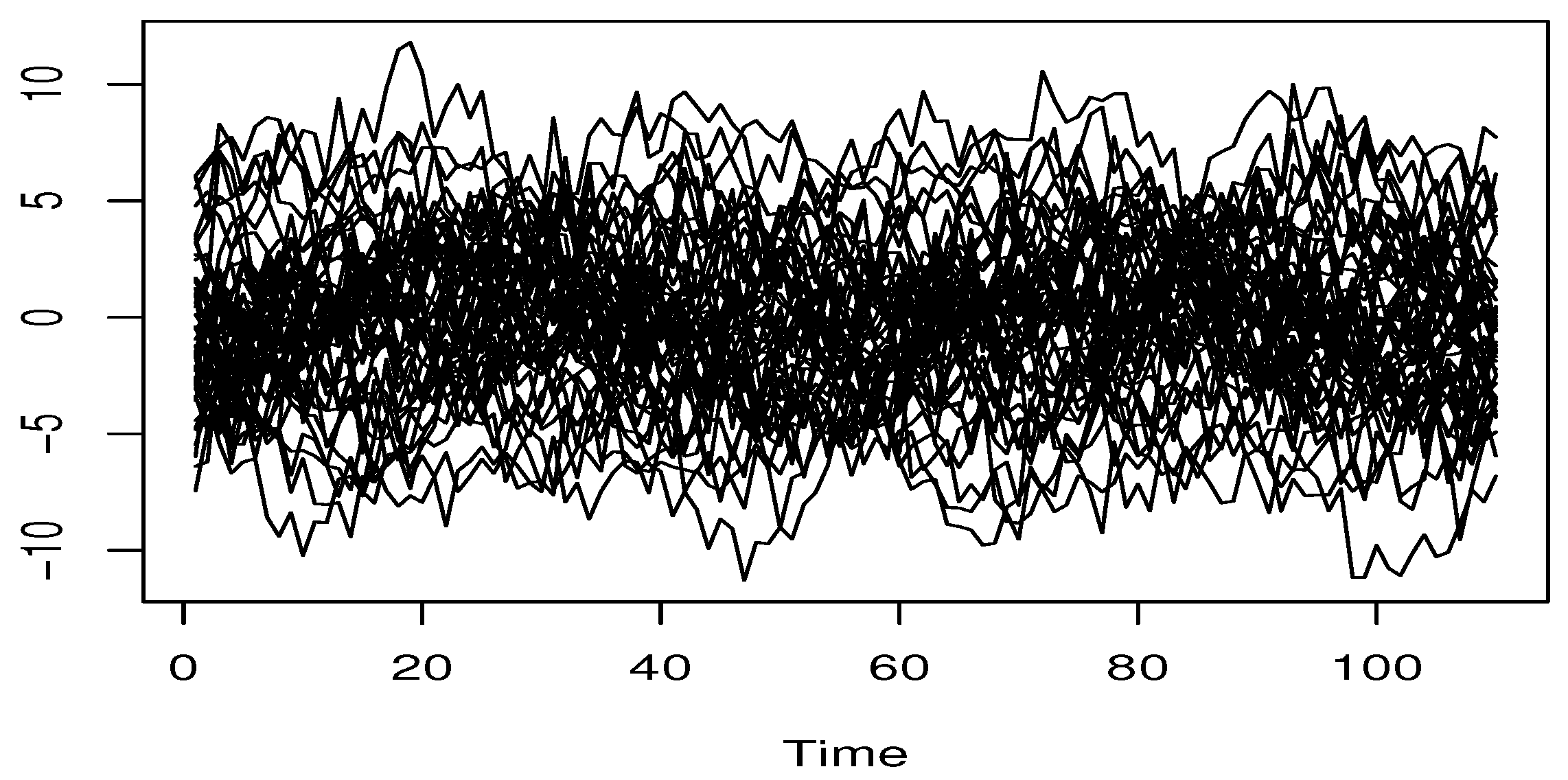
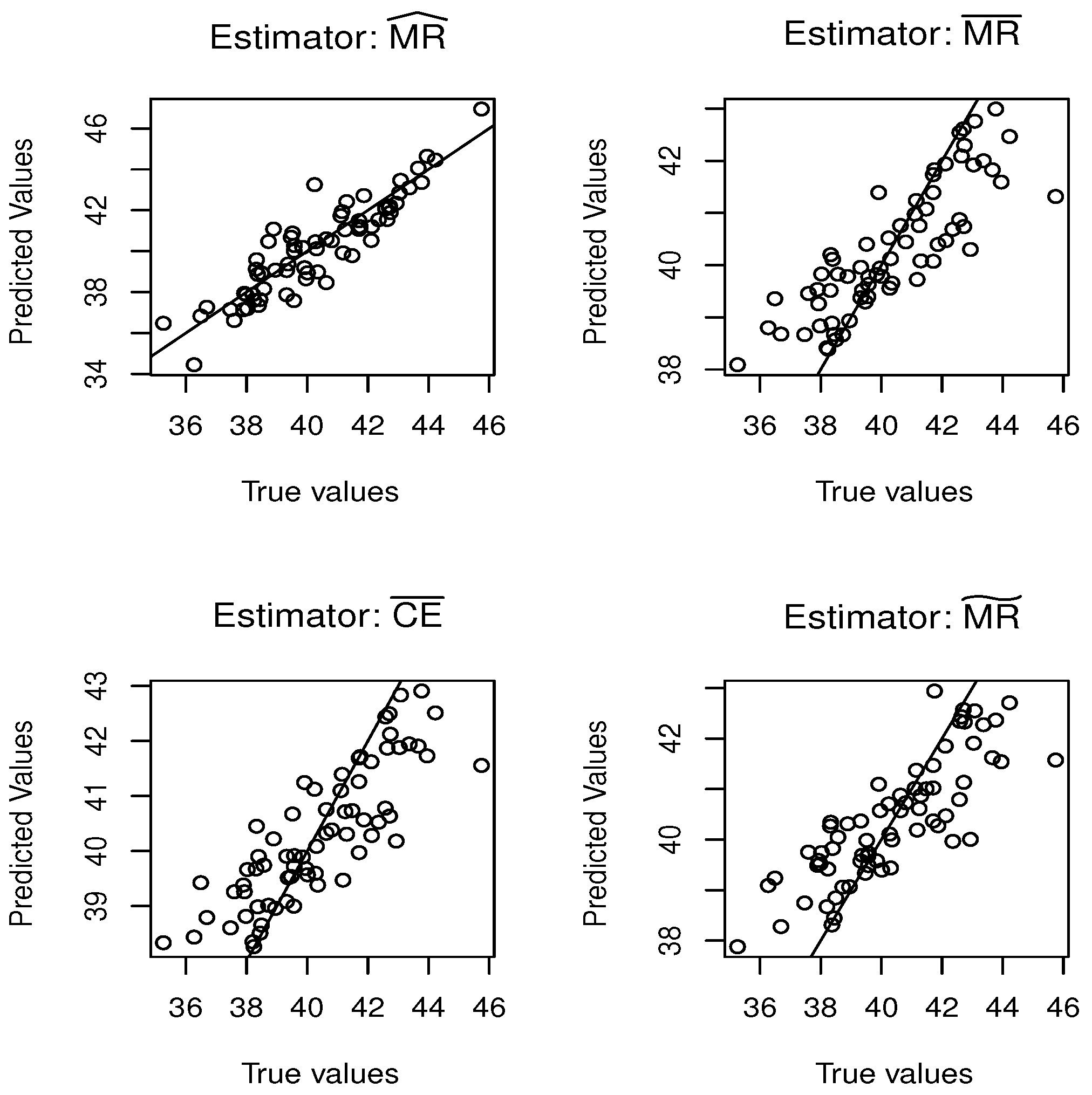
5.1. Simulation Study

In this section, we demonstrate the practical effectiveness of our theoretical development through some simulation experiments. Our principal goal is to show the easy insertion of the estimator in practice and to emphasize clear benefits of the proposed estimator over its competitors, such as the kernel conditional mode and the conditional density-based LLE-mode. In order to cover many practical situations, we generate data from different scenarios. Indeed, we consider two different nonparametric functional models that are:

$$\begin{array}{ccc}\hfill \mathit{heteroscedastic}(\mathit{Het}.)\mathit{Model}:R_i& =& 4{\int }_0^1\exp ({\displaystyle \frac{1}{3+F_i^3\left(t\right)}})dt+\cos \left(3+F_i^3\left(t\right)\right){ϵ}_i,\hfill \\ \hfill \mathit{homoscedastic}(\mathit{Hom}.)\mathit{Model}:R_i& =& 5{\int }_0^1\log \left({\displaystyle \frac{2+F_i^2\left(t\right)}{3+F_i^3\left(t\right)}}\right)dt+{ϵ}_i,\hfill \end{array}$$

where ${ϵ}_i$ and $F_i$ are independent. The functional input variable is also generated in two ways: smoothly and roughly. The smooth way is generated according to the following formula:

$$\mathit{Smooth}\mathit{curves}{F}_i\left(t\right)=a_i\cos \left(4(b_i-t\pi )\right)+b_i$$

while the rough way is drawn from the following equation:

$$\mathit{rough}\mathit{curves}{F}_i\left(t\right)=a_i\cos \left(4(b_i-t\pi )\right)+b_i+{\eta }_{i,t}$$

For both cases, $b_i$ is distributed in $N(0,0.7)$) and $a_i$ is generated according to a $N(3,4)$ distribution, while the random variables ${\eta }_{i,t}$) are drawn from $N(0,2)$. All the input curves $F_i$’s are discretized on the same grid represented by 100 equispaced measurements taken in the interval $(0,1)$. The resulting functional variables are shown in Figure 1 and Figure 2.

Obviously, choosing various curve forms is essential for evaluating how the data’s functional structure affects the accuracy of estimates. Typically, the spline metric is used for modeling smooth curves, while the PCA metric is used for rough curves.

This strategy of data sampling is intentional. It allows us to test the robustness of different models and assess how the data functionality affects the estimation accuracy. We also evaluate the nonparametric model using three distributions: Normal, Weibull, and Laplace. These were chosen because they remain consistent under translation and exhibit different levels of heavy-tailed behavior, which helps us to measure how well the estimators handle outliers. In mathematical terms, the two competitors’ modal regression estimators are defined by:

$$\mathrm{The}\mathrm{NW}\mathrm{estimator}:\widetilde{MR}\left(\mathfrak{F}\right)=\arg \underset{y}{\max }{\displaystyle \frac{{\displaystyle \sum _{i=1}^n\mathbf{F}\left(f_n^{-1}m(\mathfrak{F},F_i)\right)\mathbf{F}\left(b_n^{-1}(y-R_i)\right)}}{{\displaystyle \sum _{i=1}^n{b}_n\mathbf{F}\left(f_n^{-1}m(\mathfrak{F},F_i)\right)}}},$$

(12)

$$\mathrm{and}\mathrm{the}\mathrm{LLEestimator}:\overline{MR}\left(\mathfrak{F}\right)=\arg \underset{y}{\max }{\displaystyle \frac{{\displaystyle \sum _{i,j=1}^n{\mathbf{W}}_{ij}\mathbf{F}\left(b_n^{-1}(y-R_j)\right)}}{{\displaystyle \sum _{i,j=1}^n{b}_n{\mathbf{W}}_{ij}}}},$$

(13)

where $W_{ij}\left(x\right)=m(F_i,\mathfrak{F},)\left(m(F_i,\mathfrak{F},)-m(F_j,\mathfrak{F},)\right)\mathbf{F}\left(f_n^{-1}m(\mathfrak{F},F_i)\mathbf{F}\right(f_n^{-1}m(\mathfrak{F},F_j)$.

Of course, the behavior of the three estimators, $\widehat{MR}$, $\widetilde{MR}$, and $\overline{MR}$, as well as their straightforward insertion, is influenced by the choice of parameters, metric m, kernel $\mathbf{F}$, and smoothing parameters $(f_n,b_n)$. Evidently, the selection of the metric m is intrinsically linked to the smoothness of the functional curves. Smoother curves are better analyzed by the B-spline metric, which accommodates their regularity, while rougher curves require the PCA-metric to handle their more irregular structure. We refer to [2] for more details on the definitions of these metrics. The choice of kernel is motivated by technical considerations. In order to incorporate the assumption (B3), we have simulated using the quadratic kernel in $(-1,1)$. For the smoothing parameters $(f_n,b_n)$, we have used the cross-validation rule based on the mean square error defined by

$$MSE\left(\ddot{MR}\right)={\displaystyle \frac{1}{n}}\sum _{i=1}^n{\left(R_i-\ddot{MR}\left(F_i\right)\right)}^2,$$

(14)

where $\ddot{MR}$ represents either $\widehat{MR}$, $\overline{MR}$, or $\widetilde{MR}$. It follows that

$$(f^{opt},b^{opt})=\arg \underset{f_n\in {\mathbf{H}}_n,b_n\in {\mathbf{B}}_n}{\min }MSE\left(\ddot{MR}\right)$$

${\mathbf{H}}_n$ (respectively, ${\mathbf{B}}_n$ ) is the set of positive real numbers, $f_n$, such that the ball centered at $\mathfrak{F}$ with radius $f_n$ (respectively, the interval $[y-b_n,y+b_n]$) contains exactly k neighbors of (respectively, y). Typically, the number k is selected from the subset $\{5,10,20,\dots ,0.5\ast n\}$. For our goal, we generate $n=200$ observations of $(F_i,R_i)$, and we examine the robustness and the accuracy of different estimators using the MSE defined in (14). The obtained results are reported in the following table.

The performance of these estimators is strongly influenced by various components of the study, particularly the nature of the functional data and the nonparametric approach. Nevertheless, combining $L^1$-techniques with the LLE-smoothing method proves highly advantageous in terms of robustness and accuracy. As evidenced by the MSE results in

Table 1. $MSE$ for different estimators in different scenarios.

Cond. Dist.	Model	CURVES	$\widehat{\mathbf{MR}}$	$\overline{\mathbf{MR}}$	$\widetilde{\mathbf{MR}}$
Normal	Hom.model	Smooth	0.0258	0.0897	0.1672
		Rough	0.1067	0.4676	0.5679
Normal	Het.model	Smooth	0.2672	0.7426	1.0578
		Rough	0.3617	1.2725	1.8811
Laplace	Hom. model	Smooth	0.4257	0.6150	0.6317
		Rough	0.9804	1.0922	1.1788
Laplace	Het. model	Smooth	0.8967	1.6824	1.7088
		Rough	0.9176	2.4521	2.6588
Weibull	Hom. model	Smooth	0.5179	1.5005	1.5446
		Rough	0.8399	2.4873	2.7098
Weibull	Het. model	Smooth	0.7840	1.6253	1.4102
		Rough	0.9705	3.3567	4.3456

, the variability in $\widehat{MR}$ is lower than that of the other estimators. This lower variability demonstrates that the $L^1$-LLE estimator for the conditional mode offers greater robustness and improved accuracy.

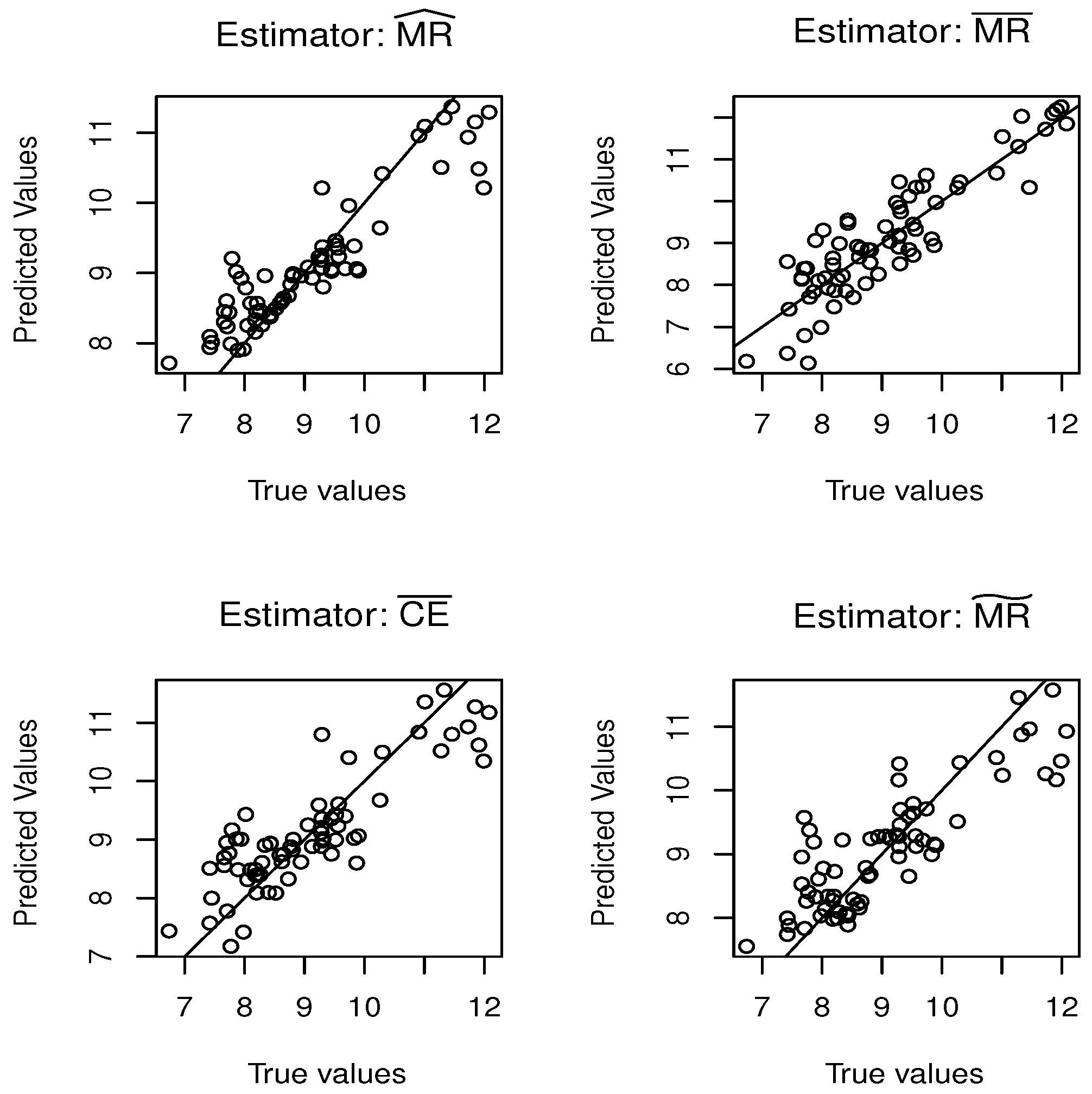
5.2. Real Data Application

Spectrometry data analysis is a powerful tool for generating high-frequency functional data. In this study, we focus on food quality as a critical real-world issue. Clearly, ensuring high-quality food is a top priority for both consumers and producers. Traditionally, quality control relies on chemical testing as an effective but destructive, time-consuming, and expensive approach. Instead, we provide a smart solution that combines spectrometry techniques with advanced statistical tools. It permits us to create an efficient, cost-effective, and non-invasive approach to ensure food quality. Specifically, we demonstrate how our new predictor can accurately predict fat and moisture contents in chocolate. Therefore, we evaluate our approach against leading alternatives, including the NW estimator, LLE-conditional expectation, and density-based LLE-mode. This computational study allows us to demonstrate the superiority and practical advantages of $\widehat{MR}$ in robustness as well as in accuracy. We compare these three approaches by testing their predictive performance using the near-infrared spectroscopy curve as functional input F, with the fat (or moisture) quantity as response variable R. The near-infrared data set available on the website (https://data.mendeley.com/datasets/7734j4fd98/1, (accessed on 8 May 2025)). This issue has been considered by many authors using different algorithms (see [40] for a list of references). Formally, in this real data example, we assume that the spectrum curve gives the absorbance of light across wavelengths ranging from 1000 to 2500 nm. These curves are visualized in Figure 3.

These curves represent the absorbance spectrum (NIR) in the wavelength range from 1000 to 2500 nm for a total of 72 bulk intact cocoa bean samples. Each bulk amounted to 50 g of intact beans. Recall that the choice of the response variable R is motivated by the fact that the fat or moisture quantities are determinants of cocoa quality. The quality of cocoa beans is the cornerstone of exceptional chocolate production, profoundly influencing the sensory, nutritional, and commercial value of the final product. Thus, precise determination of cocoa contents is essential for compliance with chocolate quality standards, economic valuation, and research in agriculture and nutrition. Consequently, optimizing fat and moisture percentage is primordial to delivering high-quality chocolate products that meet both consumer and industry demands. Now, to put our predictors into action, we need to carefully select the principal parameters that drive our estimator’s performance. This step is crucial to ensuring the potential feasibility of the four predictors $\widehat{MR}$, $\widetilde{MR}$, $\overline{MR}$, and

$$\overline{CE}={\displaystyle \frac{{\displaystyle \sum _{i,j=1}^n{\mathbf{W}}_{ij}{R}_j}}{{\displaystyle \sum _{i,j=1}^n{b}_n{\mathbf{W}}_{ij}}}},$$

Based on our earlier discussion, the kernel selection is a direct consequence of assumption (B3), ensuring theoretical consistency. Meanwhile, the metric m plays a crucial role in the quantification of the smoothness of the functional curves $F_i$, allowing us to better analyze their behavior. Clearly, the curve’s shape in Figure 3 shows that the metric of $L_2$ between the first derivatives of the curves (the curves being regular) is more suitable for this data. Once again, the smoothing parameters $(f_n,b_n)$ according the same strategy as in (14). This latest approach has proven highly effective in our predictive modeling, highlighting the importance of leave-one-out cross-validation data-driven algorithms in functional data analysis. Figure 4 and Figure 5 summarize our statistical predictions for fat and moisture for the 70 observations, comparing each approach’s performance by plotting predicted values against the true values.

We use (MSE) error to assess model performance for the predictiom results. It is defined by

$$MSE\left(\ddot{\theta }\right)={\displaystyle \frac{1}{70}}\sum _{i=1}^{70}{\left(R_i-\ddot{MR}\left(F_i\right)\right)}^2,$$

where $\ddot{\theta }$ can represent either $\widehat{MR}$, $\overline{MR}$, $\widetilde{MR}$ or $\overline{CE}$. Clearly, the predictor $\widehat{MR}$ outperforms the other predictors in precision. The latter predicts (fat, moisture) with MSE equal, respectively, to $(0.97,1.06)$. It is the best one compared to the results obtained by the predictors $\overline{MR}$, $\widetilde{MR}$, and $\overline{CE}$. Typically, we record for both components (fat, moisture) $(1.70,2,89)$ for $\overline{MR}$, $(4.89,7.48)$ for $\widetilde{MR}$ and $(3.45,6.22)$ for $\overline{CE}$.

References

1. Ramsay, J.O.; Silverman, B.W. Functional Data Analysis, 2nd ed.; Springer: New York, NY, USA, 2005. [Google Scholar]
2. Ferraty, F.; Vieu, P. Nonparametric Functional Data Analysis. Theory and Practice; Springer Series in Statistics; Springer: New York, NY, USA, 2006. [Google Scholar]
3. Xu, Y. Functional Data Analysis. In Springer Handbook of Engineering Statistics; Springer: London, UK, 2023; pp. 67–85. [Google Scholar]
4. Ahmed, M.S.; Frévent, C.; Génin, M. Spatial Scan Statistics for Functional Data. In Handbook of Scan Statistics; Springer: New York, NY, USA, 2024; pp. 629–645. [Google Scholar]
5. Collomb, G.; Härdle, W.; Hassani, S. A note on prediction via estimation of the conditional mode function. J. Stat. Plan. Inference 1986, 15, 227–236. [Google Scholar] [CrossRef]
6. Quintela-Del-Rio, A.; Vieu, P. A nonparametric conditional mode estimate. J. Nonparametr. Stat. 1997, 8, 253–266. [Google Scholar] [CrossRef]
7. Ioannides, D.; Matzner-Løber, E. A note on asymptotic normality of convergent estimates of the conditional mode with errors-in-variables. J. Nonparametr. Stat. 2004, 16, 515–524. [Google Scholar] [CrossRef]
8. Louani, D.; Ould-Saïd, E.L.I.A.S. Asymptotic normality of kernel estimators of the conditional mode under strong mixing hypothesis. J. Nonparametr. Stat. 1999, 11, 413–442. [Google Scholar] [CrossRef]
9. Bouzebda, S.; Khardani, S.; Slaoui, Y. Asymptotic normality of the regression mode in the nonparametric random design model for censored data. Commun. Stat. Theory Methods 2023, 52, 7069–7093. [Google Scholar] [CrossRef]
10. Bouzebda, S.; Didi, S. Some results about kernel estimators for function derivatives based on stationary and ergodic continuous time processes with applications. Communications in Statistics. Theory Methods 2022, 51, 3886–3933. [Google Scholar] [CrossRef]
11. Ferraty, F.; Laksaci, A.; Vieu, P. Estimating some characteristics of the conditional distribution in nonparametric functional models. Stat. Inference Stoch. Process. 2006, 9, 47–76. [Google Scholar] [CrossRef]
12. Bouzebda, S.; Chaouch, M.; Laïb, N. Limiting law results for a class of conditional mode estimates for functional stationary ergodic data. Math. Methods Stat. 2016, 25, 1066–5307. [Google Scholar] [CrossRef]
13. Ezzahrioui, M.H.; Ould-Saïd, E. Asymptotic normality of a nonparametric estimator of the conditional mode function for functional data. J. Nonparametr. Stat. 2008, 20, 3–18. [Google Scholar] [CrossRef]
14. Ezzahrioui, M.H.; Saïd, E.O. Some asymptotic results of a non-parametric conditional mode estimator for functional time-series data. Stat. Neerl. 2010, 64, 171–201. [Google Scholar] [CrossRef]
15. Dabo-Niang, S.; Kaid, Z.; Laksaci, A. Asymptotic properties of the kernel estimate of spatial conditional mode when the regressor is functional. AStA Adv. Stat. Anal. 2015, 99, 131–160. [Google Scholar] [CrossRef]
16. Bouanani, O.; Laksaci, A.; Rachdi, M.; Rahmani, S. Asymptotic normality of some conditional nonparametric functional parameters in high-dimensional statistics. Behaviormetrika 2019, 46, 199–233. [Google Scholar] [CrossRef]
17. Azzi, A.; Belguerna, A.; Laksaci, A.; Rachdi, M. The scalar-on-function modal regression for functional time series data. J. Nonparametr. Stat. 2024, 36, 503–526. [Google Scholar] [CrossRef]
18. Stone, C.J. Consistent nonparametric regression. Ann. Stat. 1977, 5, 595–620. [Google Scholar] [CrossRef]
19. Koenker, R.; Zhao, Q. Conditional quantile estimation and inference for ARCH models. Econom. Theory 1996, 12, 793–813. [Google Scholar] [CrossRef]
20. Hallin, M.; Lu, Z.; Yu, K. Local linear spatial quantile regression. Bernoulli 2009, 15, 659–686. [Google Scholar] [CrossRef]
21. Cardot, H.; Crambes, C.; Sarda, P. Quantile regression when the covariates are functions. J. Nonparametr. Stat. 2005, 17, 841–856. [Google Scholar] [CrossRef]
22. Wang, H.; Ma, Y. Optimal subsampling for quantile regression in big data. Biometrika 2021, 108, 99–112. [Google Scholar] [CrossRef]
23. Jiang, Z.; Huang, Z. Single-index partially functional linear quantile regression. Commun. Stat.-Theory Methods 2024, 53, 1838–1850. [Google Scholar] [CrossRef]
24. Dabo-Niang, S.; Kaid, Z.; Laksaci, A. Spatial conditional quantile regression: Weak consistency of a kernel estimate. Rev. Roum. Math. Pures Appl. 2012, 57, 311–339. [Google Scholar]
25. Chowdhury, J.; Chaudhuri, P. Nonparametric depth and quantile regression for functional data. Bernoulli 2019, 25, 395–423. [Google Scholar] [CrossRef]
26. Mutis, M.; Beyaztas, U.; Karaman, F.; Lin Shang, H. On function-on-function linear quantile regression. J. Appl. Stat. 2025, 52, 814–840. [Google Scholar] [CrossRef] [PubMed]
27. Fan, J. Local Polynomial Modelling and Its Applications: Monographs on Statistics and Applied Probability 66; Routledge: Abingdon-on-Thames, UK, 2018. [Google Scholar]
28. Rachdi, M.; Laksaci, A.; Demongeot, J.; Abdali, A.; Madani, F. Theoretical and practical aspects of the quadratic error in the local linear estimation of the conditional density for functional data. Comput. Stat. Data Anal. 2014, 73, 53–68. [Google Scholar] [CrossRef]
29. Baíllo, A.; Grané, A. Local linear regression for functional predictor and scalar response. J. Multivar. Anal. 2009, 100, 102–111. [Google Scholar] [CrossRef]
30. Barrientos-Marin, J.; Ferraty, F.; Vieu, P. Locally modelled regression and functional data. J. Nonparametr. Stat. 2010, 22, 617–632. [Google Scholar] [CrossRef]
31. Berlinet, A.; Elamine, A.; Mas, A. Local linear regression for functional data. Ann. Inst. Stat. Math. 2011, 63, 1047–1075. [Google Scholar] [CrossRef]
32. Demongeot, J.; Laksaci, A.; Madani, F.; Rachdi, M. Functional data: Local linear estimation of the conditional density and its application. Statistics 2013, 47, 26–44. [Google Scholar] [CrossRef]
33. Messaci, F.; Nemouchi, N.; Ouassou, I.; Rachdi, M. Local polynomial modelling of the conditional quantile for functional data. Stat. Methods Appl. 2015, 24, 597–622. [Google Scholar] [CrossRef]
34. Laksaci, A.; Ould Saïd, E.; Rachdi, M. Uniform consistency in number of neighbors of the k NN estimator of the conditional quantile model. Metrika 2021, 84, 895–911. [Google Scholar] [CrossRef]
35. Ota, H.; Kato, K.; Hara, S. Quantile regression approach to conditional mode estimation. Electron. J. Stat. 2019, 13, 3120–3160. [Google Scholar] [CrossRef]
36. Almulhim, F.A.; Alamari, M.B.; Bouzebda, S.; Kaid, Z.; Laksaci, A. Robust Estimation of L 1-Modal Regression Under Functional Single-Index Models for Practical Applications. Mathematics 2025, 13, 602. [Google Scholar] [CrossRef]
37. Belarbi, F.; Chemikh, S.; Laksaci, A. Local linear estimate of the nonparametric robust regression in functional data. Stat. Probab. Lett. 2018, 134, 128–133. [Google Scholar] [CrossRef]
38. Iglesias Pérez, M.D.C. Estimación de la función de distribución condicional en presencia de censura y truncamiento: Una aplicación al estudio de la mortalidad en pacientes diabéticos. Estad. Esp. 2003, 45, 275–302. [Google Scholar]
39. Yuan, M. GACV for quantile smoothing splines. Comput. Stat. Data Anal. 2006, 50, 813–829. [Google Scholar] [CrossRef]
40. Panchbhai, K.G.; Lanjewar, M.G. Portable system for cocoa bean quality assessment using multi-output learning and augmentation. Food Control 2025, 174, 111234. [Google Scholar] [CrossRef]
Figure 1. Smooth curves F i ( t ) for 100 equispaced measurements t in ( 0 , 1 ) , as displayed on the X-axis.
Axioms 14 00537 g001
Figure 2. Rough curves F i ( t ) for 100 equispaced measurements t in ( 0 , 1 ) , as displayed on the X-axis.
Axioms 14 00537 g002
Figure 3. NIR curves.
Axioms 14 00537 g003
Figure 4. Moisture prediction.
Axioms 14 00537 g004
Figure 5. Fat prediction.
Axioms 14 00537 g005