Article

High-Order Time–Space Compact Difference Methods for Semi-Linear Sobolev Equations

1
School of Business, Henan University of Science and Technology, Luoyang 471000, China
2
School of Science, Sichuan Agricultural University, Ya’an 625000, China
*
Authors to whom correspondence should be addressed.
Axioms 2025, 14(8), 646; https://doi.org/10.3390/axioms14080646
Submission received: 10 June 2025 / Revised: 10 August 2025 / Accepted: 18 August 2025 / Published: 21 August 2025

Abstract

In this paper, high-order compact difference methods (HOCDMs) are proposed to solve the semi-linear Sobolev equations (SLSEs), which arise in various physical models, such as porous media flow and heat conduction. First, a two-level numerical method is given by applying the Crank–Nicolson (C-N) method in time and the fourth-order compact difference method in space. This method is shown to achieve second-order accuracy in time and fourth-order accuracy in space. Subsequently, we introduce the Richardson extrapolation technique to improve the temporal accuracy of the two-level method from second order to fourth order. Furthermore, we devise a fully fourth-order method in both time and space by applying the fourth-order difference method to discretize both temporal and spatial derivatives, and we provide a proof of its convergence. Finally, a series of numerical experiments is conducted to verify the effectiveness of the proposed methods.

1. Introduction

Consider the following initial boundary value problems (IBVPs) of SLSEs:
u t β u x x t = α u x x + f ( x , t , u ) , x ( a , b ) , t ( 0 , T ] , u ( x , 0 ) = φ ( x ) , x [ a , b ] , u ( a , t ) = ψ 1 ( t ) , u ( b , t ) = ψ 2 ( t ) ,
where α , β , a, b, and T are given non-negative constants with a < b and functions φ ( x ) , ψ 1 ( t ) , ψ 2 ( t ) , and f ( x , t , u ) are smooth enough on their respective domains and satisfy the following Lipschitz condition with constant L > 0 :
| f ( x , t , u 1 ) f ( x , t , u 2 ) | L | u 1 u 2 | , ( x , t ) [ a , b ] × ( 0 , T ] , u 1 , u 2 R .
Sobolev equations have important applications in various fields, including the non-steady-state flow in fissured rocks [1], moisture movement in soil [2], and heat transfer in heterogeneous media [3]. Therefore, the development of numerical methods and theoretical analysis for SLSEs is of significant practical importance. In particular, when β = 0 , problem (1) reduces to IBVPs for semi-linear reaction–diffusion equations. However, real-world problems are often highly complex, making it difficult to obtain exact problem (1) solutions. Therefore, it is of great significance to develop accurate and stable numerical methods.
The numerical methods for Sobolev equations have evolved significantly over the past decades. Early approaches focused on low-order finite difference schemes, while recent studies have emphasized high-order accuracy, stability, and efficiency, incorporating compact schemes to solve complex semi-linear or nonlinear problems. To date, a variety of numerical methods have been proposed to solve the Sobolev equations. In the context of finite element methods, Gu [4] studied characteristic finite element methods. Gao, Cui, and Zhao [5] proposed weak Galerkin finite element methods and proved their numerical stability and convergence. Tran and Duong [6] established an error estimate for semi-discrete finite element methods. Zeng and Luo [7] developed a C-N finite element method and provided proofs of existence, stability, and error estimates. Abbaszadeh and Dehghan [8] investigated the discontinuous Galerkin finite element method to solve generalized Sobolev equations. Wang and Li [9] introduced a three-step backward-differentiation formula-based finite element method and presented a superconvergence analysis. Xu, Zhou, and Zhao [10] studied the H-1-conforming virtual element method. Liu, Chen, and Liang [11] established a unified analysis of both the conforming and nonconforming virtual element methods. For the spectral methods, Tang, Li, and Yin [12] proposed a spacetime spectral method, employing Legendre–Galerkin methods in time and dual Petrov–Galerkin methods in space. Jin and Luo [13] studied a collocation spectral method based on Chebyshev polynomials. Dehghan, Shafieeabyaneh, and Abbaszadeh [14] introduced a spectral element method that combined the Crank-–Nicolson scheme in time with the Legendre spectral element method in space. Kumar and Baskar [15] presented a B-spline quasi-interpolation method. Yu and Wang [16] constructed an efficient spacetime spectral method and proved the convergence. Dehghan, Hooshyarfarzinand, and Abbaszadeh [17] proposed a mesh-free method based on the Pascal polynomial expansion. In addition, regarding finite difference methods, Chen, Duan, and Li [18] developed a Newtoian linearized compact difference method and analyzed its convergence properties. Zhang, Qin, and Sun [19] applied a compact difference method to solve Sobolev equations with Burgers-type nonlinearity. Li and Run [20] proposed a block-centered difference method and proved its stability and convergence. Xia and Luo [21] devised a Crank–Nicolson iterative scheme and established its unconditional stability and absolute convergence. Wang and Fu [22] presented two linearized C-N-block-centered methods and provided corresponding error analyses and stability proofs. Haq and Ali [23] developed a numerical scheme based on polynomials and the finite difference method. Mishra and Pany [24] constructed two first-order completely discrete schemes based on backward Euler methods. Singh et al. [25] designed a hybrid high-order method for a semi-linear Sobolev model on polygonal meshes. Chen et al. [26] proposed a two-grid finite difference method. Zhang, Qin, and Zhang [27] gave two linearized compact difference schemes and presented the maximum error estimates.
It is worth noting that the above-mentioned studies primarily focused on finite element methods, spectral methods, and finite difference methods with relatively low temporal accuracy. Moreover, to the best of our knowledge, the numerical methods in references [18,19,20,21,22,23,24,25,26,27] mainly use compact difference methods in the spatial direction and low-accuracy methods in the time direction, and nonlinear terms are calculated using linearization methods. The application of compact difference operators for first-order derivatives in the temporal direction to enhance temporal accuracy has not yet been explored. Therefore, we aim to develop a class of HOCDMs to solve problem (1).
The paper is organized as follows: In Section 2, a two-level HOCDM is constructed, and its convergence is established. In Section 3, we introduce the Richardson extrapolation technique to improve the temporal accuracy of the two-level HOCDM developed in Section 2. In Section 4, a three-level HOCDM with fourth-order accuracy in both time and space for problem (1) is proposed, and its convergence is also proven. Finally, Section 5 presents numerical experiments that validate the theoretical accuracy and efficiency of the proposed methods.

2. Two-Level High-Order Compact Difference Method

We define the spatial grid points as x i = a + i h ( 0 i N ) and the temporal grid points as t n = n τ ( 0 n M ) . Additionally, we introduce the temporal off-step points ( t n + 1 2 = ( n + 1 2 ) τ ( 0 n N 1 ) ), where h = b a N ( N N ) and τ = T M ( M N ) denote the spatial and temporal step sizes, respectively. Moreover, we define Ω h = { x i | 1 i N 1 } Ω h = { x i | i = 0 , N } Ω ¯ h = Ω h Ω h Ω ¯ τ = { t n | 0 n M } , Ω ¯ h τ = Ω ¯ h × Ω ¯ τ , and U i n = u ( x i , t n ) . For the grid function W : = { w i n | 0 i N , 0 n M } , we introduce the following operators:
δ t w i n + 1 2 = 1 τ ( w i n + 1 w i n ) , μ t w i n + 1 2 = 1 2 ( w i n + 1 w i n ) , D t w i n = w i n + 1 w i n 1 2 τ ,
δ x w i n = 1 h ( w i n w i 1 n ) , δ x 2 w i n = 1 h ( δ x w i + 1 n δ x w i n ) ,
A t w i n = 1 6 ( w i n + 1 + 5 w i n + w i n 1 ) , 1 n M 1 , w i n , n = 0 o r M ,
A x w i n = 1 12 ( w i + 1 n + 10 w i n + w i 1 n ) , 1 i N 1 , w i n , i = 0 o r N .
In addition, the following lemma will also play a crucial role in the method construction:
Lemma 1
([28]). Assume that function G ( x ) C 6 ( [ x i 1 , x i + 1 ] ) . Then,
1 12 [ G ( x i 1 ) + 10 G ( x i ) + G ( x i + 1 ) ] 1 h 2 [ G ( x i 1 ) 2 G ( x i ) + G ( x i + 1 ) ] = h 4 240 G ( 6 ) ( x i ) + O ( h 6 ) .
Lemma 2
([28]). Suppose W ( t ) C 5 [ t n 1 , t n + 1 ] . Then, we have
1 6 [ W ( t n 1 ) + 4 W ( t n ) + W ( t n + 1 ) ] = 1 2 τ [ W ( t n + 1 ) W ( t n 1 ) ] + τ 4 180 W ( 5 ) ( t n ) + O ( τ 5 ) .

2.1. The Two-Level High-Order Compact Difference Method

2.1.1. The Numerical Method Derivation

Setting the problem (1) at point ( x , t ) = ( x i , t n + 1 2 ) , for 0 i N 1 and 0 n M 1 , we have
u t ( x i , t n + 1 2 ) β 3 u x 2 t ( x i , t n + 1 2 ) = α 2 u x 2 ( x i , t n + 1 2 ) + f ( x i , t n + 1 2 , u ( x i , t n + 1 2 ) ) .
By applying the Taylor expansion, the following equalities are obtained:
u t ( x i , t n + 1 2 ) = δ t U i n + 1 2 τ 2 24 3 u t 3 ( x i , t n + 1 2 ) + O ( τ 4 ) ,
2 u x 2 ( x i , t n + 1 2 ) = 1 2 2 u x 2 ( x i , t n ) + 2 u x 2 ( x i , t n + 1 ) τ 2 8 4 u x 2 t 2 ( x i , t n + 1 2 ) + O ( τ 4 ) ,
f ( x i , t n + 1 2 , u ( x i , t n + 1 2 ) ) = 1 2 f ( x i , t n , U i n ) + f ( x i , t n + 1 , U i n + 1 ) τ 2 8 2 f t 2 ( x i , t n + 1 2 , u ( x i , t n + 1 2 ) ) + 2 f u 2 ( x i , t n + 1 2 , u ( x i , t n ) ) u t ( x i , t n + 1 2 ) 2 + f u ( x i , t n + 1 2 , u ( x i , t n + 1 2 ) ) 2 u t 2 ( x i , t n + 1 2 ) + 2 2 f u t ( x i , t n + 1 2 , u ( x i , t n + 1 2 ) ) u t ( x i , t n + 1 2 ) + O ( τ 4 ) .
For 1 i N 1 and 0 n M 1 , substituting (4)–(6) into (3) yields
δ t U i n + 1 2 β δ t 2 u x 2 ( x i , t n + 1 2 ) = α 2 2 u x 2 ( x i , t n ) + 2 u x 2 ( x i , t n + 1 ) + 1 2 [ f ( x i , t n , U i n ) + f ( x i , t n + 1 , U i n + 1 ) ] + r i n + 1 2 ,
where
r i n + 1 2 = τ 2 24 3 u t 3 ( x i , t n + 1 2 ) + β τ 2 24 5 u t 3 x 2 ( x i , t n + 1 2 ) α τ 2 8 4 u x 2 t 2 ( x i , t n + 1 2 ) τ 2 8 { 2 f t 2 ( x i , t n + 1 2 , u ( x i , t n + 1 2 ) ) + 2 f u 2 ( x i , t n + 1 2 , u ( x i , t n + 1 2 ) ) [ u t ( x i , t n + 1 2 ) ] 2 + f u ( x i , t n + 1 2 , u ( x i , t n + 1 2 ) ) 2 u t 2 ( x i , t n + 1 2 ) + 2 2 f u t ( x i , t n + 1 2 , u ( x i , t n + 1 2 ) ) u t ( x i , t n + 1 2 ) + O ( τ 4 ) .
Applying the operator A x to both sides of (7), we obtain
A x δ t U i n + 1 2 β δ t A x 2 u x 2 ( x i , t n + 1 2 ) = α 2 A x 2 u x 2 ( x i , t n ) + 2 u x 2 ( x i , t n + 1 ) + A x 2 [ f ( x i , t n , U i n ) + f ( x i , t n + 1 , U i n + 1 ) ] + A x r i n + 1 2 , 1 i N 1 , 0 n M 1 .
It follows from Lemma 1 that
A x 2 u x 2 ( x i , t k ) = δ x 2 U i k + h 4 240 6 u x 6 ( x i , t k ) + O ( h 6 ) .
For 1 i N 1 and 0 n M 1 , substituting (10) into (9) yields
A x δ t U i n + 1 2 β δ t δ x 2 U i n + 1 2 = α μ t δ x 2 U i n + 1 2 + 1 2 A x [ f ( x i , t n , U i n ) + f ( x i , t n + 1 , U i n + 1 ) ] + R i n + 1 2 ,
where
R i n + 1 2 = A x r i n + 1 2 + α h 4 480 6 u x 6 ( x i , t n ) + 6 u x 6 ( x i , t n + 1 ) + β h 4 240 7 u t x 6 ( x i , t n + 1 2 ) + O ( τ 4 + τ 2 h 4 + h 6 ) .
Since u ( x , t ) C 6 , 3 ( Ω ¯ h τ ) , there exists a constant ( c 0 > 0 ) such that
| R i n + 1 2 | c 0 ( τ 2 + h 4 ) , 1 i N 1 , 0 n M 1 .
In (11), by omitting the remainder term ( R i n + 1 2 ) and replacing U i k with its numerical approximation ( u i k ) for k = n , n + 1 2 , and n + 1 , the following HOCDM for problem (1) is derived:  
A x δ t u i n + 1 2 β δ t δ x 2 u i n + 1 2 = α μ t δ x 2 u i n + 1 2 + 1 2 A x [ f ( x i , t n , u i n ) + f ( x i , t n + 1 , u i n + 1 ) ] , 1 i N 1 , 0 n M 1 ,
where, from (1), we have
u i 0 = φ ( x i ) , 0 i N ; u 0 n = ψ 1 ( t n ) , u N n = ψ 2 ( t n ) , 1 n M .
By estimating (13), we indicate that methods (14) and (15) have the local accuracy ( O ( τ 2 + h 4 ) ). Moreover, the method (14) can be efficiently implemented using the Picard iteration algorithm. The Picard iteration is convergent, and a detailed analysis of the convergence of this iterative method can be found in [29]. Then, f ( x , t , u ) is approximated using the Newtonian linearization technique, and the numerical method is presented in [18]. The detailed implementation process of methods (14) and (15) is described in Algorithm 1.
Algorithm 1 The computational implementation of HOCDM (14) and (15)
  • Step 1:  o b t a i n i n i t i a l v a l u e s u i 0 ( 0 i N ) a n d b o u n d a r y v a l u e s u 0 n , u N n , ( 1 n M )   u s i n g (15);
  • Step 2:  f o r n = 0 , 1 , , M 1
               c o m p u t e u i n b y a p p l y i n g t h e T h o m a s a l g o r i t h m a n d P i c a r d i t e r a t i o n a l g o r i t h m t o ( 14 )
              e n d

2.1.2. The Convergence of the Two-Level HOCDM

In this section, we conduct an error analysis for methods (14) and (15). First, let V = v i 0 i N , v 0 = v N = 0 be the grid function defined on Ω ¯ h and define the following inner product and norms for v , v ˜ V :
v = h i = 1 N 1 ( v i ) 2 , | v | 1 = h i = 1 N v i v i 1 h 2 , v = max 1 i N 1 | v i | , ( v , v ˜ ) = h i = 1 N 1 v i v ˜ i .
In the following convergence analysis, we will utilize the subsequent lemmas.
Lemma 3
(cf. [30]). For all v , w V , the following inequalities hold:
( i ) v b a 2 | v | 1 , ( i i ) v b a 6 | v | 1 , ( i i i ) i = 1 N 1 ( δ x 2 v i ) w i = i = 1 N ( δ x v i ) ( δ x w i ) .
Lemma 4
(cf. [31]). For all v V , the following inequalities hold:
( i ) i = 1 N 1 ( A x v i ) v i i = 1 N 1 ( v i ) 2 , ( i i ) i = 1 N 1 ( A x v i ) v i 2 3 i = 1 N 1 ( v i ) 2 .
Lemma 5
(cf. [31]). Assume that there are constants A , B 0 such that the non-negative sequence { F k : k 0 } satisfies
F k + 1 A + B τ i = 1 k F i , k 0 .
Then, F k + 1 A exp ( B k τ ) for all k 0 .
Write e n = ( e 1 n , e 2 n , , e N 1 n ) T with e i n = U i n u i n ( 0 i N , 0 n M ) . By the initial and boundary conditions in (15), e i 0 = e 0 n = e N n = 0 ( 0 i N , 1 n M ) . With the above arguments, the error analysis result of the method can be presented as follows:
Theorem 1.
Assume that u ( x , t ) C 6 , 3 ( Ω ¯ h τ ) , and Lipschitz condition (2) holds. Then, we have
e n c 1 ( τ 2 + h 4 ) , 1 n M ,
where c 1 > 0 is a constant independent of τ and h.
Proof. 
Subtracting (11) from (14) yields
A x δ t e i n + 1 2 β δ x 2 δ t e i n + 1 2 = α μ t δ x 2 e i n + 1 2 + A x 2 [ f ( x i , t n , U i n ) f ( x i , t n , u i n ) + f ( x i , t n + 1 , U i n + 1 ) f ( x i , t n + 1 , u i n + 1 ) ] + R i n + 1 2 , 1 i N 1 , 0 n M 1 ,
where u i n ( 1 i N 1 , 0 n M 1 ) represent the numerical solutions computed using methods (14) and (15) for problem (1), and the corresponding implementation is provided in Algorithm 1.
Taking the inner product of both sides in (17), with δ t e n + 1 2 , it becomes
( A x δ t e n + 1 2 , δ t e n + 1 2 ) ( β δ x 2 δ t e n + 1 2 , δ t e n + 1 2 ) = ( α μ t δ x 2 e n + 1 2 , δ t e k m + l + 1 2 ) + ( A x 2 [ f ( x , t n , U n ) f ( x , t n , u n ) + f ( x , t n + 1 , U n + 1 ) f ( x , t n + 1 , u n + 1 ) ] , δ t e n + 1 2 ) + ( R n + 1 2 , δ t e n + 1 2 ) , 0 n M 1 .
Applying inequality ( i i ) in Lemma 4, we have
( A x δ t e n + 1 2 , δ t e n + 1 2 ) 2 3 δ t e n + 1 2 2 , 0 n M 1 .
Using ( i i i ) in Lemma 3, it holds that
( β δ x 2 δ t e n + 1 2 , δ t e n + 1 2 ) = β | δ t e n + 1 2 | 1 2 ,
( α μ t δ x 2 e n + 1 2 , δ t e k m + l + 1 2 ) = α 2 ( | e n + 1 | 1 2 | e n | 1 2 ) .
By the Lipschitz condition (2), inequality ( i i ) in Lemma 3, and inequality ( i ) in Lemma 4, we have
( A x 2 [ f ( x , t n , U n ) f ( x , t n , u n ) + f ( x , t n + 1 , U n + 1 ) f ( x , t n + 1 , u n + 1 ) ] , δ t e n + 1 2 ) h i = 1 N 1 L 2 ( | e i n |   +   | e i n + 1 | ) δ t e i n + 1 2 L 2 h 2 i = 1 N 1 | e i n |   +   | e i n + 1 | 2 2   +   1 2 δ t e n + 1 2 2 L 2 4 ( e n 2 + e n + 1 2 ) + 1 2 δ t e n + 1 2 2 L 2 ( b a ) 2 24 ( | e n | 1 2 + | e n + 1 | 1 2 ) + 1 2 δ t e n + 1 2 2 , 0 n M 1 ,
where the following common inequality is also used:
μ ν 1 2 ζ μ 2 + ζ 2 ν 2 , μ , ν R , ζ > 0 .
By (13) and (23), for 0 n M 1 , it holds that
( R n + 1 2 , δ t e n + 1 2 ) = h i = 1 N 1 R i n + 1 2 δ t e i n + 1 2 1 6 δ t e n + 1 2 2 + 3 c 0 2 ( b a ) 2 ( τ 2 + h 4 ) 2 .
The combination of (18)–(22) and (24) implies
α 2 τ ( | e n + 1 | 1 2 | e n | 1 2 ) L 2 ( b a ) 2 24 ( | e n | 1 2 + | e n + 1 | 1 2 ) + 3 c 0 2 ( b a ) 2 ( τ 2 + h 4 ) 2 , 0 n M 1 .
Summing for n from 0 to n ˜ M 1 on both sides of (25) implies that
α 2 τ L 2 ( b a ) 2 24 | e n ˜ + 1 | 1 2 L 2 ( b a ) 2 12 n = 1 n ˜ | e n | 1 2 + 3 ( n ˜ + 1 ) c 0 2 ( b a ) 2 ( τ 2 + h 4 ) 2 .
Multiplying (26) by 2 τ α gives
12 α L 2 ( b a ) 2 τ 12 α | e n ˜ + 1 | 1 2 L 2 ( b a ) 2 τ 6 α n = 1 n ˜ | e n | 1 2 + 3 c 0 2 ( b a ) α ( τ 2 + h 4 ) 2 .
Since there exist constants τ ˜ and γ > 0 , we have
12 α L 2 ( b a ) 2 τ > γ , τ ( 0 , τ ˜ ] .
Based on (28) and inequality (27), it can be estimated that
| e n ˜ + 1 | 1 2 2 L 2 ( b a ) 2 τ 12 α L 2 ( b a ) 2 τ n = 1 n ˜ | e n | 1 2 + 36 c 0 2 ( b a ) 12 α L 2 ( b a ) 2 τ ( τ 2 + h 4 ) 2 .
For the above inequality (29),
| e n ˜ + 1 | 1 2 γ 1 τ n = 0 n ˜ | e n | 1 2 + γ 2 ( τ 2 + h 4 ) 2 , 0 n ˜ M 1 ,
where γ 1 = 2 L 2 ( b a ) 2 γ and γ 2 = 36 c 0 2 ( b a ) γ .
Applying Lemma 5 to (30), we have
| e n ˜ + 1 | 1 2 γ 2 exp ( γ 1 ) ( τ 2 + h 4 ) 2 , 0 n ˜ M 1 .
It follows, then, from (31) and inequality ( i ) in Lemma 3 that
e n ˜ + 1 c 1 ( τ 2 + h 4 ) , 0 n ˜ M 1 ,
where c 1 = ( b a ) γ 2 exp ( γ 1 ) 2 . Also, it holds that 1 n ˜ + 1 M . Therefore error estimate (16) is proved by (32).    □

3. Richardson Extrapolation Technique

In the previous section, we proposed a two-level numerical method for solving problem (1) and demonstrated that this method achieves a computational accuracy of O ( τ 2 + h 4 ) . To improve the temporal accuracy of the two-level numerical method, we now apply the Richardson extrapolation technique.
Let e ^ j = U j ( u E ) j , U j = ( u 1 j , u 2 j , , u N 1 j ) T , ( u E ) j = ( ( u E ) 1 j , ( u E ) 2 j , , ( u E ) N 1 j ) T and
( u E ) i n + 1 = 4 3 u i n + 2 ( τ 2 , h ) 1 3 u i n + 1 ( τ , h ) , 1 i N 1 , 0 n M 1 , ψ 1 ( t n + 1 ) , i = 0 , 0 n M 1 , ψ 2 ( t n + 1 ) , i = N , 0 n M 1 ,
where u i j ( τ , h ) denote the numerical solution at ( x i , t j ) , obtained by applying the two-level numerical methods (14) and (15), with step sizes of τ and h, to problem (1). By combining (14) and (15) with (33), a two-level numerical method with Richardson extrapolation is derived. For convenience, we refer to this method as the Richardson extrapolation method. The detailed implementation process is described in Algorithm 2.
Algorithm 2 The computational implementation of the Richardson extrapolation method ((14) and (15), (33))
  • Step 1:  o b t a i n i n i t i a l v a l u e s ( u E ) i 0 ( 0 i N ) a n d b o u n d a r y v a l u e s : ( u E ) 0 n , ( u E ) N n , ( 1 n M ) u s i n g (33);
  • Step 2:  f o r n = 0 , 1 , . . . , M 1 ,
    • c o m p u t e u i n + 1 2 ( τ 2 , h ) a n d u i n + 1 ( τ , h ) u s i n g (14) and (15), 
    • c o m p u t e ( u E ) i n + 1 u s i n g (33);
  •              e n d
Theorem 2.
Assume that u ( x , t ) C 6 , 6 ( Ω ¯ h τ ) and that Lipschitz condition (2) is satisfied. Then, we have
e ^ n c 3 ( τ 4 + h 4 ) , 1 n M ,
where c 3 > 0 is a constant independent of τ and h.
Proof. 
Write f 1 ( x , t , u ) = f ( x , t , u ) u and
r ^ ( x , t ) = 1 24 3 u t 3 ( x , t ) α 8 4 u x 2 t 2 ( x , t ) 1 8 2 f t 2 ( x , t , u ( x , t ) ) + 2 f u 2 ( x , t , u ( x , t ) ) u t ( x , t ) 2 + f 1 ( u , x , t ) 2 u t 2 ( x , t ) + 2 2 f u t ( x , t , u ( x , t ) ) u t ( x , t ) .
Using the above notations, along with (12) and a Taylor expansion, we have
R i n + 1 2 = τ 2 A x r ^ ( x i , t n + 1 2 ) + O ( τ 4 + h 4 ) , 0 n M 1 .
Let ω ( x , t ) be the solution of the following problem:
ω t ( x , t ) β ω x x t ( x , t ) = α ω x x ( x , t ) + ν ( x , t , ω ( x , t ) ) + r ^ ( x , t ) , x ( a , b ) , t ( 0 , T ] , ω ( x , 0 ) = 0 , x [ a , b ] ; ω ( a , t ) = ω ( b , t ) = 0 , t ( 0 , T ] ,
where ν ( ω ( x , t ) , x , t ) = ω ( x , t ) f 1 ( x , t , u ( x , t ) ) . Then, in a manner similar to that for the derivation of (11), we can obtain an equivalent form of problem (36) at point ( x i , t n + 1 2 ) as follows:
A x δ t ω i n + 1 2 β δ t δ x 2 ω i n + 1 2 = α μ t δ x 2 ω i n + 1 2 + A x 2 [ ν ( x i , t n , ω i n ) + ν ( x i , t n + 1 , ω i n + 1 ) ] + A x r ^ ( x i , t n + 1 2 ) + R ^ i n + 1 2 , 1 i N 1 , 0 n M 1 ,
where ω i j = ω ( x i , t j ) , and R ^ i n + 1 2 = O ( τ 2 + h 4 ) . Also, when setting ϱ i j = U i j τ 2 ω i j ( j = n , n + 1 ) by a Taylor expansion, it holds that
f ( x i , t j , ϱ i j ) = f ( x i , t j , U i j ) τ 2 ω i j f 1 ( x i , t j , U i j ) + O ( τ 4 ) .
Multiplying (37) by τ 2 and then using (17) and (38), for 1 i N 1 and 0 n M 1 , we obtain
A x δ t ϱ ^ i n + 1 2 + β δ t δ x 2 ϱ ^ i n + 1 2 = α μ t δ x 2 ϱ ^ i n + 1 2 + A x 2 [ f ( x i , t n , ϱ i n ) f ( x i , t n , u i n ) + f ( x i , t n + 1 , ϱ i n + 1 ) f ( x i , t n + 1 , u i n + 1 ) ] + R ˜ i n + 1 2 ,
where ϱ ^ i j = ϱ i j u i j = e i j τ 2 ω i j ( j = n + 1 2 ) , and
R ˜ i n + 1 2 = R i n + 1 2 τ 2 A x r ^ ( x i , t n + 1 2 ) τ 2 R ^ i n + 1 2 + O ( τ 4 ) = O ( τ 4 + h 4 ) .
With (39) and (40), condition u ( x , t ) C 6 , 6 ( Ω ¯ h τ ) , and the similar proof technique for (16), we can derive the estimate of vector ( ϱ ^ n + 1 : = ( ϱ ^ 1 n + 1 , ϱ ^ 1 n + 1 , , ϱ ^ N 1 n + 1 ) T ) as follows:
ϱ ^ n + 1 c 4 ( τ 4 + h 4 ) , 0 n M 1 ,
where c 4 > 0 is a constant independent of τ and h. It follows from (33) that
U i n + 1 ( u E ) i n + 1 = 4 3 U i n + 1 u i n + 2 ( τ 2 , h ) τ 2 4 ω i n + 1 1 3 [ U i n + 1 u i n + 1 ( τ , h ) τ 2 ω i n + 1 ] , 1 i N 1 , 0 n M 1 .
The combination of (41) and (42) implies that
U n + 1 ( u E ) n + 1 c 3 ( τ 4 + h 4 ) , 0 n M 1 .
Since 1 n + 1 M , the error estimate in (34) is now concluded by (43). This completes the proof. □
Theorem 2 indicates that the computational accuracy of the two-level HOCDM in time can be improved to the fourth order, while the spatial accuracy of the improved method remains fourth order when Richardson extrapolation is applied, provided that certain conditions are satisfied.

4. The Three-Level HOCDM

4.1. Derivation of the Three-Level HOCDM

Considering problem (1) at points ( x i , t n ) , for 1 i N 1 and 1 n M 1 . It holds that
u t ( x i , t n ) β 3 u x 2 t ( x i , t n ) = α 2 u x 2 ( x i , t n ) + f ( x i , t n , u ( x i , t n ) ) .
Applying the operator A t to both sides of (44), for 1 i N 1 and 1 n M 1 , we have
D t u ( x i , t n ) β D t 2 u x 2 ( x i , t n ) = α A t 2 u x 2 ( x i , t n ) + A t f ( x i , t n , u ( x i , t n ) ) + r ¯ i n .
Also, it follows from Lemma 2 that
A t u t ( x i , t n ) = D t u ( x i , t n ) + τ 4 180 5 u t 5 ( x i , t n ) + O ( τ 5 ) ,
where
r ¯ i n = τ 4 180 5 u t 5 ( x i , t n ) + β τ 4 180 7 u t 5 x 2 ( x i , t n ) + O ( τ 5 ) .
Applying the operator A x to both sides of (45) and using Lemma 1, for 1 i N 1 and 1 n M 1 , we acquire
D t A x U i n β D t δ x 2 U i n = α A t δ x 2 U i n + A t A x f ( x i , t n , u ( x i , t n ) ) + R ¯ i n ,
where
R ¯ i n = A x r ¯ i n + α h 4 240 A t 6 u x 6 ( x i , t n ) + β h 4 240 7 u t x 6 ( x i , t n ) + O ( τ 5 + τ 4 h 4 + h 6 ) .
For the above R ¯ i n , assuming that u ( x , t ) C 6 , 5 ( Ω ¯ h τ ) , there exists a constant ( c 5 > 0 ) such that
| R ¯ i n | c 5 ( τ 4 + h 4 ) .
Omitting the truncation errors ( R ¯ i n ) and replacing U i n with u ¯ i n in (48), for 1 i N 1 and 1 n M 1 , it holds that
D t A x u ¯ i n β D t δ x 2 u ¯ i n = α A t δ x 2 u ¯ i n + A t A x f ( x i , t n , u ¯ i n ) ,
with the initial and boundary conditions as follows:
u ¯ i 0 = φ ( x i ) , 0 i N ; u ¯ 0 n = ψ 1 ( t n ) , u ¯ N n = ψ 2 ( t n ) , 1 n M .
Since the numerical method ((50) and (51)) is a three-level high-order compact difference method, it is necessary to provide a two-level starting algorithm with fourth-order accuracy in both time and space. Therefore, we will use methods (14) and (15) and (33) given in Section 3 as the starting algorithm of the method ((50) and (51)). The details are as follows: Considering the problem (1) at point ( x i , t 1 2 ) , using the same method ((14) and (15)), for 1 i N 1 and 1 n M 1 , we have
A x δ t u ^ i 1 2 β δ t δ x 2 u ^ i 1 2 = α μ t δ x 2 u ^ i 1 2 + A x 2 [ f ( x i , t 1 2 , u ^ i 0 ) + f ( x i , t 1 2 , u ^ i 1 ) ] ,
with initial and boundary conditions as follows:
u ^ i 0 = u ¯ i 0 , 0 i M x ; u ^ 0 n = ψ 1 ( t n ) , u ^ N n = ψ 2 ( t n ) , n = 0 , 1 , 2 .
Next, each u ¯ i 1 is obtained using the following Richardson extrapolation formula:
u ¯ i 1 = 4 3 u ^ i 2 ( τ 2 , h ) 1 3 u ^ i 1 ( τ , h ) , 1 i N 1 , ψ 1 ( t n ) , i = 0 , n = 0 , 1 , 2 , ψ 2 ( t n ) , i = N , n = 0 , 1 , 2 .
For the three-level HOCDM ((50)–(54)), we first obtain u ¯ i 1 using the starting algorithm ((52)–(54)). Then, u ¯ i n + 1 is computed using (50) and (51). Moreover, according to (49) and Theorem 2, the three-level HOCDM ((50)–(54)) has the local accuracy ( O ( τ 4 + h 4 ) ). Because the Richardson extrapolation method ((52)–(54)) can achieve fourth-order accuracies in both time and space, it needs to compute the numerical solutions u i n + 1 ( τ , h ) and u i n + 2 ( τ 2 , h ) . However, the three-level HOCDM ((50)–(54)) only uses the Richardson extrapolation technique at point u ¯ i 1 , which also makes the computational cost of the three-level method superior to the Richardson extrapolation method. The detailed implementation process is described in Algorithm 3.
Algorithm 3 The computational implementation of the three-level HOCDM ((50)–(54))
  • Step 1:  o b t a i n i n i t i a l v a l u e s u ¯ i 0 ( 0 i N ) a n d b o u n d a r y v a l u e s : u ¯ 0 n , u ¯ N n , ( 1 n M )   u s i n g (51);
  • Step 2:  f o r n = 0 , 1 , . . . , M 1  
    • c o m p u t e u ¯ i 1 u s i n g  (52)–(54), 
    • c o m p u t e u ¯ i n + 1 u s i n g (50);
              e n d

4.2. The Convergence of the Three-Level HOCDM

In this section, we discuss the convergence of the three-level high-order compact difference method ((50)–(54)). First, define e ¯ n = ( e ¯ 1 n , e ¯ 2 n , . . . , e ¯ N 1 n ) . Based on the above arguments, the convergence theorem of the three-level high-order compact difference method ((50)–(54)) can be established as follows:
Theorem 3.
Assume that u ( x , t ) C 6 , 6 ( Ω ¯ h τ ) and that Lipschitz condition (2) holds. Then, the three-level high-order compact difference method ((50)–(54)) satisfies the following error estimate:
e ¯ n c 6 ( τ 4 + h 4 ) , 1 n M ,
where c 6 > 0 is a constant independent of τ and h.
Proof. 
By subtracting (50) from (47), the error equations for 1 i N 1 and 0 n M 1 are as follows:
D t A x e ¯ i k n β D t δ x 2 e ¯ i n = α A t δ x 2 e ¯ i n + A t A x [ f ( x i , t n , U i n ) f ( x i , t n , u ¯ i n ) ] + R ¯ i n .
Applying the inner product with (56) using D t e ¯ n , we get
( D t A x e ¯ n , D t e ¯ n ) = ( β D t δ x 2 e ¯ n , D t e ¯ n ) + ( α A t δ x 2 e ¯ n , D t e ¯ n ) + ( A t A x [ f ( x , t n , U n ) f ( x , t n , u ¯ n ) ] , D t e ¯ n ) + ( R ¯ n , D t e ¯ n ) = i = 1 4 H ¯ i .
Next, we give the estimations for each term in (57). According to ( i i ) in Lemma 4, the left-hand side of (57) is estimated as follows:
( D t A x e ¯ n , D t e ¯ n ) 2 3 D t e ¯ n 2 , 0 n M 1 .
It follows from ( i i i ) in Lemma 3 and ( i i ) in Lemma 4 that
H ¯ 1 2 β 3 | D t e ¯ n | 1 2 , 0 n M 1 .
Based on ( i i i ) in Lemma 3 and (23), for 0 n M 1 , it holds that
H ¯ 2 = α i = 1 N 1 A t δ x 2 e ¯ i n D t e ¯ i n = α h i = 1 N 1 δ x 2 ( 1 6 e ¯ i n + 1 + 2 3 e ¯ i n + 1 6 e ¯ i n 1 ) D t e ¯ i n = α h 6 i = 1 N 1 δ x 2 ( e ¯ i n + 1 + e ¯ i n 1 ) D t e ¯ i n + 2 α h 3 i = 1 N 1 δ x 2 e ¯ i n D t e ¯ i n = α h 6 i = 0 N 1 δ x ( e ¯ i n + 1 + e ¯ i n 1 ) δ x D t e ¯ i n 2 α h 3 i = 0 N 1 δ x e ¯ i n δ x D t e ¯ i n α h 6 i = 0 N 1 δ x ( e ¯ i n + 1 + e ¯ i n 1 ) δ x e ¯ i n + 1 e ¯ i n 1 2 τ + α 2 6 β | e ¯ n | 1 2 + 2 β 3 | D t e ¯ n | 1 2 = α 12 τ ( | e ¯ n 1 | 1 2 | e ¯ n + 1 | 1 2 ) + α 2 6 β | e ¯ n | 1 2 + 2 β 3 | D t e ¯ n | 1 2 .
Combining Lipschitz condition (2) and (23), we get
H ¯ 3 = h i = 1 N 1 A t A x [ f ( x i , t n , U i n ) f ( x i , t n , u ¯ i n ) ] D t e ¯ i n h i = 1 N 1 1 6 [ f ( x i , t n + 1 , U i n + 1 ) f ( x i , t n + 1 , u ¯ i n + 1 ) ] + 2 3 [ f ( x i , t n , U i n ) f ( x i , t n , u ¯ i n ) ] + 1 6 [ f ( x i , t n 1 , U i n 1 ) f ( x i , t n 1 , u ¯ i n 1 ) ] D t e ¯ i n h i = 1 N 1 1 6 L | e ¯ i n + 1 | + 2 3 L | e ¯ i n | + 1 6 L | e ¯ i n 1 | D t e ¯ i n h 4 κ i = 1 N 1 1 6 L | e ¯ i n + 1 | + 2 3 L | e ¯ i n | + 1 6 L | e ¯ i n 1 | 2 + κ D t e ¯ n 2 .
Letting κ = 1 3 and using ( i i ) in Lemma 3, for 0 n M 1 , (61) can be estimated as follows:
H ¯ 3 3 h 4 i = 1 N 1 1 6 L | e ¯ i n + 1 | + 2 3 L | e ¯ i n | + 1 6 L | e ¯ i n 1 | 2 + 1 3 D t e ¯ n 2 3 L 2 36 e ¯ n + 1 2 + L 2 36 e ¯ n 1 2 + 4 L 2 9 e ¯ n 2 + 1 3 D t e ¯ n 2 L 2 ( b a ) 2 72 | e ¯ n + 1 | 1 2 + L 2 ( b a ) 2 72 | e ¯ n 1 | 1 2 + 2 L 2 ( b a ) 2 9 | e ¯ n | 1 2 + 1 3 D t e ¯ n 2 .
In addition, using (23) and (49), for 0 n M 1 , this implies that
H ¯ 4 3 4 R ¯ n 2 + 1 3 D t e ¯ n 2 3 ( b a ) c 5 2 4 ( τ 4 + h 4 ) 2 + 1 3 D t e ¯ n 2 .
Inserting (58)–(60), (62) and (63) into (57), for 0 n M 1 , we obtain
α 12 τ ( | e ¯ n + 1 | 1 2 | e ¯ n 1 | 1 2 ) α 2 6 β | e ¯ n | 1 2 + L 2 ( b a ) 2 72 ( | e ¯ n + 1 | 1 2 + | e ¯ n 1 | 1 2 ) + 2 L 2 ( b a ) 2 9 | e ¯ n | 1 2 + 3 ( b a ) c 5 2 4 ( τ 4 + h 4 ) 2 .
Summing up the above (64), for n from 1 to n ¯ ( M 1 ) , (64) yields
α 12 τ ( | e ¯ n ¯ + 1 | 1 2 + | e ¯ n ¯ | 1 2 | e ¯ 1 | 1 2 ) α 2 6 β + 2 L 2 ( b a ) 2 9 l 1 = 1 n ¯ | e ¯ l 1 | 1 2 + L 2 ( b a ) 2 72 l 1 = 1 n ¯ ( | e ¯ l 1 + 1 | 1 2 + | e ¯ l 1 1 | 1 2 ) + 3 ( b a ) c 5 2 n ¯ 4 ( τ 4 + h 4 ) 2 .
Merging similar terms in (65), for 0 n ¯ M 1 , we find that
α 12 τ L 2 ( b a ) 2 72 | e ¯ n ¯ + 1 | 1 2 α 2 6 β + L 2 ( b a ) 2 4 l 1 = 1 n ¯ | e ¯ l 1 | 1 2 + α 12 τ | e ¯ 1 | 1 2 + 3 ( b a ) c 5 2 n ¯ 4 ( τ 4 + h 4 ) 2 .
Multiplying both sides of (66) by τ , we obtain
α 12 L 2 ( b a ) 2 τ 72 | e ¯ n ¯ + 1 | 1 2 α 2 6 β + L 2 ( b a ) 2 4 τ l 1 = 1 n ¯ | e ¯ l 1 | 1 2 + α 12 | e ¯ 1 | 1 2 + 3 ( b a ) c 5 2 4 ( τ 4 + h 4 ) 2 .
Using theorem 2, we deduce that there exists a constant ( c 7 > 0 ) such that
| e ¯ 1 | 1 2 c 7 ( τ 4 + h 4 ) 2 .
Substituting (68) into (67) yields
[ α 12 L 2 ( b a ) 2 τ 72 ] | e ¯ n ¯ + 1 | 1 2 [ α 2 6 β + L 2 ( b a ) 2 4 ] τ l 1 = 1 n ¯ | e ¯ l 1 | 1 2 + [ α c 7 12 + 3 ( b a ) c 5 2 4 ] ( τ 4 + h 4 ) 2 .
Since there exists constants τ ¯ and λ > 0 , it becomes
6 α L 2 ( b a ) 2 τ > λ , τ ¯ > τ ,
Based on (70), the inequality (69) is estimated as follows:
| e ¯ n ¯ + 1 | 1 2 [ 12 α 2 + 18 β L 2 ( b a ) 2 ] τ β [ 6 α L 2 ( b a ) 2 τ ] l 1 = 1 n ¯ | e ¯ l 1 | 1 2 + 54 ( b a ) c 5 2 + 6 α c 7 6 α L 2 ( b a ) 2 τ ( τ 4 + h 4 ) 2 .
For the inequality (71), we deduce that
| e ¯ n ¯ + 1 | 1 2 [ 12 α 2 + 18 β L 2 ( b a ) 2 ] τ β λ l 1 = 1 n ¯ | e ¯ l 1 | 1 2 + 54 ( b a ) c 5 2 + 6 α c 7 λ ( τ 4 + h 4 ) 2 .
Putting λ 1 = [ 12 α 2 + 18 β L 2 ( b a ) 2 ] β λ and λ 2 = 54 ( b a ) c 5 2 + 6 α c 7 λ , (72) is converted to
| e ¯ n ¯ + 1 | 1 2 λ 1 τ l 1 = 1 n ¯ | e ¯ l 1 | 1 2 + λ 2 ( τ 4 + h 4 ) 2 .
The application of Lemma 5 to (73) gives
| e ¯ n ¯ + 1 | 1 2 λ 2 exp ( λ 1 ) ( τ 4 + h 4 ) 2 ,
and by (74) and inequality ( i ) in Lemma 3, we get
e ¯ n ¯ + 1 c 6 ( τ 4 + h 4 ) 2 ,
where c 6 = ( b a ) λ 2 exp ( λ 1 ) 2 . Thus, the error estimate (55) holds for 1 n ¯ + 1 M . This completes the proof. □

5. Numerical Experiments

In the previous sections, we proposed three high-order compact difference schemes for solving the semi-linear Sobolev equation (1):
Algorithm 1—the two-level HOCDM ((14) and (15));
Algorithm 2—the Richardson extrapolation method ((14) and (15) and (33));
Algorithm 3—the three-level HOCDM ((50)–(54));
For comparison, we also consider the method from reference [18], referred to as Algorithm 4. The global errors and corresponding convergence orders for each method are computed using the following formulae:
E ( h , τ ) = max 1 n M , p τ = log [ E ( h , τ 1 ) / E ( h , τ 2 ) ] log [ τ 1 / τ 2 ] ,
p h = log [ E ( h 1 , τ ) / E ( h 2 , τ ) ] log [ h 1 / h 2 ] , p = log [ E ( h 3 , τ 3 ) / E ( h 4 , τ 4 ) ] log [ h 3 / h 4 ] ,
where E ( h , τ ) denotes the maximum norm of the error for the given methods, and ( h 1 , h 2 ) and ( τ 1 , τ 2 ) are pairs of successive spatial and temporal step sizes, respectively. And all the calculations in the article are programmed in Matlab2023a. We conduct our computations using double-precision arithmetic and perform them on a private AMD Ryzen 5 5600G computer with Radeon Graphics/3.9 GHz and 8 GB of memory. In addition, we selected the Picard iterative convergence criterion as 10 12 .
Example 1.
Consider the following IBVPs of SLSEs:
u t u x x t = u x x + u + f ( x , t ) , x ( 0 , 1 ) , t ( 0 , 3 ] , u ( x , 0 ) = 1 1 + e 2 x , x [ 0 , 1 ] , u ( 0 , t ) = 1 1 + e 2 t , u ( 1 , t ) = 1 1 + e 2 ( 1 t 2 ) , t ( 0 , 3 ] .
Example 1 admits an exact solution ( u ( x , t ) = 1 1 + e 2 ( x t 2 ) ). When α = 1 , β = 1 , a = 0 , and b = 1 , the convergence conditions required for Algorithms 1–3 are fulfilled. Consequently, according to Theorems 1–3, Algorithm 1 has second-order accuracy in time and fourth-order accuracy in space, while Algorithms 2 and 3 attain fourth-order accuracies in both time and space.
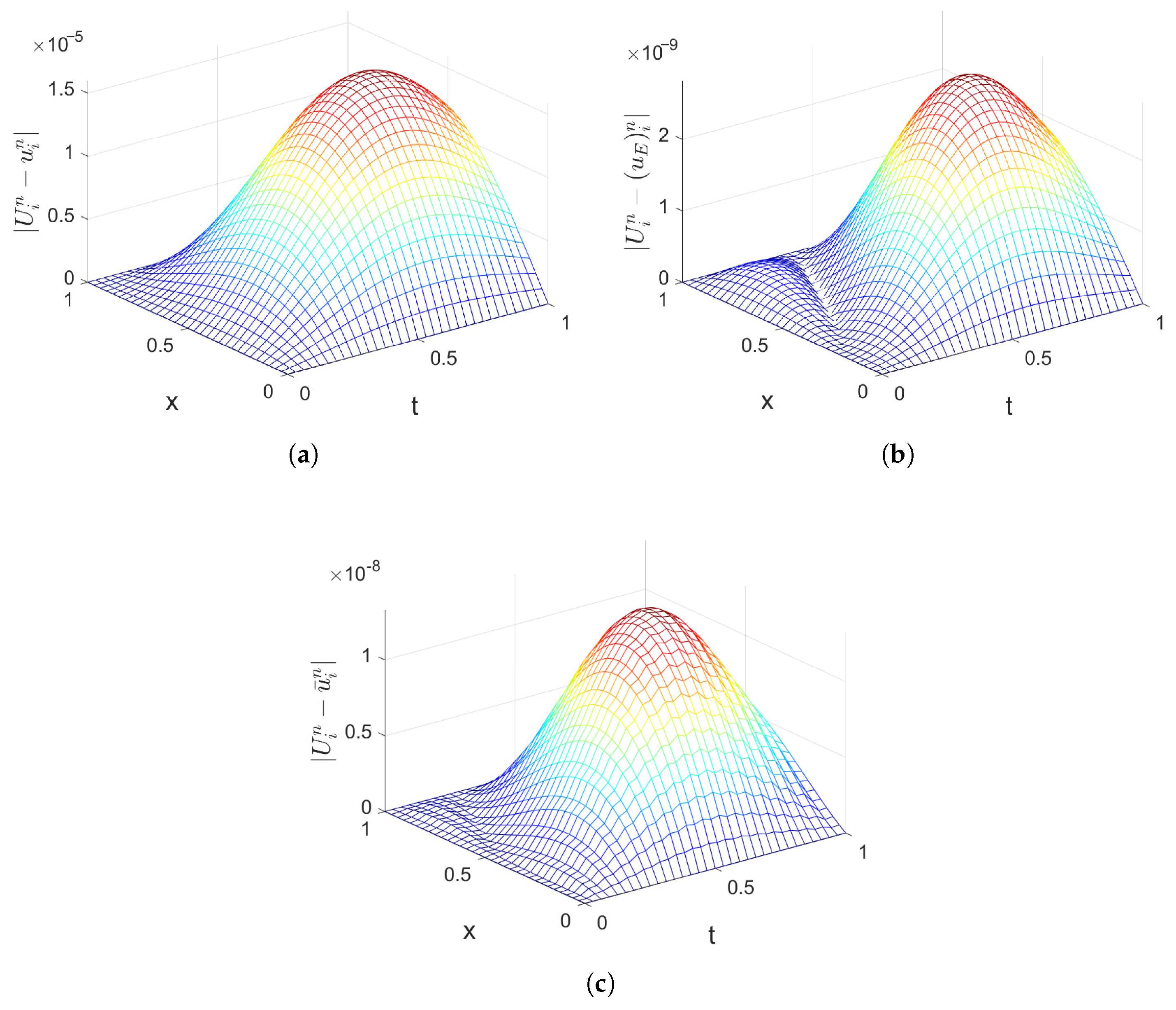
To verify the temporal convergence orders of Algorithms 1–3, we solve Example 1 using these algorithms with a fixed spatial step size ( h = 1 / 100 ) and varying temporal step sizes ( τ = 1 4 × i ) for ( i = 2 , 3 , 4 , 5 , 6 ) . The corresponding global errors and temporal convergence orders are presented in Table 1. As observed from Table 1, Algorithm 1 has second-order accuracy in time, while Algorithms 2 and 3 have fourth-order accuracies in time. Subsequently, to examine the spatial convergence orders, we fix the temporal step size at τ = 1 20 , 000 and the spatial step size is h = 1 4 × i for ( i = 2 , 3 , 4 , 5 , 6 ) . The computed results are summarized in Table 2, which shows that all three algorithms exhibit fourth-order spatial accuracies. Since Algorithms 1–3 employ the same discretization method as that for the second-order spatial derivatives, their spatial errors are comparable. Furthermore, Figure 1b–d illustrates the numerical solutions obtained using Algorithms 1–3, respectively, and, visually, they are almost indistinguishable from the exact solution plotted in Figure 1a. The corresponding global error surfaces are depicted in Figure 2a–c. It was found that the global errors of Algorithms 1–3 were 10 5 , 10 9 , and 10 8 , respectively.
Example 2.
Consider the following IBVPs of SLSEs:
u t u x x t = u x x + u ( 1 u ) + g ( x , t ) , x ( 0 , 1 ) , t ( 0 , 1 ] , u ( x , 0 ) = 0 , x [ 0 , 1 ] , u ( 0 , t ) = t 3 + t , u ( 1 , t ) = 0 , t ( 0 , 1 ] .
where
g ( x , t ) = ( π 2 4 + 1 ) ( 3 t 2 + 1 ) cos ( π 2 x ) ( 1 π 2 4 ) ( t 3 + t ) cos ( π 2 x ) + ( t 3 + t ) 2 cos 2 ( π 2 x )
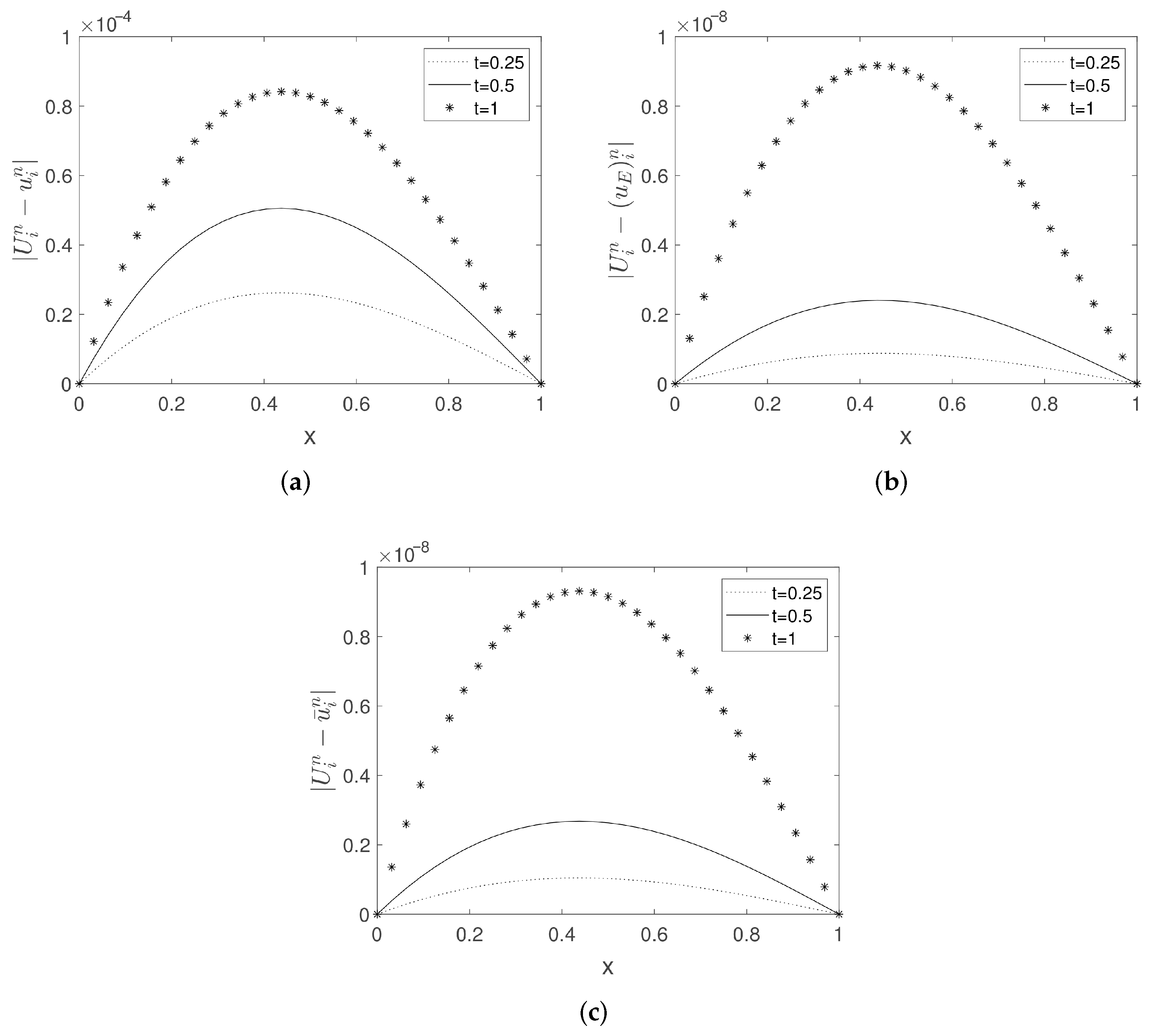
Example 2 admits a sufficiently smooth exact solution ( u ( x , t ) = ( t 3 + t ) cos ( π 2 x ) ). Table 3 presents the global errors and convergence orders for the numerical methods in reference [18] (denoted as Algorithm 4), as well as for Algorithms 2 and 3. Since Algorithm 4 is second-order accurate in time and fourth-order accurate in space, it is implemented with τ = h 2 to balance the temporal and spatial discretization errors. The results in Table 3 indicate that Algorithms 2 and 3 achieve fourth-order accuracies in both time and space, while Algorithm 4 maintains second-order temporal accuracy and fourth-order spatial accuracy. Furthermore, Algorithms 2 and 3 produce significantly smaller errors compared to those produced by Algorithm 4, indicating their superior performance. In addition, we solve Example 2 using Algorithms 1–3 with τ = h = 1 32 . The global errors at different time levels are plotted in Figure 3a–c. These figures further confirm that all three algorithms maintain high accuracy for Example 2.

6. Conclusions

In this paper, we have proposed a class of HOCDMs for solving SLSEs. A two-level scheme was first constructed using the C-N method in time and a fourth-order compact difference scheme in space, which has second-order temporal and fourth-order spatial accuracies. To further improve the time accuracy, the Richardson extrapolation technique was employed, successfully improving the temporal accuracy from second to fourth order. Moreover, a fully fourth-order accurate scheme in both time and space was developed by applying fourth-order discretizations to both temporal and spatial derivatives. And the convergence was also analyzed. Finally, numerical experiments were provided to confirm the accuracy and efficiency of the proposed methods.

Author Contributions

G.D. defined the research theme. T.W. designed numerical method. B.H. and Z.W. conducted the theory analysis and numerical experiments and wrote the paper. All authors have read and agreed to the published version of the manuscript.

Funding

This work is also supported by the Key Scientific Research Projects of Universities in Henan Province (26A110004), the Humanities and Social Science Foundation of the Ministry of Education of China (23YJCGJW008), the Henan Provincial Science and Technology Department Project (242400411163), and the Major Project of Philosophy and Social Research in Colleges and Universities of Henan Province (2025-YYZD-10).

Data Availability Statement

Data are contained within the article.

Acknowledgments

The authors gratefully acknowledge the anonymous reviewers for their insightful comments and valuable suggestions, which have significantly improved the quality of this manuscript.

Conflicts of Interest

The authors declare no conflicts of interest.

References

  1. Barenblatt, G.; Zheltov, I.; Kochina, I. Basic concepts in the theory of seepage of homogeneous liquids in fissured rocks. J. Appl. Math. Mech. 1960, 24, 1286–1303. [Google Scholar] [CrossRef]
  2. Shi, D. On the initial boundary value problem of nonlinear the equation of the migratiion of the moisture in soil. Acta Math. Appl. Sin. 1990, 13, 31–38. [Google Scholar]
  3. Ting, T.W. A cooling process according to two-temperature theory of heat conduction. J. Math. Anal. Appl. 1974, 45, 23–31. [Google Scholar] [CrossRef]
  4. Gu, H. Characteristic finite element methods for nonlinear sobolev equations. Appl. Math. Comput. 1999, 102, 51–62. [Google Scholar] [CrossRef]
  5. Gao, F.; Cui, J.; Zhao, G. Weak galerkin finite element methods for sobolev equation. J. Comput. Appl. Math. 2017, 317, 188–202. [Google Scholar] [CrossRef]
  6. Tran, T.; Duong, T.B. A posteriori error estimates with the finite element method of lines for a sobolev equation. Numer. Meth. Partial Differ. Equ. 2005, 21, 521–535. [Google Scholar] [CrossRef]
  7. Zeng, Y.; Luo, Z. The reduced-dimension technique for the unknown solution coefficient vectors in the Crank-Nicolson finite element method for the sobolev equation. J. Math. Anal. Appl. 2022, 513, 126207. [Google Scholar] [CrossRef]
  8. Abbaszadeh, M.; Dehghan, M. Interior penalty discontinuous Galerkin technique for solving generalized Sobolev equation. Appl. Numer. Math. 2020, 154, 172–186. [Google Scholar] [CrossRef]
  9. Wang, J.; Li, Q. Superconvergence analysis of a linearized three-step backward differential formula finite element method for nonlinear Sobolev equation. Math. Meth. Appl. Sci. 2019, 42, 3359–3376. [Google Scholar] [CrossRef]
  10. Xu, Y.; Zhou, Z.; Zhao, J. Conforming Virtual Element Methods for Sobolev Equations. J. Sci. Comput. 2022, 93, 32. [Google Scholar] [CrossRef]
  11. Liu, W.; Chen, Y.P.; Liang, Q. Unified analysis of conforming and nonconforming virtual element methods for nonlinear Sobolev equations. Calcolo 2025, 62, 7. [Google Scholar] [CrossRef]
  12. Tang, S.; Li, H.; Yin, B. A space-time spectral method for multi-dimensional Sobolev equations. J. Math. Anal. Appl. 2021, 499, 124937. [Google Scholar] [CrossRef]
  13. Jin, S.; Luo, Z. A collocation spectral method for two-dimensional Sobolev equations. Bound. Value Probl. 2018, 2018, 83. [Google Scholar] [CrossRef]
  14. Dehghan, M.; Shafieeabyaneh, N.; Shafieeabyaneh, M. Application of spectral element method for solving Sobolev equations with error estimation. Appl. Numer. Math. 2020, 158, 439–462. [Google Scholar] [CrossRef]
  15. Kumar, R.; Baskar, S. B-spline quasi-interpolation based numerical methods for some sobolev type equations. J. Comput. Appl. Math. 2016, 292, 41–66. [Google Scholar] [CrossRef]
  16. Yu, X.; Wang, M. Efficient spectral and spectral element methods for Sobolev equation with diagonalization technique. Appl. Numer. Math. 2024, 201, 265–281. [Google Scholar] [CrossRef]
  17. Dehghan, M.; Hooshyarfarzin, B.; Abbaszadeh, M. Proper orthogonal decomposition Pascal polynomial-based method for solving Sobolev equation. Int. J. Numer. Methods Heat Fluid Flow. 2022, 32, 2506–2542. [Google Scholar] [CrossRef]
  18. Chen, X.L.; Duan, J.Q.; Li, D.F. A newton linearized compact finite difference scheme for one class of sobolev equations. Numer. Meth. Partial Differ. Equ. 2018, 34, 1093–1112. [Google Scholar] [CrossRef]
  19. Zhang, Q.F.; Qin, Y.F.; Sun, Z.Z. Linearly compact scheme for 2D sobolev equation with burgers’s type nonlinearity. Numer. Algorithms 2022, 91, 1081–1114. [Google Scholar] [CrossRef]
  20. Li, X.; Rui, H. A block-centered finite difference method for the nonlinear Sobolev equation on nonuniform rectangular grids. Appl. Math. Comput. 2019, 363, 124607. [Google Scholar] [CrossRef]
  21. Xia, H.; Luo, Z.D. An optimized finite difference Crank-Nicolson iterative scheme for the 2D Sobolev equation. Adv. Differ. Equ. 2017, 2017, 196. [Google Scholar] [CrossRef]
  22. Wang, X.; Fu, H.F. Two linearized second-order block-centered finite difference methods for nonlinear Sobolev equations. Comput. Appl. Math. 2023, 42, 222. [Google Scholar] [CrossRef]
  23. Haq, S.; Ali, I. Approximate solution of two-dimensional Sobolev equation using a mixed Lucas and Fibonacci polynomials. Eng. Comput. 2022, 38, S2059–S2068. [Google Scholar] [CrossRef]
  24. Mishra, S.; Pany, A. Completely discrete schemes for 2D Sobolev equations with Burgers’ type nonlinearity. Numer. Algorithms 2022, 90, 963–987. [Google Scholar] [CrossRef]
  25. Singh, A.; Cheng, H.; Kumar, N.; Jiwari, R. A high order numerical method for analysis and simulation of 2D semilinear Sobolev model on polygonal meshes. Math. Comput. Simul. 2025, 227, 241–262. [Google Scholar] [CrossRef]
  26. Chen, H.; Nikan, O.; Qiu, W.; Avazzadeh, Z. Two-grid finite difference method for 1D fourth-order Sobolev-type equation with Burgers’ type nonlinearity. Math. Comput. Simul. 2023, 209, 248–266. [Google Scholar] [CrossRef]
  27. Zhang, J.; Qin, Y.F.; Zhang, Q.F. Maximum error estimates of two linearized compact difference schemes for two-dimensional nonlinear Sobolev equations. Appl. Numer. Math. 2023, 184, 253–272. [Google Scholar] [CrossRef]
  28. Hirsh, R.S. Higher order accurate difference solutions of fluid mechanics problems by a compact differencing technique. J. Comput. Phys. 1975, 19, 90–109. [Google Scholar] [CrossRef]
  29. Li, Q.Y.; Wang, N.C.; Yi, D.Y. Numerical Analysis; Tsinghua University Pres: Beijing, China, 2008. [Google Scholar]
  30. Sun, Z.Z. Numerical Solutions of Partial Differential Equations; Science Press: Beijing, China, 2012. [Google Scholar]
  31. Sun, Z.Z.; Zhang, Z.B. A linearized compact difference scheme for a class of nonlinear delay partial differential equations. Appl. Math. Model. 2013, 37, 742–752. [Google Scholar] [CrossRef]
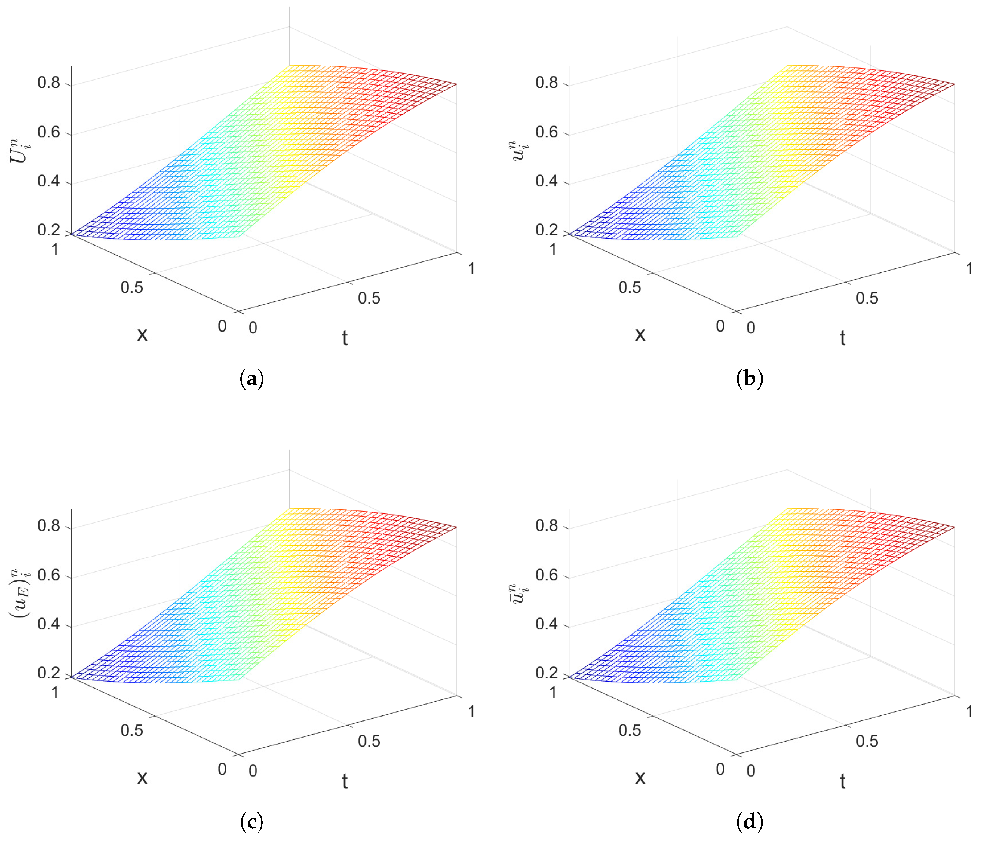
Figure 1. (a) Exact solution for Example 1; (b) Algorithm 1’s numerical solution for Example 1 ( τ = h = 1 32 ); (c) Algorithm 2’s numerical solution for Example 1 ( τ = h = 1 32 ); (d) Algorithm 3’s numerical solution for Example 1 ( τ = h = 1 32 ).
Axioms 14 00646 g001
Figure 2. (a) Global error surface of Algorithm 1 ( τ = h = 1 32 ); (b) Global error surface of Algorithm 2 ( τ = h = 1 32 ); (c) Global error surface of Algorithm 3 ( τ = h = 1 32 ).
Axioms 14 00646 g002
Figure 3. (a) Algorithm 1’s global errors for Example 2 ( τ = h = 1 32 ); (b) Algorithm 2’s global errors for Example 2 ( τ = h = 1 32 ); (c) Algorithm 3’s global errors for Example 2 ( τ = h = 1 32 ).
Axioms 14 00646 g003
Table 1. When h = 1 100 , the global errors and temporal convergence orders of Example 1.
τ Algorithm 1Algorithm 2Algorithm 3
E p τ E p τ E p τ
1 / 8 2.4000 × 10 3 2.2309 × 10 5 4.1279 × 10 4
1 / 12 1.0000 × 10 3 2.054.2737 × 10 6 4.085.5682 × 10 5 4.94
1 / 16 5.7672 × 10 4 2.021.3382 × 10 6 4.041.5581 × 10 5 4.43
1 / 20 3.6789 × 10 4 2.015.4221 × 10 7 4.026.5961 × 10 6 3.85
1 / 24 2.5503 × 10 4 2.012.6240 × 10 7 4.012.8509 × 10 6 4.60
Table 2. When τ = 1 20000 , the global errors and spatial convergence orders of Example 1.
hAlgorithm 1Algorithm 2Algorithm 3
E p h E p h E p h
1 / 8 4.7675 × 10 7 4.7711 × 10 7 4.7711 × 10 7
1 / 12 9.3562 × 10 8 4.029.3928 × 10 8 4.019.3929 × 10 8 4.01
1 / 16 2.9319 × 10 8 4.032.9654 × 10 8 4.012.9681 × 10 8 4.00
1 / 20 1.1783 × 10 8 4.091.2155 × 10 8 4.001.2152 × 10 8 4.00
1 / 24 5.4931 × 10 9 4.195.8431 × 10 9 4.025.8620 × 10 9 4.00
Table 3. Global errors and convergence orders of Example 2.
τ Algorithm 4 ( τ = h 2 ) Algorithm 2 ( τ = h )Algorithm 3 ( τ = h )
E p E p E p
1 / 5 3.4186 × 10 5 1.5330 × 10 5 1.5263 × 10 5
1 / 10 2.2410 × 10 6 3.939.5549 × 10 7 4.009.7483 × 10 7 3.97
1 / 20 1.4007 × 10 7 4.006.0070 × 10 8 3.996.1049 × 10 8 4.00
1 / 40 8.7545 × 10 9 4.003.7538 × 10 9 4.003.8101 × 10 9 4.00
Disclaimer/Publisher’s Note: The statements, opinions and data contained in all publications are solely those of the individual author(s) and contributor(s) and not of MDPI and/or the editor(s). MDPI and/or the editor(s) disclaim responsibility for any injury to people or property resulting from any ideas, methods, instructions or products referred to in the content.