The Unit Inverse Maxwell–Boltzmann Distribution: A Novel Single-Parameter Model for Unit-Interval Data

Abstract

The Unit Inverse Maxwell–Boltzmann (UIMB) distribution is introduced as a novel single-parameter model for data constrained within the unit interval ($0,1$), derived through an exponential transformation of the Inverse Maxwell–Boltzmann distribution. Designed to address the limitations of traditional unit-interval distributions, the UIMB model exhibits flexible density shapes and hazard rate behaviors, including right-skewed, left-skewed, unimodal, and bathtub-shaped patterns, making it suitable for applications in reliability engineering, environmental science, and health studies. This study derives the statistical properties of the UIMB distribution, including moments, quantiles, survival, and hazard functions, as well as stochastic ordering, entropy measures, and the moment-generating function, and evaluates its performance through simulation studies and real-data applications. Various estimation methods, including maximum likelihood, Anderson–Darling, maximum product spacing, least-squares, and Cramér–von Mises, are assessed, with maximum likelihood demonstrating superior accuracy. Simulation studies confirm the model’s robustness under normal and outlier-contaminated scenarios, with MLE showing resilience across varying skewness levels. Applications to manufacturing and environmental datasets reveal the UIMB distribution’s exceptional fit compared to competing models, as evidenced by lower information criteria and goodness-of-fit statistics. The UIMB distribution’s computational efficiency and adaptability position it as a robust tool for modeling complex unit-interval data, with potential for further extensions in diverse domains.

1. Introduction

Statistical modeling of data constrained within the unit interval (0, 1), encompassing proportions, ratios, and normalized concentrations, is a critical endeavor across diverse disciplines such as reliability engineering, environmental science, and health studies. These data types are prevalent in applications ranging from failure rate assessments to pollutant concentration analyses, necessitating robust distributional frameworks. Traditional models like the beta [1], Topp–Leone [2], and power distributions [3] have historically provided flexible tools for capturing a variety of shapes, from symmetric to highly skewed patterns. However, the escalating complexity of modern datasets, characterized by pronounced asymmetry, varying skewness, and non-monotonic hazard rate behaviors, has exposed limitations in these conventional approaches, driving the demand for innovative unit-interval distributions to improve fitting precision and interpretative depth [4,5,6].

The Maxwell–Boltzmann distribution (MB distribution), initially formulated by James Clerk Maxwell in 1867 to describe the velocity distribution of particles in an ideal gas [7], represents a cornerstone in statistical physics. Over time, the utility of the MB distribution has extended to reliability and lifetime data analysis, where the probability density function, defined over positive real values, proves effective for unbounded data modeling [8,9,10]. Despite these advancements, many real-world phenomena, such as normalized pollutant levels and reliability metrics, are inherently bounded within (0, 1), necessitating adaptive transformations. The Unit Maxwell–Boltzmann distribution (UMB distribution), derived through an exponential transformation of the MB distribution, has emerged as a valuable tool for modeling air pollutant concentrations, effectively addressing skewed data patterns in environmental studies [11,12].

In contrast, the Inverse Maxwell–Boltzmann distribution (InvMB distribution), introduced as the reciprocal of a random variable following the MB distribution, offers a distinctive upside-down bathtub (UBT)-shaped hazard rate, making it particularly suitable for lifetime data exhibiting non-monotonic failure behaviors [13,14]. Pioneered by Singh and Srivastava [15], the InvMB distribution has been rigorously tested with datasets like the GAGurine data, which display increasing-then-decreasing hazard profiles, a feature validated through stochastic ordering properties [16,17]. The applicability of the InvMB distribution is further enhanced by moment-based characterizations and quantile analyses [18]. However, the support of the InvMB distribution on the positive real line poses a significant challenge in its direct application to unit-interval data, limiting its adaptability to bounded domains [19,20].

To address this challenge, we propose the Unit Inverse Maxwell–Boltzmann distribution (UIMB distribution), a novel single-parameter model obtained by applying an exponential transformation to the InvMB distribution, restricting its support to (0, 1). This approach builds on the transformation framework established for the UMB distribution, retaining the flexible hazard rate properties of the InvMB distribution while adapting to bounded datasets. The UIMB distribution is specifically designed to model asymmetric or skewed data, providing a computationally efficient alternative to multi-parameter models.

This study systematically derives the UIMB distribution, investigates its statistical properties, including moments, quantiles, hazard, and survival functions, stochastic ordering, and entropy measures, and validates its efficacy through simulation studies and real-data applications. The simulation studies assess the model’s robustness under normal and outlier-contaminated scenarios, demonstrating its adaptability across varying levels of skewness and data contamination. Real-data applications further confirm its superior fit in manufacturing and environmental contexts. The paper is organized as follows: Section 2 defines the UIMB distribution, Section 3 examines its statistical characteristics, and Section 4 provides estimation methods of the model parameter. Section 5 outlines simulation settings and results, Section 6 provides real-data applications, and Section 7 concludes with future research directions.

2. Description of the Model

The UIMB distribution emerges as a single-parameter probability model designed to address the modeling of data constrained within the unit interval ($0,1$), a need highlighted by the limitations of unbounded distributions in contemporary applications. Building on the InvMB distribution, which is defined over the positive real line, the UIMB distribution is derived through an exponential transformation to accommodate bounded data, extending the methodological framework established for the UMB distribution. This transformation reflects a broader trend in statistical modeling toward adapting physical distributions for specialized datasets [21].

The UIMB distribution is obtained via the transformation $Y=e^{-X}$, where X follows an InvMB distribution with parameter $\theta$. The choice of the exponential transformation is theoretically justified by its ability to map the unbounded positive support of X to the bounded unit interval (0, 1) while preserving essential probabilistic properties, such as the non-monotonic hazard rate behavior. This transformation is rooted in statistical physics, where exponential mappings naturally arise in modeling decay processes or normalized concentrations, aligning with the Maxwell–Boltzmann heritage. Alternative transformations for generating unit-interval distributions from unbounded ones include the logistic transformation, which yields a symmetric sigmoid shape but may over-smooth asymmetries, the probit transformation using the normal CDF, suitable for Gaussian-based models but less flexible for skewed data, or fractional transformations, which can introduce heavier tails but complicate hazard interpretations. The exponential transformation is preferred here over these alternatives because it maintains the InvMB’s UBT hazard rate—characterized by an initial increase followed by a decrease—while inverting it appropriately for the unit interval, making it ideal for reliability data with early failures and later stabilization. In contrast, logistic or probit alternatives often result in monotonic hazards, limiting their applicability to non-monotonic patterns observed in real datasets. The probability density function (PDF) of the UIMB distribution with parameter $\theta$ is given by

$$f_Y(y;\theta )={\displaystyle \frac{4}{\sqrt{\pi }{\theta }^{3/2}y{log}^{4}y}}exp\left(-{\displaystyle \frac{1}{\theta {log}^{2}y}}\right),\hspace{1em}0<y<1,\hspace{1em}\theta >0.$$

(1)

The corresponding cumulative distribution function (CDF) is

$$F_Y(y;\theta )=1-{\displaystyle \frac{2}{\sqrt{\pi }}}\mathsf{\Gamma }\left({\displaystyle \frac{3}{2}},{\displaystyle \frac{1}{\theta {log}^{2}y}}\right),0<y<1,$$

(2)

where $\theta >0$ is the scale parameter and $\mathsf{\Gamma }(a,z)={\mathit{\int }}_z^{\infty }{t}^{a-1}{e}^{-t}dt,a>0,z>0$ denotes the upper incomplete gamma function. The survival function (SF) and hazard rate function (HRF) are, respectively,

$$S_Y(y;\theta )={\displaystyle \frac{2}{\sqrt{\pi }}}\mathsf{\Gamma }\left({\displaystyle \frac{3}{2}},{\displaystyle \frac{1}{\theta {log}^{2}y}}\right),0<y<1,$$

(3)

$$H_Y(y;\theta )={\displaystyle \frac{2}{{\theta }^{3/2}y{log}^{4}y}}{\displaystyle \frac{exp\left(-\frac{1}{\theta {log}^{2}y}\right)}{\mathsf{\Gamma }\left(\frac{3}{2},\frac{1}{\theta {log}^{2}y}\right)}},0<y<1.$$

(4)

The UIMB distribution exhibits a range of density shapes, including right-skewed, left-skewed, and unimodal forms, modulated by the parameter $\theta$. These shape properties are visualized in Figure 1. The first row of Figure 1 displays the PDF (1) and CDF (2) for various $\theta$ values, illustrating the flexibility of the UIMB distribution in modeling unit-interval data. The second row displays the HRF (4), which reveals diverse hazard profiles, including increasing and bathtub-like shapes, ideal for reliability applications. With its single-parameter design, the UIMB distribution balances computational efficiency and modeling flexibility. Its foundation with bounded support makes it particularly suitable for applications requiring precise modeling of unit-interval phenomena.

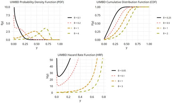
Figure 1. Plots of the PDF (top left), CDF (top right), and HRF (bottom) of the UIMB distribution for various $\theta$ values.

3. Some Statistical Characteristics

This section explores key statistical properties of the UIMB distribution, providing a comprehensive analysis of its quantile function, moments, and reliability characteristics. These properties elucidate the behavior of the distribution and its applicability to modeling unit-interval data across various domains.

3.1. Quantile Function

The quantile function of the UIMB distribution facilitates random number generation and offers valuable insights into the behavior of the distribution across probability levels. For a random variable Y following a UIMB distribution with parameter $\theta$, the quantile function $Q(p;\theta )$ is expressed as

$$Q(p;\theta )=exp\left(-{\displaystyle \frac{1}{\sqrt{\theta {\mathsf{\Gamma }}^{-1}\left(\frac{3}{2},\frac{\sqrt{\pi }}{2}(1-p)\right)}}}\right),p\in (0,1).$$

(5)

Table 1 presents numerical quantile values for various $\theta$ values and probability levels, illustrating the adaptability of the UIMB distribution to different data scenarios. The table shows that as $\theta$ increases from 0.1 to 100, the quantiles shift toward higher values, reflecting a rightward shift in the mass of the distribution. This trend highlights the flexibility of UIMB distribution in modeling data with varying central tendencies within the unit interval.

Table 1. Computed quantile values of the UIMB distribution for various values of $\theta$ and probability levels.

$\mathit{\theta }$	Q (0.05)	Q (0.1)	Q (0.2)	Q (0.3)	Q (0.5)	Q (0.7)	Q (0.9)	Q (0.99)	Q (0.999)
0.1	0.0005	0.0029	0.0116	0.0236	0.0546	0.0967	0.1672	0.2651	0.3299
0.5	0.0343	0.0731	0.1360	0.1871	0.2725	0.3518	0.4494	0.5522	0.6090
1	0.0922	0.1572	0.2440	0.3057	0.3988	0.4777	0.5680	0.6571	0.7042
2	0.1853	0.2703	0.3688	0.4325	0.5220	0.5931	0.6703	0.7431	0.7804
5	0.3443	0.4372	0.5322	0.5886	0.6629	0.7187	0.7765	0.8288	0.8549
10	0.4705	0.5571	0.6401	0.6874	0.7477	0.7917	0.8362	0.8757	0.8950
25	0.6208	0.6907	0.7542	0.7890	0.8320	0.8627	0.8930	0.9195	0.9323
50	0.7138	0.7698	0.8192	0.8457	0.8781	0.9008	0.9231	0.9423	0.9516
100	0.7879	0.8311	0.8684	0.8882	0.9122	0.9288	0.9450	0.9589	0.9655

The quantile function enables random variate generation from the UIMB distribution using the inverse transform sampling method. The procedure is outlined as follows:

(1)

Set the scale parameter $\theta >0$ and the desired number of samples n.

(2)

For each $i=1$ to n:

(a)

Generate a random number $U_i\sim U(0,1)$.

(b)

Compute $Y_i=exp\left(-{\displaystyle \frac{1}{\sqrt{\theta {\mathsf{\Gamma }}^{-1}\left(\frac{3}{2},\frac{\sqrt{\pi }}{2}(1-U_i)\right)}}}\right)$.

(3)

Return the set of random samples $Y_1,Y_2,\dots ,Y_n$.

Furthermore, the UIMB distribution has transformation relationships with other distributions. Specifically, if $X\sim \mathrm{InvMB}\left(\theta \right)$, then $Y=e^{-X}\sim \mathrm{UIMB}\left(\theta \right)$. This relationship highlights the UIMB’s derivation from the InvMB distribution, extending its utility to bounded domains while preserving key probabilistic features.

3.2. Moments

The r-th moment of the random variable Y following a UIMB distribution with parameter $\theta$ is given by

$$E\left(Y^r\right)={\mathit{\int }}_0^1{y}^r{f}_Y(y;\theta )dy={\displaystyle \frac{4}{\sqrt{\pi }{\theta }^{3/2}}}{\mathit{\int }}_0^1{y}^{r-1}{\displaystyle \frac{1}{{log}^{4}y}}exp\left(-{\displaystyle \frac{1}{\theta {log}^{2}y}}\right)dy.$$

(6)

To simplify the integral in Equation (6), we apply the substitution $v=1/{log}^{2}y$, which transforms the expression to

$$E\left(Y^r\right)={\displaystyle \frac{2}{\sqrt{\pi }{\theta }^{3/2}}}{\mathit{\int }}_0^{\infty }{v}^{1/2}exp\left(-{\displaystyle \frac{r}{\sqrt{v}}}-{\displaystyle \frac{v}{\theta }}\right)dv.$$

(7)

The moments in Equation (7) can be expressed analytically using the Meijer G-function, a generalized hypergeometric function useful for integrals involving exponential and power terms. Specifically, the integral ${\mathit{\int }}_0^{\infty }{x}^{a-1}exp(-bx-c/x)dx$ can be expressed as $2{(c/b)}^{a/2}{K}_{-a}\left(2\sqrt{bc}\right)$, where $K_a$ is the modified Bessel function of the second kind, which is equivalent to $G_{0,3}^{3,0}(z|0,{\displaystyle \frac{a-1}{2}},{\displaystyle \frac{a+1}{2}})$ up to constants, where

$$G_{p,q}^{m,n}\left(z\right|a_1,\dots ,a_p;b_1,\dots ,b_q)={\displaystyle \frac{1}{2\pi i}}{\mathit{\int }}_L{\displaystyle \frac{{\prod }_{j=1}^m\mathsf{\Gamma }(b_j+s){\prod }_{j=1}^n\mathsf{\Gamma }(1-a_j-s)}{{\prod }_{j=m+1}^q\mathsf{\Gamma }(1-b_j-s){\prod }_{j=n+1}^p\mathsf{\Gamma }(a_j+s)}}{z}^{-s}ds$$

is the Meijer G-function [22]. Hence, with $a=3/2$, $b=1/\theta$, $c=r^2/4$ in Equation (7), we obtain that

$$E\left(Y^r\right)={\displaystyle \frac{2}{\pi }}{G}_{0,3}^{3,0}\left({\displaystyle \frac{r^2}{4\theta }}|\begin{array}{c}0,{\displaystyle \frac{1}{2}},{\displaystyle \frac{3}{2}}\end{array}\right).$$

(8)

Equation (8) provides a closed-form expression for the moments of the UIMB distribution, enabling precise computation. The first four moments ($r=1,2,3,4$), variance, skewness, and kurtosis of the UIMB distribution are calculated for $\theta =0.1,0.2,\dots ,0.9,1,2,5,10,25,50$, and the results are presented in Table 2.

Table 2. Moments for $r=1,2,3,4$, variance, skewness, and kurtosis of the UIMB distribution for various $\theta$ values.

$\mathit{\theta }$	$\mathit{E}\left(\mathit{Y}\right)$	$\mathit{E}\left({\mathit{Y}}^2\right)$	$\mathit{E}\left({\mathit{Y}}^3\right)$	$\mathit{E}\left({\mathit{Y}}^4\right)$	Variance	Skewness	Kurtosis
0.1	0.0717	0.0094	0.0016	0.0003	0.0043	1.0691	0.7349
0.2	0.1405	0.0297	0.0075	0.0021	0.0100	0.5447	−0.4208
0.3	0.1926	0.0512	0.0158	0.0053	0.0141	0.2807	−0.7045
0.4	0.2340	0.0717	0.0250	0.0094	0.0170	0.1056	−0.7831
0.5	0.2680	0.0909	0.0345	0.0141	0.0191	−0.0251	−0.7843
0.6	0.2968	0.1087	0.0441	0.0192	0.0206	−0.1294	−0.7498
0.7	0.3216	0.1252	0.0535	0.0244	0.0217	−0.2162	−0.6969
0.8	0.3434	0.1405	0.0628	0.0297	0.0226	−0.2905	−0.6338
0.9	0.3628	0.1548	0.0717	0.0351	0.0232	−0.3555	−0.5650
1	0.3802	0.1682	0.0804	0.0405	0.0236	−0.4133	−0.4932
2	0.4936	0.2680	0.1533	0.0909	0.0243	−0.7904	0.2305
5	0.6300	0.4171	0.2845	0.1983	0.0202	−1.2972	1.9517
10	0.7165	0.5288	0.3977	0.3033	0.0154	−1.7015	4.0145
25	0.8063	0.6596	0.5450	0.4538	0.0094	−2.2800	8.2022
50	0.8573	0.7409	0.6442	0.5628	0.0060	−2.7601	12.9674

Table 2 illustrates the evolution of the statistical characteristics of the UIMB distribution as the parameter $\theta$ varies from 0.1 to 50. As $\theta$ increases, the first four moments grow steadily, shifting the mass of the distribution toward $y\to 1$. Variance peaks near $\theta \approx 2$, indicating maximal dispersion, and gradually declines for larger $\theta$, reflecting increasing concentration around the upper bound. Skewness values shift from strongly positive at small $\theta$ to negative for large $\theta$, with near symmetry observed around $\theta \approx 0.5$. This trend signals a transition from right-skewed to left-skewed behavior. Similarly, kurtosis evolves from moderate leptokurtic to platykurtic around $\theta \approx 0.5$, and finally to highly leptokurtic at large $\theta$, indicating the development of heavy tails. These patterns underscore the flexibility of the distribution in capturing both skewed and heavy-tailed behaviors across the unit interval.

3.3. Moment Generating Function

The moment-generating function (MGF) of a random variable Y following the UIMB distribution with parameter $\theta$ is defined as

$$M\left(t\right)=E\left(e^{tY}\right)={\mathit{\int }}_0^1{e}^{ty}{f}_Y(y;\theta )dy,t\in \mathbb{R}.$$

Expanding $e^{ty}={\sum }_{k=0}^{\infty }{\displaystyle \frac{{\left(ty\right)}^k}{k!}}$ allows one to express the MGF as

$$M\left(t\right)=\sum _{k=0}^{\infty }{\displaystyle \frac{t^k}{k!}}E\left(Y^k\right),$$

where the k-th moment $E\left(Y^k\right)$ is derived from Equation (8). Thus, the MGF can be written as

$$M\left(t\right)=\sum _{k=0}^{\infty }{\displaystyle \frac{2t^k}{\pi k!}}{G}_{0,3}^{3,0}\left({\displaystyle \frac{k^2}{4\theta }}|\begin{array}{c}0,{\displaystyle \frac{1}{2}},{\displaystyle \frac{3}{2}}\end{array}\right).$$

(9)

The series representation in Equation (9) enables numerical computation by truncating the series at a sufficient k, utilizing the Meijer G-function’s efficient evaluation in mathematical software such as Mathematica.

3.4. Stress–Strength Reliability

The stress–strength reliability model quantifies the probability that the strength of a system exceeds the applied stress. For the UIMB distribution, we consider $Y_1\sim \mathrm{UIMB}\left({\theta }_1\right)$ as the strength and $Y_2\sim \mathrm{UIMB}\left({\theta }_2\right)$ as the stress. Without loss of generality, we assume that ${\theta }_1<{\theta }_2$, then the stress–strength reliability is defined as

$$R={\mathit{\int }}_0^1{f}_{Y_1}(y_1;{\theta }_1)F_{Y_2}(y_1;{\theta }_2)d{y}_1.$$

(10)

Substituting the PDF (1) and CDF (2) of the UIMB distribution, we obtain

$$\begin{array}{cc}\hfill R& ={\mathit{\int }}_0^1\left[{\displaystyle \frac{4}{\sqrt{\pi }{\theta }_1^{3/2}}}{\displaystyle \frac{1}{y_1{log}^4{y}_1}}exp\left(-{\displaystyle \frac{1}{{\theta }_1{log}^2{y}_1}}\right)\right]\left[1-{\displaystyle \frac{2}{\sqrt{\pi }}}\mathsf{\Gamma }\left({\displaystyle \frac{3}{2}},{\displaystyle \frac{1}{{\theta }_2{log}^2{y}_1}}\right)\right]d{y}_1\hfill \\ \hfill & ={\displaystyle \frac{4}{\sqrt{\pi }{\theta }_1^{3/2}}}{\mathit{\int }}_0^1{\displaystyle \frac{1}{y_1{log}^4{y}_1}}exp\left(-{\displaystyle \frac{1}{{\theta }_1{log}^2{y}_1}}\right)\left[1-{\displaystyle \frac{2}{\sqrt{\pi }}}\mathsf{\Gamma }\left({\displaystyle \frac{3}{2}},{\displaystyle \frac{1}{{\theta }_2{log}^2{y}_1}}\right)\right]d{y}_1\hfill \end{array}$$

(11)

Apply the substitution $u=-log{y}_1$ in Equation (11) to obtain

$$R={\displaystyle \frac{4}{\sqrt{\pi }{\theta }_1^{3/2}}}{\mathit{\int }}_0^{\infty }{u}^{-4}exp\left(-{\displaystyle \frac{1}{{\theta }_1{u}^2}}\right)\left[1-{\displaystyle \frac{2}{\sqrt{\pi }}}\mathsf{\Gamma }\left({\displaystyle \frac{3}{2}},{\displaystyle \frac{1}{{\theta }_2{u}^2}}\right)\right]e^{-u}du.$$

(12)

Using the normalized incomplete gamma function $P(a,z)=1-Q(a,z)$, where $Q(a,z)={\displaystyle \frac{\mathsf{\Gamma }(a,z)}{\mathsf{\Gamma }\left(a\right)}}$ and the series expansion

$$\begin{array}{cc}\hfill 1-{\displaystyle \frac{2}{\sqrt{\pi }}}\mathsf{\Gamma }\left({\displaystyle \frac{3}{2}},{\displaystyle \frac{1}{{\theta }_2{u}^2}}\right)& =P\left({\displaystyle \frac{3}{2}},{\displaystyle \frac{1}{{\theta }_2{u}^2}}\right)\hfill \\ \hfill & ={\displaystyle \frac{2}{\sqrt{\pi }}}\sum _{k=0}^{\infty }{\displaystyle \frac{{(-1)}^k}{k!(k+3/2)}}{\left({\displaystyle \frac{1}{{\theta }_2{u}^2}}\right)}^k\hfill \end{array}$$

in Equation (12) yields

$$\begin{array}{cc}\hfill R& ={\displaystyle \frac{4}{\sqrt{\pi }{\theta }_1^{3/2}}}{\mathit{\int }}_0^{\infty }{u}^{-4}exp\left(-{\displaystyle \frac{1}{{\theta }_1{u}^2}}-u\right)·\left[{\displaystyle \frac{2}{\sqrt{\pi }}}\sum _{k=0}^{\infty }{\displaystyle \frac{{(-1)}^k}{k!(k+3/2)}}{\theta }_2^{-k}{u}^{-2k}\right]du\hfill \\ \hfill & ={\displaystyle \frac{8}{\pi {\theta }_1^{3/2}}}\sum _{k=0}^{\infty }{\displaystyle \frac{{(-1)}^k}{k!(k+3/2)}}{\theta }_2^{-k}{\mathit{\int }}_0^{\infty }{u}^{-2k-4}exp\left(-{\displaystyle \frac{1}{{\theta }_1{u}^2}}-u\right)du.\hfill \end{array}$$

(13)

Evaluate the inner integral in Equation (13) with $w={\displaystyle \frac{u^2}{{\theta }_1}}$, then the final form of the reliability is

$$R={\displaystyle \frac{4}{\pi }}{\left({\displaystyle \frac{{\theta }_1}{{\theta }_2}}\right)}^{3/2}\sum _{k=0}^{\infty }{\displaystyle \frac{{(-1)}^k(k+1)(k+2)}{k+3/2}}{\left({\displaystyle \frac{{\theta }_1}{{\theta }_2}}\right)}^k.$$

(14)

3.5. Stochastic Ordering Properties

To elucidate the behavior of the UIMB distribution, we explore its stochastic ordering properties by comparing two UIMB random variables with different parameters, $Y_1\sim \mathrm{UIMB}\left({\theta }_1\right)$ and $Y_2\sim \mathrm{UIMB}\left({\theta }_2\right)$, assuming ${\theta }_1<{\theta }_2$ without loss of generality. These properties, likelihood ratio order and hazard rate order, provide insights into the comparative behavior of random variables, particularly in reliability and risk analysis.

3.5.1. Likelihood Ratio Order

$Y_1$ is said to be smaller than $Y_2$ in the likelihood ratio order (denoted $Y_1{\le }_{\mathrm{lr}}{Y}_2$) if the ratio of their PDFs, $f_{Y_1}(y;{\theta }_1)/f_{Y_2}(y;{\theta }_2)$, is non-increasing in $y\in (0,1)$. Based on the PDF of the UIMB distribution given by Equation (1), the likelihood ratio is

$$\begin{array}{cc}\hfill r\left(y\right)& ={\left({\displaystyle \frac{{\theta }_2}{{\theta }_1}}\right)}^{3/2}exp\left(\left({\displaystyle \frac{1}{{\theta }_2}}-{\displaystyle \frac{1}{{\theta }_1}}\right){\displaystyle \frac{1}{{log}^{2}y}}\right)\hfill \\ \hfill & ={\left({\displaystyle \frac{{\theta }_2}{{\theta }_1}}\right)}^{3/2}exp\left(\left({\displaystyle \frac{1}{{\theta }_2}}-{\displaystyle \frac{1}{{\theta }_1}}\right)w\right)\hfill \end{array}$$

where $w=1/{(logy)}^2>0$. It can be easily shown that $r\left(y\right)$ is non-increasing in y for ${\theta }_1<{\theta }_2$. Therefore, $Y_1{\le }_{\mathrm{lr}}{Y}_2$ when ${\theta }_1<{\theta }_2$.

3.5.2. Hazard Rate Order

$Y_1{\le }_{\mathrm{hr}}{Y}_2$ if the hazard rate $H_{Y_1}(y;{\theta }_1)\ge H_{Y_2}(y;{\theta }_2)$ for all $y\in (0,1)$. Based on the hazard rate given by Equation (4), we obtain that

$$\begin{array}{cc}\hfill {\displaystyle \frac{H\left({\theta }_1\right)}{H\left({\theta }_2\right)}}& ={\left({\displaystyle \frac{{\theta }_2}{{\theta }_1}}\right)}^{3/2}{\displaystyle \frac{exp(-w/{\theta }_1)}{exp(-w/{\theta }_2)}}{\displaystyle \frac{\mathsf{\Gamma }(3/2,w/{\theta }_2)}{\mathsf{\Gamma }(3/2,w/{\theta }_1)}}\hfill \\ \hfill & ={\left({\displaystyle \frac{{\theta }_2}{{\theta }_1}}\right)}^{3/2}exp\left(w\left({\displaystyle \frac{1}{{\theta }_2}}-{\displaystyle \frac{1}{{\theta }_1}}\right)\right){\displaystyle \frac{\mathsf{\Gamma }(3/2,w/{\theta }_2)}{\mathsf{\Gamma }(3/2,w/{\theta }_1)}}\hfill \end{array}$$

where $w=1/{log}^{2}y>0$. The overall ratio depends on the balance: for small w (large y), the exponential dominates, suggesting $H\left({\theta }_1\right)<H\left({\theta }_2\right)$, while for large w (small y), the gamma ratio may dominate, suggesting $H\left({\theta }_1\right)>H\left({\theta }_2\right)$. Numerically, for ${\theta }_1=0.5$, ${\theta }_2=1$, $H\left({\theta }_1\right)>H\left({\theta }_2\right)$ near $y\to 0$ but reverses near $y\to 1$, indicating that the order is not universal without specific constraints.

3.6. Entropy Measures

Entropy measures quantify the uncertainty or information content of a probability distribution, providing insights into its randomness and predictability, which are valuable in applications such as reliability engineering and information theory. In this subsection, we derive the Shannon entropy for the UIMB distribution and discuss the Rényi and Tsallis entropies, which generalize the Shannon entropy for broader analytical purposes.

3.6.1. Shannon Entropy

The Shannon entropy for a continuous random variable Y with PDF $f_Y(y;\theta )$ is defined as

$$H\left(Y\right)=-{\mathit{\int }}_0^1{f}_Y(y;\theta )log{f}_Y(y;\theta )dy.$$

For the UIMB distribution, the Shannon entropy becomes

$$\begin{array}{cc}\hfill H\left(Y\right)& =-{\mathit{\int }}_0^1{f}_Y(y;\theta )\left[log4-{\displaystyle \frac{1}{2}}log\pi -{\displaystyle \frac{3}{2}}log\theta -logy-4log(-logy)-{\displaystyle \frac{1}{\theta {log}^{2}y}}\right]dy\hfill \\ \hfill & =-log4+{\displaystyle \frac{1}{2}}log\pi +{\displaystyle \frac{3}{2}}log\theta +{\mathit{\int }}_0^1{f}_Y(y;\theta )logydy+4{\mathit{\int }}_0^1{f}_Y(y;\theta )log(-logy)dy\hfill \\ \hfill & +{\mathit{\int }}_0^1{f}_Y(y;\theta ){\displaystyle \frac{1}{\theta {log}^{2}y}}dy\hfill \end{array}$$

(15)

where $f_Y(y;\theta )$ is the PDF of the UIMB distribution given by Equation (1). After applying the substitution $u=-logy$ in Equation (15), the Shannon entropy is obtained as

$$H\left(Y\right)=-log4+{\displaystyle \frac{1}{2}}log\pi +{\displaystyle \frac{3}{2}}log\theta -{\displaystyle \frac{2}{\sqrt{\pi }{\theta }^{1/2}}}+{\displaystyle \frac{9}{2}}.$$

3.6.2. Rényi and Tsallis Entropies

The Rényi entropy of order $\alpha$ (where $\alpha >0$, $\alpha \ne 1$) is defined as

$$H_{\alpha }\left(Y\right)={\displaystyle \frac{1}{1-\alpha }}log\left({\mathit{\int }}_0^1{\left[f_Y(y;\theta )\right]}^{\alpha }dy\right).$$

(16)

The Tsallis entropy of order $\alpha$ is

$$S_{\alpha }\left(Y\right)={\displaystyle \frac{1}{\alpha -1}}\left(1-{\mathit{\int }}_0^1{\left[f_Y(y;\theta )\right]}^{\alpha }dy\right).$$

(17)

Both of the entropies depends on the integral $I\left(\alpha \right)={\mathit{\int }}_0^1{\left[f_Y(y;\theta )\right]}^{\alpha }dy$, which can be expresses as

$$I\left(\alpha \right)={\displaystyle \frac{4^{\alpha }}{{\pi }^{\alpha /2}{\theta }^{3\alpha /2}}}{\mathit{\int }}_0^{\infty }{u}^{-4\alpha }exp\left((\alpha -1)u-{\displaystyle \frac{\alpha }{\theta u^2}}\right)du,$$

derived via the substitution $u=-logy$. For $\alpha >1$, the term $exp\left(\right(\alpha -1\left)u\right)$ causes divergence as $u\to \infty$, so $I\left(\alpha \right)=\infty$ and $H_{\alpha }\left(Y\right)\to -\infty$. This reflects the behavior of the distribution near $y\to 0^{+}$, where the PDF grows like $y^{-1}{log}^{-4}y$, leading to heavy-tailed higher powers.

For $\alpha <1$, the integral converges, and using the Meijer G-function representation we obtain that

$$I\left(\alpha \right)={\displaystyle \frac{{(1-\alpha )}^{-(1-4\alpha )}}{4^{\alpha }{\pi }^{(1+\alpha )/2}{\theta }^{3\alpha /2}}}{G}_{3,0}^{0,3}\left({\displaystyle \frac{4\theta }{{(1-\alpha )}^2\alpha }}|\begin{array}{c}1,2+2\alpha ,5/2+2\alpha \end{array}\right).$$

(18)

The closed-form of $I\left(\alpha \right)$ in Equation (18) enables computation of Renyi and Tsallis entropies for $\alpha <1$, which are given by Equations (16) and (17), respectively.

These entropy measures enhance the understanding of the information content of the UIMB distribution, with the Shannon entropy providing a precise analytical form, and the Rényi and Tsallis entropies offering Meijer G-based expressions for $\alpha <1$.

3.7. Order Statistics

Order statistics are essential in reliability engineering and quality control, where the smallest or largest values in a sample often indicate system failure points or quality thresholds. For an independent and identically distributed random sample $Y_1,Y_2,\dots ,Y_n$ from the UIMB distribution with parameter $\theta$, the PDF of the k-th order statistic $Y_{\left(k\right)}$ ($1\le k\le n$) is given by

$$\begin{array}{cc}\hfill f_{\left(k\right)}(y;\theta )& ={\displaystyle \frac{n!}{(k-1)!(n-k)!}}{\left[F_Y(y;\theta )\right]}^{k-1}{[1-F_Y(y;\theta )]}^{n-k}{f}_Y(y;\theta ),0<y<1,\hfill \\ \hfill & ={\displaystyle \frac{2^{n-k+2}}{{\theta }^{3/2}{\pi }^{(n-k+1)/2}}}{\displaystyle \frac{n!}{(k-1)!(n-k)!}}{\displaystyle \frac{1}{y{log}^{4}y}}{\left[1-{\displaystyle \frac{2}{\sqrt{\pi }}}\mathsf{\Gamma }\left({\displaystyle \frac{3}{2}},{\displaystyle \frac{1}{\theta {log}^{2}y}}\right)\right]}^{k-1}\hfill \\ \hfill & \times {\left[\mathsf{\Gamma }\left({\displaystyle \frac{3}{2}},{\displaystyle \frac{1}{\theta {log}^{2}y}}\right)\right]}^{n-k}exp\left(-{\displaystyle \frac{1}{\theta {log}^{2}y}}\right)\hfill \end{array}$$

where $f_Y(y;\theta )$ is the PDF from Equation (1) and $F_Y(y;\theta )$ is the CDF from Equation (2).

The form of the r-th moment of the k-th order statistic is complex due to the incomplete gamma function in $F_Y(y;\theta )$, and the corresponding integral does not yield a closed-form expression in terms of elementary or standard special functions. Numerical evaluation can be performed via quadrature methods or Monte Carlo simulation, where samples are generated using the quantile function from Equation (5) and ordered to compute the moments. In reliability applications, these moments are useful for estimating expected failure times, such as $E\left(Y_{\left(1\right)}\right)$ for the minimum lifetime in parallel systems or $E\left(Y_{\left(n\right)}\right)$ for the maximum lifetime in series systems.

4. Estimation Methods

This section examines various classical approaches for estimating the scale parameter $\theta$ of the UIMB distribution. Given a random sample $y_1,y_2,\dots ,y_n$ from the UIMB distribution with scale parameter $\theta$, we investigate maximum likelihood estimation (MLE), Anderson–Darling (AD), maximum product spacing (MPS), ordinary least-squares (OLS), weighted least-squares (WLS), and Cramér-von Mises (CVM) methods. These methods provide reliable parameter estimation for unit-interval data, with numerical optimization often necessitated by the nonlinear nature of the incomplete gamma function within the structure of the UIMB distribution.

4.1. Maximum Likelihood Estimation

The maximum likelihood estimator (MLE) for $\theta$ is obtained by maximizing the log-likelihood function

$$\ell \left(\theta \right)=logL\left(\theta \right)=log4n-log\sqrt{\pi }n-{\displaystyle \frac{3}{2}}nlog\theta -\sum _{i=1}^{n}log{y}_i-4\sum _{i=1}^{n}log(-log{y}_i)-\sum _{i=1}^n{\displaystyle \frac{1}{\theta {log}^2{y}_i}}.$$

(19)

Differentiating Equation (19) with respect to $\theta$, we get

$${\displaystyle \frac{\partial \ell \left(\theta \right)}{\partial \theta }}=-{\displaystyle \frac{3n}{2\theta }}+\sum _{i=1}^n{\displaystyle \frac{1}{{\theta }^2\left({log}^2{y}_i\right)}}=0.$$

(20)

The closed-form solution for the MLE is

$${\widehat{\theta }}_{\mathrm{MLE}}={\displaystyle \frac{2}{3n}}\sum _{i=1}^n{\displaystyle \frac{1}{\left({log}^2{y}_i\right)}}.$$

(21)

To establish the existence and uniqueness of the MLE, consider the second derivative of the log-likelihood function

$${\displaystyle \frac{{\partial }^2\ell \left(\theta \right)}{\partial {\theta }^2}}={\displaystyle \frac{3n}{2{\theta }^2}}-2\sum _{i=1}^n{\displaystyle \frac{1}{{\theta }^3{log}^2{y}_i}}.$$

(22)

The second derivative in Equation (22) is negative when ${\displaystyle \frac{3n}{2{\theta }^2}}<2{\sum }_{i=1}^n{\displaystyle \frac{1}{{\theta }^3\left({log}^2{y}_i\right)}}$, or equivalently, when $\theta >{\displaystyle \frac{3n}{4{\sum }_{i=1}^n\frac{1}{\left({log}^2{y}_i\right)}}}$. Given that the first derivative is positive for small $\theta$ and negative for large $\theta$, and the log-likelihood is concave in the relevant region, the MLE exists and is unique, as confirmed by the explicit solution in Equation (21).

4.2. Anderson–Darling Methods

This approach employs minimum distance estimators to optimize parameter fit based on the observed data. For an ordered random sample $y_{\left(1\right)}\le y_{\left(2\right)}\le \dots \le y_{\left(n\right)}$, we consider three AD-based estimators: the Anderson–Darling Estimator (ADE), Right-Tail Anderson–Darling Estimator (RTADE), and Left-Tail Anderson–Darling Estimator (LTADE). The objective functions are defined as follows:

The ADE minimizes

$$A\left(\theta \right)=-n-{\displaystyle \frac{1}{n}}\sum _{i=1}^n(2i-1)\left[log{F}_Y(y_{\left(i\right)};\theta )+log{S}_Y(y_{(n-i+1)};\theta )\right].$$

(23)

Differentiating the function $A\left(\theta \right)$ in Equation (23) with respect to $\theta$,

$$\begin{array}{cc}\hfill {\displaystyle \frac{\partial A}{\partial \theta }}& =-{\displaystyle \frac{1}{n}}\sum _{i=1}^n(2i-1)\left[{\displaystyle \frac{\frac{2}{\sqrt{\pi }}·\frac{1}{{\theta }^2{log}^2{y}_{\left(i\right)}}exp\left(-\frac{1}{\theta {log}^2{y}_{\left(i\right)}}\right)}{F_Y(y_{\left(i\right)};\theta )}}\right.\hfill \\ \hfill & \left.-{\displaystyle \frac{\frac{2}{\sqrt{\pi }}·\frac{1}{{\theta }^2{log}^2{y}_{(n-i+1)}}exp\left(-\frac{1}{\theta {log}^2{y}_{(n-i+1)}}\right)}{S_Y(y_{(n-i+1)};\theta )}}\right]=0\hfill \end{array}$$

where $F_Y\left(·\right)$ and $S_Y\left(·\right)$ are the CDF (2) and SF (3) of the UIMB distribution with parameter $\theta$, respectively. The RTADE focuses on the right tail, minimizing

$$A_R\left(\theta \right)={\displaystyle \frac{n}{2}}-2\sum _{i=1}^n{F}_Y(y_{\left(i\right)};\theta )-{\displaystyle \frac{1}{n}}\sum _{i=1}^n(2i-1)log{S}_Y(y_{(n-i+1)};\theta ).$$

(24)

Differentiating the function $A_R\left(\theta \right)$ in Equation (24), we obtain

$$\begin{array}{cc}\hfill {\displaystyle \frac{\partial A_R}{\partial \theta }}& =-2\sum _{i=1}^n{\displaystyle \frac{2}{\sqrt{\pi }}}·{\displaystyle \frac{1}{{\theta }^2{log}^2{y}_{\left(i\right)}}}exp\left(-{\displaystyle \frac{1}{\theta {log}^2{y}_{\left(i\right)}}}\right)\hfill \\ \hfill & +{\displaystyle \frac{1}{n}}\sum _{i=1}^n(2i-1){\displaystyle \frac{\frac{2}{\sqrt{\pi }}·\frac{1}{{\theta }^2{log}^2{y}_{(n-i+1)}}exp\left(-\frac{1}{\theta {log}^2{y}_{(n-i+1)}}\right)}{S_Y(y_{(n-i+1)};\theta )}}=0.\hfill \end{array}$$

where $S_Y\left(·\right)$ is the SF (3) of the UIMB distribution with parameter $\theta$. The LTADE emphasizes the left tail, minimizing

$$A_L\left(\theta \right)=-{\displaystyle \frac{3n}{2}}+2\sum _{i=1}^n{F}_Y(y_{\left(i\right)};\theta )-{\displaystyle \frac{1}{n}}\sum _{i=1}^n(2i-1)log{F}_Y(y_{\left(i\right)};\theta ).$$

(25)

Differentiating the function $A_L\left(\theta \right)$ in Equation (25), we get

$$\begin{array}{cc}\hfill {\displaystyle \frac{\partial A_L}{\partial \theta }}& =\sum _{i=1}^n{\displaystyle \frac{2}{\sqrt{\pi }}}·{\displaystyle \frac{1}{{\theta }^2{log}^2{y}_{\left(i\right)}}}exp\left(-{\displaystyle \frac{1}{\theta {log}^2{y}_{\left(i\right)}}}\right)·\left[2-{\displaystyle \frac{(2i-1)}{n{F}_Y(y_{\left(i\right)};\theta )}}\right]=0\hfill \end{array}$$

where $F_Y\left(·\right)$ is the CDF (2) of the UIMB distribution with parameter $\theta$.

4.3. Maximum Product Spacing

Th maximum product spacing method estimates $\theta$ by maximizing the geometric mean of spacings derived from the observed data. For an ordered random sample $y_{\left(1\right)}\le y_{\left(2\right)}\le \dots \le y_{\left(n\right)}$, the spacings are defined as

$$D_i\left(\theta \right)=F_Y(y_{\left(i\right)};\theta )-F_Y(y_{(i-1)};\theta ),i=1,2,\dots ,n+1,$$

where $y_{\left(0\right)}=0$, $F_Y(y_{\left(0\right)};\theta )=0$, $y_{(n+1)}=1$, and $F_Y(y_{(n+1)};\theta )=1$. The MPS objective is

$$S\left(\theta \right)=\sum _{i=1}^{n+1}log{D}_i\left(\theta \right).$$

(26)

Differentiating the function in Equation (26) with respect to $\theta$, we obtain

$$\begin{array}{cc}\hfill {\displaystyle \frac{\partial S}{\partial \theta }}& =\sum _{i=1}^{n+1}{\displaystyle \frac{\frac{2}{\sqrt{\pi }}\left[\frac{1}{{\theta }^2{log}^2{y}_{\left(i\right)}}exp\left(-\frac{1}{\theta {log}^2{y}_{\left(i\right)}}\right)\right.}{\left[F_Y(y_{\left(i\right)};\theta )-F_Y(y_{(i-1)};\theta )\right]}}\hfill \\ \hfill & \left.-{\displaystyle \frac{1}{{\theta }^2{log}^2{y}_{(i-1)}}}exp\left(-{\displaystyle \frac{1}{\theta {log}^2{y}_{(i-1)}}}\right)\right]=0.\hfill \end{array}$$

4.4. Ordinary and Weighted Least-Squares

The OLS and WLS methods estimate $\theta$ by minimizing the squared differences between the theoretical distribution and the empirical distribution based on the observed data. The objective functions are defined as follows:

The OLS objective is

$$Q_{\mathrm{OLS}}\left(\theta \right)=\sum _{i=1}^n{\left[F_Y(y_{\left(i\right)};\theta )-{\displaystyle \frac{i}{n+1}}\right]}^2$$

(27)

where $F_n\left(y_{\left(i\right)}\right)={\displaystyle \frac{i}{n+1}}$ is the empirical CDF. Differentiating the function (27), we get

$${\displaystyle \frac{\partial Q_{\mathrm{OLS}}}{\partial \theta }}={\displaystyle \frac{4}{\sqrt{\pi }}}\sum _{i=1}^n\left[F_Y(y_{\left(i\right)};\theta )-{\displaystyle \frac{i}{n+1}}\right]·{\displaystyle \frac{1}{{\theta }^2{log}^2{y}_{\left(i\right)}}}exp\left(-{\displaystyle \frac{1}{\theta {log}^2{y}_{\left(i\right)}}}\right)=0.$$

The WLS objective is

$$Q_{\mathrm{WLS}}\left(\theta \right)=\sum _{i=1}^n{w}_i{\left[F_Y(y_{\left(i\right)};\theta )-{\displaystyle \frac{i}{n+1}}\right]}^2,$$

(28)

with weights $w_i={\displaystyle \frac{{(n+1)}^2}{i(n+1-i)}}$. Differentiating the function (28), we obtain

$$\begin{array}{cc}\hfill {\displaystyle \frac{\partial Q_{\mathrm{WLS}}}{\partial \theta }}& ={\displaystyle \frac{4}{\sqrt{\pi }}}\sum _{i=1}^n{\displaystyle \frac{{(n+1)}^2}{i(n+1-i)}}\left[F_Y(y_{\left(i\right)};\theta )-{\displaystyle \frac{i}{n+1}}\right]\hfill \\ \hfill & ·{\displaystyle \frac{1}{{\theta }^2{log}^2{y}_{\left(i\right)}}}exp\left(-{\displaystyle \frac{1}{\theta {log}^2{y}_{\left(i\right)}}}\right)=0.\hfill \end{array}$$

4.5. Cramér–von Mises

The Cramér–von Mises method minimizes the weighted squared difference between the theoretical distribution and the empirical distribution based on the observed data. he objective is

$$TW\left(\theta \right)={\displaystyle \frac{1}{12n}}+\sum _{i=1}^n{\left[F_Y(y_{\left(i\right)};\theta )-{\displaystyle \frac{2i-1}{2n}}\right]}^2$$

where $F_n\left(y_{\left(i\right)}\right)={\displaystyle \frac{i}{n}}$ is the empirical CDF.

5. Simulation Settings and Results

This section performs simulation analyses to evaluate the performance of various estimation methods for the scale parameter $\theta$ of the UIMB distribution across diverse sample sizes and parameter values. The assessment focuses on bias, mean squared error (MSE), mean absolute deviation (MAD), mean relative error (MRE), and standard deviation (SD) of the estimators, providing a comprehensive measure of accuracy and precision. The methods under consideration include MLE, ADEs, RTADEs, LTADEs, OLS, WLS, MPS, and CVM. Simulations are conducted for $\theta$ values of 0.2, 0.5, 2, and 5 to explore a wider range of parameter settings, reflecting the applicability of the UIMB distribution to unit-interval data.

A total of 1000 random samples are generated with sizes $n=25,50,100,200,$ and 500 from the UIMB distribution for each $\theta$ value under two scenarios: a normal scenario with data generated solely from the UIMB distribution, and an outliers scenario where 5% of the data is replaced with uniform random values in (0, 1) to test robustness. These simulations are implemented using the R programming environment [23]. The performance of the estimation methods is evaluated using several statistical metrics. Bias is defined as the average deviation of the estimated parameter ${\widehat{\theta }}_i$ from the true parameter $\theta$, mathematically expressed as ${\mathrm{Bias}}_{\theta }\left(n\right)={\displaystyle \frac{1}{N}}{\sum }_{i=1}^N(\theta -{\widehat{\theta }}_i)$, where $N=1000$ represents the number of simulations. MSE, a measure of overall estimation accuracy, is given by ${\mathrm{MSE}}_{\theta }\left(n\right)={\displaystyle \frac{1}{N}}{\sum }_{i=1}^N{(\theta -{\widehat{\theta }}_i)}^2$. MAD quantifies the average absolute error, formulated as ${\mathrm{MAD}}_{\theta }\left(n\right)={\displaystyle \frac{1}{N}}{\sum }_{i=1}^N|\theta -{\widehat{\theta }}_i|$. MRE assesses the relative deviation, defined as ${\mathrm{MRE}}_{\theta }\left(n\right)={\displaystyle \frac{1}{N}}{\sum }_{i=1}^N{\displaystyle \frac{|\theta -{\widehat{\theta }}_i|}{\theta }}$. The SD of the estimates across the 1000 samples, reflecting estimation variability, is computed as the sample standard deviation of ${\widehat{\theta }}_i$. These metrics collectively enable a thorough assessment of the estimator performance of the UIMB distribution across varying sample sizes and parameter values.

The results are summarized in Table 3, Table 4, Table 5, Table 6, Table 7, Table 8, Table 9 and Table 10 for $\theta =0.2,0.5,2,$ and 5 under normal and outliers scenarios, respectively. In the normal scenario, all estimation methods exhibit consistency, with bias, MSE, MAD, MRE, and SD decreasing as sample size increases, aligning with asymptotic theory. For $\theta =0.2$, MLE achieves the lowest MSE and near-zero bias, indicating superior accuracy. ADE and WLS show comparable performance at smaller sample sizes, with reduced bias relative to other methods. At $\theta =0.5$, MLE maintains a low MSE, while ADE and WLS remain competitive. For $\theta =2$, MLE exhibits low MSE and decreasing bias, outperforming MPS. At $\theta =5$, MLE starts with a notable bias but improves significantly, with MSE decreasing from 0.1693 to 0.0324. CVM and LTADE exhibit higher variability, particularly at smaller sample sizes.

Table 3. Simulation results under normal conditions for $\theta =0.20$.

n	Method	Bias ($\mathit{\theta }$)	MSE ($\mathit{\theta }$)	MAD ($\mathit{\theta }$)	MRE ($\mathit{\theta }$)	SD ($\mathit{\theta }$)
25	ADE	0.0024	0.0013	0.0282	0.1408	0.0353
50	ADE	0.0015	0.0006	0.0189	0.0946	0.0235
100	ADE	0.0006	0.0003	0.0139	0.0696	0.0173
200	ADE	0.0003	0.0001	0.0097	0.0486	0.0121
500	ADE	−0.0001	0.0001	0.0061	0.0307	0.0077
25	CVM	0.0015	0.0014	0.0296	0.1482	0.0372
50	CVM	0.0011	0.0006	0.0197	0.0984	0.0246
100	CVM	0.0004	0.0003	0.0145	0.0727	0.0181
200	CVM	0.0003	0.0002	0.0101	0.0503	0.0126
500	CVM	−0.0001	0.0001	0.0064	0.0322	0.0080
25	LTADE	0.0004	0.0017	0.0327	0.1633	0.0410
50	LTADE	0.0007	0.0007	0.0216	0.1078	0.0270
100	LTADE	−0.0001	0.0004	0.0159	0.0796	0.0197
200	LTADE	0.0000	0.0002	0.0107	0.0535	0.0134
500	LTADE	−0.0001	0.0001	0.0070	0.0349	0.0087
25	MLE	−0.0001	0.0010	0.0255	0.1275	0.0320
50	MLE	0.0002	0.0005	0.0178	0.0892	0.0222
100	MLE	0.0001	0.0003	0.0131	0.0655	0.0163
200	MLE	−0.0001	0.0001	0.0094	0.0468	0.0116
500	MLE	−0.0002	0.0001	0.0058	0.0288	0.0072
25	MPS	0.0092	0.0012	0.0271	0.1357	0.0333
50	MPS	0.0058	0.0006	0.0188	0.0941	0.0228
100	MPS	0.0033	0.0003	0.0135	0.0677	0.0166
200	MPS	0.0017	0.0001	0.0095	0.0477	0.0117
500	MPS	0.0007	0.0001	0.0058	0.0291	0.0072
25	OLS	0.0024	0.0014	0.0298	0.1491	0.0374
50	OLS	0.0016	0.0006	0.0197	0.0987	0.0247
100	OLS	0.0006	0.0003	0.0146	0.0728	0.0181
200	OLS	0.0004	0.0002	0.0101	0.0504	0.0126
500	OLS	−0.0000	0.0001	0.0064	0.0322	0.0080
25	RTADE	0.0035	0.0012	0.0268	0.1342	0.0338
50	RTADE	0.0020	0.0005	0.0183	0.0916	0.0227
100	RTADE	0.0010	0.0003	0.0135	0.0674	0.0167
200	RTADE	0.0004	0.0001	0.0096	0.0482	0.0120
500	RTADE	−0.0000	0.0001	0.0060	0.0299	0.0075
25	WLS	0.0025	0.0013	0.0286	0.1428	0.0359
50	WLS	0.0014	0.0006	0.0191	0.0956	0.0238
100	WLS	0.0005	0.0003	0.0140	0.0700	0.0174
200	WLS	0.0002	0.0001	0.0097	0.0486	0.0121
500	WLS	−0.0001	0.0001	0.0061	0.0307	0.0077

Table 4. Simulation results under outlier conditions for $\theta =0.20$.

n	Method	Bias ($\mathit{\theta }$)	MSE ($\mathit{\theta }$)	MAD ($\mathit{\theta }$)	MRE ($\mathit{\theta }$)	SD ($\mathit{\theta }$)
25	ADE	0.0900	0.0447	0.1044	0.5221	0.1913
50	ADE	0.1577	0.0893	0.1644	0.8219	0.2540
100	ADE	0.3208	0.1910	0.3225	1.6126	0.2970
200	ADE	0.4724	0.3076	0.4724	2.3621	0.2912
500	ADE	0.7701	0.6072	0.7701	3.8506	0.1262
25	CVM	0.0103	0.0016	0.0318	0.1590	0.0392
50	CVM	0.0093	0.0009	0.0230	0.1148	0.0279
100	CVM	0.0104	0.0005	0.0179	0.0894	0.0201
200	CVM	0.0106	0.0003	0.0138	0.0689	0.0134
500	CVM	0.0085	0.0002	0.0124	0.0621	0.0125
25	LTADE	0.0873	0.0449	0.1064	0.5320	0.1931
50	LTADE	0.1558	0.0894	0.1651	0.8256	0.2552
100	LTADE	0.3199	0.1910	0.3226	1.6130	0.2980
200	LTADE	0.4723	0.3076	0.4724	2.3619	0.2912
500	LTADE	0.7701	0.6072	0.7701	3.8506	0.1262
25	MLE	0.0842	0.0254	0.0957	0.4784	0.1352
50	MLE	0.0836	0.0170	0.0884	0.4421	0.0999
100	MLE	0.1083	0.0179	0.1089	0.5447	0.0788
200	MLE	0.1063	0.0142	0.1063	0.5316	0.0536
500	MLE	0.1071	0.0123	0.1071	0.5354	0.0310
25	MPS	0.0356	0.0044	0.0470	0.2350	0.0557
50	MPS	0.0405	0.0073	0.0475	0.2373	0.0754
100	MPS	0.1082	0.0350	0.1094	0.5470	0.1527
200	MPS	0.2340	0.1036	0.2340	1.1702	0.2215
500	MPS	0.6153	0.4024	0.6153	3.0763	0.1637
25	OLS	0.0111	0.0017	0.0322	0.1608	0.0394
50	OLS	0.0097	0.0009	0.0231	0.1156	0.0279
100	OLS	0.0107	0.0005	0.0180	0.0899	0.0201
200	OLS	0.0107	0.0003	0.0139	0.0693	0.0134
500	OLS	0.0086	0.0002	0.0124	0.0622	0.0125
25	RTADE	0.0923	0.0447	0.1047	0.5237	0.1904
50	RTADE	0.1591	0.0893	0.1648	0.8241	0.2532
100	RTADE	0.3215	0.1910	0.3228	1.6139	0.2963
200	RTADE	0.4724	0.3076	0.4724	2.3622	0.2911
500	RTADE	0.7701	0.6072	0.7701	3.8506	0.1262
25	WLS	0.0120	0.0016	0.0316	0.1578	0.0385
50	WLS	0.0106	0.0009	0.0230	0.1151	0.0274
100	WLS	0.0121	0.0005	0.0183	0.0916	0.0198
200	WLS	0.0121	0.0003	0.0146	0.0729	0.0132
500	WLS	0.0105	0.0002	0.0140	0.0700	0.0124

Table 5. Simulation results under normal conditions for $\theta =0.50$.

n	Method	Bias ($\mathit{\theta }$)	MSE ($\mathit{\theta }$)	MAD ($\mathit{\theta }$)	MRE ($\mathit{\theta }$)	SD ($\mathit{\theta }$)
25	ADE	0.0059	0.0078	0.0704	0.1408	0.0883
50	ADE	0.0038	0.0035	0.0473	0.0946	0.0587
100	ADE	0.0015	0.0019	0.0348	0.0696	0.0432
200	ADE	0.0007	0.0009	0.0243	0.0486	0.0302
500	ADE	−0.0002	0.0004	0.0153	0.0307	0.0192
25	CVM	0.0037	0.0086	0.0741	0.1482	0.0930
50	CVM	0.0027	0.0038	0.0492	0.0984	0.0615
100	CVM	0.0010	0.0020	0.0363	0.0727	0.0452
200	CVM	0.0008	0.0010	0.0252	0.0503	0.0315
500	CVM	−0.0002	0.0004	0.0161	0.0322	0.0201
25	LTADE	0.0010	0.0105	0.0816	0.1633	0.1024
50	LTADE	0.0017	0.0045	0.0539	0.1078	0.0674
100	LTADE	−0.0003	0.0024	0.0398	0.0796	0.0493
200	LTADE	0.0001	0.0011	0.0268	0.0535	0.0335
500	LTADE	−0.0003	0.0005	0.0174	0.0349	0.0218
25	MLE	−0.0002	0.0064	0.0637	0.1275	0.0799
50	MLE	0.0004	0.0031	0.0446	0.0892	0.0554
100	MLE	0.0002	0.0017	0.0327	0.0655	0.0407
200	MLE	−0.0004	0.0008	0.0234	0.0468	0.0290
500	MLE	−0.0005	0.0003	0.0144	0.0288	0.0180
25	MPS	0.0230	0.0075	0.0678	0.1357	0.0834
50	MPS	0.0144	0.0035	0.0470	0.0941	0.0571
100	MPS	0.0084	0.0018	0.0338	0.0677	0.0414
200	MPS	0.0043	0.0009	0.0238	0.0477	0.0293
500	MPS	0.0017	0.0003	0.0145	0.0291	0.0181
25	OLS	0.0061	0.0088	0.0745	0.1491	0.0936
50	OLS	0.0039	0.0038	0.0494	0.0987	0.0617
100	OLS	0.0016	0.0020	0.0364	0.0728	0.0452
200	OLS	0.0011	0.0010	0.0252	0.0504	0.0315
500	OLS	−0.0000	0.0004	0.0161	0.0322	0.0201
25	RTADE	0.0089	0.0072	0.0671	0.1342	0.0844
50	RTADE	0.0050	0.0033	0.0458	0.0916	0.0569
100	RTADE	0.0026	0.0018	0.0337	0.0674	0.0418
200	RTADE	0.0011	0.0009	0.0241	0.0482	0.0300
500	RTADE	−0.0001	0.0003	0.0149	0.0299	0.0187
25	WLS	0.0062	0.0081	0.0714	0.1428	0.0898
50	WLS	0.0035	0.0035	0.0478	0.0956	0.0595
100	WLS	0.0012	0.0019	0.0350	0.0700	0.0434
200	WLS	0.0006	0.0009	0.0243	0.0486	0.0303
500	WLS	−0.0002	0.0004	0.0153	0.0307	0.0192

Table 6. Simulation results under outlier conditions for $\theta =0.50$.

n	Method	Bias ($\mathit{\theta }$)	MSE ($\mathit{\theta }$)	MAD ($\mathit{\theta }$)	MRE ($\mathit{\theta }$)	SD ($\mathit{\theta }$)
25	ADE	0.0716	0.0400	0.1192	0.2385	0.1868
50	ADE	0.1084	0.0600	0.1375	0.2751	0.2199
100	ADE	0.2207	0.1313	0.2323	0.4645	0.2875
200	ADE	0.3710	0.2433	0.3736	0.7472	0.3255
500	ADE	0.6743	0.4991	0.6743	1.3487	0.2162
25	CVM	0.0171	0.0099	0.0786	0.1572	0.0981
50	CVM	0.0132	0.0049	0.0554	0.1109	0.0691
100	CVM	0.0155	0.0027	0.0405	0.0810	0.0497
200	CVM	0.0141	0.0013	0.0279	0.0557	0.0329
500	CVM	0.0177	0.0009	0.0258	0.0516	0.0254
25	LTADE	0.0638	0.0416	0.1259	0.2517	0.1937
50	LTADE	0.1033	0.0607	0.1412	0.2824	0.2238
100	LTADE	0.2172	0.1314	0.2332	0.4664	0.2904
200	LTADE	0.3693	0.2433	0.3737	0.7474	0.3274
500	LTADE	0.6743	0.4991	0.6743	1.3487	0.2162
25	MLE	0.0903	0.0428	0.1340	0.2680	0.1863
50	MLE	0.0856	0.0240	0.1079	0.2158	0.1292
100	MLE	0.1119	0.0230	0.1184	0.2368	0.1023
200	MLE	0.1121	0.0174	0.1128	0.2255	0.0692
500	MLE	0.1212	0.0170	0.1212	0.2424	0.0489
25	MPS	0.0688	0.0206	0.1045	0.2090	0.1259
50	MPS	0.0548	0.0117	0.0781	0.1562	0.0932
100	MPS	0.0885	0.0216	0.0971	0.1942	0.1174
200	MPS	0.1589	0.0625	0.1604	0.3208	0.1932
500	MPS	0.4679	0.2753	0.4679	0.9357	0.2438
25	OLS	0.0193	0.0101	0.0793	0.1586	0.0987
50	OLS	0.0144	0.0050	0.0557	0.1115	0.0693
100	OLS	0.0161	0.0027	0.0407	0.0814	0.0497
200	OLS	0.0144	0.0013	0.0280	0.0560	0.0329
500	OLS	0.0178	0.0009	0.0259	0.0517	0.0254
25	RTADE	0.0772	0.0402	0.1199	0.2398	0.1851
50	RTADE	0.1120	0.0601	0.1375	0.2750	0.2182
100	RTADE	0.2233	0.1314	0.2331	0.4662	0.2857
200	RTADE	0.3723	0.2433	0.3742	0.7483	0.3241
500	RTADE	0.6743	0.4991	0.6743	1.3487	0.2162
25	WLS	0.0210	0.0097	0.0774	0.1549	0.0961
50	WLS	0.0158	0.0048	0.0548	0.1096	0.0677
100	WLS	0.0185	0.0027	0.0405	0.0810	0.0487
200	WLS	0.0172	0.0013	0.0283	0.0567	0.0321
500	WLS	0.0212	0.0011	0.0280	0.0561	0.0252

Table 7. Simulation results under normal conditions for $\theta =2$.

n	Method	Bias ($\mathit{\theta }$)	MSE ($\mathit{\theta }$)	MAD ($\mathit{\theta }$)	MRE ($\mathit{\theta }$)	SD ($\mathit{\theta }$)
25	ADE	0.0087	0.1101	0.2689	0.1344	0.3319
50	ADE	0.0150	0.0554	0.1892	0.0946	0.2349
100	ADE	0.0059	0.0298	0.1392	0.0696	0.1726
200	ADE	0.0029	0.0146	0.0972	0.0486	0.1209
500	ADE	−0.0007	0.0059	0.0613	0.0307	0.0767
25	CVM	−0.0001	0.1222	0.2834	0.1417	0.3497
50	CVM	0.0110	0.0605	0.1968	0.0984	0.2459
100	CVM	0.0039	0.0326	0.1454	0.0727	0.1806
200	CVM	0.0032	0.0158	0.1006	0.0503	0.1259
500	CVM	−0.0007	0.0065	0.0643	0.0322	0.0805
25	LTADE	−0.0128	0.1482	0.3123	0.1562	0.3850
50	LTADE	0.0066	0.0727	0.2155	0.1078	0.2696
100	LTADE	−0.0013	0.0388	0.1592	0.0796	0.1972
200	LTADE	0.0003	0.0179	0.1070	0.0535	0.1339
500	LTADE	−0.0014	0.0076	0.0697	0.0349	0.0874
25	MLE	−0.0140	0.0921	0.2452	0.1226	0.3033
50	MLE	0.0018	0.0491	0.1784	0.0892	0.2217
100	MLE	0.0008	0.0265	0.1310	0.0655	0.1629
200	MLE	−0.0015	0.0134	0.0936	0.0468	0.1160
500	MLE	−0.0019	0.0052	0.0577	0.0288	0.0720
25	MPS	0.0783	0.1065	0.2598	0.1299	0.3170
50	MPS	0.0577	0.0554	0.1882	0.0941	0.2284
100	MPS	0.0335	0.0285	0.1353	0.0677	0.1656
200	MPS	0.0173	0.0140	0.0954	0.0477	0.1170
500	MPS	0.0069	0.0053	0.0582	0.0291	0.0723
25	OLS	0.0093	0.1240	0.2849	0.1424	0.3522
50	OLS	0.0158	0.0611	0.1975	0.0987	0.2467
100	OLS	0.0063	0.0327	0.1456	0.0728	0.1809
200	OLS	0.0044	0.0159	0.1007	0.0504	0.1260
500	OLS	−0.0002	0.0065	0.0643	0.0322	0.0805
25	RTADE	0.0217	0.1025	0.2571	0.1285	0.3195
50	RTADE	0.0201	0.0521	0.1832	0.0916	0.2275
100	RTADE	0.0104	0.0281	0.1348	0.0674	0.1673
200	RTADE	0.0044	0.0144	0.0964	0.0482	0.1198
500	RTADE	−0.0003	0.0056	0.0597	0.0299	0.0747
25	WLS	0.0103	0.1148	0.2731	0.1366	0.3388
50	WLS	0.0140	0.0567	0.1913	0.0956	0.2378
100	WLS	0.0049	0.0301	0.1401	0.0700	0.1736
200	WLS	0.0024	0.0147	0.0972	0.0486	0.1212
500	WLS	−0.0008	0.0059	0.0614	0.0307	0.0768

Table 8. Simulation results under outlier conditions for $\theta =2$.

n	Method	Bias ($\mathit{\theta }$)	MSE ($\mathit{\theta }$)	MAD ($\mathit{\theta }$)	MRE ($\mathit{\theta }$)	SD ($\mathit{\theta }$)
25	ADE	−0.0050	0.1101	0.2700	0.1350	0.3319
50	ADE	0.0279	0.0773	0.2187	0.1094	0.2768
100	ADE	0.0624	0.0694	0.1873	0.0937	0.2562
200	ADE	0.1105	0.0822	0.1858	0.0929	0.2649
500	ADE	0.2752	0.1916	0.3134	0.1567	0.3426
25	CVM	−0.0221	0.1241	0.2876	0.1438	0.3517
50	CVM	−0.0073	0.0710	0.2125	0.1062	0.2664
100	CVM	−0.0052	0.0370	0.1508	0.0754	0.1923
200	CVM	−0.0146	0.0175	0.1054	0.0527	0.1316
500	CVM	−0.0166	0.0069	0.0661	0.0330	0.0820
25	LTADE	−0.0407	0.1483	0.3146	0.1573	0.3831
50	LTADE	−0.0028	0.0946	0.2431	0.1216	0.3078
100	LTADE	0.0321	0.0774	0.2052	0.1026	0.2764
200	LTADE	0.0877	0.0862	0.1974	0.0987	0.2805
500	LTADE	0.2603	0.1936	0.3179	0.1590	0.3571
25	MLE	0.0098	0.1078	0.2664	0.1332	0.3283
50	MLE	0.0717	0.0884	0.2334	0.1167	0.2888
100	MLE	0.0987	0.0603	0.1887	0.0944	0.2249
200	MLE	0.0981	0.0326	0.1398	0.0699	0.1516
500	MLE	0.1037	0.0205	0.1174	0.0587	0.0992
25	MPS	0.1061	0.1311	0.2885	0.1443	0.3463
50	MPS	0.1106	0.0948	0.2417	0.1209	0.2875
100	MPS	0.1098	0.0604	0.1900	0.0950	0.2201
200	MPS	0.0952	0.0322	0.1405	0.0702	0.1522
500	MPS	0.1686	0.0726	0.1813	0.0906	0.2115
25	OLS	−0.0128	0.1256	0.2890	0.1445	0.3543
50	OLS	−0.0025	0.0714	0.2130	0.1065	0.2673
100	OLS	−0.0028	0.0371	0.1510	0.0755	0.1926
200	OLS	−0.0134	0.0175	0.1054	0.0527	0.1317
500	OLS	−0.0161	0.0069	0.0660	0.0330	0.0820
25	RTADE	0.0190	0.1039	0.2614	0.1307	0.3220
50	RTADE	0.0484	0.0753	0.2132	0.1066	0.2702
100	RTADE	0.0834	0.0697	0.1872	0.0936	0.2507
200	RTADE	0.1263	0.0820	0.1846	0.0923	0.2572
500	RTADE	0.2860	0.1913	0.3131	0.1565	0.3331
25	WLS	−0.0112	0.1161	0.2774	0.1387	0.3407
50	WLS	−0.0012	0.0667	0.2065	0.1032	0.2584
100	WLS	0.0006	0.0349	0.1463	0.0731	0.1869
200	WLS	−0.0080	0.0164	0.1021	0.0511	0.1278
500	WLS	−0.0116	0.0065	0.0647	0.0323	0.0801

Table 9. Simulation results under normal conditions for $\theta =5$.

n	Method	Bias ($\mathit{\theta }$)	MSE ($\mathit{\theta }$)	MAD ($\mathit{\theta }$)	MRE ($\mathit{\theta }$)	SD ($\mathit{\theta }$)
25	ADE	−0.0317	0.1722	0.3496	0.0699	0.4140
50	ADE	0.0063	0.1701	0.3464	0.0693	0.4126
100	ADE	0.0054	0.1441	0.3154	0.0631	0.3797
200	ADE	0.0044	0.0865	0.2383	0.0477	0.2942
500	ADE	−0.0017	0.0367	0.1533	0.0307	0.1917
25	CVM	−0.0342	0.2003	0.3753	0.0751	0.4464
50	CVM	−0.0001	0.1877	0.3637	0.0727	0.4335
100	CVM	0.0019	0.1569	0.3278	0.0656	0.3963
200	CVM	0.0055	0.0932	0.2464	0.0493	0.3053
500	CVM	−0.0017	0.0404	0.1608	0.0322	0.2012
25	LTADE	−0.0372	0.2504	0.4200	0.0840	0.4993
50	LTADE	−0.0104	0.2303	0.4028	0.0806	0.4800
100	LTADE	−0.0092	0.1871	0.3592	0.0718	0.4327
200	LTADE	−0.0016	0.1056	0.2626	0.0525	0.3251
500	LTADE	−0.0034	0.0477	0.1744	0.0349	0.2184
25	MLE	−0.1204	0.1883	0.3591	0.0718	0.4171
50	MLE	−0.0305	0.1693	0.3405	0.0681	0.4105
100	MLE	−0.0102	0.1353	0.3026	0.0605	0.3679
200	MLE	−0.0063	0.0805	0.2302	0.0460	0.2838
500	MLE	−0.0048	0.0324	0.1442	0.0288	0.1800
25	MPS	0.1046	0.2097	0.3823	0.0765	0.4460
50	MPS	0.1081	0.1928	0.3638	0.0728	0.4258
100	MPS	0.0711	0.1451	0.3132	0.0626	0.3744
200	MPS	0.0404	0.0835	0.2346	0.0469	0.2863
500	MPS	0.0172	0.0330	0.1454	0.0291	0.1808
25	OLS	−0.0108	0.2037	0.3775	0.0755	0.4514
50	OLS	0.0119	0.1894	0.3651	0.0730	0.4353
100	OLS	0.0080	0.1575	0.3284	0.0657	0.3970
200	OLS	0.0085	0.0934	0.2467	0.0493	0.3056
500	OLS	−0.0005	0.0405	0.1609	0.0322	0.2012
25	RTADE	−0.0326	0.1869	0.3581	0.0716	0.4313
50	RTADE	0.0158	0.1741	0.3470	0.0694	0.4172
100	RTADE	0.0144	0.1404	0.3092	0.0618	0.3746
200	RTADE	0.0079	0.0857	0.2367	0.0473	0.2927
500	RTADE	−0.0007	0.0348	0.1494	0.0299	0.1866
25	WLS	−0.0145	0.1819	0.3581	0.0716	0.4264
50	WLS	0.0067	0.1746	0.3508	0.0702	0.4180
100	WLS	0.0040	0.1457	0.3175	0.0635	0.3819
200	WLS	0.0037	0.0869	0.2384	0.0477	0.2948
500	WLS	−0.0021	0.0368	0.1534	0.0307	0.1919

Table 10. Simulation results under outlier conditions for $\theta =5$.

n	Method	Bias ($\mathit{\theta }$)	MSE ($\mathit{\theta }$)	MAD ($\mathit{\theta }$)	MRE ($\mathit{\theta }$)	SD ($\mathit{\theta }$)
25	ADE	−0.0730	0.1717	0.3498	0.0700	0.4082
50	ADE	−0.0645	0.1719	0.3478	0.0696	0.4098
100	ADE	−0.0707	0.1521	0.3211	0.0642	0.3837
200	ADE	−0.0643	0.1101	0.2656	0.0531	0.3258
500	ADE	0.0063	0.1067	0.2480	0.0496	0.3273
25	CVM	−0.0690	0.2028	0.3793	0.0759	0.4453
50	CVM	−0.0749	0.1941	0.3696	0.0739	0.4343
100	CVM	−0.1026	0.1629	0.3318	0.0664	0.3906
200	CVM	−0.1087	0.1086	0.2647	0.0529	0.3113
500	CVM	−0.1279	0.0549	0.1936	0.0387	0.1969
25	LTADE	−0.1120	0.2559	0.4297	0.0859	0.4936
50	LTADE	−0.1344	0.2403	0.4084	0.0817	0.4717
100	LTADE	−0.1677	0.2158	0.3852	0.0770	0.4334
200	LTADE	−0.1515	0.1587	0.3251	0.0650	0.3687
500	LTADE	−0.0700	0.1424	0.3043	0.0609	0.3717
25	MLE	−0.1403	0.1864	0.3573	0.0715	0.4085
50	MLE	−0.0283	0.1782	0.3500	0.0700	0.4214
100	MLE	0.0272	0.1550	0.3234	0.0647	0.3929
200	MLE	0.0352	0.1012	0.2561	0.0512	0.3164
500	MLE	0.0508	0.0483	0.1694	0.0339	0.2144
25	MPS	0.0856	0.1989	0.3724	0.0745	0.4380
50	MPS	0.1109	0.2051	0.3764	0.0753	0.4393
100	MPS	0.1071	0.1792	0.3432	0.0686	0.4097
200	MPS	0.0771	0.1109	0.2657	0.0531	0.3241
500	MPS	0.0587	0.0485	0.1668	0.0334	0.2127
25	OLS	−0.0443	0.2048	0.3804	0.0761	0.4507
50	OLS	−0.0625	0.1941	0.3697	0.0739	0.4363
100	OLS	−0.0963	0.1623	0.3309	0.0662	0.3914
200	OLS	−0.1056	0.1081	0.2641	0.0528	0.3115
500	OLS	−0.1266	0.0546	0.1931	0.0386	0.1969
25	RTADE	−0.0511	0.1866	0.3609	0.0722	0.4292
50	RTADE	−0.0192	0.1743	0.3465	0.0693	0.4172
100	RTADE	−0.0061	0.1462	0.3107	0.0621	0.3824
200	RTADE	−0.0054	0.0990	0.2501	0.0500	0.3148
500	RTADE	0.0575	0.0955	0.2250	0.0450	0.3043
25	WLS	−0.0575	0.1778	0.3554	0.0711	0.4180
50	WLS	−0.0682	0.1773	0.3545	0.0709	0.4157
100	WLS	−0.0976	0.1501	0.3193	0.0639	0.3750
200	WLS	−0.1016	0.1005	0.2547	0.0509	0.3004
500	WLS	−0.1198	0.0508	0.1852	0.0370	0.1914

In the outliers scenario, the presence of 5% uniform random values introduces significant challenges. For $\theta =0.2$ and $\theta =0.5$, methods like ADE, LTADE, and RTADE show an increasing trend in MSE and bias as n increases, reflecting the cumulative impact of outliers. MLE demonstrates relative stability, with MSE fluctuating but remaining lower. For $\theta =2$, a U-shaped trend is observed, where MSE initially decreases but then increases, indicating a transitional effect of outliers. For $\theta =5$, MSE generally decreases with n, suggesting improved resilience at larger sample sizes.

Graphical representations of these outcomes are provided in Figure 2, Figure 3, Figure 4, Figure 5, Figure 6, Figure 7, Figure 8 and Figure 9, illustrating trends in Bias squared, MSE, MAD, and MRE as functions of sample size for each $\theta$ value under both scenarios. In the normal scenario, MLE consistently achieves the smallest bias and MSE, with values decreasing as n increases, confirming its robustness. In the outliers scenario, MLE and CVM show better resilience compared to ADE, LTADE, and MPS, where bias and MSE often increase or have a fluctuated pattern. The increasing trend for $\theta =0.2$ and $0.5$, U-shaped trend for $\theta =2$, and decreasing trend for $\theta =5$ in the outliers scenario highlight the varying impact of outliers across parameter values, with MLE demonstrating superior adaptability at higher $\theta$ values.

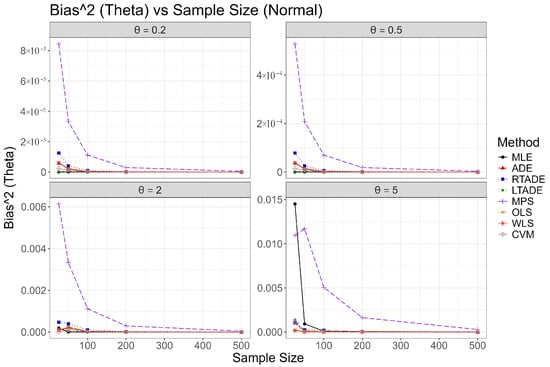
Figure 2. Plots of bias squared for the UIMB distribution across sample sizes for various $\theta$ values in the normal scenario.

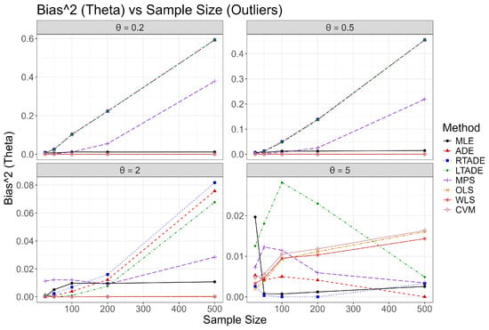
Figure 3. Plots of bias squared for the UIMB distribution across sample sizes for various $\theta$ values in the outlier scenario.

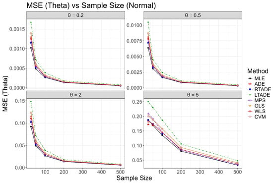
Figure 4. Plots of MSE for the UIMB distribution across sample sizes for various $\theta$ values in the normal scenario.

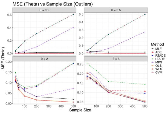
Figure 5. Plots of MSE for the UIMB distribution across sample sizes for various $\theta$ values in the outlier scenario.

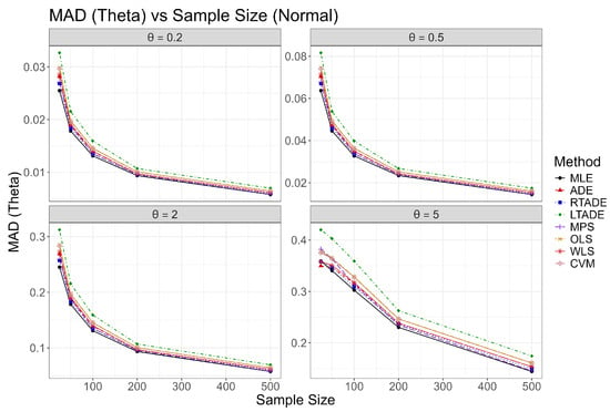
Figure 6. Plots of MAD for the UIMB distribution across sample sizes for various $\theta$ values in the normal scenario.

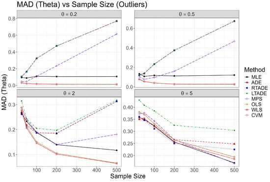
Figure 7. Plots of MAD for the UIMB distribution across sample sizes for various $\theta$ values in the outlier scenario.

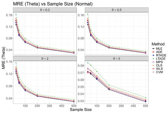
Figure 8. Plots of MRE for the UIMB distribution across sample sizes for various $\theta$ values in the normal scenario.

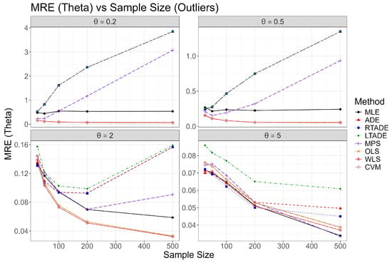
Figure 9. Plots of MRE for the UIMB distribution across sample sizes for various $\theta$ values in the outliers scenario.

These simulation analyses validate the efficacy of the proposed estimation methods, with MLE emerging as the most reliable across varying $\theta$ values and sample sizes in the normal scenario. The outliers scenario reveals that the MLE and CVM demonstrate better robustness compared to other methods.

6. Real Data Applications

This section evaluates the efficacy of the UIMB distribution in modeling three real datasets, referred to as Dataset 1, Dataset 2, and Dataset 3, to demonstrate its suitability for unit-interval data in manufacturing and mining applications. Dataset 1 consists of 50 observations with a hole diameter of 12 mm and a sheet thickness of 3.15 mm, while Dataset 2 comprises 50 observations with a hole diameter of 9 mm and a sheet thickness of 2 mm. Hole diameter readings are taken with respect to one fixed hole, selected as per a predetermined orientation, and the datasets relate to two different machines under comparison. Further details on the measurement process are provided in [24]. These datasets have also been analyzed by [25,26,27,28,29]. Dataset 3 is the Rubidium concentration dataset, which is sourced from mining engineering data [30] and normalized by dividing the original concentrations by 1000 to ensure unit-interval support. The numerical values for Dataset 1 and Dataset 2 are presented in Table 11.

Table 11. Hole Diameter Measurements for Manufacturing Datasets 1 and 2.

Dataset 1
0.04, 0.02, 0.06, 0.12, 0.14, 0.08, 0.22, 0.12, 0.08, 0.26, 0.24, 0.04, 0.14
0.16, 0.08, 0.26, 0.32, 0.28, 0.14, 0.16, 0.24, 0.22, 0.12, 0.18, 0.24, 0.32
0.16, 0.14, 0.08, 0.16, 0.24, 0.16, 0.32, 0.18, 0.24, 0.22, 0.16, 0.12, 0.24
0.06, 0.02, 0.18, 0.22, 0.14, 0.06, 0.04, 0.14, 0.26, 0.18, 0.16
Dataset 2
0.06, 0.12, 0.14, 0.04, 0.14, 0.16, 0.08, 0.26, 0.32, 0.22, 0.16, 0.12, 0.24
0.06, 0.02, 0.18, 0.22, 0.14, 0.22, 0.16, 0.12, 0.24, 0.06, 0.02, 0.18, 0.22
0.14, 0.02, 0.18, 0.22, 0.14, 0.06, 0.04, 0.14, 0.22, 0.14, 0.06, 0.04, 0.16
0.24, 0.16, 0.32, 0.18, 0.24, 0.22, 0.04, 0.14, 0.26, 0.18, 0.16

The numerical values of Dataset 3 are available in [30]. Comparisons are conducted with the Unit Maxwell–Boltzmann (UMB), Unit Topp–Leone (UTL), Unit Lindley (ULL), and Unit Log-Weighted Exponential (ULWE) distributions using maximum likelihood estimation implemented in R software [23]. The model selection criteria, integrated into the fit analysis, are defined as follows: the Akaike Information Criterion (AIC) is $\mathrm{AIC}=-2log\left(L\right)+2k$, where $log(·)$ is the log-likelihood function and k is the number of parameters; the Corrected Akaike Information Criterion (AICc) is $\mathrm{AICc}=\mathrm{AIC}+{\displaystyle \frac{2k(k+1)}{n-k-1}}$, with n as the sample size; the Bayesian Information Criterion (BIC) is $\mathrm{BIC}=-2log\left(L\right)+kln\left(n\right)$; and the Hannan-Quinn Information Criterion (HQIC) is $\mathrm{HQIC}=-2log\left(L\right)+2klog(log(n\left)\right)$. These criteria balance model fit and complexity, with lower values indicating a superior fit.

Dataset 1 exhibits a mean of 0.1632, a median of 0.1600, and a standard deviation of 0.0811, with minimal skewness and negative kurtosis, indicating a slightly right-skewed distribution with lighter tails, as given in Table 12. Fit results from Table 13 demonstrate that the UIMB distribution markedly outperforms other models, achieving the lowest values for $-2logL$ (−101.83), AIC (−99.83), AICc (−99.75), BIC (−97.92), and HQIC (−97.10), alongside Cramér–von Mises statistic (${\mathrm{W}}_{*}$) (0.14, $p=0.4313$) and Kolmogorov–Smirnov statistic (KS) (0.12, $p=0.5017$). The UMB distribution performs competitively but is less effective, while the UTL, ULL, and ULWE distributions yield significantly higher test statistics, underscoring the superior fit of the UIMB distribution. The top-left panel of Figure 10 provides visual confirmation, with the histogram of the UIMB distribution closely aligning with the burr measurements in Dataset 1.

Table 12. Descriptive statistics of Dataset 1.

n	Mean	Median	Standard Deviation	Skewness	Kurtosis	Sk./Ku.
50	0.1632	0.1600	0.0811	0.0702	−0.8711	−0.0806

Table 13. Parameter estimation and fit evaluation for Dataset 1.

Distribution	Parameters	$-2log\mathit{L}$	AIC	AICc	BIC	HQIC	${\mathbf{W}}_{*}$	${\mathbf{W}}_{*}\left(\mathit{p}\right)$	$\mathbf{KS}$	$\mathbf{KS}\left(\mathit{p}\right)$
UMB	$\theta =1.210$	−96.12	−94.12	−94.04	−92.21	−91.39	0.50	0.0403	0.22	0.015
UTL	$\theta =0.725$	−56.82	−54.82	−54.73	−52.90	−52.09	1.65	<0.01	0.36	<0.01
ULL	$\theta =1.007,\lambda ={10}^{-12}$	−63.65	−59.65	−59.40	−55.83	−54.20	1.23	<0.01	0.32	<0.01
ULWE	$\theta =0.01,\lambda =1.002$	−63.65	−59.65	−59.40	−55.83	−54.20	1.23	<0.01	0.32	<0.01
UIMB	$\theta =0.221$	−101.83	−99.83	−99.75	−97.92	−97.10	0.14	0.4313	0.12	0.5017

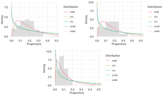
Figure 10. Fitted density histograms for Dataset 1, Dataset 2, and Dataset 3.

Dataset 2 displays a mean of 0.1520, a median of 0.1600, and a standard deviation of 0.0785, with a small skewness and negative kurtosis, reflecting a nearly symmetric distribution with lighter tails, as presented in Table 14. Fit results from Table 15 reveal that the UIMB distribution substantially outperforms other models, attaining the best $-2logL$ (−106.22), AIC (−104.22), AICc (−104.14), BIC (−102.31), and HQIC (−101.49), with ${\mathrm{W}}_{*}$ (0.20, $p=0.2594$) and KS (0.15, $p=0.1949$). The UMB distribution performs competitively but is less effective, while the UTL, ULL, and ULWE distributions exhibit significantly higher test statistics, reinforcing the superiority of the UIMB distribution. The top-right panel of Figure 10 corroborates this, with the histogram of the UIMB distribution effectively capturing the burr measurements in Dataset 2.

Table 14. Descriptive statistics of Dataset 2.

n	Mean	Median	Standard Deviation	Skewness	Kurtosis	Sk./Ku.
50	0.1520	0.1600	0.0785	0.0060	−0.7899	−0.0076

Table 15. Parameter estimation and fit evaluation for Dataset 2.

Distribution	Parameters	$-2log\mathit{L}$	AIC	AICc	BIC	HQIC	${\mathbf{W}}_{*}$	${\mathbf{W}}_{*}\left(\mathit{p}\right)$	$\mathbf{KS}$	$\mathbf{KS}\left(\mathit{p}\right)$
UMB	$\theta =1.273$	−99.52	−97.52	−97.44	−95.61	−94.80	0.59	0.0237	0.25	<0.01
UTL	$\theta =0.680$	−60.87	−58.87	−58.78	−56.95	−56.14	1.64	<0.01	0.38	<0.01
ULL	$\theta =0.960,\lambda ={10}^{-12}$	−68.26	−64.26	−64.00	−60.43	−58.80	1.22	<0.01	0.33	<0.01
ULWE	$\theta =0.01,\lambda =0.955$	−68.25	−64.25	−64.00	−60.43	−58.80	1.22	<0.01	0.33	<0.01
UIMB	$\theta =0.203$	−106.22	−104.22	−104.14	−102.31	−101.49	0.20	0.2594	0.15	0.1949

Dataset 3 exhibits a mean of 0.0886, a median of 0.0840, and a standard deviation of 0.0555, with high skewness and kurtosis, indicating a right-skewed distribution with heavy tails, as given in Table 16. Fit results from Table 17 reveal that the UIMB distribution substantially outperforms other models, attaining the best $-2logL$ (−241.27), AIC (−239.27), AICc (−239.22), BIC (−236.81), and HQIC (−236.28), with ${\mathrm{W}}_{*}$ (0.65, $p=0.0164$) and KS (0.15, $p=0.0331$). The bottom panel of Figure 10 corroborates this, with the histogram of the UIMB distribution effectively capturing the Rubidium concentrations.

Table 16. Descriptive statistics of Dataset 3.

n	Mean	Median	Standard Deviation	Skewness	Kurtosis	Sk./Ku.
86	0.0886	0.0840	0.0555	2.1946	10.4318	0.2104

Table 17. Parameter estimation and fit evaluation for Dataset 3.

Distribution	Parameters	$-2log\mathit{L}$	AIC	AICc	BIC	HQIC	${\mathbf{W}}_{*}$	${\mathbf{W}}_{*}\left(\mathit{p}\right)$	$\mathbf{KS}$	$\mathbf{KS}\left(\mathit{p}\right)$
UMB	$\theta =1.599$	−238.92	−236.92	−236.87	−234.46	−233.93	2.38	<0.01	0.33	<0.01
UTL	$\theta =0.499$	−156.09	−154.09	−154.04	−151.63	−151.10	3.85	<0.01	0.41	<0.01
ULL	$\theta =0.754,\lambda ={10}^{-11}$	−176.08	−172.08	−171.94	−167.17	−166.11	2.89	<0.01	0.35	<0.01
ULWE	$\theta =0.010,\lambda =0.750$	−176.08	−172.08	−171.94	−167.17	−166.10	2.89	<0.01	0.35	<0.01
UIMB	$\theta =0.120$	−241.27	−239.27	−239.22	−236.81	−236.28	0.65	0.0164	0.15	0.0331

The UIMB distribution demonstrates superior fitting capabilities for these datasets, leveraging its adaptable density shapes to capture the nuances of unit-interval data. Its performance surpasses that of the UMB, UTL, ULL, and ULWE distributions, as evidenced by consistently lower information criteria and superior goodness-of-fit statistics. These findings highlight the substantial potential of the UIMB distribution in reliability engineering and mining studies.

7. Conclusions

This study introduced the UIMB distribution, a novel single-parameter model tailored for unit-interval data, derived through an exponential transformation of the InvMB distribution. The UIMB distribution addresses the limitations of traditional models by offering flexible density shapes and hazard rate behaviors, including right-skewed, left-skewed, unimodal, and bathtub-shaped patterns, making it highly adaptable for applications in reliability engineering and environmental science. Its statistical properties, including moments, quantiles, survival, and hazard functions, along with stochastic ordering, entropy measures, and the moment-generating function, were thoroughly derived, demonstrating its capacity to capture complex data patterns within the ($0,1$) interval.

Simulation studies validated the robustness of various estimation methods for the scale parameter of the UIMB distribution in terms of bias, mean squared error, and mean absolute deviation across diverse sample sizes and parameter values. The inclusion of normal and outlier scenarios highlighted the adaptability of the model to skewed and contaminated data, with MLE exhibiting superior stability and resilience.

Real-data applications on two manufacturing datasets and a Rubidium concentration dataset underscored the superior fit of the UIMB distribution compared to competing models like the Unit Maxwell–Boltzmann, Unit Topp–Leone, Unit Lindley, and Unit Log-Weighted Exponential distributions. The UIMB distribution achieved the lowest values for information criteria, effectively capturing the right-skewed nature of burr measurements on iron sheets and normalized concentrations. Visual and statistical evidence confirmed its precision in modeling unit-interval phenomena.

The single-parameter design of the UIMB distribution balances computational efficiency with modeling flexibility, offering a practical tool for practitioners. Future research could explore extensions of the UIMB distribution, such as incorporating censored data models, developing Bayesian estimation approaches, or applying the model to other domains like financial ratios or biological proportions.

These findings establish the UIMB distribution as a robust and versatile addition to the statistical modeling toolkit for unit-interval data.

References

- Bayes, T. An Essay Towards Solving a Problem in the Doctrine of Chances. Philos. Trans. R. Soc. 1763, 53, 370–418. [Google Scholar] [CrossRef]
- Topp, C.W.; Leone, F.C. A Family of J-Shaped Frequency Functions. J. Am. Stat. Assoc. 1955, 50, 209–219. [Google Scholar] [CrossRef]
- Johnson, N.L.; Kotz, S.; Balakrishnan, N. Continuous Univariate Distributions, Volume 2, 2nd ed.; Wiley: Hoboken, NJ, USA, 1995. [Google Scholar]
- Mazucheli, J.; Menezes, A.F.; Dey, S. Unit-Gompertz Distribution with Applications. Statistica 2019, 79, 25–43. [Google Scholar] [CrossRef]
- Mazucheli, J.; Menezes, A.F.B.; Chakraborty, S. On the One Parameter Unit-Lindley Distribution and Its Associated Regression Model for Proportion Data. J. Appl. Stat. 2019, 46, 700–714. [Google Scholar] [CrossRef]
- Smithson, M.; Shou, Y. CDF-Quantile Distributions for Modelling RVs on the Unit Interval. Br. J. Math. Stat. Psychol. 2017, 70, 412–438. [Google Scholar] [CrossRef]
- Maxwell, J.C. On the dynamical theory of gases. Philos. Trans. R. Soc. Lond. 1867, 157, 49–88. [Google Scholar] [CrossRef]
- Bekker, A.; Roux, J. Reliability characteristics of the Maxwell distribution: A Bayes estimation study. Commun. Stat.-Theory Methods 2005, 34, 2169–2178. [Google Scholar] [CrossRef]
- Chaturvedi, A.; Rani, U. Classical and Bayesian reliability estimation of the generalized Maxwell failure distribution. J. Stat. Res. 1998, 32, 113–120. [Google Scholar]
- Tyagi, R.; Bhattacharya, S. Bayes estimation of the Maxwell’s velocity distribution function. Statistica 1989, 29, 563–567. [Google Scholar]
- Biçer, C.; Bakouch, H.S.; Biçer, H.D.; Alomair, G.; Hussain, T.; Almohisen, A. Unit Maxwell-Boltzmann Distribution and Its Application to Concentrations Pollutant Data. Axioms 2024, 13, 226. [Google Scholar] [CrossRef]
- Slezakova, K.; Castro, D.; Pereira, M.C.; Morais, S.; Delerue-Matos, C.; Alvim-Ferraz, M.C. Influence of traffic emissions on the carcinogenic polycyclic aromatic hydrocarbons in outdoor breathable particles. J. Air Waste Manag. Assoc. 2010, 60, 393–401. [Google Scholar] [CrossRef]
- Sharma, V.K.; Singh, S.K.; Singh, U. A new upside-down bathtub shaped hazard rate model for survival data analysis. Appl. Math. Comput. 2014, 239, 242–253. [Google Scholar] [CrossRef]
- Tomer, S.K.; Panwar, M.S. A Review on Inverse Maxwell Distribution with Its Statistical Properties and Applications. J. Stat. Theory Pract. 2020, 14, 33. [Google Scholar] [CrossRef]
- Singh, K.L.; Srivastava, R.S. Inverse Maxwell distribution as a survival model, genesis and parameter estimation. Res. J. Math. Stat. Sci. 2014, 2, 23–28. [Google Scholar]
- Bjerkedal, T. Acquisition of resistance in guinea pigs infected with different doses of virulent tubercle bacilli. Am. J. Hyg. 1960, 72, 130–148. [Google Scholar]
- Veriables, W.N.; Ripley, B.D. Modern Applied Statistics with S, 4th ed.; Springer: Berlin/Heidelberg, Germany, 2002. [Google Scholar] [CrossRef]
- Sharma, V.K.; Singh, S.K.; Singh, U.; Agiwal, V. The inverse Lindley distribution: A stress-strength reliability model with application to head and neck cancer data. J. Ind. Prod. Eng. 2015, 32, 163–173. [Google Scholar] [CrossRef]
- Castillo, J.S.; Goette, K.P.; Muñoz, H.A.; Gallardo, D.I.; Bourguignon, M.; Venegas, O.; Gómez, H.M. A New Generalized Gamma Generated Family of Distributions with Applications. Mathematics 2023, 11, 529. [Google Scholar] [CrossRef]
- Eaton, M.L. Group Invariance Applications in Statistics; Institute of Mathematical Statistics: Beachwood, OH, USA, 1989. [Google Scholar]
- Alzaatreh, A.; Famoye, F.; Lee, C. A new method for generating families of continuous distributions. Metron 2013, 71, 63–79. [Google Scholar] [CrossRef]
- Gradshteyn, I.S.; Ryzhik, I.M. Table of Integrals, Series, and Products, 7th ed.; Academic Press: Amsterdam, The Netherlands, 2007. [Google Scholar]
- R Core Team. R: A Language and Environment for Statistical Computing, Version 4.4.3; R Foundation for Statistical Computing: Vienna, Austria, 2025.
- Dasgupta, R. On the distribution of burr with applications. Sankhya B 2011, 73, 1–19. [Google Scholar] [CrossRef]
- Korkmaz, M.c.; Erişoglu, M. The Burr XII-geometric distribution. J. Selçuk Univ. Nat. Appl. Sci. 2014, 3, 75–87. [Google Scholar]
- Dey, S.; Mazucheli, J.; Anis, M. Estimation of reliability of multicomponent stress-strength for a kumaraswamy distribution. Commun.-Stat.-Theory Methods 2017, 46, 1560–1572. [Google Scholar] [CrossRef]
- Dey, S.; Mazucheli, J.; Nadarajah, S. Kumaraswamy distribution: Different methods of estimation. Comput. Appl. Math. 2018, 37, 2094–2111. [Google Scholar] [CrossRef]
- ZeinEldin, R.A.; Chesneau, C.; Jamal, F.; Elgarhy, M. Different estimation methods for type I half-logistic Topp-Leone distribution. Mathematics 2019, 7, 985. [Google Scholar] [CrossRef]
- Gündüz, S.; Korkmaz, M.c. A New Unit Distribution Based on the Unbounded Johnson Distribution Rule: The Unit Johnson SU Distribution. Pak. J. Stat. Oper. Res. 2020, 16, 471–490. [Google Scholar] [CrossRef]
- Reyes, J.; Rojas, M.A.; Venegas, O.; Gómez, H.W. Nakagami distribution with heavy tails and applications to mining engineering data. J. Stat. Theory Pract. 2020, 14, 55. [Google Scholar] [CrossRef]
Disclaimer/Publisher’s Note: The statements, opinions and data contained in all publications are solely those of the individual author(s) and contributor(s) and not of MDPI and/or the editor(s). MDPI and/or the editor(s) disclaim responsibility for any injury to people or property resulting from any ideas, methods, instructions or products referred to in the content. |
© 2025 by the authors. Licensee MDPI, Basel, Switzerland. This article is an open access article distributed under the terms and conditions of the Creative Commons Attribution (CC BY) license (https://creativecommons.org/licenses/by/4.0/).