Abstract
Derivative-matching approximations are constructed as power series built from functions. The method assumes knowledge of the special values of the Bell polynomials of the second kind, for which we refer to the literature. The presented ideas may have applications in numerical mathematics.
MSC:
41A58; 41A30; 41A45; 41A10; 41A20; 41A25
1. Introduction
Given a function f and a point of expansion , it is customary to say that the Taylor polynomial (TP) of degrees one, two, three, … is the best linear, quadratic, cubic, … approximation of f at . In this sense, we present several new approximations of f, such that
where, without loss of generality, we assume that the expansion is achieved at (the shift to an arbitrary point is achieved by shifting the argument). We denote the equality (1) by .
2. Power Series Built from Functions
We build as a power series of some properly chosen function g following the construction from Section 4.1.2 of [1]. We propose
The existence of a non-zero derivative at zero implies g can be inverted somewhere in the neighborhood of zero . We have
i.e., the expansion coefficients are provided by the power expansion coefficients of
This can be written in terms of Faà di Bruno’s formula, where the Bell polynomials of the second kind appear
In [1], only a few expansions were presented; in this text, we systematically review the existing formulas for special values of the Bell polynomials [2,3,4,5,6] and propose a larger number (those from [1] are also included to provide a complete list of approximations of this kind). For spatial reasons, we cannot present the derivation of these formulas here, but, as an illustration, we can mention one simple case. It is often advantageous to study derivatives of a composed function for with k fixed, because then only one term in (5) is nonzero. Let us investigate the following:
at (so ). Faà di Bruno’s formula leads to the following:
On the other hand, one has
Thus, by comparison,
the sum representing the Stirling numbers of the second kind, see expansion (9).
To keep the text brief, we organize our results as a list in which only the necessary information is summarized. We define
When needed, we extend the definition of g (or ) to zero by its limit value
and note this with ≐. The exact version of the limit (left, right, or both sides) depends on the context.
3. Expansions
The expansion, in all cases, is constructed as follows:
where we isolate the constant term so as to avoid ambiguities for (such as ) in the formulas which follow. The displayed constants directly appearing as arguments of the Bell polynomials provide the information about the derivatives of at zero for the case in question, i.e., .
3.1. Scaling
For all the functions, the scaling of the argument and of the norm that we present is possible thanks to the following formula:
Indeed, if represent the derivatives of , then , , represent the derivatives of . Thus, if one has an expansion of f based on g, one can straightforwardly, using Formula (8), write down the expansion of f in powers of
For simplicity and aesthetic reasons, we do not include this freedom in the expressions, but one should not forget that the set of expansions we actually present is significantly enlarged, since it is indexed by two real parameters: q and w.
3.2. List
- Logarithm-based expansion ()
- Exponential-based expansion ()
- Expansion with the inverse hyperbolic sine ()
- Arcus-sine-based expansion ()
- Expansion in powers of ()Notable special cases (polynomial and rational) for , . For , the TP is constructed.
- Expansion with a fraction including the square root ()
- Powers of ()
- Expansion with the Lambert function ()
- Second expansion with the Lambert function ()As readily seen from the argument of the function W (which is defined from to ∞), this approximation is valid in the right neighborhood of zero . A formal approach using and may tempt one to conclude that vanishes everywhere; however, this is not true. The argument of W is not a bijective function; thus, for , the principal branch W is not the appropriate inverse function, which implies that becomes non-trivial. An elementary analogy is , which is identically zero for but is non-constant for .
- Third expansion with the Lambert function ()As readily seen from the argument of the function W, this approximation is valid in the left neighborhood of zero (and the function is there non-trivial; see the previous case).
- Powers of sine ()where is the Kronecker delta and % is the modulo operation. This expansion has many similarities with [7] and represents a Fourier series whose standard form can be obtained by applying trigonometric power formulas to terms.
3.3. Non-Elementary g
In some situations, g is not elementary. When function is known, one can use numerical or approximation methods to obtain g in the proximity of zero.
- The formula for is shown in Equation (2.1) of [2].
- The formula for is shown in Theorem 2.7 of [2].
- The formula for is shown in Equation (3.1) of [2].
- The formula for , together with the definition of Q, is shown in Equations (5.1) and (2.3) of [3].
4. Discussion and Remarks
4.1. Plots
In Figure 1, Figure 2, Figure 3 and Figure 4, we provide plots where the four elementary functions , , and are approximated with expansions based on Equations (9)–(19), and the value and first seven derivatives are matched. For the sake of comparison, we also include the TP. The numbered subscript of approximations in the legend respects the order in which the g functions are presented in Section 3.2, and the superscript attempts to mimic the function form of g so as to remind the reader about this. The parametric expressions (13) and (16) are shown with parameters and , respectively. Some lines in the graphs are overlaid; the main reason for this is that the approximation is exact (sin(x) is exactly approximated by (19), by (13) and by (9)).
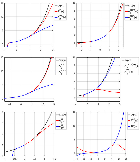
Figure 1.
The function approximated by series (6) with eight terms and with various g; from Section 3.2.
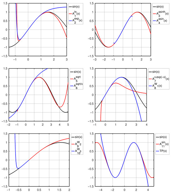
Figure 2.
The function approximated by series (6) with eight terms and with various g; from Section 3.2.
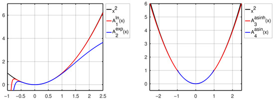
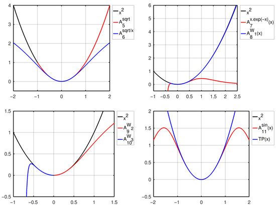
Figure 3.
The function approximated by series (6) with eight terms and with various g; from Section 3.2.
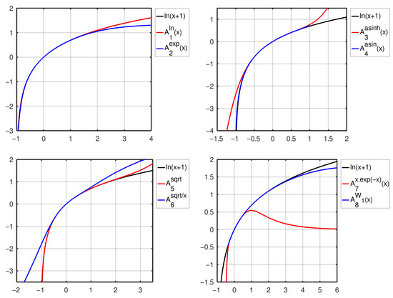
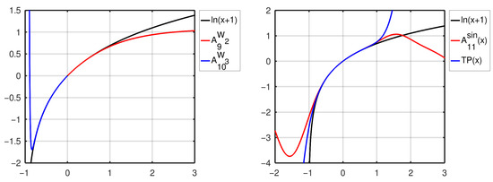
Figure 4.
The function approximated by series (6) with eight terms and with various g; from Section 3.2.
4.2. Convergence
Convergence properties can be easily addressed since the substitution, as expressed by Equation (3), does not influence the point-wise behavior. So, considering
one applies the standard convergence criteria known from the usual power series to the coefficient sequence and determines the radius of convergence R for the variable y
Then, for all , , the series converges.
The convergence to the approximated function can also be treated in the following way: for simplicity, we assume that we work on an interval containing zero, where g can be inverted. Writing an equality which includes the reminder term,
one can apply the standard criteria known from the Taylor series to see whether, in a point-wise way, the reminder vanishes with at some . If W is the set of all points, such that
then for all , such that , one has
The application of the standard criteria to may be difficult, because these, in some cases, have a complicated structure (several nested sums). The convergence criteria can be readily extended to complex analyses in a straightforward way.
4.3. Examples
The computation of the coefficients is, in some situations, possible in a closed form. Here, we present one worked example as a demonstration and list a few other cases without further justifications.
An example is the expansion of the function in powers of , as shown in Formula (15). We have
meaning that the nth derivative is equal to . One needs to compute the sum (see [8] for the proof).
This leads to
Before writing the equality sign, one needs to investigate the convergence properties. To do that, we substitute , and thus obtain
Here, the ratio test seems to be appropriate to determine the radius of the convergence R.
The convergence of the series (20) to the function is guaranteed since the latter function is analytic in the convergence domain. Indeed, it is a function composed of analytic functions and has a continuous complex derivative. The image of the interval by the function is , where As consequence, we have
For , the series diverges (because ); for , the series converges (because ) but to the wrong value (function is not bijective). To check the correctness of the expansion (20), one can use the formula , i.e., differentiate the (known) W expansion and multiply the result by −1 and by the argument.
Further expansions are possible; one can, for example, easily expand monomials , as this directly follows from (7)
Other approximations we propose (without proof, as conjecture) are as follows:
We leave the derivation to the reader.
5. Applications
The approximations listed in Section 3.2 differ a lot: one can observe various asymptotic behaviors, and some approximations are built from functions with poles, while some have branch points, etc. We consider it unlikely to find a general approach going beyond the point-vise convergence (as discussed earlier) or derivative-matching property near the expansion point, which would allow issues such as, for example, the convergence rate to be addressed. Studying different approximations separately may be a more efficient way to progress. Thus, in what follows, we propose two examples of a more detailed investigation, both based on Formula (13) with different parameters and differently scaled.
5.1. Approximating the Principal Part of Laurent Series
Let be a set of functions
If , then can be understood as a principal part of the Laurent series of some function for which the series converges everywhere except the expansion point. The following is true:
Proof.
The function is bijective, invertible . Thus, the substitution is well-defined for all
where is entire because is. Therefore, one can expand this into the Taylor series at
Now, reverting the substitution , one can obtain, for all
If the expansion equals f for all , then it has the same derivatives as f at (and everywhere else too). However, coefficients are, by construction, the unique derivative-matching coefficients for expressions of type (21); thus, . □
Several interesting comments can be made.
- Using series (21), one is able to approximate the principal part from the knowledge of its derivatives. This is different from the recipe for the Laurent series, where the coefficients are determined by the path integral around the expansion point. It is true that the derivatives contain, through analytic continuation, all information about the function and path integral values included, but we are not aware of a formula linking the Laurent series coefficients to the derivatives in a given point.
- Considering a general function and acknowledging that is a rather specific set of functions, the series (21) have a unique convergence behavior with respect to that, to our knowledge, no other derivative-matching expansion possesses—namely, they converge to the function everywhere, the non-analytic point excepted. The Taylor series reach only the singularity, which determines its convergence radius. The Neumann series of the Bessel functions, if interpreted as a derivative-matching approximation, behaves identically to the Taylor series (see [9], 16.2, “Pincherle’s theorem”). The powers of sines can be also arranged so as to fit the derivatives [7] (covered also in this text; see (19)), but this series is periodic and therefore cannot converge everywhere to f. The Padé approximants look promising; nevertheless, a ratio of two polynomials can only fit a finite number of derivatives.

Figure 5.
The function , approximated by .
5.2. Numerical Applications
The applications in numerical mathematics may result from better approximation properties than those provided by the TPs. This, however, depends on the approximated function, although some claims are evident, e.g., there are cases where an approximation proposed here converges beyond the radius of the convergence of the Taylor series. Indeed, the function , when expanded at zero, can be only approximated by the TPs at the interval . Using (9), it is exactly approximated on the whole definition interval with one term.
To be more fair, we compare the expansion in powers of , which corresponds to scaled Equation (13), with the TP inside its radius of convergence, i.e., we numerically investigate the approximation of at . We define and we obtain the following (N is the number of terms in the series; see (6)):
| N | 3 | 7 | 10 | 20 |
The first few cutoff series for both cases indicate a significant difference in the rate of convergence in favor of the expansion .
An important disadvantage for the eventual implementation of the series (9)–(19) on a computer might be the time necessary for computing from x. To speed up the evaluation of (2), Horner’s method can be used. More importantly, a couple of expansions from Section 3.2 are based on the square root, which is implemented as a basic arithmetic operation included in the instruction set of the processor in several common architectures (often labeled fsqrt; see [10] for ×86 and [11] for ARM). This means it can be evaluated very rapidly which, in combination with its possible good convergence properties, could be a reason for implementing new algorithms to compute the values of some functions (The ×86 also includes instructions for , and (fsin, f2xm1,fyl2x), which implies the approximations (19), (9) and (10) can be evaluated rapidly). Also, to speed up the numerical evaluation of a given function, the expansion coefficients need to be pre-computed and hardcoded into the body of the function as explicit numbers.
Numerical Evaluation of the Lambert W Function
To demonstrate the realistic application potential of the method, we investigate the numerical evaluation of the Lambert W function (the principal branch) on a computer in the interval . Our method of approximation is based on Formula (13) with
where e its the Euler number . We use the C/C++ language and we compare this to three other methods, namely the gsl_sf_lambert_W0 function (GSL) from the GNU Scientific Library (https://www.gnu.org/software/gsl/, accessed on 15 August 2025), the lambert_w0 method (Boost) available in the Boost C++ library (https://www.boost.org/, accessed on 15 August 2025), and method dw0c (Dwc0), presented in an academic paper [12] (all as of August 2025). For the latter, an implementation in Fortran is available, which was rewritten to C. Let us make a few comments:
- Choosing an interval may seem to be a fine-tuning method that suits us; nevertheless interval-based evaluations are very common in numerical applications and one can observe that the selected concurrency methods use this too. It is expected that one method will converge rapidly in one interval, while a different one will converge rapidly in another. This was, of course, true in our case: we conducted an expansion at .
- We do not provide a full implementation of the W function for all possible arguments; we conducted a “feasibility study”. Implementation could be based on the intervals covering the double-precision domain, with expansions for each of them, and can form part of dedicated research.
- Our system is IntelR Core™ i7-4770×8, Ubuntu 24.04.3 LTS, and the C/C++ code is compiled with a c++ (Ubuntu 13.3.0-6ubuntu2~24.04) 13.3.0 compiler. However, we carried out a relative comparison; therefore, we believe our results are system-independent.
- We provide a computer program as an addition to this text in the Supplementary Material. It contains three .cpp files: main.cpp is the executable, the alpha_20.cpp contains our method beta_20, and lambert_w.cpp contains the dw0c method of [12]. The two other methods (GSL, Boost) were linked from external libraries.
- Our approach, of course, requires a trade-off between the execution time (number of terms in the series) and the length of the interval in which full precision is achieved. If the terms up to are included, then the necessary precision is reached for ; this is our choice. We also test , where (method betaShort in alpha_20.cpp). Here, the full precision interval is small .
- We did not investigate the theoretical properties of our approach (e.g., the convergence radius) beyond providing the necessary precision.
In this setting, we repeatedly, in loops, computed the value at and for all investigated methods and measured the time. To minimize the fluctuations, we conducted computations per method. The results stand.
| Method | GSL | Boost | Dwc0 | ||
| 42.31 s | - | 144.52 s | 42.51 s | 17.04 s | |
| - | - | 0.29 | 0.99 | 2.48 | |
| 41.32 s | 15.25 s | 177.63 s | 49.12 s | 17.09 s | |
| 0.37 | - | 0.09 | 0.31 | 0.89 |
Only the numbers for a full-precision calculation are shown. It is clear that our method outperforms the two methods included in standard widespread C/C++ numerical libraries. In case of GSL, this is significant; for the Boost library, the inconclusive speed-up for is confirmed at by , although the improvement is small. The Dwc0 method surpasses ours by more than two times. However, in a small interval (too small for practical purposes, we admit), we can reduce the series enough and outcompete all studied methods. One should, however, understand how Dwc0 works: once the domain is divided into appropriate intervals, the author looks for a rational function R of a transformed argument ( for ) to describe W with with the necessary precision (double). There is no fundamental underlying approximation; it is a smart but dedicated, single-purpose construction and has some disadvantages, as follows:
- The Dwc0 is not easily scalable to a different precision. If a new precision standard is required (long double), completely new rational expressions need to be found. In our case, we just increased the number of terms.
- We believe it may sometimes be advantageous to have a justified, converging mathematical expression that has also a rapidly converging numerical implementation.
There are, presumably, two features that make Dwc0 fast: there is only one call for the sqrt(x) function (we need two) and its adjustability; all coefficients of R can be tuned. Our approximation is basically determined by derivatives and, besides the argument and the norm scaling, we have only one adjustable parameter . This is too few compared to Dwc0, but very high when compared to other standard approximations. Indeed, the choice is not arbitrary but tuned and provides much better results than the other values ( is only somewhat slower, probably because of the sqrt-s involved, although is sufficient). We believe tunable approximations, such as (13) and (16), have great application potential.
6. Summary, Conclusions, and Outlook
In this text, we presented a number of presumably new expansions built as power series constructed from functions and we addressed several related questions, such as their point-wise convergence or possible applications in numerical mathematics. In addition, we also provided a number of illustrative examples and plots. We would like to emphasize the following:
- The expansions are genuinely new; they have (in general) a different domain of convergence and a different convergence rate to the Taylor series. As a matter of fact they can be, by substitution, related to the Taylor series to investigate their properties. The latter statement does not alter the validity of the former.
- One finds, among the expansions, purely rational or polynomial expressions, namely Formula (13) for . Being based only on four basic arithmetic operations, they are well suited as practical approximations in computer- or human-performed calculations.
- Even more expansions are based on functions that are part of processor instruction sets (for common architectures) and thus can be rapidly evaluated on a computer. This leads to such expansions having realistic application potential.
Supplementary Materials
The following supporting information can be downloaded at: https://www.mdpi.com/article/10.3390/axioms14080645/s1, The supplementary material includes the full C++ source code used in this study: main.cpp (executable), alpha_20.cpp (implementation of beta_20), and lambert_w.cpp (Fukushima’s dw0c method). The code allows full reproduction of the numerical experiments and performance benchmarks.
Funding
The work was supported by VEGA grant No. 2/0084/25.
Data Availability Statement
The C/C++ source code used to evaluate the Lambert W function is provided as Supplementary Materials.
Conflicts of Interest
Author has no conflict of interest to declare.
References
- Liptaj, A. General Approach to Function Approximation. Mathematics 2024, 12, 3702. [Google Scholar] [CrossRef]
- Qi, F.; Niu, D.W.; Lim, D.; Yao, Y.H. Special values of the Bell polynomials of the second kind for some sequences and functions. J. Math. Anal. Appl. 2020, 491, 124382. [Google Scholar] [CrossRef]
- Qi, F. Taylor’s series expansions for real powers of two functions containing squares of inverse cosine function, closed-form formula for specific partial Bell polynomials, and series representations for real powers of π. Demonstr. Math. 2022, 55, 710–736. [Google Scholar] [CrossRef]
- Qi, F. Explicit formulas for partial Bell polynomials, Maclaurin’s series expansions of real powers of inverse (hyperbolic) cosine and sine, and series representations of powers of π. Preprint 2025. [Google Scholar] [CrossRef]
- Khelifa, S.; Cherruault, Y. Nouvelle identité pour les polynômes de Bell. Maghreb Math. Rev. 2000, 9, 115–123. [Google Scholar]
- Abbas, M.; Bouroubi, S. On new identities for Bell’s polynomials. Discret. Math. 2005, 293, 5–10. [Google Scholar] [CrossRef]
- Butzer, P.L.; Schmidt, K.; Stark, E.; Vogt, L. Central factorial numbers; their main properties and some applications. Numer. Funct. Anal. Optim. 1989, 10, 419–488. [Google Scholar] [CrossRef]
- Joshi, S. Discrete Calculus—Summing ∑k=1n+1k(n+1)k(-k+n+1)!. Mathematics Stack Exchange. 22 November 2015. Available online: https://math.stackexchange.com/q/1541208 (accessed on 15 August 2025).
- Watson, G.N. A Treatise on the Theory of Bessel Functions; Cambridge University Press: Cambridge, UK, 1922; Volume 3. [Google Scholar]
- Intel Corporation®. Intel 64 and IA-32 Architectures Software Developer’s Manual Combined, Volumes:1, 2A, 2B, 2C, 2D, 3A, 3B, 3C, 3D and 4. 2022. Available online: https://www.intel.com/content/www/us/en/content-details/782158/intel-64-and-ia-32-architectures-software-developer-s-manual-combined-volumes-1-2a-2b-2c-2d-3a-3b-3c-3d-and-4.html (accessed on 18 August 2025).
- Arm Limited. ArmR Compiler, version 6.6. Armasm User Guide. Arm Limited: Cambridge, UK, 2020.
- Fukushima, T. Precise and fast computation of Lambert W function by piecewise minimax rational function approximation with variable transformation. Preprints 2020. [Google Scholar] [CrossRef]


Disclaimer/Publisher’s Note: The statements, opinions and data contained in all publications are solely those of the individual author(s) and contributor(s) and not of MDPI and/or the editor(s). MDPI and/or the editor(s) disclaim responsibility for any injury to people or property resulting from any ideas, methods, instructions or products referred to in the content. |
© 2025 by the author. Licensee MDPI, Basel, Switzerland. This article is an open access article distributed under the terms and conditions of the Creative Commons Attribution (CC BY) license (https://creativecommons.org/licenses/by/4.0/).