A Study of Global Dynamics and Oscillatory Behavior of Rational-Type Nonlinear Fuzzy Difference Equations with Exponential Decay

Abstract

The concept of fuzzy modeling and fuzzy system design has opened new horizons of research in functional analysis, having a significant impact on major fields such as data science, machine learning, and so on. In this research, we use fuzzy set theory to analyze the global dynamics and oscillatory behavior of nonlinear fuzzy difference equations with exponential decay. We discuss the stability, oscillatory patterns, and convergence of solutions under different initial conditions. The exponential structure simplifies the analysis while providing a clear understanding of the system’s behavior over time. The study reveals how fuzzy parameters influence growth or decay trends, emphasizing the method’s effectiveness in handling uncertainty. Our findings advance the understanding of higher-order fuzzy difference equations and their potential applications in modeling systems with imprecise data. Using the characterization theorem, we convert a fuzzy difference equation into two crisp difference equations. The g-division technique was used to investigate local and global stability and boundedness in dynamics. We validate our theoretical results using numerical simulations.

1. Introduction

On the one hand, fuzzy difference equations provide a way to model uncertainty in discrete-time systems, and on the other, functional analysis offers tools for analyzing functions and operators. The two fields intersect when studying the behavior of solutions to fuzzy difference equations. Such solutions are described by fuzzy numbers or as a sequence of fuzzy numbers. Fuzzy numbers generalize classical real numbers to model uncertainty and imprecision and have transformed the way we represent and use data in a variety of sectors using fuzzy functional analysis [1]. It is beneficial to express uncertain or ambiguous data quantitatively, which justifies the adoption of fuzzy difference equation frameworks. Within fuzzy set theory, imperfect or unclear data can be processed effectively, enabling fuzzy difference equations to represent dynamical systems with uncertain parameters. Fuzzy difference equations find extensive utility across various domains, such as automated control mechanisms, analytical procedures, and forecasting techniques. Integrating fuzzy set theory into system modeling allows for a more realistic representation of the inherent unpredictability and intricacy in practical scenarios. Furthermore, fuzzy difference equations prove particularly suitable for analyzing nonlinear and stochastic systems. These mathematical tools show significant promise in technical fields, economic studies, and financial modeling, where sophisticated systems are prevalent [1]. The primary motivation for employing fuzzy difference equation models lies in improving the precision and reliability of system representations by accounting for real-world unpredictability and sophistication. In recent years, growing interest has emerged in both theoretical aspects and practical applications of fuzzy difference equations within applied mathematics. Taking motivation from these facts, we study the global dynamics and oscillatory behavior of nonlinear fuzzy difference equations with exponential decay in this research article. Therefore, we present the necessary review of the literature and related basic concepts in the subsequent paragraphs.

The concept of fuzzy difference equations was first introduced by Kandel and Byatt [2]. Subsequent research by Zhang et al. [3] examined the boundedness and persistence properties. A significant contribution to the field was Agarwal’s 1992 monograph [4], which provided a comprehensive treatment of difference equations and related inequalities. Kocic and Ladas [5] further advanced the field in 1993 by analyzing global behavior patterns in higher-order nonlinear difference equations. Over the years, considerable efforts have been made to analyze the qualitative behavior of nonlinear difference equations [6], particularly in the context of biological and ecological systems [7,8]. Further advancements were presented in [9], where Lyapunov functions were employed to examine the global stability of exponential difference systems. Meanwhile, Kalabušić et al. [10] focused on a Leslie–Gower-type system of rational difference equations, providing a detailed analysis of its asymptotic behavior and attractivity. Other significant contributions include the study of nonlinear rational difference equations, such as those analyzed by Ozturk et al. [11], where exponential terms and delays were shown to affect convergence and oscillatory behavior. Additionally, Touafek and Elsayed [12] considered solution structures and boundedness in rational systems, enriching the theoretical framework. Collectively, these studies underline the importance and versatility of difference equations in modeling complex real-world phenomena [13,14]. Deeba and Korvin [15] used a linearized version of the fuzzy difference equation to model $C{O}_2$ concentration in human blood. According to two mathematicians [16], the positive results of fuzzy difference equations are unique, persistent, exist, and are bounded. An equation of second order was studied by Mondal et al. [17] using the multiplier method. Based on Hukuhara’s difference as a tool for calculating fuzzy logic difference equations, Khastan [18] derived a global solution. The principle of Zadeh extension was used in [19] to study the global behavior of the fuzzy differential equation. Furthermore, the fuzzy difference equation $u_{i+1}=G+{\displaystyle \frac{u_i}{u_{i-j}}}$ was investigated in [20], where G is the non-negative fuzzy numbers and $i=(1,2)$. Stefanini [17] introduced a new approach called g-division, a generalized method for dividing fuzzy numbers. Zhang et al. [3] investigated the global dynamics of a third-order rational fuzzy difference equations using the g-partition of fuzzy numbers. Later, Khastan and Alijani [19] also examined the same model. Notably, the solutions derived using the Zadeh principle exhibit a small diameter compared to those obtained by other researchers. Recently, g-division has become a widely applied technique in fuzzy differential equations, as evidenced in [21,22]. Zhang et al. [3] studied non-zero results of finite difference equations. Ozturk et al. [11] examined a second-order crisp difference equation of exponential type. A system of exponential-type difference equations derived from Din’s work [7] revealed the existence and uniqueness of a positive equilibrium point and helped to understand the local and global behavior. Q. Zhang [23] introduced the concept of the boundedness, convergence rate, and characteristics of non-negative exponential solutions of fuzzy difference equations of order two. Furthermore, Usman et al., in [24], illustrated the concept of fuzzy difference equations of order two in a logarithmic environment. More recently, Tassaddiq et al. [25] have proposed a Ricatti-type exponential fuzzy difference equation representing the global dynamics of the fourth order. Although their study provided foundational insights into the behavior of higher-order fuzzy systems, it primarily focused on fourth-order dynamics with delayed feedback.

Understanding the dynamics of nonlinear fuzzy difference equations is crucial for analyzing systems with inherent uncertainties. Fuzzy systems have been used to represent vague and imprecise knowledge across engineering, economics, and biological modeling. Recent developments in uncertain modeling, such as the theory of uncertain numbers [26], and data-driven identification of dynamic systems through neural ODEs [27], provide a foundation for improving fuzzy system formulations. The incorporation of exponential decay into fuzzy dynamics adds an additional layer of realism, accounting for memory effects and temporal fading, which are prevalent in physical and socio-economic processes.

Clustering and classification in high-dimensional fuzzy environments have also benefited from belief-based and imprecise modeling techniques [28]. The study of collective dynamics using hypergraph-based Q-learning in multi-agent systems [29], and their relevance in public goods and decision-making scenarios, illustrates the importance of capturing nonlinear interactions in fuzzy systems. Additionally, systems that involve both information and energy transfer, such as magnetron-based power architectures [30] and grid-connected oscillation analysis [31], underscore the need for robust models to predict long-term oscillatory behavior. Techniques for identifying systemic risks in nonlinear markets [32], and polarization behaviors in complex media [33], also contribute conceptual tools that may be extended to fuzzy difference frameworks.

Taking motivation from the above review of the literature, in this article, we consider the rational case, where the fuzzy difference equation involves a ratio of exponential functions, enabling a richer dynamical structure and allowing us to explore more complex convergence and stability behavior. To simplify the structure for broader applications, we reformulate the system as a third-order exponential rational fuzzy difference equation. This reduction in order not only enhances computational efficiency but also reveals rich dynamical properties relevant to real-world fuzzy systems with fewer time-lag dependencies. Expanding this line of inquiry, we investigate the behavioral characteristics of the third-order rational exponential fuzzy difference equation. In this work, we first investigate the positive solution, then we prove that the solution must be unique and persistent. The global behavior of solutions using the g-division technique of fuzzy numbers is used. A key advantage of g-division is that it enhances the precision of fuzzy solutions by reducing the support length. This methodology enables the analysis of certain discrete-time dynamical systems taking fuzzy uncertainty into account. In this paper, we study the dynamic behavior of a nonlinear fuzzy difference equation of the form

$$u_{n+1}={\displaystyle \frac{\eta e^{-u_n}+\varphi e^{-u_{n-1}}}{\xi +u_{n-2}}},n\in \mathbb{W},$$

(1)

where $u_n$ is a sequence of fuzzy numbers, and $\eta$, $\varphi$, and $\xi$ are positive fuzzy parameters. The initial conditions are given by $u_{-2}$, $u_{-1}$, and $u_0$. Equation (1) arises as a fuzzy extension of classical nonlinear difference equations and models systems in which uncertainty or vagueness in the parameters plays a significant role.

Fuzzy difference equations have been widely investigated in recent years due to their applications in control systems, population dynamics, and economics under uncertainty. Several works such as [34,35,36] have addressed stability and boundedness properties in fuzzy discrete systems. However, most of these studies focus on either linear forms or specific bounded feedback structures. In contrast, the nonlinear and delayed structure of Equation (1) presents unique challenges and has not been extensively explored in the existing literature.

The main goal of this paper is to analyze the boundedness, stability, and equilibrium behavior of solutions to Equation (1). Our approach extends classical techniques in difference equations to the fuzzy context, providing new insights into the dynamics of such systems.

According to the plan of the paper, Section 2 reviews fundamental concepts and existing theorems. Section 3 establishes the existence and global behavior of solutions to the fuzzy difference Equation (1), supported by key characterization theorems. Section 4 validates the theoretical results through application to diverse forms of fuzzy numbers. Finally, Section 5 summarizes the conclusions and discusses potential implications.

2. Preliminaries

This section reviews several fundamental definitions and results, mostly taken from [37,38,39,40]. Throughout this work, we denote the set of real numbers by R.

Definition 1

([40]). Fuzzy numbers are functions of $t_1:S\to [0,1]$ satisfying the following conditions:

• Normality occurs when $m_1\in S$ exists such that $t_{\left(m_1\right)}=1.$
• $t_1$ is said to be a convex fuzzy number; if ∀ $0\le u_1\le 1$ and $m_1,m_2\in S$, we have $t_1(u_1{m}_1+(1-u_1)m_2)\ge min\begin{array}{c}\hfill t_1\left(m_1\right),t_2\left(m_2\right)\end{array}$.
• $t_1$ is semi-upper-continuous.
• The support of $t_1$, which would be used by $supp\left(t_1\right)=\overline{{\cup }_{\alpha \in (0,1]}{\left[t_1\right]}_{\alpha }}=\left(\overline{m_1:t_1\left(m_1\right)>o}\right)$, is compact.

The α-cut of fuzzy number $t_1$, with $0\le \alpha \le 1$, is defined by ${\left[t_1\right]}_{\alpha }=(m_1\in S:t_1\left(m_1\right)\ge \alpha )$, in particular, we have $supp\left(t_1\right)={\left[t_1\right]}_0=\left(\overline{m_1\in S|t_1\left(m_1\right)>0}\right)$.

Definition 2

([40]). Fuzzy numbers can also be represented using two functions, $v_{l,\alpha }$ and $v_{r,\alpha }$, where both functions map values from the interval $[0,1]$ to real numbers R. These functions describe the boundaries on both sides of the fuzzy numbers at different levels of certainty:

• The function $v_{l,\alpha }$ is left-continuous and exhibits a monotonically increasing behavior.
• The function $v_{r,\alpha }$ is left-continuous, monotonically decreasing, and bounded in value.
• For all $\alpha \in [0,1]$, the inequality $v_{l,\alpha }\le v_{r,\alpha }$ holds.

If a number $x_1\in R$ satisfies $(v_l\left(\alpha \right),v_r\left(\alpha \right))=(x_1,x_1)$ for all $\alpha \in [0,1]$, then the fuzzy number takes a degenerate form. The space of fuzzy numbers $R_F$ consists of all pairs $(v_l\left(\alpha \right),v_r\left(\alpha \right))$ with $0\le \alpha \le 1$, forming a convex cone that is isometrically isomorphic to a Banach space [20].

Let $\mathcal{F}\left(\mathbb{R}\right)$ denote the set of all fuzzy numbers on the real line $\mathbb{R}$. Each fuzzy number $\tilde{\mathcal{X}}\in \mathcal{F}\left(\mathbb{R}\right)$ is characterized by its family of $\alpha$-level sets $[{\ell }_{\tilde{\mathcal{X}}}\left(\alpha \right),{\rho }_{\tilde{\mathcal{X}}}\left(\alpha \right)]$ for $\alpha \in [0,1]$, where ${\ell }_{\tilde{\mathcal{X}}}\left(\alpha \right)$ and ${\rho }_{\tilde{\mathcal{X}}}\left(\alpha \right)$ denote the left and right endpoints of the interval, respectively.

Definition 3

([40]). For any $\tilde{\mathcal{X}},\tilde{\mathcal{Y}}\in \mathcal{F}\left(\mathbb{R}\right)$, the metric distance is defined as

$$d_{\infty }(\tilde{\mathcal{X}},\tilde{\mathcal{Y}})=\underset{\beta \in [0,1]}{sup}max\left(|{\ell }_{\tilde{\mathcal{X}}}\left(\beta \right)-{\ell }_{\tilde{\mathcal{Y}}}\left(\beta \right)|,|{\rho }_{\tilde{\mathcal{X}}}\left(\beta \right)-{\rho }_{\tilde{\mathcal{Y}}}\left(\beta \right)|\right)$$

Thus, the pair $(\mathcal{F}\left(\mathbb{R}\right),d_{\infty })$ constitutes a complete metric space.

Definition 4

([40]). Let $\tilde{\mathcal{P}}=({\ell }_{\mathcal{P}}\left(\gamma \right),{\rho }_{\mathcal{P}}\left(\gamma \right))$, $\tilde{\mathcal{Q}}=({\ell }_{\mathcal{Q}}\left(\gamma \right),{\rho }_{\mathcal{Q}}\left(\gamma \right))\in \mathcal{F}\left(R\right)$ for $\gamma \in [0,1]$, and let $\mu \in R$. Then,

• $\tilde{\mathcal{P}}=\tilde{\mathcal{Q}}$ iff ${\ell }_{\mathcal{P}}\left(\gamma \right)={\ell }_{\mathcal{Q}}\left(\gamma \right)$ and ${\rho }_{\mathcal{P}}\left(\gamma \right)={\rho }_{\mathcal{Q}}\left(\gamma \right)$;
• $\tilde{\mathcal{P}}+\tilde{\mathcal{Q}}=({\ell }_{\mathcal{P}}\left(\gamma \right)+{\ell }_{\mathcal{Q}}\left(\gamma \right),{\rho }_{\mathcal{P}}\left(\gamma \right)+{\rho }_{\mathcal{Q}}\left(\gamma \right))$;
• $\tilde{\mathcal{P}}-\tilde{\mathcal{Q}}=({\ell }_{\mathcal{P}}\left(\gamma \right)-{\rho }_{\mathcal{Q}}\left(\gamma \right),{\rho }_{\mathcal{P}}\left(\gamma \right)-{\ell }_{\mathcal{Q}}\left(\gamma \right))$;
• $\mu \tilde{\mathcal{P}}=\left\{\begin{array}{cc}(\mu {\ell }_{\mathcal{P}}\left(\gamma \right),\mu {\rho }_{\mathcal{P}}\left(\gamma \right)),\hfill & \mu \ge 0\hfill \\ (\mu {\rho }_{\mathcal{P}}\left(\gamma \right),\mu {\ell }_{\mathcal{P}}\left(\gamma \right)),\hfill & \mu <0\hfill \end{array}\right.$
• $\tilde{\mathcal{P}}\tilde{\mathcal{Q}}=({\zeta }_{\ell }\left(\gamma \right),{\zeta }_{\rho }\left(\gamma \right))$

where

$$\begin{array}{cc}\hfill {\zeta }_{\ell }\left(\gamma \right)& =min\{{\ell }_{\mathcal{P}}\left(\gamma \right){\ell }_{\mathcal{Q}}\left(\gamma \right),{\ell }_{\mathcal{P}}\left(\gamma \right){\rho }_{\mathcal{Q}}\left(\gamma \right),{\rho }_{\mathcal{P}}\left(\gamma \right){\ell }_{\mathcal{Q}}\left(\gamma \right),{\rho }_{\mathcal{P}}\left(\gamma \right){\rho }_{\mathcal{Q}}\left(\gamma \right)\}\hfill \\ \hfill {\zeta }_{\rho }\left(\gamma \right)& =max\{{\ell }_{\mathcal{P}}\left(\gamma \right){\ell }_{\mathcal{Q}}\left(\gamma \right),{\ell }_{\mathcal{P}}\left(\gamma \right){\rho }_{\mathcal{Q}}\left(\gamma \right),{\rho }_{\mathcal{P}}\left(\gamma \right){\ell }_{\mathcal{Q}}\left(\gamma \right),{\rho }_{\mathcal{P}}\left(\gamma \right){\rho }_{\mathcal{Q}}\left(\gamma \right)\}.\hfill \end{array}$$

Definition 5

([39]). A triangular fuzzy number $\tilde{T}=(l,m,r)$ is characterized by the following membership function:

$${\mu }_{\tilde{T}}\left(x\right)=\left\{\begin{array}{cc}0,\hfill & x\le l,\hfill \\ {\displaystyle \frac{x-l}{m-l}},\hfill & l<x\le m,\hfill \\ {\displaystyle \frac{r-x}{r-m}},\hfill & m<x\le r,\hfill \\ 0,\hfill & x>r.\hfill \end{array}\right.$$

(2)

The α-cut of $\tilde{T}$ is given by

$${\left[\tilde{T}\right]}_{\alpha }=\{x\in \mathbb{R}:{\mu }_{\tilde{T}}\left(x\right)\ge \alpha \}=[l+\alpha (m-l),r-\alpha (r-m)]=[T_{l\alpha },T_{r\alpha }],\alpha \in [0,1].$$

(3)

Each α-cut forms a closed interval. If $\mathrm{supp}\left(\tilde{T}\right)\subseteq (0,\infty )$, then $\tilde{T}$ is called a positive fuzzy number. This representation is particularly useful in applying the Stacking Theorem [40].

Theorem 1.

Let ${\left\{D_{\alpha }\right\}}_{\alpha \in [0,1]}$ be a convex family, nonempty, and the compact subset of R, satisfying

• $\overline{{\bigcup }_{\alpha >0}{D}_{\alpha }}\subseteq D_0$;
• $D_{{\alpha }_2}\subseteq D_{{\alpha }_1}$ for all ${\alpha }_1\le {\alpha }_2$;
• $D_{\alpha }={\bigcap }_{k\ge 1}{D}_{{\alpha }_k}$ when ${\alpha }_k\uparrow \alpha$ with $\alpha >0$.

Then, there exists a fuzzy number $u\in \mathcal{F}\left(R^n\right)$ such that

• ${\left[u\right]}_{\alpha }=D_{\alpha }$ for all $\alpha \in (0,1]$;
• ${\left[u\right]}_0=\overline{{\bigcup }_{0<\alpha \le 1}{D}_{\alpha }}\subseteq D_0$.

A novel division operation for fuzzy numbers, inspired by the gH-difference concept, was recently introduced by Stefanini [37].

Definition 6

([37]). For fuzzy numbers $\tilde{\mathfrak{M}},\tilde{\mathfrak{N}}\in \mathcal{F}\left(R\right)$ with α-cuts ${\left[\tilde{\mathfrak{M}}\right]}^{\alpha }=[{\mathfrak{m}}_{\prec }^{\alpha },{\mathfrak{m}}_{\succ }^{\alpha }]$ and ${\left[\tilde{\mathfrak{N}}\right]}^{\alpha }=[{\mathfrak{n}}_{\prec }^{\alpha },{\mathfrak{n}}_{\succ }^{\alpha }]$, where $0\notin {\left[\tilde{\mathfrak{N}}\right]}^{\alpha }$ for all $\alpha \in [0,1]$, the generalized division (g-division) $\tilde{\mathfrak{P}}=\tilde{\mathfrak{M}}{÷}_g\tilde{\mathfrak{N}}$ is defined by its α-cuts ${\left[\tilde{\mathfrak{P}}\right]}^{\alpha }=[{\mathfrak{p}}_{\prec }^{\alpha },{\mathfrak{p}}_{\succ }^{\alpha }]$, satisfying

1. 

The inverse operation: ${\left[\tilde{\mathfrak{P}}\right]}^{\alpha -1}=\left[{\displaystyle \frac{1}{{\mathfrak{p}}_{\succ }^{\alpha }}},{\displaystyle \frac{1}{{\mathfrak{p}}_{\prec }^{\alpha }}}\right]$.

2. 

The division condition, ${\left[\tilde{\mathfrak{P}}\right]}^{\alpha }={\left[\tilde{\mathfrak{M}}\right]}^{\alpha }{÷}_g{\left[\tilde{\mathfrak{N}}\right]}^{\alpha }$, holds if either of the following hold:

• ${\left[\tilde{\mathfrak{M}}\right]}^{\alpha }={\left[\tilde{\mathfrak{N}}\right]}^{\alpha }·{\left[\tilde{\mathfrak{P}}\right]}^{\alpha }$;
• ${\left[\tilde{\mathfrak{N}}\right]}^{\alpha }={\left[\tilde{\mathfrak{P}}\right]}^{\alpha }·{\left[\tilde{\mathfrak{M}}\right]}^{\alpha -1}$.

3. 

For $\tilde{\mathfrak{P}}$ to be a proper fuzzy number,

• ${\mathfrak{p}}_{\prec }^{\alpha }$ must be non-decreasing in α;
• ${\mathfrak{p}}_{\succ }^{\alpha }$ must be non-increasing in α;
• ${\mathfrak{p}}_{\prec }^1\le {\mathfrak{p}}_{\succ }^1$.

Let ${\mathcal{F}}^{+}\left(\mathbb{R}\right)$ denote the set of all positive fuzzy numbers on $\mathbb{R}$, i.e., fuzzy numbers whose support is a subset of $(0,\infty )$.

Remark 1.

Let $L,M\in {\mathcal{F}}^{+}\left(\mathbb{R}\right)$. If the fuzzy generalized division $N=L{÷}_{g}M$ exists and $N\in {\mathcal{F}}^{+}\left(\mathbb{R}\right)$, then according to [37], exactly one of the following cases holds:

Case I:

If $L_l^{\alpha }{M}_r^{\alpha }\le L_r^{\alpha }{M}_l^{\alpha }$ for all $\alpha \in [0,1]$, then

$$N_l^{\alpha }={\displaystyle \frac{L_l^{\alpha }}{M_l^{\alpha }}},N_r^{\alpha }={\displaystyle \frac{L_r^{\alpha }}{M_r^{\alpha }}}.$$

Case II:

If $L_l^{\alpha }{M}_r^{\alpha }\ge L_r^{\alpha }{M}_l^{\alpha }$ for all $\alpha \in [0,1]$, then

$$N_l^{\alpha }={\displaystyle \frac{L_r^{\alpha }}{M_r^{\alpha }}},N_r^{\alpha }={\displaystyle \frac{L_l^{\alpha }}{M_l^{\alpha }}}.$$

We note that the fuzzy numbers considered in [34,35] are bounded and have persistent support.

Definition 7.

A sequence $x_n$ is called a positive fuzzy solution of (1) if it satisfies the equation. The equilibrium point of (1) is positive if there exists a positive fuzzy number ${\tilde{x}}^{*}$ satisfying (1).

Definition 8.

For a sequence $\left({\tilde{x}}_n\right)$ of positive fuzzy numbers in ${\mathcal{F}}^{+}\left(R\right)$, we say ${\tilde{x}}_n\to \tilde{x}$ converges if ${lim}_{n\to \infty }D({\tilde{x}}_n,\tilde{x})=0$.

Theorem 2

([36]). (Characterization Theorem)

Let $\mathcal{F}\left(\mathbb{R}\right)$ denote the space of fuzzy numbers on $\mathbb{R}$. Consider the fuzzy difference equation

$${\tilde{y}}_{k+1}=\tilde{h}({\tilde{y}}_k,k)$$

(4)

with initial value ${\tilde{y}}_0\in \mathcal{F}\left(\mathbb{R}\right)$.

Assume the mapping $\tilde{h}:\mathcal{F}\left(\mathbb{R}\right)\times {\mathbb{Z}}_{\ge 0}\to \mathcal{F}\left(\mathbb{R}\right)$ satisfies the following:

(1) 

The α-level representation of $\tilde{h}$ is given by

$${\left[\tilde{h}({\tilde{y}}_k,k)\right]}^{\alpha }=[\underline{h}({\underline{y}}_k\left(\alpha \right),{\overline{y}}_k\left(\alpha \right),k,\alpha ),\overline{h}({\underline{y}}_k\left(\alpha \right),{\overline{y}}_k\left(\alpha \right),k,\alpha )].$$

(2) 

The functions $\underline{h}$ and $\overline{h}$ are continuous in their arguments. That is, for any $ϵ>0$, there exists $\delta >0$ such that

$$\left|\underline{h}({\underline{y}}_k\left(\alpha \right),{\overline{y}}_k\left(\alpha \right),k,\alpha )-\underline{h}({\underline{y}}_{k^{\prime }}\left(\alpha \right),{\overline{y}}_{k^{\prime }}\left(\alpha \right),k^{\prime },\alpha )\right|<ϵ$$

and

$$\left|\overline{h}({\underline{y}}_k\left(\alpha \right),{\overline{y}}_k\left(\alpha \right),k,\alpha )-\overline{h}({\underline{y}}_{k^{\prime }}\left(\alpha \right),{\overline{y}}_{k^{\prime }}\left(\alpha \right),k^{\prime },\alpha )\right|<ϵ$$

whenever

$$\parallel ({\underline{y}}_k\left(\alpha \right),{\overline{y}}_k\left(\alpha \right),k)-({\underline{y}}_{k^{\prime }}\left(\alpha \right),{\overline{y}}_{k^{\prime }}\left(\alpha \right),k^{\prime })\parallel <\delta ,\forall \alpha \in [0,1].$$

Then, the fuzzy Equation (1) is equivalent to the system of two real-valued difference equations

$${\underline{y}}_{k+1}\left(\alpha \right)=\underline{h}({\underline{y}}_k\left(\alpha \right),{\overline{y}}_k\left(\alpha \right),k,\alpha )$$

$${\overline{y}}_{k+1}\left(\alpha \right)=\overline{h}({\underline{y}}_k\left(\alpha \right),{\overline{y}}_k\left(\alpha \right),k,\alpha )$$

subject to the initial conditions

$${\underline{y}}_0\left(\alpha \right)={\underline{y}}_0\left(\alpha \right),{\overline{y}}_0\left(\alpha \right)={\overline{y}}_0\left(\alpha \right).$$

3. Uniqueness and Existence of System

We consider the fuzzy difference Equation (1). Using the characterization theorem, the fuzzy difference equation can be transformed into an equivalent system of two crisp difference equations. This decomposition serves as the foundation for our analysis within the fuzzy theoretical framework. To investigate and establish the existence and uniqueness of positive solutions, we first present the following lemma.

Let $S_1^{+}$ denote the set of all positive fuzzy numbers on $\mathbb{R}$, i.e., fuzzy numbers whose support is contained in $(0,\infty )$. Thus, $S_1^{+}={\mathcal{F}}^{+}\left(\mathbb{R}\right)$.

Lemma 1

([40]). Assume that h is the continuous operation, from $S_1^{+}\times S_1^{+}\times S_1^{+}\to S_1^{+}$, and the given $\eta ,\varphi ,$ and ξ are the fuzzy number. Then,

$$\begin{array}{c}\hfill {\left[h(\eta ,\varphi ,\xi )\right]}_{\alpha }=h({\left[\eta \right]}_{\alpha },{\left[\varphi \right]}_{\alpha },{\left[\xi \right]}_{\alpha }),\alpha \in [0,1].\end{array}$$

(5)

Theorem 3.

Consider Equation (1), where $u_n$ is a sequence of fuzzy numbers (fuzzy number), and let $\eta ,\varphi ,\xi$ be positive constants. Assume the initial conditions $u_{-2},u_{-1},u_0$ are given. Then, there exists a unique non-zero solution $u_n$ to this equation corresponding to these initial conditions.

Proof. 

The argument follows similarly to Theorem 3. Assume there exists a sequence of fuzzy numbers $u_n$ that satisfies Equation (1) under the initial conditions $u_{-2},u_{-1},u_0$. We now examine the $\alpha$-level cut for $0\le \alpha \le 1$:

$$\begin{array}{c}\hfill {\left[\eta \right]}_{\alpha }=[{\eta }_{l,\alpha },{\eta }_{r,\alpha }]and{\left[\varphi \right]}_{\alpha }=[{\varphi }_{l,\alpha },{\varphi }_{r,\alpha }]and{\left[\xi \right]}_{\alpha }=[{\xi }_{l,\alpha },{\xi }_{r,\alpha }],n=-2,-1,\dots ,\end{array}$$

From Lemma 1, it follows that now we denote the left- and right-continuous functions by $\mathrm{\Phi }$ and $\mathrm{\Psi }$:

$$\begin{array}{c}\hfill {\left[u_{n+1}\right]}_{\alpha }=[{\mathrm{\Phi }}_{n+1,\alpha },{\mathrm{\Psi }}_{n+1,\alpha }]={\left[{\displaystyle \frac{\eta e^{-u_n}+\varphi e^{-u_{n-1}}}{\xi +u_{n-2}}}\right]}_{\alpha }={\displaystyle \frac{{\left[\eta \right]}_{\alpha }{\left[e^{-u_n}\right]}_{\alpha }+{\left[\varphi \right]}_{\alpha }{\left[e^{-u_{n-1}}\right]}_{\alpha }}{{\left[\xi \right]}_{\alpha }+{\left[u_{n-2}\right]}_{\alpha }}}\\ \hfill ={\displaystyle \frac{[{\eta }_{l,\alpha }{e}^{-{\psi }_{n,\alpha }}+{\varphi }_{l,\alpha }{e}^{-{\mathrm{\Psi }}_{n-1,\alpha }},{\eta }_{r,\alpha }{e}^{-{\mathrm{\Phi }}_{n,\alpha }}+{\varphi }_{r,\alpha }{e}^{-{\mathrm{\Phi }}_{n-1,\alpha }}]}{[{\xi }_{l,\alpha }+{\mathrm{\Phi }}_{n-2,\alpha },{\xi }_{r,\alpha }+{\mathrm{\Psi }}_{n-2,\alpha }]}}\end{array}$$

According to Remark 1, we distinguish between the following two cases for further discussion:

Case I:

$$\begin{array}{c}\hfill {\left[u_{n+1}\right]}_{\alpha }=[{\mathrm{\Phi }}_{n+1,\alpha },{\mathrm{\Psi }}_{n+1,\alpha }]=\left[{\displaystyle \frac{{\eta }_{l,\alpha }{e}^{-{\mathrm{\Psi }}_{n,\alpha }}+{\varphi }_{l,\alpha }{e}^{-{\mathrm{\Psi }}_{n-1,\alpha }}}{{\xi }_{l,\alpha }+{\mathrm{\Phi }}_{n-2,\alpha }}},{\displaystyle \frac{{\eta }_{r,\alpha }{e}^{-{\mathrm{\Phi }}_n,\alpha }+{\varphi }_{r,\alpha }{e}^{-{\mathrm{\Phi }}_{n-1,\alpha }}}{{\xi }_{r,\alpha }+{\mathrm{\Psi }}_{n-2,\alpha }}}\right]\end{array}$$

(6)

Case II:

$$\begin{array}{c}\hfill {\left[u_{n+1}\right]}_{\alpha }=[{\mathrm{\Phi }}_{n+1,\alpha },{\mathrm{\Psi }}_{n+1,\alpha }]=\left[{\displaystyle \frac{{\eta }_{r,\alpha }\times e^{-{\mathrm{\Phi }}_{n,\alpha }}+{\varphi }_{r,\alpha }\times e^{-{\mathrm{\Phi }}_{n-1,\alpha }}}{{\xi }_{r,\alpha }+{\mathrm{\Psi }}_{n-2,\alpha }}},{\displaystyle \frac{{\eta }_{l,\alpha }\times e^{-{\mathrm{\Psi }}_n,\alpha }+{\varphi }_{l,\alpha }\times e^{-{\mathrm{\Psi }}_{n-1,\alpha }}}{{\xi }_{l,\alpha }+{\mathrm{\Phi }}_{n-2,\alpha }}}\right].\end{array}$$

(7)

Considering Case I, we have

$$\begin{array}{c}\hfill {\displaystyle \frac{{\eta }_{l,\alpha }\times e^{-{\mathrm{\Psi }}_{n,\alpha }}+{\varphi }_{l,\alpha }\ast e^{-{\mathrm{\Psi }}_{n-1,\alpha }}}{{\eta }_{r,\alpha }\times e^{-{\mathrm{\Phi }}_{n,\alpha }}+{\varphi }_{r,\alpha }\times e^{-{\mathrm{\Phi }}_{n-1,\alpha }}}}\le {\displaystyle \frac{{\xi }_{l,\alpha }+{\mathrm{\Phi }}_{n-2,\alpha }}{{\xi }_{r,\alpha }+{\mathrm{\Psi }}_{n-2,\alpha }}},\end{array}$$

for all $n\ge 0$ and $\alpha \in (0,1]$. Now,

$$\begin{array}{cc}\hfill {\mathrm{\Phi }}_{n+1,\alpha }& ={\displaystyle \frac{{\eta }_{l,\alpha }\times e^{-{\mathrm{\Psi }}_{n,\alpha }}+{\varphi }_{l,\alpha }\times e^{-{\mathrm{\Psi }}_{n-1,\alpha }}}{{\xi }_{l,\alpha }+{\mathrm{\Phi }}_{n-2,\alpha }}}\\ \hfill {\mathrm{\Psi }}_{n+1,\alpha }& ={\displaystyle \frac{{\eta }_{r,\alpha }\times e^{-{\mathrm{\Phi }}_{n,\alpha }}+{\varphi }_{r,\alpha }\times e^{-{\mathrm{\Phi }}_{n-1,\alpha }}}{{\xi }_{r,\alpha }+{\mathrm{\Psi }}_{n-2,\alpha }}}.\end{array}$$

(8)

It is clear that for initial condition $({\mathrm{\Phi }}_{n,\alpha },{\mathrm{\Psi }}_{n,\alpha })$, where $n\in [-2,0]$ and $0\le \alpha \le 1$, the system (8) has a unique solution of $({\mathrm{\Phi }}_{n,\alpha },{\mathrm{\Psi }}_{n,\alpha })$. On the other hand we show that $[{\mathrm{\Phi }}_{n+1,\alpha },{\mathrm{\Psi }}_{n+1,\alpha }],0\le \alpha \le 1$, where ${\mathrm{\Phi }}_{n,\alpha },{\mathrm{\Psi }}_{n,\alpha }$ is the results of system (8), $n\in [-2,0],$

$$\begin{array}{cc}\hfill {\left[u_n\right]}_{\alpha }& =[{\mathrm{\Phi }}_{n,\alpha },{\mathrm{\Psi }}_{n,\alpha }],\alpha \in [0,1],n=0,1,2,3,·\end{array}$$

(9)

Putting $n=1$, and since $\eta ,\varphi$, and $\xi$ are the positive fuzzy number and $u_n,n\in [-2,0]$, it is simple to see that $[{\mathrm{\Phi }}_{l,\alpha },{\mathrm{\Psi }}_{l,\alpha }]$ is the $\alpha$-cut of $u_1$=${\displaystyle \frac{\eta \times e^{-u_1}+\varphi \times e^{-u_{-1}}}{\xi +u_{-2}}}$, for any $\alpha \in (0,1]$. Therefore,

$$\begin{array}{ccc}\hfill [{\mathrm{\Phi }}_{1,\alpha },{\mathrm{\Psi }}_{1,\alpha }]& =\left[{\displaystyle \frac{{\eta }_{l,\alpha }\times e^{-{\mathrm{\Psi }}_{n,\alpha }}+{\varphi }_{l,\alpha }\times e^{-{\mathrm{\Psi }}_{-1,\alpha }}}{{\xi }_{l,\alpha }+{\mathrm{\Phi }}_{-2,\alpha }}},{\displaystyle \frac{{\eta }_{r,\alpha }\times e^{-{\mathrm{\Phi }}_{n,\alpha }}+{\varphi }_{r,\alpha }\times e^{-{\mathrm{\Phi }}_{-1,\alpha }}}{{\xi }_{r,\alpha }+{\mathrm{\Psi }}_{-2,\alpha }}}\right]\hfill & \hfill ={\displaystyle \frac{{\left[\eta \right]}_{\alpha }\times {\left[e^{-u_1}\right]}_{\alpha }+{\left[\varphi \right]}_{\alpha }\times {\left[e^{-u_{-1}}\right]}_{\alpha }}{{\left[\xi \right]}_{\alpha }+{\left[u_{-2}\right]}_{\alpha }}}.\end{array}$$

Proceeding inductively, suppose that $[{\mathrm{\Phi }}_{k,\alpha },{\mathrm{\Psi }}_{k,\alpha }]$ are the $\alpha$-cuts of $u_k$, i.e., ${\left[u_k\right]}_{\alpha }=[{\mathrm{\Phi }}_{k,\alpha },{\mathrm{\Psi }}_{k,\alpha }]$. It remains to prove that $[{\mathrm{\Phi }}_{k+1,\alpha },{\mathrm{\Psi }}_{k+1,\alpha }]$ represents the $\alpha$-cut of $u_{k+1}$.

$$\begin{array}{c}\hfill u_{k+1}={\displaystyle \frac{\eta \times e^{-u_k}+\varphi \ast e^{-u_{k-1}}}{\xi +u_{k-2}}}.\end{array}$$

According to Equation (8), for any $0\le \alpha \le 1$, we obtain

$$\begin{array}{c}\hfill [{\mathrm{\Phi }}_{k+1,\alpha },{\mathrm{\Psi }}_{k+1,\alpha }]=\left[{\displaystyle \frac{{\eta }_{l,\alpha }\times e^{-{\mathrm{\Psi }}_{k,\alpha }}+{\varphi }_{l,\alpha }\times e^{-{\mathrm{\Psi }}_{k-1,\alpha }}}{{\xi }_{l,\alpha }+{\mathrm{\Phi }}_{k-2,\alpha }}},{\displaystyle \frac{{\eta }_{r,\alpha }\times e^{-{\mathrm{\Phi }}_{k,\alpha }}+{\varphi }_{r,\alpha }\times e^{-{\mathrm{\Phi }}_{k-1,\alpha }}}{{\xi }_{r,\alpha }+{\mathrm{\Psi }}_{k-2,\alpha }}}\right]\end{array}$$

(10)

$$\begin{array}{c}\hfill ={\displaystyle \frac{{\left[\eta \right]}_{\alpha }\times {\left[e^{-u_k}\right]}_{\alpha }+{\left[\varphi \right]}_{\alpha }\times {\left[e^{-u_{k-1}}\right]}_{\alpha }}{{\left[\xi \right]}_{\alpha }+{\left[u_{k-2}\right]}_{\alpha }}}\end{array}$$

(11)

$$\begin{array}{c}\hfill ={\left[{\displaystyle \frac{\eta \times e^{-u_k}+\beta e^{-u_{k-1}}}{\xi +u_{k-2}}}\right]}_{\alpha }.\end{array}$$

(12)

As $[{\mathrm{\Phi }}_{k+1,\alpha },{\mathrm{\Psi }}_{k+1,\alpha }]$ represents the required $\alpha$-level set of the fuzzy number $u_{k+1}$, where

$$u_{k+1}={\displaystyle \frac{\eta \times e^{-u_k}+\varphi \times e^{-u_{k-1}}}{\xi +u_{k-2}}},$$

it follows that for all n and $0\le \alpha \le 1$, the interval $[{\mathrm{\Phi }}_{n,\alpha },{\mathrm{\Psi }}_{n,\alpha }]$ corresponds to the desired $\alpha$-level set of the fuzzy number $u_n$.

Next, we aim to establish the uniqueness of this fuzzy solution. Assume that Equation (1) admits a second solution sequence ${\overline{u}}_n$ that satisfies the same initial conditions for $n=-2,-1,0$. Then, following a similar line of reasoning as above, we have

$$\begin{array}{c}\hfill {\left[{\overline{u}}_n\right]}_{\alpha }=[{\mathrm{\Phi }}_{n,\alpha },{\mathrm{\Psi }}_{n,\alpha }],\end{array}$$

(13)

for all $0\le \alpha \le 1$ and for all $n=0,1,2,\dots$.

Hence, from Equations (9) and (10), it is evident that

$${\left[u_n\right]}_{\alpha }={\left[{\overline{u}}_n\right]}_{\alpha },\forall \alpha \in (0,1],n\in \mathbb{W}.$$

If Case II holds, the argument mirrors that of Case I, and thus the proof proceeds analogously.

To analyze the global dynamics and oscillatory behavior of nonlinear fuzzy difference equations with exponential form (1), we must first study the dynamics of their crisp counterpart. Thus, the result follows.

Following the g-division approach, we examine the two previously mentioned cases. When Case I holds, the subsequent definitions and lemmas are essential for proving the following theorems. □

Definition 9

([5]). Consider the following system of difference equations:

$$\left\{\begin{array}{c}{v}_{n+1}={\displaystyle \frac{{\eta }_1{e}^{-w_n}+{\varphi }_1{e}^{-w_{n-1}}}{{\xi }_1+v_{n-2}}}\hfill \\ w_{n+1}={\displaystyle \frac{{\eta }_2{e}^{-v_n}+{\varphi }_2{e}^{-v_{n-1}}}{{\xi }_2+w_{n-2}}}\hfill \end{array}\right.,n=0,1,2,\dots ,$$

(14)

where ${\eta }_i,{\varphi }_i,{\xi }_i$ ($i=1,2$) are positive real numbers and the initial conditions $v_i,w_i$ ($i=-2,-1,0$) are positive. A solution $\left\{(v_n,w_n)\right\}$ is called

• Positive if $v_n>0$ and $w_n>0$ for all $n\ge -2$;
• Bounded and persistent if there exist positive constants $K,L$ such that

  $$\begin{array}{c}\hfill 0<K\le v_n\le L\mathit{and}0<K\le w_n\le L\forall n\ge -2\end{array}$$

Lemma 2.

Consider the system of difference equations defined in (14). Let the initial conditions be given by $v_i,w_i$ for $i\in \{-2,-1,0\}$. Assume the following two conditions hold:

1. 

The system defined by (14) admits a positive solution that is bounded.

2. 

The system possesses a positive equilibrium point $\left(\overline{v}\right)\in (0,L_1]\times (0,L_2]$, which is locally asymptotically stable, provided that

$$\begin{array}{c}\hfill L_i={\displaystyle \frac{{\eta }_i+{\varphi }_i}{{\xi }_i}},i=1,2,\mathit{and}{\xi }_1{\xi }_2{e}^{-{\displaystyle \frac{{\xi }_1}{2}}}\ge ({\varphi }_1+{\eta }_1)({\varphi }_2+{\eta }_2),\end{array}$$

(15)

and

$$\begin{array}{c}\hfill {\displaystyle \frac{{\eta }_1{\varphi }_2}{{\xi }_1{\xi }_2}}-{\displaystyle \frac{{\varphi }_1^2}{{\xi }_2^2}}-{\displaystyle \frac{{\eta }_2+{\varphi }_2}{{\xi }_2^2}}<1.\end{array}$$

(16)

Proof. 

To proceed, (i) let $(v_n,w_n)$ be the positive result of (14), then we have

$$\begin{array}{c}\hfill v_n\le {\displaystyle \frac{{\eta }_1+{\varphi }_1}{{\xi }_1}}=L_1,w_n\le {\displaystyle \frac{{\eta }_2+{\varphi }_2}{{\xi }_2}}=L_2.\end{array}$$

(17)

Now from (14) and (17), we have

$$\begin{array}{c}\hfill v_n\ge {\displaystyle \frac{{\eta }_1\times e^{-\frac{{\eta }_2+{\varphi }_2}{{\xi }_2}}+{\varphi }_1{e}^{-\frac{{\eta }_2+{\varphi }_2}{{\xi }_2}}}{{\xi }_1+\frac{{\eta }_1+{\varphi }_1}{{\xi }_1}}}=K_1,w_n\ge {\displaystyle \frac{{\eta }_2\times e^{-\frac{{\eta }_1+{\varphi }_1}{{\xi }_1}}+{\varphi }_2{e}^{-\frac{{\eta }_1+{\varphi }_1}{{\xi }_1}}}{{\xi }_2+\frac{{\eta }_2+{\varphi }_2}{{\xi }_2}}}=K_2.\end{array}$$

(18)

From (17) and (18) we have

$$\begin{array}{c}\hfill K_1\le v_n\le L_1,K_2\le w_n\le L_2.\end{array}$$

This implies that the positive result of (14) has a bounded existence. (ii) Now, let us examine the systems

$$\begin{array}{c}\hfill v={\displaystyle \frac{{\eta }_1.e^{-w}+{\varphi }_1{e}^{-w}}{{\xi }_1+v}},w={\displaystyle \frac{{\eta }_2.e^{-v}+{\varphi }_2{e}^{-v}}{{\xi }_2+w}}\end{array}$$

(19)

This means that we are now able to write (19) as follows:

$$\begin{array}{c}\hfill v^2+{\xi }_{1}v-{\eta }_1.e^{-w}-{\varphi }_1{e}^{-w}=0and{w}^2+{\xi }_{2}v-{\eta }_2.e^{-v}-{\varphi }_2{e}^{-v}=0\end{array}$$

(20)

From the required system (20), we have

$$\begin{array}{c}\hfill v=h\left(w\right)={\displaystyle \frac{-{\xi }_1+\sqrt{{\xi }_1^2+4({\eta }_1+{\varphi }_1)e^{-w}}}{2}}\end{array}$$

and also we denote this as

$$F\left(w\right)=w^2+{\xi }_{2}w-({\eta }_2+{\varphi }_2)e^{-h\left(w\right)}.$$

(21)

Now, we obtain $F\left(w\right)<0,$ and

$$F\left(L_2\right)={\left[{\displaystyle \frac{{\eta }_2+{\varphi }_2}{{\xi }_2}}\right]}^2+{\xi }_2{\displaystyle \frac{{\eta }_2+{\varphi }_2}{{\xi }_2}}-({\eta }_2+{\varphi }_2)e^{-h\left(L_2\right)}>0.$$

(22)

Therefore, our analysis confirms the existence of at least one positive solution w satisfying $0<w\le L_2$.

By examining Equations (15) and (21), we obtain

$$\begin{array}{cc}\hfill F^{\prime }\left(w\right)& =2w+{\xi }_2-({\eta }_2+{\varphi }_2)e^{-h\left(w\right)}{h}^{\prime }\left(w\right)\hfill \\ \hfill & =2w+{\xi }_2+({\eta }_2+{\varphi }_2)e^{{\displaystyle \frac{-{\xi }_1+\sqrt{{\xi }_1^2+4({\eta }_1+{\varphi }_1)e^{-w}}}{2}}}\times {\displaystyle \frac{-({\eta }_1+{\varphi }_1)e^{-w}}{\sqrt{{\xi }_1^2+4({\eta }_1+{\varphi }_1)e^{-w}}}}\hfill \\ \hfill & \ge {\xi }_2-{\displaystyle \frac{({\varphi }_1+{\eta }_1)({\varphi }_2+{\eta }_2)}{{\xi }_1}}\times e^{{\xi }_1/2}>0.\hfill \end{array}$$

Therefore, the equation $F\left(w\right)=0$ admits a unique positive equilibrium point $\overline{w}\in (0,L_2]$. Similarly, there exists a unique positive equilibrium $\overline{v}\in (0,L_1]$.

Moreover, the Jacobian matrix $J_{\overline{v},\overline{w}}$ of system (1), evaluated at $(\overline{v},\overline{w})$, is given by

$$J_{\overline{v},\overline{w}}=\left[\begin{array}{cccccc}0& 0& D_1& E_1& E_2& 0\\ 1& 0& 0& 0& 0& 0\\ 0& 1& 0& 0& 0& 0\\ E_3& E_4& 0& 0& 0& D_2\\ 0& 0& 0& 1& 0& 0\\ 0& 0& 0& 0& 1& 0\end{array}\right],$$

where $D_1=-{\displaystyle \frac{{\eta }_1{e}^{-\overline{w}}+{\varphi }_1{e}^{-\overline{w}}}{{\left({\xi }_1+\overline{v}\right)}^2}}$, $E_1=-{\displaystyle \frac{{\eta }_1{e}^{-\overline{w}}}{{\xi }_1+\overline{v}}}$, $E_2=-{\displaystyle \frac{{\varphi }_1{e}^{-\overline{w}}}{{\xi }_1+\overline{v}}}$, $E_3=-{\displaystyle \frac{{\eta }_2{e}^{-\overline{v}}}{{\varphi }_2+\overline{w}}}$, $D_2=-{\displaystyle \frac{{\eta }_2.e^{-\overline{v}}+{\varphi }_2{e}^{-\overline{v}}}{{\left({\xi }_2+\overline{w}\right)}^2}}$, $E_4=-{\displaystyle \frac{{\varphi }_2{e}^{-\overline{w}}}{{\xi }_2+\overline{v}}}$.

We now derive the characteristic equation of the Jacobian matrix $J_{(\overline{v},\overline{w})}$ evaluated at the equilibrium point $(\overline{v},\overline{w})$, which is given by

$$\begin{array}{c}\hfill {\lambda }^6-{\lambda }^4(D_1+E_1{E}_2)-{\lambda }^3(E_1{E}_4+E_2^2+D_2)-{\lambda }^2\left(E_2{E}_4\right)-\lambda (D_1{D}_2+E_1{D}_2)=0.\end{array}$$

(23)

To find the characteristic equation we take absolute values of ${\lambda }^3$, i.e,

$$\begin{array}{c}\hfill |E_1{E}_4+E_2^2+D_2|=|(-{\displaystyle \frac{{\eta }_1{e}^{-\overline{w}}}{{\xi }_1+\overline{v}}})(-{\displaystyle \frac{{\varphi }_2{e}^{-\overline{w}}}{{\xi }_2+\overline{v}}})+{(-{\displaystyle \frac{{\varphi }_1{e}^{-\overline{w}}}{{\xi }_1+\overline{v}}})}^2+(-{\displaystyle \frac{{\eta }_2.e^{-\overline{v}}+{\varphi }_2{e}^{-\overline{v}}}{{\left({\xi }_2+\overline{w}\right)}^2}})|<1\end{array}$$

By Remark 1 of [5], we conclude that $(\overline{v},\overline{w})$ is asymptotically stable. □

Lemma 3.

The equilibrium point $(\overline{\vartheta },\overline{\xi })=(\overline{\varrho },\overline{\varsigma })$ of (14) is said to be globally stable if

$${\zeta }_1{e}^{-{\mathrm{\Lambda }}_2}+{\psi }_1{e}^{-{\mathrm{\Lambda }}_2}<\overline{\varrho }({\chi }_1+{\mathrm{\Lambda }}_1),{\zeta }_2{e}^{-{\mathrm{\Lambda }}_1}+{\psi }_2{e}^{-{\mathrm{\Lambda }}_1}<\overline{\varsigma }({\chi }_2+{\mathrm{\Lambda }}_2)$$

(24)

Proof. 

${\mathrm{\Delta }}_t=\overline{\varrho }\left(-1+{\displaystyle \frac{{\vartheta }_t}{\overline{\varrho }}}-ln{\displaystyle \frac{{\vartheta }_t}{\overline{\varrho }}}\right)+\overline{\varsigma }\left(-1+{\displaystyle \frac{{\xi }_t}{\overline{\varsigma }}}-ln{\displaystyle \frac{{\xi }_t}{\overline{\varsigma }}}\right)$.

Since $-1+\vartheta -ln\vartheta \ge 0$ for all $\vartheta >0$, then we have ${\mathrm{\Delta }}_t\ge 0$. Moreover, we conclude that

$$-ln{\displaystyle \frac{{\vartheta }_{t+1}}{{\vartheta }_t}}=ln{\displaystyle \frac{{\vartheta }_t}{{\vartheta }_{t+1}}}=ln\left(1-\left(1-{\displaystyle \frac{{\vartheta }_t}{{\vartheta }_{t+1}}}\right)\right)\le -\left(1-{\displaystyle \frac{{\vartheta }_t}{{\vartheta }_{t+1}}}\right)\le -{\displaystyle \frac{{\vartheta }_{t+1}-{\vartheta }_t}{{\vartheta }_{t+1}}}.$$

(25)

$$-ln{\displaystyle \frac{{\xi }_{t+1}}{{\xi }_t}}=ln{\displaystyle \frac{{\xi }_t}{{\xi }_{t+1}}}=ln\left(1-\left(1-{\displaystyle \frac{{\xi }_t}{{\xi }_{t+1}}}\right)\right)\le -\left(1-{\displaystyle \frac{{\xi }_t}{{\xi }_{t+1}}}\right)\le -{\displaystyle \frac{{\xi }_{t+1}-{\xi }_t}{{\xi }_{t+1}}}.$$

(26)

Now, we take the difference ${\mathrm{\Delta }}_{t+1}-{\mathrm{\Delta }}_t$:

$$\begin{array}{cc}\hfill {\mathrm{\Delta }}_{t+1}-{\mathrm{\Delta }}_t& =\overline{\varrho }\left(-1+{\displaystyle \frac{{\vartheta }_{t+1}}{\overline{\varrho }}}-ln{\displaystyle \frac{{\vartheta }_{t+1}}{\overline{\varrho }}}\right)+\overline{\varsigma }\left(-1+{\displaystyle \frac{{\xi }_{t+1}}{\overline{\varsigma }}}-ln{\displaystyle \frac{{\xi }_{t+1}}{\overline{\varsigma }}}\right)\hfill \\ \hfill & -\overline{\varrho }\left(-1+{\displaystyle \frac{{\vartheta }_t}{\overline{\varrho }}}-ln{\displaystyle \frac{{\vartheta }_t}{\overline{\varrho }}}\right)-\overline{\varsigma }\left(-1+{\displaystyle \frac{{\xi }_t}{\overline{\varsigma }}}-ln{\displaystyle \frac{{\xi }_t}{\overline{\varsigma }}}\right)\hfill \\ \hfill & =({\vartheta }_{t+1}-{\vartheta }_t)+({\xi }_{t+1}-{\xi }_t)-\overline{\varrho }ln{\displaystyle \frac{{\vartheta }_{t+1}}{\overline{\varrho }}}-\overline{\varsigma }ln{\displaystyle \frac{{\xi }_{t+1}}{\overline{\varsigma }}}\hfill \\ \hfill & \le ({\vartheta }_{t+1}-{\vartheta }_t)+({\xi }_{t+1}-{\xi }_t)-\overline{\varrho }{\displaystyle \frac{{\vartheta }_{t+1}-{\vartheta }_t}{{\vartheta }_{t+1}}}-\overline{\varsigma }{\displaystyle \frac{{\xi }_{t+1}-{\xi }_t}{{\xi }_{t+1}}}\hfill \\ \hfill & =({\vartheta }_{t+1}-{\vartheta }_t)\left(1-{\displaystyle \frac{\overline{\varrho }}{{\vartheta }_{t+1}}}\right)+({\xi }_{t+1}-{\xi }_t)\left(1-{\displaystyle \frac{\overline{\varsigma }}{{\xi }_{t+1}}}\right)\hfill \end{array}$$

$$=({\vartheta }_{t+1}-{\vartheta }_t)\left(1-{\displaystyle \frac{\overline{\varrho }({\chi }_1+{\vartheta }_{t-2})}{{\zeta }_1{e}^{-{\xi }_t}+{\psi }_1{e}^{-{\xi }_{t-1}}}}\right)+({\xi }_{t+1}-{\xi }_t)\left(1-{\displaystyle \frac{\overline{\varsigma }({\chi }_2+{\xi }_{t-2})}{{\zeta }_2{e}^{-{\vartheta }_t}+{\psi }_2{e}^{-{\vartheta }_{t-1}}}}\right).$$

(27)

Under condition (3), for any $\xi \ge 0$, we have

$$\begin{array}{cc}\hfill {\mathrm{\Delta }}_{t+1}-{\mathrm{\Delta }}_t& \le (M_1-{\mathrm{\Lambda }}_1)\left({\displaystyle \frac{{\zeta }_1{e}^{-{\mathrm{\Lambda }}_2}+{\psi }_1{e}^{-{\mathrm{\Lambda }}_2}-\overline{\varrho }({\chi }_1+{\mathrm{\Lambda }}_1)}{{\zeta }_1{e}^{-{\mathrm{\Lambda }}_2}+{\psi }_1{e}^{-{\mathrm{\Lambda }}_2}}}\right)\hfill \\ \hfill & \le 0\hfill \end{array}$$

This implies that ${lim}_{t\to \infty }{\mathrm{\Delta }}_t\ge 0$ and ${lim}_{t\to \infty }({\mathrm{\Delta }}_{t-1}-{\mathrm{\Delta }}_t)=0$. Thus we conclude that ${lim}_{t\to \infty }({\vartheta }_t,{\xi }_t)=(\overline{\varrho },\overline{\varsigma })$.

When we used condition (ii) of Lemma 2, we proved that $(\overline{\varrho },\overline{\varsigma })$ is globally stable. □

Theorem 4.

Consider the fuzzy difference equation of (1):

$$\begin{array}{c}\hfill {\displaystyle \frac{{\kappa }_{l,\alpha }{e}^{-{\mathrm{\Gamma }}_{n,\alpha }}+{\omega }_{l,\alpha }{e}^{-{\mathrm{\Gamma }}_{n-1,\alpha }}}{{\kappa }_{r,\alpha }{e}^{-{\mathrm{\Lambda }}_{n,\alpha }}+{\omega }_{r,\alpha }{e}^{-{\mathrm{\Lambda }}_{n-1,\alpha }}}}\le {\displaystyle \frac{{\sigma }_{l,\alpha }+{\mathrm{\Lambda }}_{n-2,\alpha }}{{\sigma }_{r,\alpha }+{\mathrm{\Gamma }}_{n-2,\alpha }}},\forall n\in \mathbb{W}\mathit{and}0<\alpha \le 1.\end{array}$$

(28)

Then, two conditions hold:

(i) 

Every positive solution $v_n$ of (1) exists and is bounded.

(ii) 

Every positive solution $v_n$ of (1) converges to a unique equilibrium point v as $n\to \infty$, and for all $0<\alpha \le 1.$

$$\begin{array}{c}\hfill {\sigma }_{l,\alpha }{\sigma }_{r,\alpha }{e}^{-{\displaystyle \frac{{\sigma }_{l,\alpha }}{2}}}>{\omega }_{l,\alpha }{\omega }_{r,\alpha },\end{array}$$

(29)

and

$$\begin{array}{c}\hfill {\displaystyle \frac{{\kappa }_{l,\alpha }+{\omega }_{l,\alpha }}{{\sigma }_{l,\alpha }^2}}+{\displaystyle \frac{{\kappa }_{r,\alpha }+{\omega }_{r,\alpha }}{{\sigma }_{r,\alpha }^2}}+{\displaystyle \frac{{\omega }_{l,\alpha }{\omega }_{r,\alpha }}{{\sigma }_{l,\alpha }{\sigma }_{r,\alpha }}}+{\displaystyle \frac{{\kappa }_{l,\alpha }+{\omega }_{l,\alpha }}{{\sigma }_{l,\alpha }}}{\displaystyle \frac{{\kappa }_{r,\alpha }+{\omega }_{r,\alpha }}{{\sigma }_{r,\alpha }}}<1.\end{array}$$

(30)

Proof. 

(i) Since $\kappa ,\omega ,\sigma ,v_{-2},v_{-1},v_0\in R_{\mathcal{F}}^{+}$, there exist positive numbers $a_{\kappa },b_{\kappa },a_{\omega },b_{\omega },a_{\sigma },b_{\sigma },a_{-2},b_{-2},a_{-1},b_{-1},a_0,b_0$ such that

$$\begin{array}{c}\hfill [{\kappa }_{l,\alpha },{\kappa }_{r,\alpha }]\subseteq [a_{\kappa },b_{\kappa }],[{\omega }_{l,\alpha },{\omega }_{r,\alpha }]\subseteq [a_{\omega },b_{\omega }],[{\sigma }_{l,\alpha },{\sigma }_{r,\alpha }]\subseteq [a_{\sigma },b_{\sigma }]\end{array}$$

$$\begin{array}{c}\hfill [{\mathrm{\Lambda }}_{-2,\alpha },{\mathrm{\Gamma }}_{-2,\alpha }]\subseteq [a_{-2},b_{-2}],[{\mathrm{\Lambda }}_{-1,\alpha },{\mathrm{\Gamma }}_{-1,\alpha }]\subseteq [a_{-1},b_{-1}],[{\mathrm{\Lambda }}_{0,\alpha },{\mathrm{\Gamma }}_{0,\alpha }]\subseteq [a_0,b_0]\end{array}$$

(31)

Let $v_n$ be a positive solution of (1). Using (28), (31), and Lemma 2, we get

$${\mathrm{\Lambda }}_{n,\alpha }\ge {\displaystyle \frac{{\kappa }_{l,\alpha }{e}^{-\frac{b_{\kappa }+b_{\omega }}{a_{\sigma }}}+{\omega }_{l,\alpha }{e}^{-\frac{b_{\kappa }+b_{\omega }}{a_{\sigma }}}}{{\sigma }_{l,\alpha }+\frac{{\kappa }_{l,\alpha }+{\omega }_{l,\alpha }}{{\sigma }_{l,\alpha }}}}\ge {\displaystyle \frac{a_{\kappa }{e}^{-\frac{b_{\kappa }+b_{\omega }}{a_{\sigma }}}+a_{\omega }{e}^{-\frac{b_{\kappa }+b_{\omega }}{a_{\sigma }}}}{b_{\sigma }+\frac{b_{\kappa }+b_{\omega }}{a_{\sigma }}}}=\rho .$$

$$\begin{array}{c}\hfill {\mathrm{\Gamma }}_{n,\alpha }\le {\displaystyle \frac{{\kappa }_{r,\alpha }+{\omega }_{r,\alpha }}{{\sigma }_{r,\alpha }}}\le {\displaystyle \frac{b_{\kappa }+b_{\omega }}{a_{\sigma }}}=\tau .\end{array}$$

(32)

This shows that $[{\mathrm{\Lambda }}_{n,\alpha },{\mathrm{\Gamma }}_{n,\alpha }]\subseteq [\rho ,\tau ]$ is bounded and persistent.

For (ii), consider

$$\begin{array}{c}\hfill {\mathrm{\Lambda }}_{\alpha }={\displaystyle \frac{{\kappa }_{l,\alpha }{e}^{-{\mathrm{\Gamma }}_{\alpha }}+{\omega }_{l,\alpha }{e}^{-{\mathrm{\Gamma }}_{\alpha }}}{{\sigma }_{l,\alpha }+{\mathrm{\Lambda }}_{\alpha }}},{\mathrm{\Gamma }}_{\alpha }={\displaystyle \frac{{\kappa }_{r,\alpha }{e}^{-{\mathrm{\Lambda }}_{\alpha }}+{\omega }_{r,\alpha }{e}^{-{\mathrm{\Lambda }}_{\alpha }}}{{\sigma }_{r,\alpha }+{\mathrm{\Gamma }}_{\alpha }}},\alpha \in (0,1].\end{array}$$

(33)

From this,

$${\displaystyle \frac{{\kappa }_{l,\alpha }{e}^{-\frac{{\kappa }_{r,\alpha }+{\omega }_{r,\alpha }}{{\sigma }_{r,\alpha }}}+{\omega }_{l,\alpha }{e}^{-\frac{{\kappa }_{r,\alpha }+{\omega }_{r,\alpha }}{{\sigma }_{r,\alpha }}}}{{\sigma }_{l,\alpha }+\frac{{\kappa }_{l,\alpha }+{\omega }_{l,\alpha }}{{\sigma }_{l,\alpha }}}}\le {\mathrm{\Lambda }}_{\alpha }\le {\displaystyle \frac{{\kappa }_{l,\alpha }+{\omega }_{l,\alpha }}{{\sigma }_{l,\alpha }}}.$$

(34)

Let ${\left[v_n\right]}_{\alpha }=[{\mathrm{\Lambda }}_{n,\alpha },{\mathrm{\Gamma }}_{n,\alpha }]$. From (28),

$$\begin{array}{cc}\hfill {\mathrm{\Lambda }}_{n+1,\alpha }& ={\displaystyle \frac{{\kappa }_{l,\alpha }{e}^{-{\mathrm{\Gamma }}_{n,\alpha }}+{\omega }_{l,\alpha }{e}^{-{\mathrm{\Gamma }}_{n-1,\alpha }}}{{\sigma }_{l,\alpha }+{\mathrm{\Lambda }}_{n-2,\alpha }}}\hfill \end{array}$$

(35)

$$\begin{array}{cc}\hfill {\mathrm{\Gamma }}_{n+1,\alpha }& ={\displaystyle \frac{{\kappa }_{r,\alpha }{e}^{-{\mathrm{\Lambda }}_{n,\alpha }}+{\omega }_{r,\alpha }{e}^{-{\mathrm{\Lambda }}_{n-1,\alpha }}}{{\sigma }_{r,\alpha }+{\mathrm{\Gamma }}_{n-2,\alpha }}}.\hfill \end{array}$$

(36)

Based on Conditions (29) and (30), and by applying Lemmas 2 and 3, it follows that Equation (35) possesses a unique equilibrium point $({\mathrm{\Lambda }}_{\alpha },{\mathrm{\Gamma }}_{\alpha })$ given by

$$\underset{n\to \infty }{lim}{\mathrm{\Lambda }}_{n,\alpha }={\mathrm{\Lambda }}_{\alpha },\underset{n\to \infty }{lim}{\mathrm{\Gamma }}_{n,\alpha }={\mathrm{\Gamma }}_{\alpha }$$

(37)

From (32) and (34), for $0<{\alpha }_1<{\alpha }_2<1$,

$$0<{\mathrm{\Lambda }}_{{\alpha }_1}\le {\mathrm{\Lambda }}_{{\alpha }_2}\le {\mathrm{\Gamma }}_{{\alpha }_2}\le {\mathrm{\Gamma }}_{{\alpha }_1}<\infty .$$

(38)

The left-continuity of the coefficients implies left-continuity of ${\mathrm{\Lambda }}_{\alpha },{\mathrm{\Gamma }}_{\alpha }$. Moreover,

$$\begin{array}{c}\hfill c={\displaystyle \frac{a_{\kappa }{e}^{-\frac{b_{\kappa }+b_{\omega }}{a_{\sigma }}}+a_{\omega }{e}^{-\frac{b_{\kappa }+b_{\omega }}{a_{\sigma }}}}{b_{\sigma }+\frac{b_{\kappa }+b_{\omega }}{a_{\sigma }}}}\le {\mathrm{\Lambda }}_{\alpha }\le {\mathrm{\Gamma }}_{\alpha }\le {\displaystyle \frac{b_{\kappa }+b_{\omega }}{a_{\sigma }}}=d.\end{array}$$

(39)

Thus ${\cup }_{\alpha \in (0,1]}[{\mathrm{\Lambda }}_{\alpha },{\mathrm{\Gamma }}_{\alpha }]\subset [c,d]$ is compact. There exists $v\in R_{\mathcal{F}}$ satisfying

$$\begin{array}{c}\hfill v={\displaystyle \frac{\kappa e^{-v}+\omega e^{-v}}{\sigma +v}},{\left[v\right]}_{\alpha }=[{\mathrm{\Lambda }}_{\alpha },{\mathrm{\Gamma }}_{\alpha }],\alpha \in (0,1].\end{array}$$

(40)

Uniqueness follows similarly. Finally,

$$\begin{array}{c}\hfill \underset{n\to \infty }{lim}D(v_n,v)=\underset{n\to \infty }{lim}\underset{\alpha \in (0,1]}{sup}max\left\{\right|{\mathrm{\Lambda }}_{n,\alpha }-{\mathrm{\Lambda }}_{\alpha }|,|{\mathrm{\Gamma }}_{n,\alpha }-{\mathrm{\Gamma }}_{\alpha }\left|\right\}=0,\end{array}$$

proving global convergence to the unique equilibrium point v. □

Lemma 4.

Consider the following system of difference equations:

$$v_{n+1}={\displaystyle \frac{{\eta }_2{e}^{-v_n}+{\varphi }_2{e}^{-v_{n-1}}}{{\xi }_2+w_{n-2}}},w_{n+1}={\displaystyle \frac{{\eta }_1{e}^{-w_n}+{\varphi }_1{e}^{w_{n-1}}}{{\xi }_1+v_{n-2}}},n=0,1,2,\dots ,\forall {\eta }_i,{\varphi }_i,{\xi }_i,\in (0,+\infty ),$$

(41)

with $i=1,2$ the initial condition and $v_{-2},w_{-2},v_{-1},w_{-1},v_0,w_0\in (0,+\infty )$. Then, the following two conditions hold:

(i) 

All trajectories of (41) remain bounded and the system is persistent.

(ii) 

The systems of (41) must have a unique positive equilibrium point.

$$\begin{array}{c}\hfill (\overline{v},\overline{w})\in [P_1={\displaystyle \frac{{\eta }_2{e}^{-\frac{{\alpha }_2+{\beta }_2}{a_2}}+{\varphi }_2{e}^{-\frac{{\eta }_2+{\varphi }_2}{{\xi }_2}}}{{\xi }_2+\frac{{\eta }_1+{\varphi }_1}{{\xi }_1}}},Q_1={\displaystyle \frac{{\eta }_2+{\varphi }_2}{{\xi }_2}}]\times [P_2={\displaystyle \frac{{\eta }_1{e}^{-\frac{{\eta }_1+{\varphi }_1}{{\xi }_1}}+{\varphi }_1{e}^{-\frac{{\eta }_1+{\varphi }_1}{{\xi }_1}}}{{\xi }_1+\frac{{\eta }_2+{\varphi }_2}{{\xi }_2}}},Q_2={\displaystyle \frac{{\eta }_1+{\varphi }_1}{{\xi }_1}}]\end{array}$$

if

$$\begin{array}{c}\hfill ((Q_2+1){\varphi }_1{e}^{-P_2}+{\eta }_1{e}^{-P_2})((\mathrm{\Gamma }-1){\varphi }_2{e}^{\mathrm{\Gamma }}+{\eta }_2{e}^{\mathrm{\Gamma }})<P_2^2{\mathrm{\Gamma }}^2\end{array}$$

(42)

and

$$\begin{array}{c}\hfill ((Q_1+1){\varphi }_2{e}^{-P_1}+{\eta }_2{e}^{-P_1})((\gamma -1){\varphi }_1{e}^{\gamma }+{\eta }_1{e}^{\gamma })<P_1^2{\gamma }^2,\end{array}$$

(43)

where

$$\begin{array}{c}\hfill \mathrm{\Gamma }=-({\displaystyle \frac{{\eta }_1{e}^{-Q_2}+{\varphi }_1{e}^{-Q_2}}{Q_2}}-{\xi }_1),\gamma =-({\displaystyle \frac{{\eta }_2{e}^{-Q_1}+{\varphi }_2{e}^{-Q_1}}{Q_1}}-{\xi }_2)\end{array}$$

Proof. 

(i) From (41) it is clear that

$$\begin{array}{c}\hfill v_n\le {\displaystyle \frac{{\eta }_2+{\varphi }_2}{{\xi }_2}}=Q_1,w_n\le {\displaystyle \frac{{\eta }_1+{\varphi }_1}{{\xi }_1}}=Q_2.\end{array}$$

(44)

By (41) and (44), we have

$$v_n\ge {\displaystyle \frac{{\eta }_2{e}^{-\frac{{\eta }_2+{\varphi }_2}{{\xi }_2}}+{\varphi }_2{e}^{-\frac{{\eta }_2+{\varphi }_2}{{\xi }_2}}}{{\xi }_2+\frac{{\eta }_1+{\varphi }_1}{{\xi }_1}}}=P_1,w_n\ge {\displaystyle \frac{{\eta }_1{e}^{-\frac{{\eta }_1+{\varphi }_1}{{\xi }_1}}+{\varphi }_1{e}^{-\frac{{\eta }_1+{\varphi }_1}{{\xi }_1}}}{{\xi }_1+\frac{{\eta }_2+{\varphi }_2}{{\xi }_2}}}=P_2$$

(45)

Now, from Equations (44) and (45) we see that Equation (10) is persistent and bounded, i.e.,

$$\begin{array}{c}\hfill P_1\le v_n\le Q_1,and{P}_2\le w_n\le Q_2,n\ge 1.\end{array}$$

(ii) implies that we consider

$$\begin{array}{c}\hfill v={\displaystyle \frac{{\eta }_2{e}^{-v}+{\varphi }_2{e}^{-v}}{{\xi }_2+w}},w={\displaystyle \frac{{\eta }_1{e}^{-w}+{\varphi }_1{e}^w}{{\xi }_1+v}}\end{array}$$

(46)

Equation (46) can also be written as

$$w={\displaystyle \frac{{\eta }_2{e}^{-v}+{\varphi }_2{e}^{-v}-{\xi }_{2}v}{v}},v={\displaystyle \frac{{\eta }_1{e}^{-w}+{\varphi }_1{e}^{-w}-{\xi }_{1}w}{w}}.$$

(47)

Now, from (47) we have

$$\begin{array}{c}\hfill F\left(w\right)={\displaystyle \frac{{\eta }_2{e}^{-g\left(w\right)}+{\varphi }_2{e}^{-g\left(w\right)}}{g\left(w\right)}}-{\xi }_2-w,\end{array}$$

(48)

where

$$v=g\left(w\right)={\displaystyle \frac{{\eta }_1{e}^{-w}+{\varphi }_1{e}^{-w}-{\xi }_{1}w}{w}},w\in [P_2={\displaystyle \frac{{\eta }_1{e}^{-\frac{{\eta }_1+{\varphi }_1}{{\xi }_1}}+{\varphi }_1{e}^{-\frac{{\eta }_1+{\varphi }_1}{{\xi }_1}}}{{\xi }_1+\frac{{\eta }_2+{\varphi }_2}{{\xi }_2}}},Q_2={\displaystyle \frac{{\eta }_1+{\varphi }_1}{{\xi }_1}}].$$

(49)

We have

$$\begin{array}{c}\hfill F\left(w\right):[P_2={\displaystyle \frac{{\eta }_1{e}^{-\frac{{\eta }_1+{\varphi }_1}{{\xi }_1}}+{\varphi }_1{e}^{-\frac{{\eta }_1+{\varphi }_1}{{\xi }_1}}}{{\xi }_1+\frac{{\eta }_2+{\varphi }_2}{{\xi }_2}}},Q_2={\displaystyle \frac{{\eta }_1+{\varphi }_1}{{\xi }_1}}]\to \\ \hfill [P_2={\displaystyle \frac{{\eta }_1{e}^{-\frac{{\eta }_1+{\varphi }_1}{{\xi }_1}}+{\varphi }_1{e}^{-\frac{{\eta }_1+{\varphi }_1}{{\xi }_1}}}{{\xi }_1+\frac{{\eta }_2+{\varphi }_2}{{\xi }_2}}},Q_2={\displaystyle \frac{{\eta }_1+{\varphi }_1}{{\xi }_1}}].\end{array}$$

From (48) and (49), we have

$$\begin{array}{c}\hfill F^{\prime }\left(w\right)=-g^{\prime }\left(w\right){\displaystyle \frac{{\varphi }_{2}g\left(w\right)e^{-g\left(w\right)}+{\eta }_2+{\varphi }_2{e}^{-g\left(w\right)}}{g^2\left(w\right)}}-1\end{array}$$

(50)

$$g^{\prime }\left(w\right)=-{\displaystyle \frac{{\varphi }_{1}w{e}^{-w}+{\eta }_1+{\varphi }_1{e}^{-w}}{w^2}}.$$

(51)

Now, let

$$\begin{array}{c}\hfill \overline{w}\in [P_2={\displaystyle \frac{{\eta }_1{e}^{-\frac{{\eta }_1+{\varphi }_1}{{\xi }_1}}+{\varphi }_1{e}^{-\frac{{\eta }_1+{\varphi }_1}{{\xi }_1}}}{{\xi }_1+\frac{{\eta }_2+{\varphi }_2}{{\xi }_2}}},Q_2={\displaystyle \frac{{\eta }_1+{\varphi }_1}{{\xi }_1}}],\end{array}$$

be the solution of $F\left(w\right)=0$; then we have, from (47) and (51),

$${\eta }_2+{\varphi }_2{e}^{-g\left(\overline{w}\right)}=g\left(\overline{w}\right)({\xi }_2+\overline{w}),$$

(52)

where

$$g\left(\overline{w}\right)={\displaystyle \frac{{\eta }_1{e}^{-\overline{w}}+{\varphi }_1{e}^{-\overline{w}}}{\overline{w}}}-{\xi }_1.$$

(53)

By putting (51)–(53) into Equation (50), then we have

$$F^{\prime }\left(w\right)=-{\displaystyle \frac{{\varphi }_1\overline{w}{e}^{-\overline{w}}+{\eta }_1+{\varphi }_1{e}^{-\overline{w}}}{{\overline{w}}^2}}\times {\displaystyle \frac{{\varphi }_1((\frac{{\eta }_1+{\varphi }_1{e}^{-\overline{w}}}{\overline{w}}-{\xi }_1)e^{-}(\frac{{\eta }_1+{\varphi }_1{e}^{-\overline{w}}}{\overline{w}}-{\xi }_1)+{\eta }_2+{\varphi }_2{e}^{-}(\frac{{\eta }_1+{\varphi }_1{e}^{-\overline{w}}}{\overline{w}}-{\xi }_1)}{{(\frac{{\eta }_1+{\varphi }_1{e}^{-\overline{w}}}{\overline{w}}-{\xi }_1)}^2}}-1.$$

(54)

To continue (42) by putting in the value of $\mathrm{\Gamma }$, we get

$$\begin{gathered} \begin{array}{c}\hfill F^{\prime }\left(w\right)\le {\displaystyle \frac{((Q_2+1){\varphi }_1{e}^{-P_2}+{\eta }_1{e}^{-P_2})((-(\frac{{\eta }_1+{\varphi }_1{e}^{-Q_2}}{Q_2}-{\xi }_1)-1){\varphi }_2{e}^{-(\frac{{\eta }_1+{\varphi }_1{e}^{-Q_2}}{Q_2}-{\xi }_1)}+{\eta }_2{e}^{\mathrm{\Gamma }})}{P_2^2{(\frac{{\eta }_1+{\varphi }_1{e}^{-Q_2}}{Q_2}-{\xi }_1)}^2}}-1 \\ ={\displaystyle \frac{((Q_2+1){\varphi }_1{e}^{-P_2}+{\eta }_1{e}^{P_2})((\mathrm{\Gamma }-1){\varphi }_2{e}^{\mathrm{\Gamma }}+{\eta }_2{e}^{-\mathrm{\Gamma }})}{P_2^2{\mathrm{\Gamma }}^2}}-1<0.\end{array} \end{gathered}$$

(55)

Therefore, F(w) = 0 is the unique equilibrium point, i.e.,

$$\begin{array}{c}\hfill \overline{w}\in [P_2={\displaystyle \frac{{\eta }_1{e}^{-\frac{{\eta }_1+{\varphi }_1}{{\xi }_1}}+{\varphi }_1{e}^{-\frac{{\eta }_1+{\varphi }_1}{{\xi }_1}}}{{\xi }_1+\frac{{\eta }_2+{\varphi }_2}{{\xi }_2}}},Q_2={\displaystyle \frac{{\eta }_1+{\varphi }_1}{{\xi }_1}}].\end{array}$$

The component $\overline{v}\in [P_1={\displaystyle \frac{{\eta }_2{e}^{-\frac{{\eta }_2+{\varphi }_2}{{\xi }_2}}+{\varphi }_2{e}^{-\frac{{\eta }_2+{\varphi }_2}{{\xi }_2}}}{{\xi }_2+\frac{{\eta }_1+{\varphi }_1}{{\xi }_1}}},Q_1={\displaystyle \frac{{\eta }_2+{\varphi }_2}{{\xi }_2}}]$ can also be obtained by similar arguments. This completes the proof (ii). □

Lemma 5.

The positive equilibrium point of $(\overline{a},\overline{b})$ of (41) is locally asymptotically stable if

$$\begin{gathered} {\displaystyle \frac{{\mu }_2{e}^{-X_1}}{\left({\kappa }_2+X_2\right)}}+{\displaystyle \frac{{\psi }_2+e^{-X_1}}{({\kappa }_2+X_2)}}+{\displaystyle \frac{{\mu }_1{e}^{-X_2}+{\psi }_1{e}^{-X_2}}{{({\kappa }_1+X_1)}^2}}+{\displaystyle \frac{{\mu }_2{e}^{-X_1}}{\left({\kappa }_2+X_2\right)}}.{\displaystyle \frac{{\mu }_1{e}^{-X_2}+{\psi }_1{e}^{-X_2}}{{({\kappa }_1+X_1)}^2}}-{\displaystyle \frac{{\mu }_1{e}^{-X_2}}{({\kappa }_1+X_1)}}.{\displaystyle \frac{{\mu }_2{e}^{-X_1}+{\psi }_2{e}^{-X_1}}{{({\kappa }_2+X_2)}^2}} \\ +{\displaystyle \frac{{\psi }_2+e^{-X_1}}{({\kappa }_2+X_2)}}.{\displaystyle \frac{{\mu }_1{e}^{-X_2}+{\psi }_1{e}^{-X_2}}{{({\kappa }_1+X_1)}^2}}-{\displaystyle \frac{{\psi }_1{e}^{-X_2}}{\left({\kappa }_1+X_1\right)}}.{\displaystyle \frac{{\mu }_2{e}^{-X_1}+{\psi }_2{e}^{-X_1}}{{({\kappa }_2+X_2)}^2}}<1 \end{gathered}$$

(56)

Proof. 

Let $(\overline{a},\overline{b})$ be the unique equilibrium point of (41). Then, the Jacobian matrix $J_{(\overline{a},\overline{b})}$ of (41) is given by

$$J_{(\overline{a},\overline{b})}=\left[\begin{array}{cccccc}{T}_1& T_2& 0& 0& 0& R_1\\ 1& 0& 0& 0& 0& 0\\ 0& 1& 0& 0& 0& 0\\ T_3& T_4& 0& 0& 0& R_2\\ 0& 0& 0& 1& 0& 0\\ 0& 0& 0& 0& 1& 0\end{array}\right],$$

where

$T_1=-{\displaystyle \frac{{\mu }_2{e}^{-\overline{a}}}{\left({\kappa }_2+\overline{b}\right)}}$; $T_2=-{\displaystyle \frac{{\psi }_2+e^{-\overline{a}}}{({\kappa }_2+\overline{b})}}$; $R_1=-{\displaystyle \frac{{\mu }_2{e}^{-\overline{a}}+{\psi }_2{e}^{-\overline{a}}}{{({\kappa }_2+\overline{b})}^2}}$;

$T_3=-{\displaystyle \frac{{\mu }_1{e}^{-\overline{b}}}{\left({\kappa }_1+\overline{a}\right)}}$; $T_4=-{\displaystyle \frac{{\psi }_1{e}^{-\overline{b}}}{\left({\kappa }_1+\overline{a}\right)}}$; $R_2=-{\displaystyle \frac{{\mu }_1{e}^{-\overline{b}}+{\psi }_1{e}^{-\overline{b}}}{{({\kappa }_1+\overline{a})}^2}}$.

The characteristic equation of $J_{(\overline{a},\overline{b})}$ at $(\overline{a},\overline{b})$ is given by

$$\begin{array}{c}\hfill {\lambda }^6-{\lambda }^5{T}_1-{\lambda }^4{T}_2-{\lambda }^3{R}_2+{\lambda }^2(T_1{R}_2-T_3{R}_1)+\lambda (T_2{R}_2-T_4{R}_1)=0.\end{array}$$

(57)

since condition (56) holds, i.e.,

$$\begin{array}{c}\hfill \sum _{n=1}^5|{\mathrm{\Gamma }}_n|=|{\mathrm{\Gamma }}_1+{\mathrm{\Gamma }}_2+{\mathrm{\Gamma }}_3+{\mathrm{\Gamma }}_4+{\mathrm{\Gamma }}_5|,\end{array}$$

where ${\mathrm{\Gamma }}_1=T_1,{\mathrm{\Gamma }}_2=T_4,{\mathrm{\Gamma }}_3=R_2,{\mathrm{\Gamma }}_4=(T_1{R}_2-T_3{R}_1),{\mathrm{\Gamma }}_5=T_2{R}_2-T_4{R}_1$.

By substituting in the values of ${\mathrm{\Gamma }}_i$, we get

$$\begin{array}{c}\hfill \sum _{n=1}^5|{\mathrm{\Gamma }}_n|=|T_1+T_2+R_2+(T_1{R}_2-T_3{R}_1)+(T_2{R}_2-T_4{R}_1)|=\\ \hfill |-{\displaystyle \frac{{\mu }_2{e}^{-\overline{a}}}{({\kappa }_2+\overline{b})}}-{\displaystyle \frac{{\psi }_2+e^{-\overline{a}}}{({\kappa }_2+\overline{b})}}-{\displaystyle \frac{{\mu }_1{e}^{-\overline{b}}+{\psi }_1{e}^{-\overline{b}}}{{({\kappa }_1+\overline{a})}^2}}+({\displaystyle \frac{{\mu }_2{e}^{-\overline{a}}}{({\kappa }_2+\overline{b})}}.{\displaystyle \frac{{\mu }_1{e}^{-\overline{b}}+{\psi }_1{e}^{-\overline{b}}}{{({\kappa }_1+\overline{a})}^2}}-{\displaystyle \frac{{\mu }_1{e}^{-\overline{b}}}{({\kappa }_1+\overline{a})}}.{\displaystyle \frac{{\mu }_2{e}^{-\overline{a}}+{\psi }_2{e}^{-\overline{a}}}{{({\kappa }_2+\overline{b})}^2}})\\ \hfill +({\displaystyle \frac{{\psi }_2+e^{-\overline{a}}}{({\kappa }_2+\overline{b})}}.{\displaystyle \frac{{\mu }_1{e}^{-\overline{b}}+{\psi }_1{e}^{-\overline{b}}}{{({\kappa }_1+\overline{a})}^2}}-{\displaystyle \frac{{\psi }_1{e}^{-\overline{b}}}{({\kappa }_1+\overline{a})}}.{\displaystyle \frac{{\mu }_2{e}^{-\overline{a}}+{\psi }_2{e}^{-\overline{a}}}{{({\kappa }_2+\overline{b})}^2}})|.\end{array}$$

$$\le {\displaystyle \frac{{\mu }_2{e}^{-X_1}}{\left({\kappa }_2+X_2\right)}}+{\displaystyle \frac{{\psi }_2+e^{-X_1}}{({\kappa }_2+X_2)}}+{\displaystyle \frac{{\mu }_1{e}^{-X_2}+{\psi }_1{e}^{-X_2}}{{({\kappa }_1+X_1)}^2}}+{\displaystyle \frac{{\mu }_2{e}^{-X_1}}{\left({\kappa }_2+X_2\right)}}.{\displaystyle \frac{{\mu }_1{e}^{-X_2}+{\psi }_1{e}^{-X_2}}{{({\kappa }_1+X_1)}^2}}-{\displaystyle \frac{{\mu }_1{e}^{-X_2}}{\left({\kappa }_1+X_1\right)}}.{\displaystyle \frac{{\mu }_2{e}^{-X_1}+{\psi }_2{e}^{-X_1}}{{({\kappa }_2+X_2)}^2}}$$

(58)

From (58) we conclude that the absolute value of each eigenvalue of (57) satisfies $|{\lambda }_n|<1$. Hence, $(\overline{a},\overline{b})$ is locally asymptotically stable. □

Theorem 5.

Consider a fuzzy difference Equation (1). If

$$\begin{array}{c}\hfill {\displaystyle \frac{{\mu }_{r,\alpha }·e^{-A_{n,\alpha }}+{\nu }_{r,\alpha }·e^{-A_{n-1,\alpha }}}{{\mu }_{l,\alpha }·e^{-B_{n,\alpha }}+{\nu }_{l,\alpha }·e^{-B_{n-1,\alpha }}}}\le {\displaystyle \frac{{\psi }_{r,\alpha }+B_{n-2,\alpha }}{{\psi }_{l,\alpha }+A_{n-2,\alpha }}},\forall 0<\alpha \le 1,n\in W\end{array}$$

(59)

then the following results hold:

(i) 

Each positive solution of (1) exists and is bounded.

(ii) 

Equation (1) converges to a unique positive equilibrium point z as $n\to \infty$, and if $\alpha \in [0,1]$, then

$$\begin{array}{c}\hfill (({\mathrm{\Sigma }}_{1,\alpha }+1)({\nu }_{r,\alpha }{e}^{-{\mathrm{\Theta }}_{1,\alpha }}+{\mu }_{r,\alpha }{e}^{-{\mathrm{\Theta }}_{1,\alpha }})(({\kappa }_{\alpha }-1){\nu }_{l,\alpha }{e}^{{\kappa }_{\alpha }}+{\mu }_{l,\alpha }{e}^{{\kappa }_{\alpha }})<{\mathrm{\Theta }}_{1,\alpha }^2{\kappa }_{\alpha }^2,\end{array}$$

(60)

and

$$\begin{array}{c}\hfill ({\mathrm{\Sigma }}_{2,\alpha }+1)({\nu }_{l,\alpha }{e}^{-{\mathrm{\Theta }}_{2,\alpha }}+{\mu }_{l,\alpha }{e}^{-{\mathrm{\Theta }}_{2,\alpha }})(({\mathrm{\Lambda }}_{\alpha }-1){\nu }_{r,\alpha }{e}^{{\mathrm{\Lambda }}_{\alpha }}+{\mu }_{r,\alpha }{e}^{{\mathrm{\Lambda }}_{\alpha }})<{\mathrm{\Theta }}_{2,\alpha }^2{\mathrm{\Lambda }}_{\alpha }^2,\end{array}$$

(61)

where

$$\begin{array}{c}\hfill {\mathrm{\Sigma }}_{1,\alpha }={\displaystyle \frac{{\mu }_{r,\alpha }+{\nu }_{r,\alpha }}{{\psi }_{r,\alpha }}},{\mathrm{\Sigma }}_{2,\alpha }={\displaystyle \frac{{\mu }_{l,\alpha }+{\nu }_{l,\alpha }}{{\psi }_{l,\alpha }}},\\ \hfill {\mathrm{\Theta }}_{1,\alpha }={\displaystyle \frac{{\mu }_{r,\alpha }{e}^{-{\mathrm{\Sigma }}_{1,\alpha }}+{\nu }_{r,\alpha }{e}^{-{\mathrm{\Sigma }}_{1,\alpha }}}{{\psi }_{r,\alpha }+{\mathrm{\Sigma }}_{2,\alpha }}},{\mathrm{\Theta }}_{2,\alpha }={\displaystyle \frac{{\mu }_{l,\alpha }{e}^{-{\mathrm{\Sigma }}_{2,\alpha }}+{\nu }_{l,\alpha }{e}^{-{\mathrm{\Sigma }}_{2,\alpha }}}{{\psi }_{l,\alpha }+{\mathrm{\Sigma }}_{1,\alpha }}},\end{array}$$

$$\begin{array}{c}\hfill {\mathrm{\Lambda }}_{\alpha }=-\left({\displaystyle \frac{{\mu }_{l,\alpha }{e}^{-{\mathrm{\Sigma }}_{2,\alpha }}+{\nu }_{l,\alpha }{e}^{-{\mathrm{\Sigma }}_{2,\alpha }}}{{\mathrm{\Sigma }}_{2,\alpha }}}-{\psi }_{l,\alpha }\right),{\kappa }_{\alpha }=-\left({\displaystyle \frac{{\mu }_{r,\alpha }{e}^{-{\mathrm{\Sigma }}_{1,\alpha }}+{\nu }_{r,\alpha }{e}^{-{\mathrm{\Sigma }}_{1,\alpha }}}{{\mathrm{\Sigma }}_{1,\alpha }}}-{\psi }_{r,\alpha }\right).\end{array}$$

Proof. 

Condition (i) is similar to one of the earlier assertions in Theorem (28). Assume $z_n$ is the positive solution of (1). Then, from (1), (59), and Lemma 5, we get

$$\begin{array}{c}\hfill A_{n,\alpha }\ge {\displaystyle \frac{{\mu }_{l,\alpha }{e}^{-\frac{{\mu }_{r,\alpha }+{\nu }_{r,\alpha }}{{\psi }_{r,\alpha }}}+{\nu }_{l,\alpha }{e}^{-\frac{{\mu }_{r,\alpha }+{\nu }_{r,\alpha }}{{\psi }_{r,\alpha }}}}{{\psi }_{l,\alpha }+\frac{{\mu }_{l,\alpha }+{\nu }_{l,\alpha }}{{\psi }_{l,\alpha }}}}\ge {\displaystyle \frac{a_{min}{e}^{-\frac{a_{max}+b_{max}}{c_{min}}}+b_{min}{e}^{-\frac{a_{max}+b_{max}}{c_{min}}}}{c_{max}+\frac{a_{max}+b_{max}}{c_{min}}}}=K,\end{array}$$

(62)

$$\begin{array}{c}\hfill B_{n,\alpha }\le {\displaystyle \frac{{\mu }_{l,\alpha }+{\nu }_{l,\alpha }}{{\psi }_{l,\alpha }}}\le {\displaystyle \frac{a_{max}+b_{max}}{c_{min}}}=L.\end{array}$$

(63)

Hence, the interval $[A_{n,\alpha },B_{n,\alpha }]\subseteq [K,L]$ is bounded and exists.

(ii) The proof proceeds in the same way as in Theorem (28). □

4. Applications Using Numerical and Graphical Interpretations

To validate our theoretical findings, we present numerical examples analyzing solutions of an exponential fuzzy difference equation.

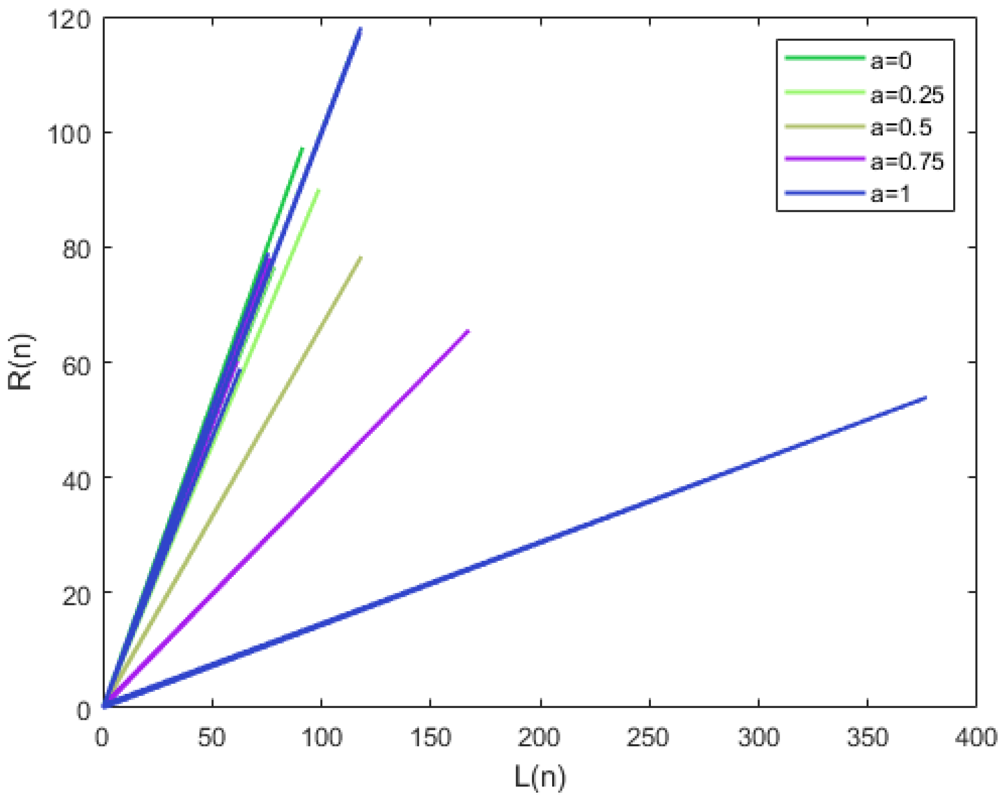
Consider the following third-order fuzzy rational exponential difference equation (1), in which $\eta ,\varphi ,\xi$ are either triangular fuzzy numbers or real constants, depending on the case. We analyze the behavior of the solution $u_n$ under various scenarios using the $\alpha$-cut method. In the following figures, we present the behavior of the fuzzy sequence $u_n$, obtained from the proposed fuzzy difference equation. Since $u_n$ is a fuzzy number, its solution is represented in terms of its $\alpha$-level sets. For a fixed value of $\alpha \in [0,1]$, we denote by $L\left(n\right)$ and $R\left(n\right)$ the left and right endpoints of the $\alpha$-cut of $u_n$, respectively. That is,

$${\left[u_n\right]}_{\alpha }=[L\left(n\right),R\left(n\right)].$$

4.1. Case I: Triangular Fuzzy Parameters and Specific Fuzzy Initial Values

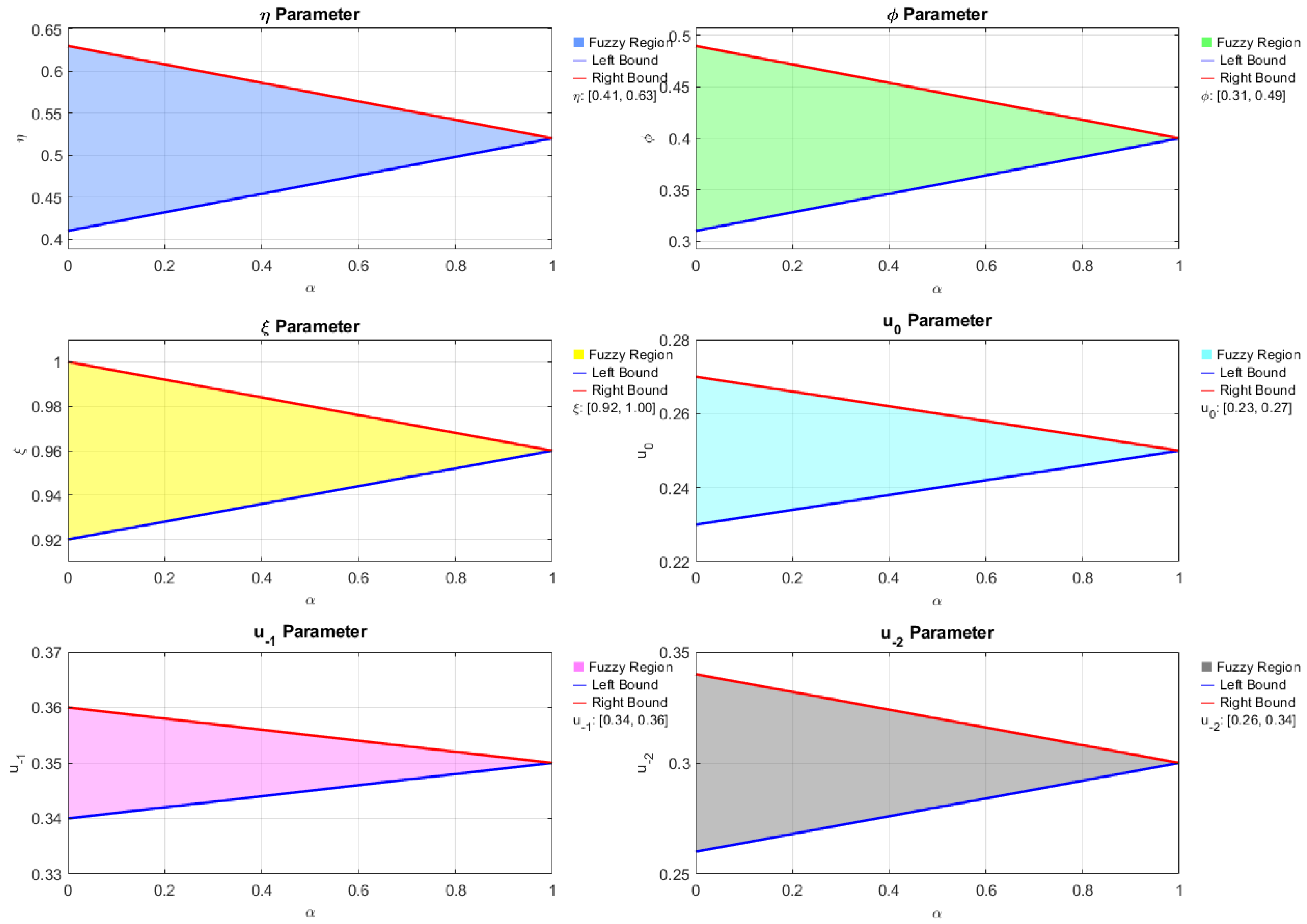
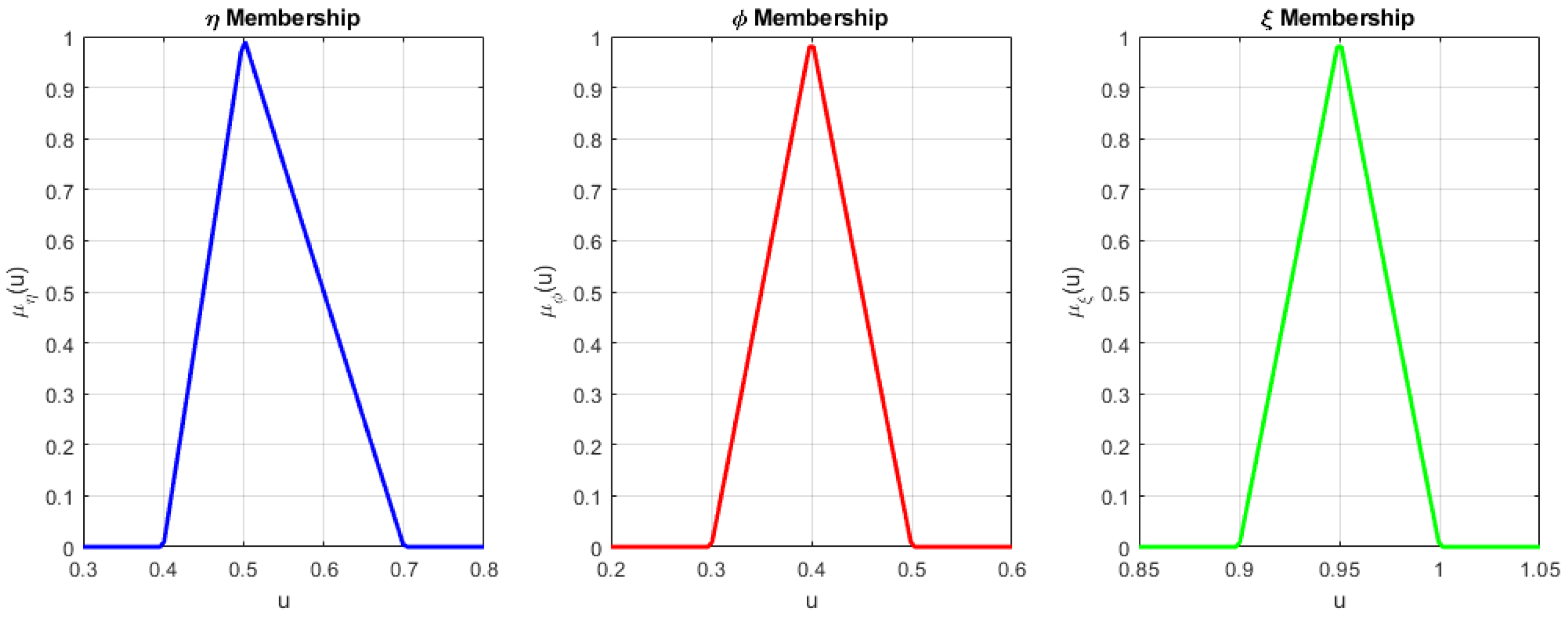
Let $\eta ,\varphi ,\xi$ be triangular fuzzy numbers, and the initial conditions $u_{-2},u_{-1},u_0$ be fuzzy numbers. Membership functions are defined piecewise, and the $\alpha$-cuts are computed in Figure 1, Figure 2, Figure 3 and Figure 4. Using the $\alpha$-cut method, we derive the following pair of parameterized equations:

$$\begin{array}{cc}\hfill L_{n+1,\alpha }& ={\displaystyle \frac{{\eta }_{r,\alpha }{e}^{-L_{n,\alpha }}+{\varphi }_{r,\alpha }{e}^{-L_{n-1,\alpha }}}{{\xi }_{r,\alpha }+R_{n-2,\alpha }}},\hfill \\ \hfill R_{n+1,\alpha }& ={\displaystyle \frac{{\eta }_{l,\alpha }{e}^{-R_{n,\alpha }}+{\varphi }_{l,\alpha }{e}^{-R_{n-1,\alpha }}}{{\xi }_{l,\alpha }+L_{n-2,\alpha }}},\alpha \in (0,1],\hfill \end{array}$$

(64)

where $\eta ,\varphi$, and $\xi$ are the triangular fuzzy number and $u_{-2},u_{-1},u_0$ are the initial conditions; then,

$$\begin{array}{c}\hfill \eta \left(u\right)=\left\{\begin{array}{cc}12.5u-1\hfill & if\mathrm{u}\in [0.4,0.48]\hfill \\ 6.25u-3\hfill & if\mathrm{u}\in [0.48,0.64]\hfill \end{array}\right.,\varphi \left(u\right)=\left\{\begin{array}{cc}10u-3\hfill & if\mathrm{u}\in [0.3,0.4]\hfill \\ -10u+5\hfill & if\mathrm{u}\in [0.4,0.5]\hfill \end{array}\right.\end{array}$$

(65)

$$\begin{array}{c}\hfill \xi \left(u\right)=\left\{\begin{array}{cc}25u-23\hfill & if0.92\le u\le 0.96\hfill \\ -25u+25\hfill & if0.96\le u\le 1\hfill \end{array}\right.,u_0\left(u\right)=\left\{\begin{array}{cc}20u-4\hfill & if0.2\le u\le 0.25\hfill \\ -20u+6\hfill & if0.25\le u\le 0.3\hfill \end{array}\right.\end{array}$$

(66)

$$\begin{array}{c}\hfill u_{-1}\left(u\right)=\left\{\begin{array}{cc}20u-6\hfill & if\mathrm{u}\in [0.3,0.35]\hfill \\ -20u+8\hfill & if\mathrm{u}\in [0.35,0.4]\hfill \end{array}\right.,u_{-2}\left(u\right)=\left\{\begin{array}{cc}20u-5\hfill & if\mathrm{u}\in [0.25,0.3]\hfill \\ -20u+7\hfill & if\mathrm{u}\in [0.3,0.35]\hfill \end{array}\right..\end{array}$$

(67)

Now, from (65)–(67), we get

$$\begin{array}{c}\hfill {\left[\eta \right]}_{\alpha }=[0.4+0.08\alpha ,0.64-0.08\alpha ],{\left[\varphi \right]}_{\alpha }=[0.3+0.1\alpha ,0.5-0.1\alpha ],\end{array}$$

$$\begin{array}{c}\hfill {\left[\xi \left(u\right)\right]}_{\alpha }=[0.92+0.04\alpha ,1-0.04\alpha ],{\left[u_0\right]}_{\alpha }=[0.2+0.25\alpha ,0.3-0.25\alpha ],\end{array}$$

$$\begin{array}{c}\hfill {\left[u_{-1}\right]}_{\alpha }=[0.3+0.5\alpha ,0.4-0.5\alpha ],{\left[u_{-2}\right]}_{\alpha }=[0.25+0.05\alpha ,0.35-0.05\alpha ].\end{array}$$

Consequently, we have

$$\begin{array}{c}\hfill \overline{{\cup }_{\alpha \in (0,1]}{\left[\varphi \right]}_{\alpha }}=[0.3,0.5],\overline{{\cup }_{\alpha \in (0,1]}{\left[\eta \right]}_{\alpha }}=[0.4,0.64]\end{array}$$

$$\begin{array}{c}\hfill \overline{{\cup }_{\alpha \in (0,1]}{\left[\xi \right]}_{\alpha }}=[0.92,1],\overline{{\cup }_{\alpha \in (0,1]}{\left[u_0\right]}_{\alpha }}=[0.2,0.3]\end{array}$$

$$\begin{array}{c}\hfill \overline{{\cup }_{\alpha \in (0,1]}{\left[u_{-1}\right]}_{\alpha }}=[0.3,0.4],\overline{{\cup }_{\alpha \in (0,1]}{\left[u_{-2}\right]}_{\alpha }}=[0.25,0.35].\end{array}$$

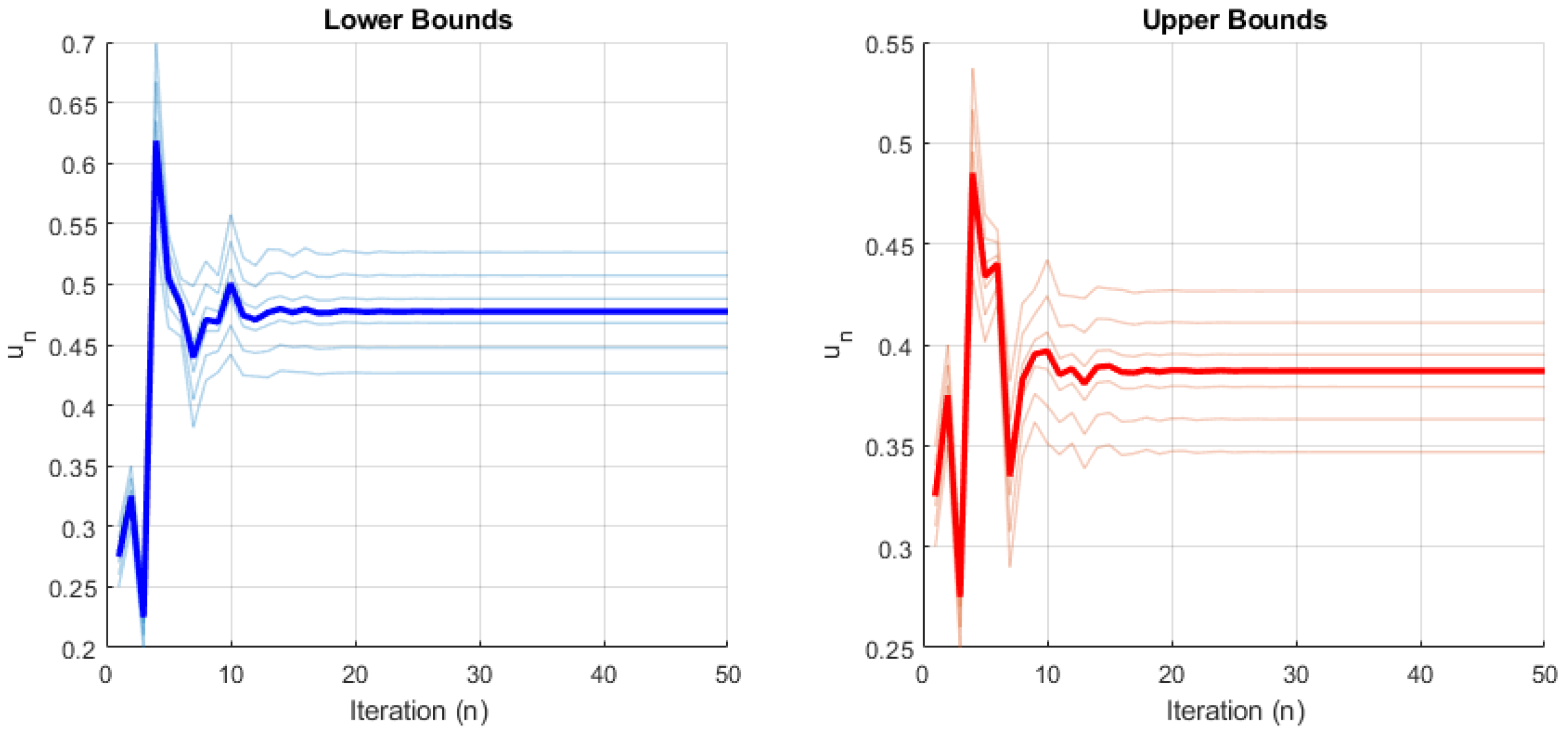
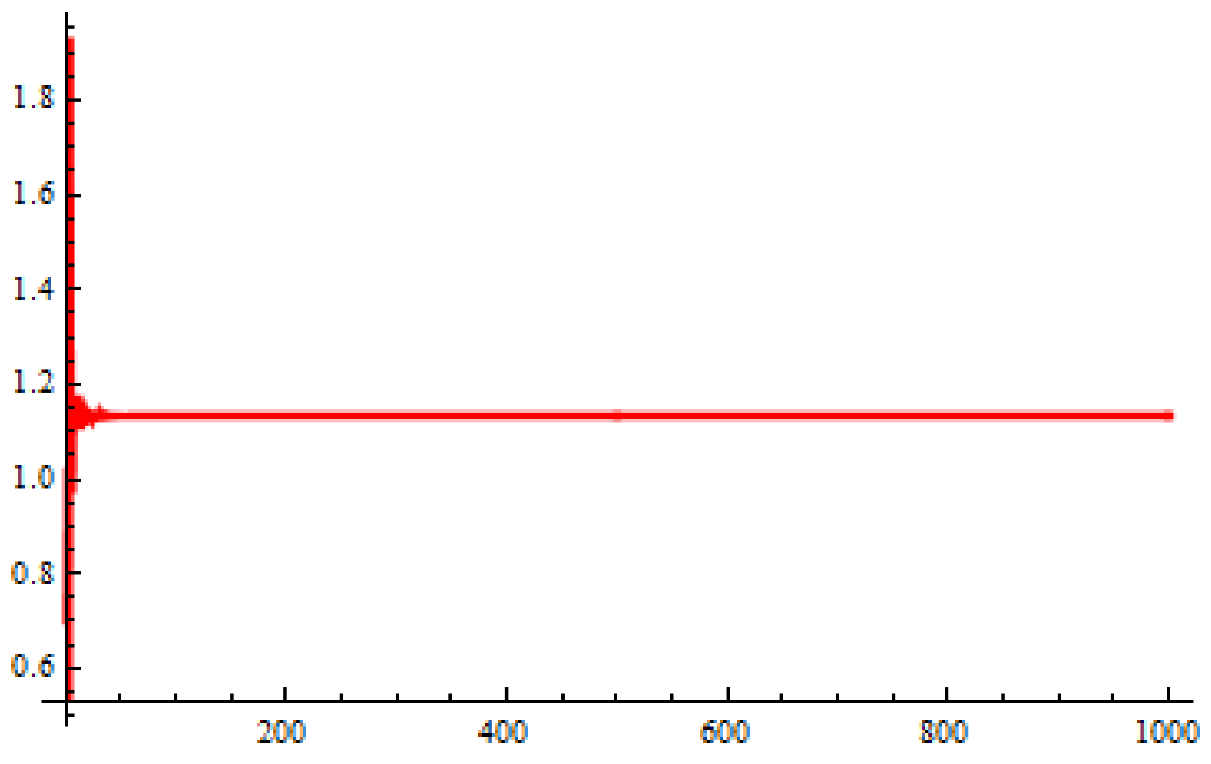
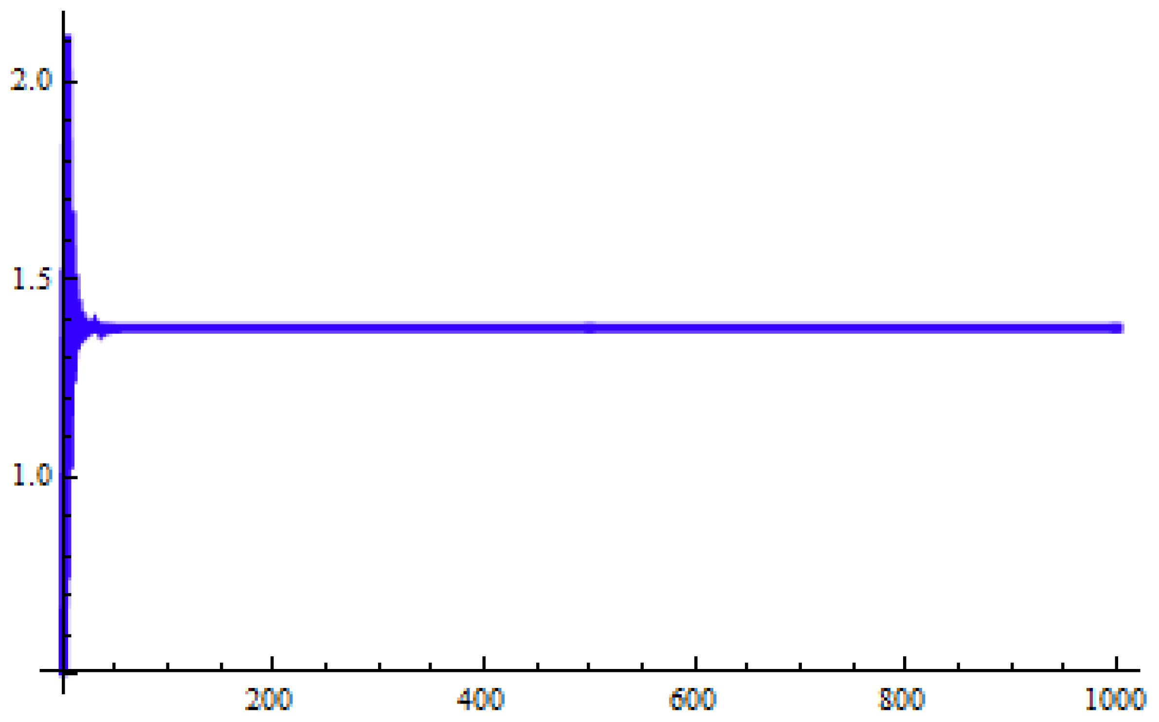
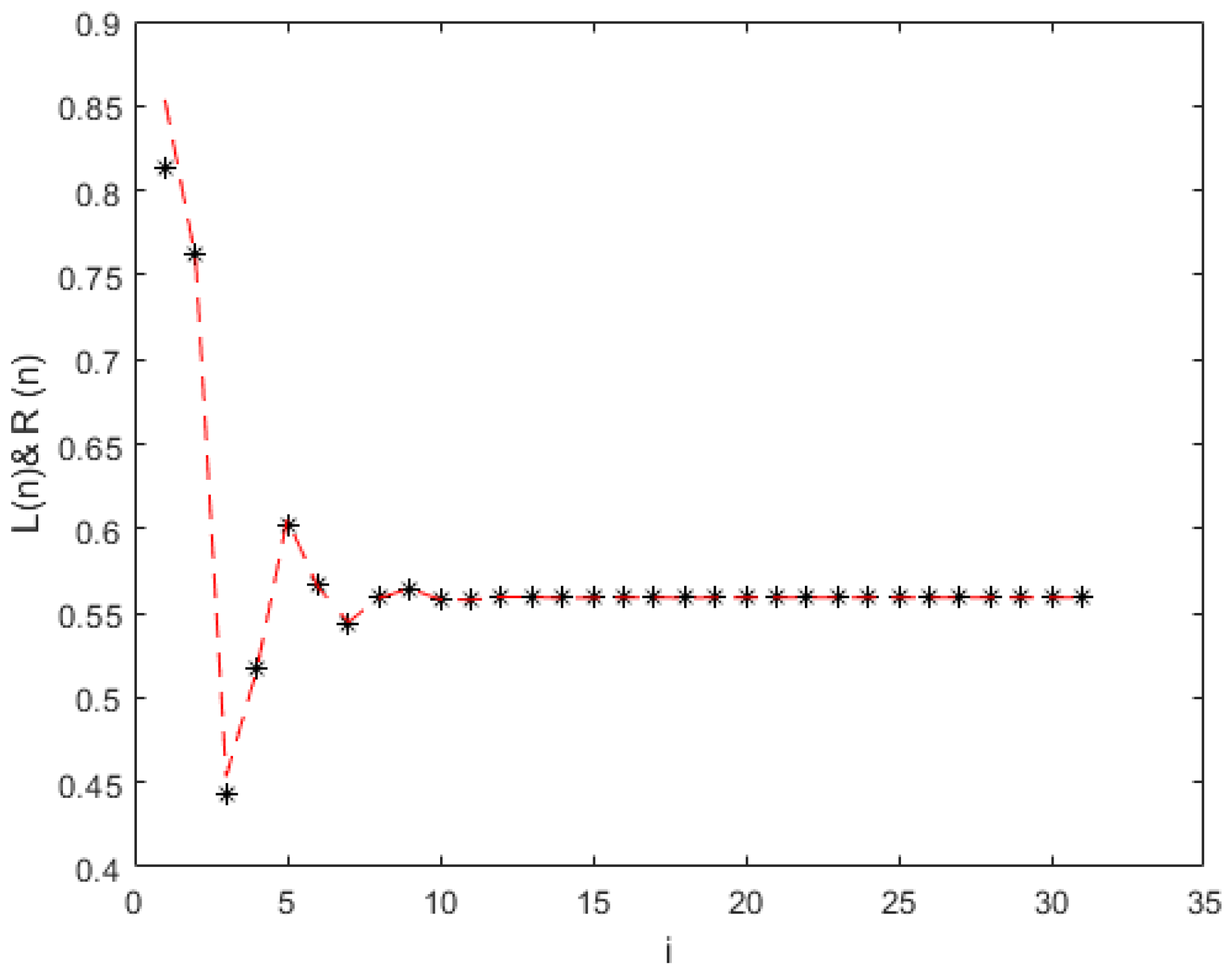
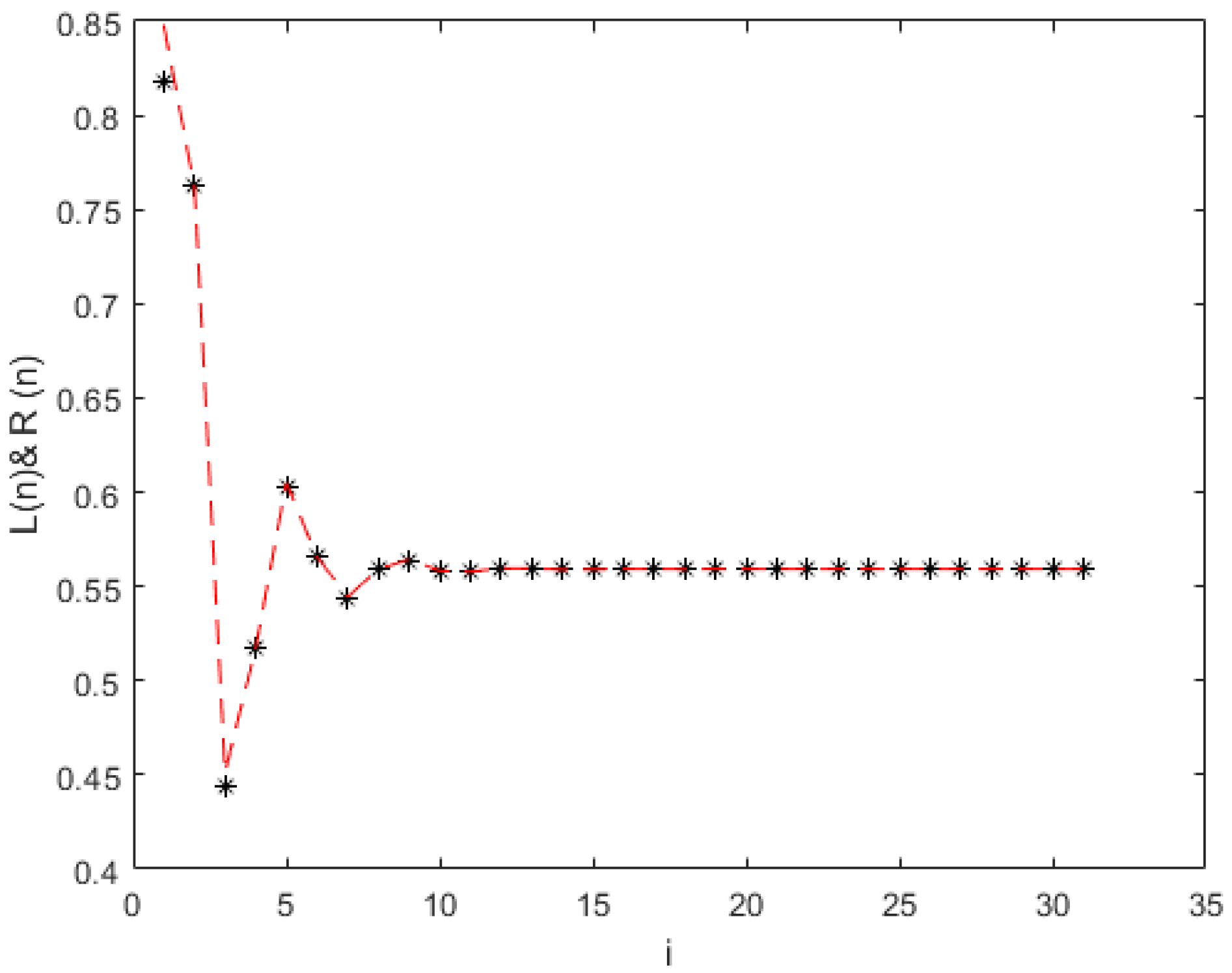
Based on Theorem 5, it can be concluded that every non-negative solution $u_n$ of Equation (1) exists and remains bounded. Moreover, the result possesses a unique equilibrium point, given by $\overline{u}=(0.5591,0.5591,0.5591)$. Additionally, all positive solutions of Equation (1) converge to the equilibrium $\overline{u}$ as $n\to \infty$. This behavior is illustrated in Figure 1, Figure 2, Figure 3, Figure 4 and Figure 5.

In particular, Figure 3 and Figure 4 demonstrate that the positive fuzzy solution $u_n$, characterized by its $\alpha$-cut ${\left[u\right]}_{\alpha }=[L_{n,\alpha },R_{n,\alpha }]$, corresponding to the initial values $u_{-2}=(0.25,0.05,0.35)$, $u_{-1}=(0.3,0.5,0.4)$, and $u_0=(0.2,0.25,0.3)$, converges to the positive equilibrium point $\overline{u}=(0.5591,0.5591,0.5591)$ as $n\to \infty$.

Figure 5 illustrates the dynamic behavior of the fuzzy solution $u_n$ under the given triangular fuzzy number parameters and initial conditions. The convergence to the unique equilibrium point $\overline{u}=(0.5591,0.5591,0.5591)$ is clearly visible. The plot confirms the theoretical results of boundedness and global stability.

4.2. Case II: Modified Fuzzy Parameters and Initial Values

This case employs a new set of triangular fuzzy numbers and different fuzzy initial values. The equation structure remains unchanged, and the same parameterized equations apply. The different fuzzy initial values of $\eta ,\varphi$, and $\xi$ are as follows:

$$\begin{array}{c}\hfill \eta \left(u\right)=\left\{\begin{array}{cc}13u-2.8\hfill & \mathrm{if}u\in [0.4,0.5]\hfill \\ 7u-2.5\hfill & \mathrm{if}u\in [0.5,0.7]\hfill \end{array}\right.,\varphi \left(u\right)=\left\{\begin{array}{cc}11u-2.7\hfill & \mathrm{if}u\in [0.3,0.4]\hfill \\ -9u+4.5\hfill & \mathrm{if}u\in [0.4,0.5]\hfill \end{array}\right.\end{array}$$

(68)

$$\begin{array}{c}\hfill \xi \left(u\right)=\left\{\begin{array}{cc}28u-25.2\hfill & \mathrm{if}0.9\le u\le 0.95\hfill \\ -30u+30\hfill & \mathrm{if}0.95\le u\le 1\hfill \end{array}\right.,\end{array}$$

(69)

with conditions

$$\begin{array}{c}\hfill u_0\left(u\right)=\left\{\begin{array}{cc}22u-4.4\hfill & \mathrm{if}0.2\le u\le 0.25\hfill \\ -18u+5.4\hfill & \mathrm{if}0.25\le u\le 0.3\hfill \end{array}\right.\end{array}$$

(70)

$$\begin{array}{c}\hfill u_{-1}\left(u\right)=\left\{\begin{array}{cc}18u-5.4\hfill & \mathrm{if}u\in [0.3,0.35]\hfill \\ -16u+6.4\hfill & \mathrm{if}u\in [0.35,0.4]\hfill \end{array}\right.\end{array}$$

(71)

$$\begin{array}{c}\hfill u_{-2}\left(u\right)=\left\{\begin{array}{cc}17u-4.25\hfill & \mathrm{if}u\in [0.25,0.3]\hfill \\ -17u+5.95\hfill & \mathrm{if}u\in [0.3,0.35]\hfill \end{array}\right..\end{array}$$

(72)

The $\alpha$-cuts become

$$\begin{array}{cc}\hfill {\left[\eta \right]}_{\alpha }& =[0.4+0.1\alpha ,0.7-0.2\alpha ]\hfill \\ \hfill {\left[\varphi \right]}_{\alpha }& =[0.3+0.1\alpha ,0.5-0.1\alpha ]\hfill \\ \hfill {\left[\xi \right]}_{\alpha }& =[0.9+0.05\alpha ,1-0.05\alpha ]\hfill \\ \hfill [u_0{]}_{\alpha }& =[0.2+0.05\alpha ,0.3-0.05\alpha ]\hfill \\ \hfill [u_{-1}{]}_{\alpha }& =[0.3+0.05\alpha ,0.4-0.05\alpha ]\hfill \\ \hfill [u_{-2}{]}_{\alpha }& =[0.25+0.05\alpha ,0.35-0.05\alpha ]\hfill \end{array}$$

The 3D plot illustrates the dynamic behavior of the fuzzy solution ${\left(u_n\right)}_{\alpha }$ with respect to both the discrete index n and the fuzzy level $\alpha \in [0,1]$. It highlights how the left and right bounds of the $\alpha$-cut evolve. The surface shows convergence trends and potential oscillatory behavior, reflecting the qualitative nature of the fuzzy difference equation. The attractor behavior or boundedness of the trajectories can be visualized for different values of $\alpha$.

Figure 6, Figure 7 and Figure 8 show the behavior of the fuzzy solution $u_n$ for different $\alpha$-levels: $0.2$, $0.4$, and $0.6$. These figures highlight how the fuzzy bounds evolve. As $\alpha$ increases, the fuzziness reduces and the solution approaches closer to the crisp equilibrium.

4.3. Case III: Real Parameters with Fuzzy Initial Bounds

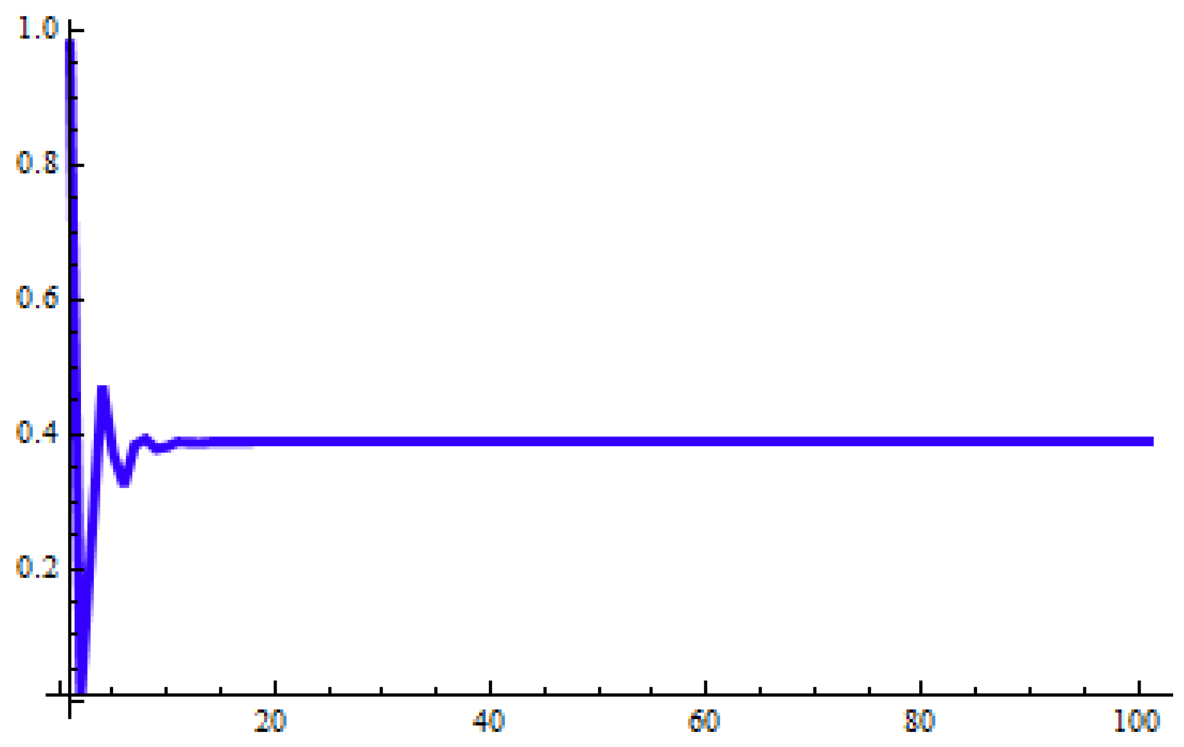
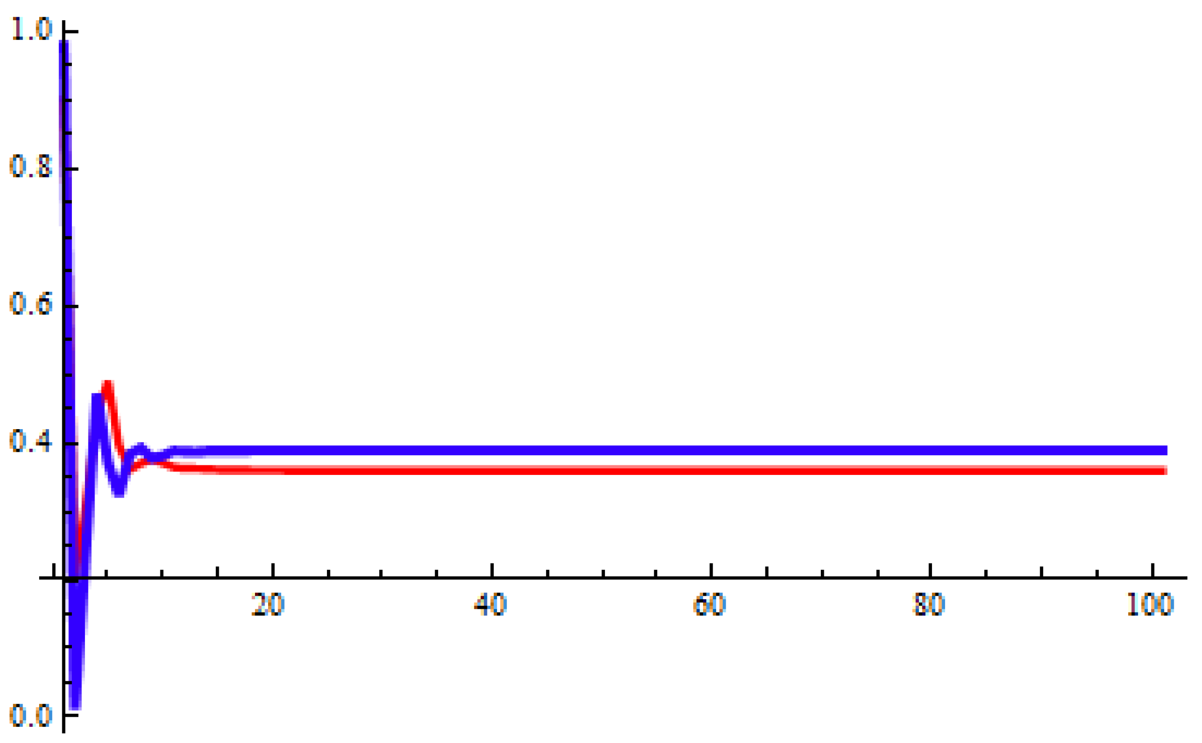
We now consider crisp values for the parameters $\eta =20$, $\varphi =13$, and $\xi =4$, and fuzzy bounds for the following initial conditions:

$$\begin{array}{cc}\hfill L_{-2}& =1.9,L_{-1}=10.9,L_0=0.7,\hfill \\ \hfill R_{-2}& =1.7,R_{-1}=17.8,R_0=0.51.\hfill \end{array}$$

Figure 9, Figure 10 and Figure 11 show that both $L_n$ and $R_n$ converge to a common stable equilibrium, highlighting global asymptotic stability.

4.4. Case IV: Real Parameters with Different Magnitudes

Here, we take $\eta =2.1$, $\varphi =2.4$, and $\xi =2.4$, with

$$\begin{array}{cc}\hfill L_{-2}& =14.9,L_{-1}=17.9,L_0=7.7,\hfill \\ \hfill R_{-2}& =12.9,R_{-1}=15.8,R_0=5.51.\hfill \end{array}$$

Figure 12, Figure 13 and Figure 14 depict the narrowing of the $\alpha$-cut bounds and confirm convergence toward a shared equilibrium value, thus validating the theoretical results.

5. Conclusions

Mathematical modeling serves as a fundamental tool in disciplines such as engineering, ecology, and social sciences for addressing complex real-world problems. While difference equations are effective in representing continuous phenomena, difference equations are more suited to discrete systems. Recently, the use of difference equations in modeling discrete systems has gained significant attention. When uncertainty and vagueness are inherent in these problems, fuzzy set theory becomes a natural extension in the study of difference equations. The field of fuzzy difference equations has already yielded various insightful findings and continues to evolve.

This article focuses on solving a linear fuzzy difference equation characterized by initial conditions which are fuzzy, fuzzy numbers, and fuzzy parameters. Our work further investigates the equilibrium states and their stability in a system modeled by a fuzzy difference equation. The key contributions of this research can be summarized as follows.

Global dynamics and oscillatory behavior of nonlinear fuzzy difference equations with exponential decay are examined using the g-division approach. The existence of positive solutions for Equation (1) is established through qualitative analysis.

(i)

According to Case I, it is shown that Equation (1) admits a bounded and positive fuzzy solution. Additionally, based on Equations (29) and (30), every positive solution $u_n$ can be found to terminate at a unique equilibrium point $\overline{u}$ for any number $n\to \infty$.

(ii)

Similarly, a bounded positive fuzzy solution is guaranteed in Case II. Furthermore, if Conditions (60) and (61) hold, then every positive solution $u_n$ tends to a unique equilibrium point $\overline{u}$ as $n\to \infty$.

The theoretical findings are supported through two numerical simulations. The numerical results validate the theoretical predictions and demonstrate convergence behavior effectively. The results enhance our understanding of fuzzy difference equation-based models in the context of population dynamics and economic systems. For future work, the exploration of fuzzy population dynamics is suggested. Additionally, further qualitative studies—such as investigating invariant intervals and performing bifurcation analysis—may yield deeper insights into the behavior of the given model. Future extensions of this work may explore fractional-order fuzzy difference equations that incorporate memory kernels and long-range dependencies, building upon approaches such as the octonion linear canonical transform [41] and energy-adaptive synchronization of nonlinear neuron models [42]. Integrating fuzzy difference equations with predictive control strategies, such as those driven by kernel-based Lipschitz regression and clustering [43], could enable real-time adaptation in cyber–physical systems.

Moreover, there is potential for applying fuzzy frameworks in the study of low-frequency oscillations in large-scale power networks, particularly those utilizing virtual synchronous generators [44]. Leveraging uncertainty-invariance principles and granular-ball rough set models [45] can enhance decision making in fuzzy environments, especially in systems with dynamic thresholds. Finally, incorporating fast and adaptive clustering techniques based on self-growth maps [46] could significantly improve computational modeling of streaming fuzzy data and real-time feedback-driven systems.

References

1. Wang, C.; Qiu, D.; Shen, Y. Fuzzy Number, Fuzzy Difference, Fuzzy Differential: Theory and Applications. Axioms 2025, 14, 254. [Google Scholar] [CrossRef]
2. Kandel, A.; Byatt, W.J. Fuzzy Differential Equations. In Proceedings of the International Conference on Cybernetics and Society, Tokyo, Japan, 3–7 November 1978. [Google Scholar]
3. Zhang, Q.; Yang, L.; Liao, D. behavior of Solutions to a Fuzzy Nonlinear Difference Equation. Iran. J. Fuzzy Syst. 2012, 9, 1–12. [Google Scholar]
4. Agarwal, R.P. Difference Equations and Inequalities; Marcel Dekker: New York, NY, USA, 1992. [Google Scholar]
5. Kocic, V.L.; Ladas, G. Global Behavior of Nonlinear Difference Equations of Higher Order with Application; Kluwer Academic Publishers: Dordrecht, The Netherlands, 1993. [Google Scholar]
6. Din, Q. Global Behavior of a Plant-Herbivore Model. Adv. Differ. Equ. 2015, 2015, 119. [Google Scholar] [CrossRef]
7. Din, Q.; Khan, K.A.; Nosheen, A. Stability Analysis of a System of Exponential Difference Equations. Discrete Dyn. Nat. Soc. 2014, 2014, 375890. [Google Scholar] [CrossRef]
8. Khan, A.Q.; Qureshi, M.N.; Din, Q. Qualitative Behavior of Two Systems of Second-Order Rational Difference Equations. J. Comput. Anal. Appl. 2015, 18, 1027–1041. [Google Scholar]
9. Khan, A.Q. Global Dynamics of Two Systems of Exponential Difference Equations by Lyapunov Function. Adv. Differ. Equ. 2014, 2014, 97. [Google Scholar] [CrossRef]
10. Kalabusic, S.; Kulenovic, M.R.S.; Pilav, E. Dynamics of a Two-Dimensional System of Rational Difference Equations of Leslie–Gower Type. Adv. Differ. Equ. 2011, 2011, 29. [Google Scholar] [CrossRef]
11. Ozturk, F.; Bozkurt, S.; Ozen, S. On the Difference Equation yn+1 = α + β e y n γ + y n 1 . Appl. Math. Comput. 2006, 181, 1387–1393. [Google Scholar] [CrossRef]
12. Touafek, N.; Elsayed, E.M. On the Solutions of Systems of Rational Difference Equations. Math. Comput. Model. 2012, 55, 1987–1997. [Google Scholar] [CrossRef]
13. Zhang, Q.; Liu, J.; Luo, Z. Dynamical Behavior of a System of Third-Order Rational Difference Equation. Discrete Dyn. Nat. Soc. 2015, 2015, 530453. [Google Scholar] [CrossRef]
14. Zhang, Q.; Yang, L.; Liu, J. Dynamics of a System of Rational Third-Order Difference Equation. Adv. Differ. Equ. 2012, 2012, 136. [Google Scholar] [CrossRef]
15. Deeba, E.Y.; De Korvin, A. Analysis by Fuzzy Difference Equations of a Model of CO2 Level in the Blood. Appl. Math. Lett. 1999, 12, 33–40. [Google Scholar] [CrossRef]
16. Papaschinopoulos, G.; Stefanidou, G. Boundedness and Asymptotic Behavior of the Solutions of a Fuzzy Difference Equation. Fuzzy Sets Syst. 2003, 140, 523–539. [Google Scholar] [CrossRef]
17. Mondal, S.P.; Vishwakarma, D.K.; Saha, A.K. Solution of Second Order Linear Fuzzy Difference Equation by Lagrange’s Multiplier Method. J. Soft Comput. Appl. 2016, 1, 11–27. [Google Scholar]
18. Khastan, A. Fuzzy Logistic Difference Equation. Iran. J. Fuzzy Syst. 2018, 15, 55–66. [Google Scholar]
19. Papaschinopoulos, G.; Papadopoulos, B.K. On the Fuzzy Difference Equation xn+1 = A + B x n . Soft Comput. 2002, 6, 456–461. [Google Scholar] [CrossRef]
20. Papaschinopoulos, G.; Papadopoulos, B.K. On the Fuzzy Difference Equation xn+1 = A + x n x n m . Fuzzy Sets Syst. 2002, 129, 73–81. [Google Scholar] [CrossRef]
21. Khastan, A. New Solutions for First Order Linear Fuzzy Difference Equations. J. Comput. Appl. Math. 2017, 312, 156–166. [Google Scholar] [CrossRef]
22. Zhang, Q.; Lin, F.; Zhong, X. On Discrete Time Beverton–Holt Population Model with Fuzzy Environment. Math. Biosci. Eng. 2019, 16, 1471–1488. [Google Scholar] [CrossRef]
23. Zhang, Q. On Dynamic Behavior of Second-Order Exponential-Type Fuzzy Difference Equation. Fuzzy Sets Syst. 2020, 395, 1–15. [Google Scholar] [CrossRef]
24. Usman, M.; Khaliq, A.; Azeem, M.; Swaray, S.; Kallel, M. The Dynamics and Behavior of Logarithmic Type Fuzzy Difference Equation of Order Two. PLoS ONE 2024, 19, e0309198. [Google Scholar] [CrossRef]
25. Tassaddiq, A.; Tanveer, M.; Usman, M.; Almutairi, D.K.; Alharabi, R. On the Global Dynamics of a Fourth-Order Riccati-Type Exponential Fuzzy Difference Equation. Axioms 2025, 14, 118. [Google Scholar] [CrossRef]
26. Yue, P. Uncertain Numbers. Mathematics 2025, 13, 496. [Google Scholar] [CrossRef]
27. Yang, Y.; Li, H. Neural Ordinary Differential Equations for Robust Parameter Estimation in Dynamic Systems with Physical Priors. Appl. Soft Comput. 2024, 169, 112649. [Google Scholar] [CrossRef]
28. Zhang, Z.; Liu, Z.; Ning, L.; Tian, H.; Wang, B. Belief-Based Fuzzy and Imprecise Clustering for Arbitrary Data Distributions. IEEE Trans. Fuzzy Syst. 2025, 1–13. [Google Scholar] [CrossRef]
29. Shi, J.; Liu, C.; Liu, J. Hypergraph-Based Model for Modeling Multi-Agent Q-Learning Dynamics in Public Goods Games. IEEE Trans. Netw. Sci. Eng. 2024, 11, 6169–6179. [Google Scholar] [CrossRef]
30. Yang, Y.; Zhang, Z.; Zhou, Y.; Wang, C.; Zhu, H. Design of a Simultaneous Information and Power Transfer System Based on a Modulating Feature of Magnetron. IEEE Trans. Microw. Theory Tech. 2023, 71, 907–915. [Google Scholar] [CrossRef]
31. Chen, S.; Wang, Y.; Tian, Z.; Xiao, X.; Xie, X.; Gomis-Bellmunt, O. Understanding a Type of Forced Oscillation in Grid-Forming and Grid-Following Inverter Connected Systems. IEEE Trans. Power Electron. 2025, 40, 11628–11640. [Google Scholar] [CrossRef]
32. Zhang, X.; Yang, X.; He, Q. Multi-Scale Systemic Risk and Spillover Networks of Commodity Markets in the Bullish and Bearish Regimes. N. Am. J. Econ. Financ. 2022, 62, 101766. [Google Scholar] [CrossRef]
33. Luo, K.; Fu, Q.; Liu, X.; Zhao, R.; He, Q.; Hu, B.; Duan, J. Study of Polarization Transmission Characteristics in Nonspherical Media. Opt. Lasers Eng. 2024, 174, 107970. [Google Scholar] [CrossRef]
34. Khastan, A.; Alijani, Z. On the New Solutions to the Fuzzy Difference Equation xn+1 = A + B/xn. Fuzzy Sets Syst. 2019, 358, 64–83. [Google Scholar] [CrossRef]
35. Wang, C.; Su, X.; Liu, P.; Hu, X.; Li, R. On the Dynamics of a Five-Order Fuzzy Difference Equation. J. Nonlinear Sci. Appl. 2017, 10, 3303–3319. [Google Scholar] [CrossRef]
36. Alamin, A.; Mondal, S.P.; Alam, S.; Goswami, A. Solution and Stability Analysis of Non-Homogeneous Difference Equation Followed by Real Life Application in Fuzzy Environment. Sādhanā 2020, 45, 185. [Google Scholar] [CrossRef]
37. Stefanini, L. A Generalization of Hukuhara Difference and Division for Interval and Fuzzy Arithmetic. Fuzzy Sets Syst. 2010, 161, 1564–1584. [Google Scholar] [CrossRef]
38. Lakshmikantham, V.; Vatsala, A.S. Basic Theory of Fuzzy Difference Equations. J. Differ. Equ. Appl. 2002, 8, 957–968. [Google Scholar] [CrossRef]
39. Bede, B. Mathematics of Fuzzy Sets and Fuzzy Logic; Springer: London, UK, 2013. [Google Scholar]
40. Dubois, D.; Prade, H. Possibility Theory: An Approach to Computerized Processing of Uncertainty; Plenum Press: New York, NY, USA, 1998. [Google Scholar]
41. Jiang, N.; Feng, Q.; Yang, X.; He, J.; Li, B. The Octonion Linear Canonical Transform: Properties and Applications. Chaos Solitons Fractals 2025, 192, 116039. [Google Scholar] [CrossRef]
42. Tian, H.; Wang, J.; Ma, J.; Li, X.; Zhang, P.; Li, J. Improved Energy-Adaptive Coupling for Synchronization of Neurons with Nonlinear and Memristive Membranes. Chaos Solitons Fractals 2025, 199, 116863. [Google Scholar] [CrossRef]
43. Xiong, W.; He, D.; Du, H. Learning Economic Model Predictive Control via Clustering and Kernel-Based Lipschitz Regression. J. Frankl. Inst. 2025, 362, 107787. [Google Scholar] [CrossRef]
44. Wang, Y.; Chen, S.; Yang, M.; Liao, P.; Xiao, X.; Xie, X.; Li, Y. Low-Frequency Oscillation in Power Grids with Virtual Synchronous Generators: A Comprehensive Review. Renew. Sustain. Energy Rev. 2025, 207, 114921. [Google Scholar] [CrossRef]
45. Yang, J.; Liu, Z.; Wang, G.; Zhang, Q.; Xia, S.; Wu, D.; Liu, Y. Constructing Three-Way Decision with Fuzzy Granular-Ball Rough Sets Based on Uncertainty Invariance. IEEE Trans. Fuzzy Syst. 2025, 33, 1781–1792. [Google Scholar] [CrossRef]
46. Zhang, Y.; Feng, S.; Wang, P.; Tan, Z.; Luo, X.; Ji, Y.; Cheung, Y. Learning Self-Growth Maps for Fast and Accurate Imbalanced Streaming Data Clustering. IEEE Trans. Neural Netw. Learn. Syst. 2025, 1–13. [Google Scholar] [CrossRef]
Figure 1. Fuzzy solution u n of Equation (1) at α = 0 using the initial conditions u 2 = ( 0.25 , 0.05 , 0.35 ) , u 1 = ( 0.3 , 0.5 , 0.4 ) , and u 0 = ( 0.2 , 0.25 , 0.3 ) . The solution converges to the fuzzy equilibrium point u ¯ = ( 0.5591 , 0.5591 , 0.5591 ) .
Axioms 14 00637 g001
Figure 2. Fuzzy solution u n of Equation (1) at α = 1 confirming the crisp convergence behavior of the system. The endpoints of the α -cut coincide and confirm asymptotic stability.
Axioms 14 00637 g002
Figure 3. Dynamic evolution of fuzzy solution u n from Equation (1) showing both the left and right bounds of α -cuts converging toward the equilibrium point u ¯ as n .
Axioms 14 00637 g003
Figure 4. Behavior of fuzzy solution u n from Equation (1) for multiple iterations and varying α -levels, illustrating convergence and boundedness across all levels of fuzziness.
Axioms 14 00637 g004
Figure 5. Stability region of parameters ( η , ϕ , ξ ) for bounded solutions of (1), showing convergence to equilibrium point u ¯ = ( 0.5591 , 0.5591 , 0.5591 ) .
Axioms 14 00637 g005
Figure 6. Bounded solution and time evolution of (1) with α -cut bounds [ u n ] α .
Axioms 14 00637 g006
Figure 7. Triangular solution and time evolution of (1) with α -cut bounds [ u n ] α .
Axioms 14 00637 g007
Figure 8. A 3D surface plot of α -cut bounds over time and α -levels of Equation (1).
Axioms 14 00637 g008
Figure 9. Stability of the lower α -cut bound L n for η = 20 , ϕ = 13 , ξ = 4 , with initial conditions L 2 = 1.9 , L 1 = 10.9 , L 0 = 0.7 . The plot shows monotonic convergence to a stable equilibrium value.
Axioms 14 00637 g009
Figure 10. Stability of the upper α -cut bound R n under the same parameter settings: η = 20 , ϕ = 13 , ξ = 4 , and initial values R 2 = 1.7 , R 1 = 17.8 , R 0 = 0.51 . The trajectory stabilizes after transient oscillations.
Axioms 14 00637 g010
Figure 11. Combined plot of L n and R n sequences showing the narrowing fuzzy band and convergence toward a common equilibrium point. This supports the theoretical claim of global asymptotic stability of the fuzzy solution.
Axioms 14 00637 g011
Figure 12. Stability of the lower α -cut sequence L n for parameters η = 2.1 , ϕ = 2.4 , ξ = 2.4 with initial values L 2 = 14.9 , L 1 = 17.9 , L 0 = 7.7 . The sequence gradually converges to the equilibrium, indicating global stability.
Axioms 14 00637 g012
Figure 13. Stability of the upper α -cut sequence R n using η = 2.1 , ϕ = 2.4 , ξ = 2.4 and initial values R 2 = 12.9 , R 1 = 15.8 , R 0 = 5.51 . The sequence exhibits convergence behavior consistent with theoretical predictions.
Axioms 14 00637 g013
Figure 14. Combined plot of L n and R n sequences for η = 2.1 , ϕ = 2.4 , ξ = 2.4 , showing the narrowing fuzzy band and convergence toward a shared equilibrium point. This confirms the boundedness and global asymptotic stability of the fuzzy solution.
Axioms 14 00637 g014
Disclaimer/Publisher’s Note: The statements, opinions and data contained in all publications are solely those of the individual author(s) and contributor(s) and not of MDPI and/or the editor(s). MDPI and/or the editor(s) disclaim responsibility for any injury to people or property resulting from any ideas, methods, instructions or products referred to in the content.