Analytical Approximations as Close as Desired to Special Functions

Abstract

We introduce a modern methodology for constructing global analytical approximations of special functions over their entire domains. By integrating the traditional method of matching asymptotic expansions—enhanced with Padé approximants—with differential evolution optimization, a modern machine learning technique, we achieve high-accuracy approximations using elegantly simple expressions. This method transforms non-elementary functions, which lack closed-form expressions and are often defined by integrals or infinite series, into simple analytical forms. This transformation enables deeper qualitative analysis and offers an efficient alternative to existing computational techniques. We demonstrate the effectiveness of our method by deriving an analytical expression for the Fermi gas pressure that has not been previously reported. Additionally, we apply our approach to the one-loop correction in thermal field theory, the synchrotron functions, common Fermi–Dirac integrals, and the error function, showcasing superior range and accuracy over prior studies.

1. Introduction

Many functions encountered in research do not possess desired mathematical properties. Among the many desired properties are integrability, differentiability, invertibility, computational efficiency, simplification by algebraic manipulation with other functions, and the existence of a closed-form expression. We develop a methodology that enables constructing an approximate analytical function that possesses desired qualities, which is as close as desired to the original. These analytical terms alias the objective function for any practical considerations, thus suppressing the unwanted nature of the original function to remain theoretical only.

This paper demonstrates this approach on non-elementary functions relevant to physics. Non-elementary functions are functions that cannot be expressed by a finite number of elementary functions. Instead, they are defined as integrals, infinite sums, or solutions to differential equations. The absence of a closed-form expression can prevent the possibility of qualitative analysis and, in many cases, causes evaluation challenges.

Although accurate evaluation of these functions is possible, it often presents a challenging task that is not directly related to primary research. Not only do their calculations often require knowledge of numerical computation and avoiding numerical instabilities, but they also frequently become the time bottleneck in many computations. In many simulations, integrations, and solutions of differential equations, special functions are evaluated repeatedly an enormous number of times, which accumulates to become the bottleneck of the computations. Additionally, these calculations can lead to memory issues in embedded systems. Numerous efforts have been made to improve the calculation of these functions, e.g., [1], and their computation in embedded systems, e.g, [2]. In parallel, there is a high demand for replacing them with approximations [3,4], as when a simple enough approximation is feasible, it will solve both of these problems at once.

For example, evaluation of the pressure and density of a Fermi gas is carried out by various integrations over the Fermi–Dirac statistics. These integrations must be performed numerically in the general case [5]. These integrations can be an unwanted complication and an extremely inefficient or numerically unstable process. Asymptotic expansions are available only for certain limits. Therefore, an increasing number of terms is needed in the intermediate range to control the error. Constructing a single expression for the entire range not only makes the numerical integration unnecessary, but also enables some qualitative analysis of the entire range at once, which was not possible before. We focus on single-variable functions, and touch upon multivariable functions in Section 4.2.

The remainder of this paper is organized as follows. In Section 2, we provide a comparative review of established approximation techniques, highlighting their respective advantages and limitations. Section 3 presents our novel methodology in detail. To illustrate its practical application, Section 4 offers a comprehensive walk-through example, deriving an approximation for the Fermi gas pressure. We summarize our findings and conclude in Section 5. Finally, the Appendices demonstrate the broad utility of our method, presenting a valuable collection of novel, high-accuracy approximations for several functions critical to physics and applied mathematics. These demonstrations are publicly available in the accompanying Mathematica notebook [6].

2. Known Approximation Techniques

The most widely known method for approximating a function near a given point is the Taylor series expansion [7]. Naively, for approximating a function $f\left(x\right)$ in a given range, one may consider a two-point Taylor expansion [8] which enables interpolation between the points. A more robust structure is the Padé approximant [9], which is defined by a rational function of a given order, i.e., a ratio of two polynomials. It is extensively used in computational mathematics and theoretical physics [10,11,12,13,14,15]. Padé approximants often provide better approximations than Taylor series expansions and may still converge where the Taylor series does not [16]. Thus, when the behavior of a function is known between two points, expansions are often interpolated using two-point Padé approximants [17,18].

Taylor and Padé approximations excel at approximating functions near specific points; however, they often diverge significantly from the target function elsewhere, as they are not designed to uniformly approximate an arbitrary function over the full domain; for instance, they cannot reproduce exponential or logarithmic behavior [19].

Uniform approximation across intervals can be addressed by various minimax approximation methods, which aim to minimize the maximum deviation between the original function and the approximating expression. The most prominent among these is the Remez algorithm, which iteratively finds the optimal uniform approximation. A simpler alternative is Chebyshev interpolation, employing Chebyshev polynomials to approximate a function uniformly within a given interval without the iterative complexity of the Remez algorithm. Nevertheless, these methods remain limited to finite intervals and generally fail to achieve uniform convergence across arbitrarily large domains.

Methods commonly used to achieve uniform convergence over extensive ranges include spline interpolation [20,21,22] and neural network approaches [23,24,25,26]. However, these techniques share significant drawbacks: achieving higher accuracy typically requires increasingly complex models that consume substantially more memory. Specifically, neural network methods suffer from increased computational complexity during evaluation, significantly impacting performance. Additionally, neither interpolation nor neural networks yield simple analytical expressions, thus complicating theoretical analysis.

Therefore, analytical expressions that uniformly approximate the entire domain while maintaining minimal computational complexity are preferable, enabling straightforward theoretical insights.

A well-established technique for constructing global analytic approximations is the method of matching asymptotic expansions [27,28]. This approach expands the target function asymptotically at the boundaries of the desired domain and matches these expansions in an intermediate region to form a global approximation. However, this method lacks uniform accuracy control, with unpredictable deviations between the matched expansions.

Two primary methods address uniform accuracy over the entire domain. The first is a heuristic generalization of Padé approximants [19], capable of achieving better uniformity but lacking precise control over high-level accuracy. The second method, known as the multipoint quasirational approximation technique (MPQA) [29,30,31,32], has demonstrated superior accuracy across various applications. However, it suffers from methodological limitations, primarily in systematically selecting ansatz forms. The coefficients in the MPQA method are determined analytically by matching the higher-order asymptotic expansions between the function and the ansatz. This reflects both a strength and a weakness (compared to this paper’s method): on the one hand, MPQA is analytically tractable; on the other hand, it restricts the choice of ansatz forms to those solvable analytically, and also determines its coefficients by asymptotic matching to power expansions which only approximate the best parameters, and thus limits the overall accuracy.

The goal of this paper is to develop a unified methodology combining the strengths of these approaches to produce simple yet highly accurate approximations. Our systematic procedure will facilitate structured ansatz selection tailored to specific requirements and enable iterative refinement to the desired accuracy level without the restriction of coefficients’ analytical solvability, thus making their refinement easier and more automatic. The coefficients will be determined through numerical minimization of global error to ensure optimal accuracy.

The key approximation techniques are summarized in

Table 1. Comparison of key approximation techniques.

Technique	Pros	Cons	Single Analytical Expression	Global Domain
Taylor and Asymptotic Expansion	Simple to implement; results are often pre-derived and widely available in the literature.	Accurate near the expansion point, but can quickly diverge.	✔	×
Padé Approximants	Superior to Taylor series in terms of convergence across the domain and in its ability to capture pole behaviors.	Cannot reproduce generic functional behaviors (e.g., logarithmic, exponential); can introduce spurious poles.		×
Chebyshev Polynomials and Remez Algorithm	Excellent for limited domains; specialized for achieving uniform accuracy.	Cannot reproduce generic functional behaviors (e.g., logarithmic, exponential).	✔	×
Spline Interpolation	Highly flexible and smooth for interpolating a set of data points.	Results in a piecewise function, not a single analytical expression; can have high memory usage. May oscillate or overfit with noisy data.	×	✔
Neural Networks	Acts as a universal function approximator that can learn from data.	A “black box“ model, not an analytical formula; requires significant data and training; can have long evaluation time and high memory usage.	×	✔
MPQA Approach	Achieves near-optimal approximation parameters. Does not require numerical minimization.	Approximation structure construction/variation is limited by the solvability of asymptotic matching equations.	✔	✔
This Work	Achieves optimal approximation parameters; approximation structure construction/variation is both automatic and unlimited by asymptotic matching solvability.	Requires numerical minimization.

Legend: ✔ = Yes; × = No.

. Related work includes studies on Fermi–Dirac integral combinations [33] and anharmonic oscillator analysis [34].

3. Methodology

The objective is to construct an approximation $\tilde{f}\left(x\right)$ that is as close as desired to a given function, $f\left(x\right)$, in a chosen domain, possibly the entire real axis. We do this by first obtaining the asymptotic expansions of $f\left(x\right)$ at both edges of the range, and then combining them into a single expression that maintains this asymptotic behavior at both edges. The combined expression is naturally only accurate near the edges, while the middle-range accuracy still needs to be tamed. The middle-range accuracy is controlled by adding additional terms that include additional degrees of freedom (DOFs) in the form of coefficients that are determined by numerical minimization of the resultant error.

We denote the range over which $f\left(x\right)$ is approximated as $[x_i,x_f]$. First, we obtain the asymptotic behavior of $f\left(x\right)$ near the edges, i.e., finding the functions $f_i\left(x\right)$ and $f_f\left(x\right)$ that satisfy

$$\underset{x\to x_i}{lim}{\displaystyle \frac{f\left(x\right)}{f_i\left(x\right)}}=1\mathrm{and}\underset{x\to x_f}{lim}{\displaystyle \frac{f\left(x\right)}{f_f\left(x\right)}}=1.$$

(1)

It is important to emphasize that $f_i\left(x\right)$ and $f_f\left(x\right)$ should faithfully reproduce the asymptotic form of $f\left(x\right)$, encompassing all leading terms, including potential divergences. For instance, if $f\left(x\right)$ diverges as $1/(x-x_i)$ or $log|x-x_i|$ near $x_i$, these singular behaviors must be explicitly included in $f_i\left(x\right)$ to maintain the limit condition. The two asymptotics, $f_i$ and $f_f$, are then combined to form the initial structure $f_s\left(x\right)$ that satisfies

$$\underset{x\to x_i}{lim}{\displaystyle \frac{f\left(x\right)}{f_s\left(x\right)}}=\underset{x\to x_f}{lim}{\displaystyle \frac{f\left(x\right)}{f_s\left(x\right)}}=1.$$

(2)

A simple recipe for constructing $f_s$ is by addition:

$$f_s\left(x\right)=g_i\left(x\right)f_i\left(x\right)+g_f\left(x\right)f_f\left(x\right),$$

(3)

where $g_i\left(x\right)$, $g_f\left(x\right)$ are auxiliary functions that control unwanted interference between $f_i\left(x\right)$ and $f_f\left(x\right)$ when it exists. Unwanted interference happens when $f_i\left(x\right)$ is dominant at $x_f$, i.e.,

$$\underset{x\to x_f}{lim}{\displaystyle \frac{f_i\left(x\right)}{f_f\left(x\right)}}\ne 0,$$

(4)

or vice versa, thus preventing satisfaction of the condition in Equation (2). Thus, we require

$$\underset{x\to x_i}{lim}{g}_i\left(x\right)=\underset{x\to x_f}{lim}{g}_f\left(x\right)=1,$$

(5)

which maintains the correct convergence, then determine the remaining behavior based on the interference. When no interference exists, we set $g_i\left(x\right)=g_f\left(x\right)=1$. When interference is present we design the corresponding $g\left(x\right)$ to decay from one to zero towards the other edge. As an example, $f_s\left(x\right)$ of Equation (13) has $g_i\left(x\right)=e^{-x}$ and $g_f\left(x\right)=1$, to fix the unwanted dominance of $f_i\left(x\right)$ over $f_s\left(x\right)$ at $x\to x_f$.

The next step is constructing the final approximation $\tilde{f}\left(x\right)$ on the basis of $f_s\left(x\right)$. This is carried out by performing algebraic manipulations of $f_s\left(x\right)$ that incorporate additional DOFs while maintaining the correct limiting behavior. The objective is to modify the structure to possess the desired properties while striking a balance between simplicity and accuracy. We see that power series, e.g., Equation (14), and Padé approximations, e.g., Equation (15), are excellent candidates as the additional DOFs.

Once the full approximation structure has been set, we proceed into numerical minimization of the parameters to control the accuracy. The relative error of an approximation is defined as follows:

$${\epsilon }_R\left(x\right)=\left|{\displaystyle \frac{f\left(x\right)-\tilde{f}\left(x\right)}{f\left(x\right)}}\right|.$$

(6)

The global accuracy of an approximation, ${\epsilon }_R$, is given by its p-norm ($1\le p$):

$$\parallel {\epsilon }_R{\parallel }_p={\left({\int }_{x_i}^{x_f}{\left|{\displaystyle \frac{\tilde{f}\left(x\right)-f\left(x\right)}{f\left(x\right)}}\right|}^{p}dx\right)}^{{\displaystyle \frac{1}{p}}}.$$

(7)

Minimizing $\parallel {\epsilon }_R{\parallel }_p$ enables the distribution of accuracy efforts uniformly across the entire range. The larger p is, the more the balance shifts towards minimizing the maximal error. We formalize this procedure in Algorithm 1 below:

Algorithm 1 Global Analytical Approximation Construction

Require: Objective function $f\left(x\right)$; desired range $[x_i,x_f]$ (possibly extending to $\pm \infty$).

Ensure: No divergences or singularities exist in the middle of the range; if so, apply the algorithm recursively on subranges excluding them.

1: Obtain the asymptotic expansions of $f\left(x\right)$ at both edges, defining $f_i\left(x\right)$ and $f_f\left(x\right)$ that satisfy Equation (1). Include all leading terms and singular behaviors in $f_i\left(x\right)$ and $f_f\left(x\right)$. 2: Select auxiliary functions $g_i\left(x\right)$ and $g_f\left(x\right)$ to mitigate interference. Choose $g_i\left(x\right)$ and $g_f\left(x\right)$ that decay fast enough to eliminate the interference while converging to one at the other edge. When no interference exists set them both to 1. 3: Construct the initial structure $f_s\left(x\right)=g_i\left(x\right)f_i\left(x\right)+g_f\left(x\right)f_f\left(x\right)$. 4: Construct the final approximation $\tilde{f}\left(x\right)$ from $f_s\left(x\right)$ by algebraic manipulations that maintain the asymptotic behavior unchanged while resulting in the desired form of the approximation. 5: while the achieved $\parallel {\epsilon }_R{\parallel }_{\infty }$ is not sufficient do 6:     Take the last $\tilde{f}\left(x\right)$ and add/change DOF, e.g., adding terms to power series,     or increasing the degree of Padé structure. 7:     Use the described minimization process for the DOF parameters in order to obtain the lowest possible maximal relative error $\parallel {\epsilon }_R{\parallel }_{\infty }$. Evaluate the achieved accuracy. 8: end while

The robustness of the presented method stems from the flexibility to modify the approximation structure, $\tilde{f}\left(x\right)$, as needed until it possesses the required qualities and achieves the desired accuracy. This approach operates under more relaxed restrictions compared to previous methods, as discussed in the Methodology Section. Notably, when $\tilde{f}\left(x\right)$ has zeros within the intermediate range (i.e., not at the endpoints), one can either modify $\tilde{f}\left(x\right)$ to match these zeros exactly or change the minimization objective from relative error to an appropriate measure, for example, the absolute error.

Minimizing a multivariable function is a central challenge in machine learning. As there is no closed way to guarantee the discovery of the global minimum, many algorithms have been developed that search the parameter space for local minima from which the best one is chosen. To make the search as broad as possible, we use both gradient-based and non-gradient-based methods, as either can be suitable for a given case. First, we use the widely known local minimization gradient descent method [35]. To conduct a global search, the gradient descent is initiated from a large number of starting guesses chosen by the Monte Carlo method [36]. For non-gradient-based minimization, we use the differential evolution algorithm [37], which is a specialized global optimization technique that evolves a population of solutions by combining them in specific ways.

For efficient convergence, it is crucial to adopt a sophisticated scoring system, otherwise the minimization may converge impractically slowly or converge to local minima, missing the global one altogether, resulting in a loss of accuracy. The current analysis utilizes a system where p in Equation (7) begins from $p=2$, which represents the standard root mean square, and is gradually taken to ∞. Beginning from a large value of p significantly weakens the convergence, as the larger p is, the weaker the gradient correlates to the global shape of the function, but only to the point of the highest relative error.

By adopting the aforementioned scoring system, all calculations can be performed on a standard personal computer or laptop. In this study, the algorithm was implemented in the Python 3 programming language using the SciPy 1.14.0 [38] library for gradient descent and differential evolution via its built-in functions. Function evaluations utilized the mpmath library [39], which enables the evaluation of functions and their integration with an accuracy and variable range that SciPy does not otherwise support.

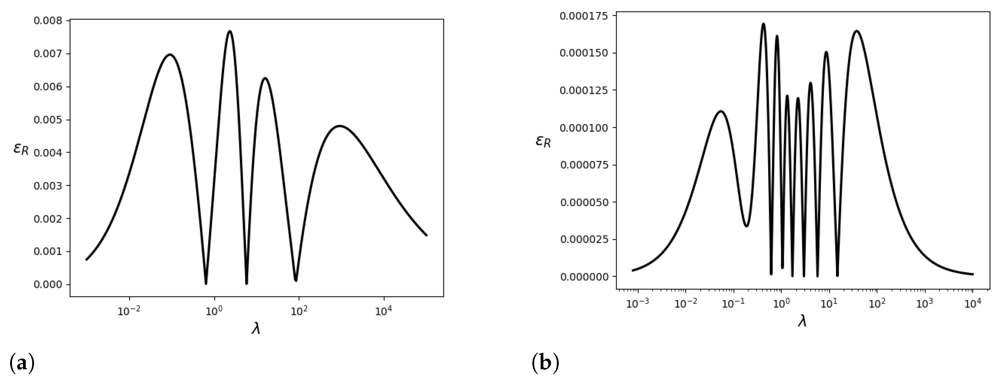
4. Walk-Through Example: Fermi Gas Pressure

As a walk-through example, we choose to construct an approximation for the widely used integral

$$f(\lambda ,\nu )={\int }_1^{\infty }{\displaystyle \frac{{\left(x^2-1\right)}^{\frac{3}{2}}}{e^{\lambda x-\nu }+1}}dx.$$

(8)

It serves as a good example for several reasons. This integral cannot be evaluated analytically [5,40]. It notably represents the pressure of quantum Fermi gas [5], as well as the one-loop thermal correction in quantum field theory [41], which are two important and repeatedly used quantities in physics. Useful expansions in limits of high and low temperature exist; however, they break down in the transition, which has great physical importance.

The pressure of the Fermi gas, in natural units, is given by $p={\displaystyle \frac{g{T}^4}{6{\pi }^2}}{\lambda }^4\times f$, where g is the gas degeneracy factor, T is the temperature, m is the mass, $\mu$ is the chemical potential, and $\lambda \equiv {\displaystyle \frac{m}{T}}$, $\nu \equiv {\displaystyle \frac{\mu }{T}}$.

The one-loop thermal correction in quantum field theory is calculable in terms of the thermal function $J_F$ [41,42,43]:

$$J_F\left(\lambda \right)\equiv {\int }_0^{\infty }{x}^{2}ln\left(1+e^{-\sqrt{x^2+{\lambda }^2}}\right)dx={\displaystyle \frac{{\lambda }^4}{3}}f\left(\lambda ,\mu =0\right).$$

(9)

This thermal function is especially important in phase transitions; therefore, it is relevant for cosmological research on phase transitions in the early universe and beyond the Standard Model physics that might have been at play there [44].

We start from the case of $\mu =0$ by constructing an approximation model for the purpose of providing replacements for negligible-chemical-potential pressure calculation and the thermal function. Then we tackle the case of non-negligible chemical potential, by replacing the integrand with an analytically integrable approximation.

4.1. Zero Chemical Potential

When the chemical potential is either zero or totally negligible, we are left with

$$f\left(\lambda \right)={\int }_1^{\infty }{\displaystyle \frac{{\left(x^2-1\right)}^{\frac{3}{2}}}{e^{\lambda x}+1}}dx.$$

(10)

First, we analyze the asymptotic behavior of f, which is given by [45]:

$$f_i\left(\lambda \right)=f(\lambda \simeq 0)={\displaystyle \frac{7{\pi }^4}{120{\lambda }^4}},$$

(11)

$$f_f\left(\lambda \right)=f(\lambda \simeq \infty )={\displaystyle \frac{3\sqrt{\frac{\pi }{2}}{e}^{-\lambda }}{{\lambda }^{5/2}}}.$$

(12)

Around zero, $f_f$ is negligible compared to $f_i$, i.e., ${lim}_{\lambda \to 0}{\displaystyle \frac{f_f\left(\lambda \right)}{f_i\left(\lambda \right)}}=0$, as needed. For large $\lambda$, $f_i$ is dominant, i.e., ${lim}_{\lambda \to \infty }{\displaystyle \frac{f_i\left(\lambda \right)}{f_f\left(\lambda \right)}}\ne 0$, which creates unwanted overlap. Therefore, to diminish the unwanted overlap, we set $g_i\left(\lambda \right)=e^{-\lambda }$ and $g_f\left(\lambda \right)=1$. Substituting this into Equation (3), we get

$$f_s\left(\lambda \right)=e^{-\lambda }\left({\displaystyle \frac{3\sqrt{\frac{\pi }{2}}}{{\lambda }^{5/2}}}+{\displaystyle \frac{7{\pi }^4}{120{\lambda }^4}}\right).$$

(13)

This initial structure converges at both limits, with a highest relative error of around $0.37$ that occurs in the transition. We proceed by adding DOFs in order to control the error. Adding $\lambda$ powers between ${\displaystyle \frac{5}{2}}$ and 4 keeps the asymptotic behavior intact while also enabling us to reshape the transition range. By fitting both the coefficients and the powers of the two added terms, as can be seen in Figure 1, we improve the maximal relative error to less than one percent, as follows:

$$\tilde{f}\left(\lambda \right)=e^{-\lambda }\left({\displaystyle \frac{111.3}{{\lambda }^{3.05}}}-{\displaystyle \frac{108}{{\lambda }^{3.045}}}+{\displaystyle \frac{3\sqrt{2\pi }}{2{\lambda }^{2.5}}}+{\displaystyle \frac{7{\pi }^4}{120{\lambda }^4}}\right).$$

(14)

Achieving better accuracy is possible through different algebraic manipulation over the basic structure $\tilde{f}$, as long as it maintains the correct convergence at the edges. To incorporate Padé structure into the approximation, we first manipulate $f_s$ into ${\displaystyle \frac{e^{-\lambda }}{{\lambda }^4}}{\displaystyle \frac{\frac{9\pi {\lambda }^8}{2}+\frac{49{\pi }^8}{14400}}{1+{\lambda }^5}}$. Then we add powers to complete it so that it has a full Padé structure. By fitting the coefficients, we enhance the accuracy, as presented in Figure 1, using the final expression:

$$\tilde{f}\left(\lambda \right)={\displaystyle \frac{e^{-\lambda }}{{\lambda }^4}}{\left({\displaystyle \frac{\frac{9\pi {\lambda }^8}{2}+47.95{\lambda }^7+95.3{\lambda }^6+55{\lambda }^5+102.6{\lambda }^4-12{\lambda }^3+37{\lambda }^2+81.1\lambda +\frac{49{\pi }^8}{14400}}{{\lambda }^5-0.33{\lambda }^4+2.18{\lambda }^3-1.597{\lambda }^2+0.522\lambda +1}}\right)}^{0.5}.$$

(15)

This extends and improves upon the previous results for the one-loop thermal correction of [43], which produced a maximum relative error of around 0.05 for the limited range of $0\le {\lambda }^2\le 20$.

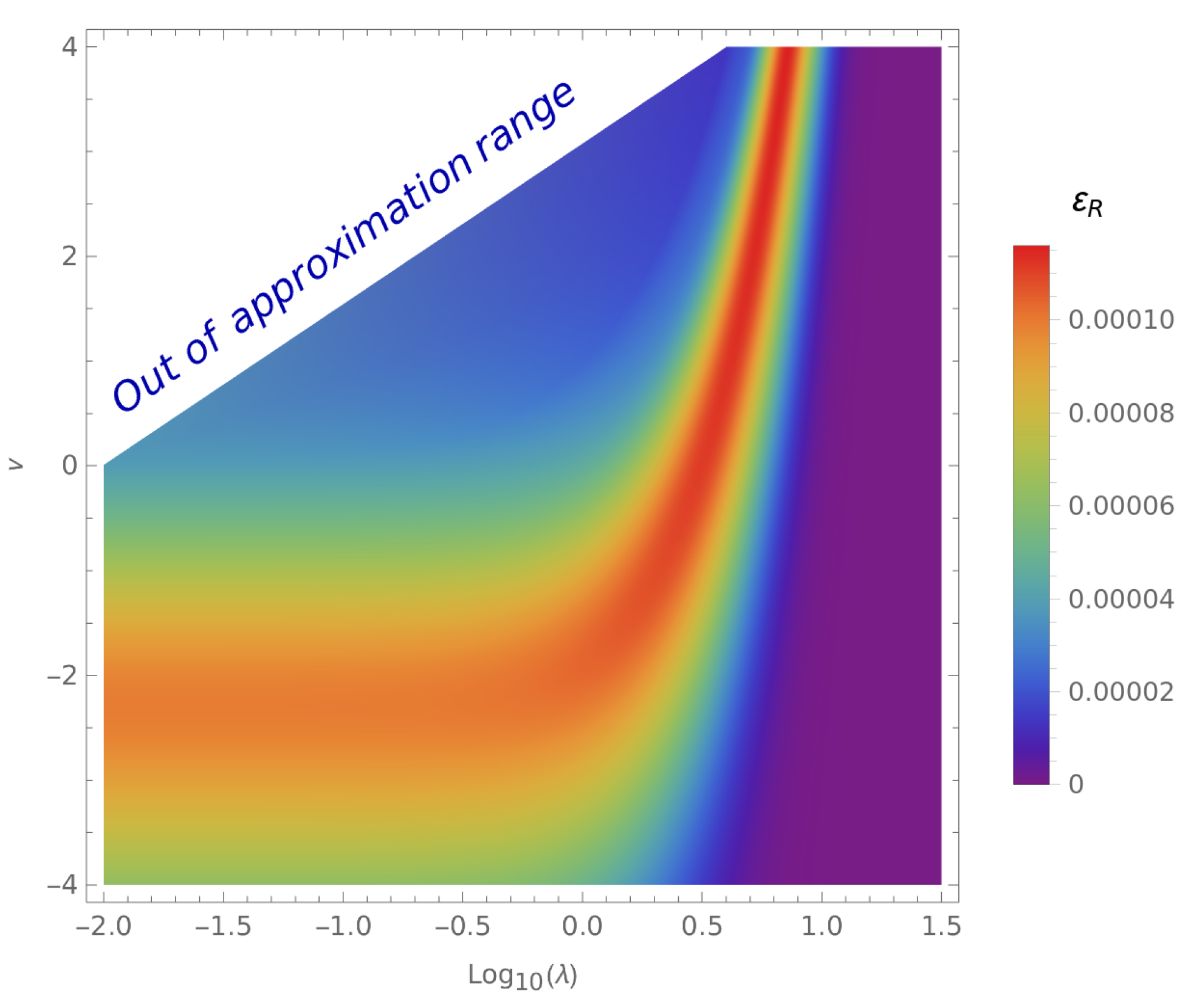
4.2. Nonzero Chemical Potential

Here, we tackle the pressure computation when the chemical potential is not negligible, and thus the pressure becomes a function of two variables—temperature and chemical potential. Our strategy involves keeping the problem one-dimensional by finding a way to approximate f by approximating single-variable functions only.

A common way to evaluate f, which involves one-dimensional expansion only, is Taylor expanding the denominator of Equation (8) around ∞ [40]:

$${\displaystyle \frac{1}{e^x+1}}=\sum _{n=1}^{\infty }{(-1)}^{n+1}{e}^{-nx}.$$

(16)

By using the modified Bessel function of the second kind integral representation,

$$K_{\alpha }\left(z\right)={\displaystyle \frac{\sqrt{\pi }{z}^{\alpha }}{2^{\alpha }\Gamma \left(\alpha +\frac{1}{2}\right)}}{\int }_1^{\infty }{e}^{-zt}{(t^2-1)}^{\alpha -{\displaystyle \frac{1}{2}}}dt,\Re \left(\alpha \right)>-\frac{1}{2},\Re \left(z\right)>0,$$

(17)

it is possible to express the pressure as a sum of Bessel functions. This expansion results in fast convergence only when $\lambda -\nu =x\gg 1$. It requires an unbounded number of terms otherwise. To address this, we replace the common Taylor expansion with an approximation using the presented method. Keeping the approximation analytically integrable, we express the approximation as a sum of exponents only, i.e., ${\sum }_{n=1}^N{c}_n{e}^{-a_{n}x}$. We choose the range of $0\le x<\infty$, which is sufficient as long as $-m\le \mu$. We start by calculating the asymptotic expansions at both edges of the range:

$${\displaystyle \frac{1}{e^x+1}}\underset{x\to 0}{\to }{\displaystyle \frac{1}{2}},{\displaystyle \frac{1}{e^x+1}}\underset{x\to \infty }{\to }{e}^{-x}.$$

(18)

To keep these asymptotic constraints, we take $a_1=c_1=1$, and $1\le a_n$. With this expansion, the integral takes the following form:

$$f(\lambda ,\nu )=\sum _{n=1}^N{\displaystyle \frac{3c_n{e}^{a_n\nu }{K}_2\left(-a_n\lambda \right)}{a_n^2{\lambda }^2}}.$$

(19)

The coefficients $a_n$, $c_n$, and accuracy for various N values of ${\displaystyle \frac{1}{e^x+1}}$ can be seen in Appendix A.2. With that approach, a small number of terms are sufficient for good accuracy across the entire domain.

By replacing ${\displaystyle \frac{1}{e^x+1}}$ with a four-term expansion and simplifying, we get the final expression, which is valid for $-m\le \mu$, presented in Figure 2:

$$\begin{array}{cc}\hfill \tilde{f}(\lambda ,\nu )& ={\displaystyle \frac{1}{{\lambda }^2}}\left(3e^{\nu }{K}_2\left(\lambda \right)-0.8857e^{2.0411\nu }{K}_2\left(2.0411\lambda \right)\right.\hfill \\ \hfill & \left.+1.0814e^{2.787\nu }{K}_2\left(2.787\lambda \right)-0.7283e^{2.92\nu }{K}_2\left(2.92\lambda \right)\right).\hfill \end{array}$$

(20)

In case a closed-form expression is required, one can substitute $K_2\left(x\right)$ by its analytical approximation given in Appendix A.3.

5. Conclusions

A new procedure for constructing global analytical approximations that are accurate over the entire range of the objective function has been demonstrated. These approximations are constructed by first constructing asymptotically convergent structures that serve as a scaffold, into which additional DOFs are blended. These DOFs, which usually come in the form of rational functions, control the accuracy of the approximation by numerical minimization.

First, this procedure has been detailed by directly approximating the pressure of a Fermi gas. This constructed approximation serves as a single expression that is valid across the entire temperature range, thus making the switch between the known low/high-temperature solutions redundant. Then, we expanded it by considering the chemical potential of a nonzero gas as well. This time, through a slightly different approach, we approximated the integrand of the function. By constructing an analytically integrable approximation of the integrand, integration becomes straightforward.

Finally, this procedure has been utilized to produce global approximations for pivotal functions in physics and cosmology that commonly require evaluation at the transition range between the known asymptotics. We chose the key function of the pressure of a quantum Fermi gas as we could not find a known global approximation for this key function and the one-loop correction to the potential in thermal field theory. These functions have been widely discussed in the literature regarding their asymptotic behaviors [40], and dedicated programs for their numerical evaluation have been developed [46]. Moreover, we apply this procedure to functions for which global approximations were previously discussed, as outlined in the Appendices, demonstrating improvements in both precision and range. For enhanced transparency, all plots and approximations presented in this article—along with their full code and precision calculations—are available in the accompanying Mathematica notebook [6].

References

1. Geng, Z.; Abdulah, S.; Sun, Y.; Ltaief, H.; Keyes, D.E.; Genton, M.G. GPU-Accelerated Modified Bessel Function of the Second Kind for Gaussian Processes. In Proceedings of the ISC High Performance 2025 Research Paper Proceedings (40th International Conference), Hamburg, Germany, 10–13 June 2025; pp. 1–12. [Google Scholar]
2. Shah, D.K.; Vyawahare, V.A.; Sadanand, S. Artificial neural network approximation of special functions: Design, analysis and implementation. Int. J. Dyn. Control 2025, 13, 7. [Google Scholar] [CrossRef]
3. Chahrour, I.; Wells, J. Comparing machine learning and interpolation methods for loop-level calculations. SciPost Phys. 2022, 12, 187. [Google Scholar] [CrossRef]
4. Robinson, D.; Avestruz, C.; Gnedin, N.Y. On the minimum number of radiation field parameters to specify gas cooling and heating functions. Open J. Astrophys. 2025, 8, 76. [Google Scholar] [CrossRef]
5. Baumann, D. Cosmology; Cambridge University Press: Cambridge, UK, 2022. [Google Scholar]
6. Orly, A. Supplementary Mathematica Notebook for Analytical Closed-form Expressions, Close as Desired to Special Functions. 2024. Available online: https://github.com/AvivBinyaminOrly/Analytical-Approximations (accessed on 19 May 2024).
7. Arfken, G.B.; Weber, H.J.; Harris, F.E. Mathematical Methods for Physicists: A Comprehensive Guide, 7th ed.; Academic Press: Burlington, MA, USA, 2012. [Google Scholar]
8. López, J.L.; Temme, N.M. Two-Point Taylor Expansions of Analytic Functions. Stud. Appl. Math. 2002, 109, 297–311. [Google Scholar] [CrossRef]
9. Baker, G.A., Jr. Essentials of Padé Approximants; Academic Press: New York, NY, USA, 1975. [Google Scholar]
10. Pozzi, A. Applications of Pade’ Approximation Theory in Fluid Dynamics; World Scientific: Singapore, 1994. [Google Scholar]
11. Prévost, M.; Rivoal, T. Application of Padé approximation to Euler’s constant and Stirling’s formula. Ramanujan J. 2021, 54, 177–195. [Google Scholar] [CrossRef]
12. Bultheel, A. Applications of Padé approximants and continued fractions in systems theory. In Mathematical Theory of Networks and Systems; Springer: Berlin/Heidelberg, Germany, 2005; pp. 130–148. [Google Scholar]
13. Baker, G.A., Jr.; Gammel, J.L. (Eds.) The Padé Approximant in Theoretical Physics; Academic Press: New York, NY, USA, 1971. [Google Scholar]
14. Jordan, K.D.; Kinsey, J.L.; Silbey, R. Use of Pade approximants in the construction of diabatic potential energy curves for ionic molecules. J. Chem. Phys. 1974, 61, 911–917. [Google Scholar] [CrossRef]
15. Basdevant, J.L. The Padé approximation and its physical applications. Fortschritte der Physik 1972, 20, 283–331. [Google Scholar] [CrossRef]
16. Samuel, M.A.; Ellis, J.; Karliner, M. Comparison of the Pade approximation method to perturbative QCD calculations. Phys. Rev. Lett. 1995, 74, 4380. [Google Scholar] [CrossRef] [PubMed]
17. Baker, G.A., Jr.; Graves-Morris, P. Padé Approximants; Cambridge University Press: Cambridge, UK, 1996; Volume 59. [Google Scholar]
18. Bender, C.M.; Orszag, S.A. Advanced Mathematical Methods for Scientists and Engineers I: Asymptotic Methods and Perturbation Theory; Springer: New York, NY, USA, 1999. [Google Scholar]
19. Winitzki, S. Uniform approximations for transcendental functions. In Proceedings of the International Conference on Computational Science and Its Applications (ICCSA 2003), Montreal, QC, Canada, 18–21 May 2003; pp. 780–789. [Google Scholar]
20. Meijering, E. A chronology of interpolation: From ancient astronomy to modern signal and image processing. Proc. IEEE 2002, 90, 319–342. [Google Scholar] [CrossRef]
21. De Boor, C. A Practical Guide to Splines; Springer New York: New York, NY, USA, 1978; Volume 27. [Google Scholar]
22. Phillips, G.M. Interpolation and Approximation by Polynomials; Springer Science & Business Media: Berlin/Heidelberg, Germany, 2003; Volume 14. [Google Scholar]
23. Hornik, K.; Stinchcombe, M.; White, H. Multilayer feedforward networks are universal approximators. Neural Netw. 1989, 2, 359–366. [Google Scholar] [CrossRef]
24. Linka, K.; Schäfer, A.; Meng, X.; Zou, Z.; Karniadakis, G.E.; Kuhl, E. Bayesian physics informed neural networks for real-world nonlinear dynamical systems. Comput. Methods Appl. Mech. Eng. 2022, 402, 115346. [Google Scholar] [CrossRef]
25. Liu, Z.; Yang, Y.; Cai, Q. Neural network as a function approximator and its application in solving differential equations. Appl. Math. Mech. 2019, 40, 237–248. [Google Scholar] [CrossRef]
26. Yang, S.; Ting, T.O.; Man, K.L.; Guan, S.U. Investigation of neural networks for function approximation. Procedia Comput. Sci. 2013, 17, 586–594. [Google Scholar] [CrossRef]
27. Holmes, M.H. Introduction to Perturbation Methods; Springer: New York, NY, USA, 2012; Volume 20. [Google Scholar]
28. O’Malley, R.E., Jr. The Method of Matched Asymptotic Expansions and Its Generalizations. In Historical Developments in Singular Perturbations; Springer: Cham, Switzerland, 2014; pp. 53–121. [Google Scholar]
29. Koch, B.; Olmo, G.J.; Riahinia, A.; Rincón, Á.; Rubiera-Garcia, D. Quasi-normal modes and shadows of scale-dependent regular black holes. arXiv 2025, arXiv:2506.15944. [Google Scholar]
30. Maass, F.; Martin, P.; Olivares, J. Analytic approximation to Bessel function J 0 (x). Comput. Appl. Math. 2020, 39, 222. [Google Scholar] [CrossRef]
31. Maass, F.; Martin, P. Precise analytic approximations for the Bessel function J1 (x). Results Phys. 2018, 8, 1234–1238. [Google Scholar] [CrossRef]
32. Martin, P.; Maass, F. Accurate analytic approximation to the Modified Bessel function of Second Kind K0(x). Results Phys. 2022, 35, 105283. [Google Scholar] [CrossRef]
33. Karasiev, V.V.; Chakraborty, D.; Trickey, S.B. Improved analytical representation of combinations of Fermi–Dirac integrals for finite-temperature density functional calculations. Comput. Phys. Commun. 2015, 192, 114–123. [Google Scholar] [CrossRef]
34. Turbiner, A.V.; del Valle, J.C. Anharmonic oscillator: A solution. J. Phys. A Math. Theor. 2021, 54, 295204. [Google Scholar] [CrossRef]
35. Wang, X.; Yan, L.; Zhang, Q. Research on the Application of Gradient Descent Algorithm in Machine Learning. In Proceedings of the 2021 International Conference on Computer Network, Electronic and Automation (ICCNEA), Xi’an, China, 24–26 September 2021; pp. 11–15. [Google Scholar]
36. Kroese, D.P.; Rubinstein, R.Y. Monte carlo methods. Wiley Interdiscip. Rev. Comput. Stat. 2012, 4, 48–58. [Google Scholar] [CrossRef]
37. Storn, R.; Price, K. Differential evolution–a simple and efficient heuristic for global optimization over continuous spaces. J. Glob. Optim. 1997, 11, 341–359. [Google Scholar] [CrossRef]
38. Virtanen, P.; Gommers, R.; Oliphant, T.E.; Haberland, M.; Reddy, T.; Cournapeau, D.; Burovski, E.; Peterson, P.; Weckesser, W.; Bright, J.; et al. SciPy 1.0: Fundamental Algorithms for Scientific Computing in Python. Nat. Methods 2020, 17, 261–272. [Google Scholar] [CrossRef]
39. Johansson, F. Mpmath: A Python Library for Arbitrary-Precision Floating-Point Arithmetic (Version 0.14). 2010. Available online: http://code.google.com/p/mpmath/ (accessed on 7 January 2024).
40. Khvorostukhin, A.S. Simple way to the high-temperature expansion of relativistic Fermi-Dirac integrals. Phys. Rev. D 2015, 92, 096001. [Google Scholar] [CrossRef]
41. Fowlie, A. A fast C++ implementation of thermal functions. Comput. Phys. Commun. 2018, 228, 264–272. [Google Scholar] [CrossRef]
42. Curtin, D.; Meade, P.; Ramani, H. Thermal resummation and phase transitions. Eur. Phys. J. C 2018, 78, 787. [Google Scholar] [CrossRef]
43. Li, T.; Zhou, Y.F. Strongly first order phase transition in the singlet fermionic dark matter model after LUX. J. High Energy Phys. 2014, 2014, 102. [Google Scholar] [CrossRef]
44. Gouttenoire, Y. Beyond the Standard Model Cocktail: A Modern and Comprehensive Review of the Major Open Puzzles in Theoretical Particle Physics and Cosmology with a Focus on Heavy Dark Matter. arXiv 2023, arXiv:2312.00032. [Google Scholar]
45. Kolb, E.W.; Turner, M.S. The Early Universe; Addison-Wesley: Redwood City, CA, USA, 1990. [Google Scholar]
46. Klajn, B. Exact high temperature expansion of the one-loop thermodynamic potential with complex chemical potential. Phys. Rev. D 2014, 89, 036001. [Google Scholar] [CrossRef]
47. Joyce, W.B.; Dixon, R.W. Analytic approximations for the Fermi energy of an ideal Fermi gas. Appl. Phys. Lett. 1977, 31, 354–356. [Google Scholar] [CrossRef]
48. Selvakumar, C.R. Approximations to Fermi-Dirac integrals and their use in device analysis. Proc. IEEE 1982, 70, 516–518. [Google Scholar] [CrossRef]
49. Koroleva, O.N.; Mazhukin, A.V.; Mazhukin, V.I.; Breslavskiy, P.V. Analytical approximation of the Fermi-Dirac integrals of half-integer and integer orders. Math. Models Comput. Simul. 2017, 9, 383–389. [Google Scholar] [CrossRef]
50. Longair, M.S. High Energy Astrophysics, 3rd ed.; Cambridge University Press: Cambridge, UK, 2011. [Google Scholar]
51. Fouka, M.; Ouichaoui, S. Analytical fits to the synchrotron functions. Res. Astron. Astrophys. 2013, 13, 680. [Google Scholar] [CrossRef]
Figure 1. Relative errors ( ε R ) as a function of λ for Fermi gas pressure approximations. (a) ε R vs. λ for Equation (14). (b) ε R vs. λ for Equation (15).
Axioms 14 00566 g001
Figure 2. Relative errors ( ε R ) for the Fermi gas pressure approximation in Equation (20) at different temperatures and chemical potentials. The white area is outside of the approximation range where 0 m + μ .
Axioms 14 00566 g002