Applied Statistical Modeling Using the Truncated Perk Distribution: Estimation Methods and Multidisciplinary Real-Data Applications

Abstract

In this paper, we propose a new version of the Perk distribution, called the truncated Perk distribution. Fundamental properties of the new distribution are discussed, including moments, the moment generating function, the probability-weighted function, the quantile function, order statistics, Rényi entropy, and Tsallis entropy. In practice, for the estimation of the model parameters, we use seven traditional estimation methods. A simulation study was performed to demonstrate the practical utility of the proposed distribution. In this study, two common estimation methods, MLE and Bayesian estimation, are compared to determine which method provides more accurate and reliable parameter estimates. The potential utility of the truncated Perk model is exhibited through its use on three real datasets. The applications indicate that the truncated Perk distribution can give better fits than some other corresponding distributions.

1. Introduction

Truncated distributions have several applications across various scientific disciplines, particularly in networks of communication, economics, hydrology, materials science, and physics. A truncated distribution is a conditional distribution that arises when the domain size of the original distribution is confined to a narrower location. A truncated distribution arises when incidents occurring either above or below a specified threshold, or outside a defined range, cannot be observed or recorded. Truncated data are a typical and acceptable phenomenon in the field of dependability, particularly when the variable of concern pertains to the failure rates of items. In truncation, information regarding items beyond the limited range is inaccessible. An instance of truncation in manufacturing arises when a sample of things is chosen for analysis from a population that has previously had items excluded for failing to meet established criteria.

Several truncated distributions have been presented by various authors. El Gazar et al. [1,2,3] studied the process of truncation for the inverse power Ailamujia, moment exponential, and inverse power Ishita distributions using their applications in different fields. Elgarhy et al. [4] studied different estimation methods of the inverse power ailamujia and truncated inverse power ailamujia distributions based on progressive type-II censoring scheme. Thiamsorn et al. [5] studied the variant of the truncated Ishita distribution. Singh et al. [6] developed a truncated variant of the Lindley distribution, analyzed its statistical characteristics, and showed that this truncated version provides an enhanced modeling efficacy relative to the Weibull, Lindley, and exponential distributions based on actual data. Also, Almetwally et al. [7] investigated the truncated Cauchy power Weibull-G family, emphasizing the possible relevance and importance of their findings in population research and other fields that involve truncated distributions. Chesneau et al. [8] employed the truncated composite approach to the Burr X distribution, which led to the development of a novel truncated Burr X generated family. The truncated version of the Chris–Jerry model, with its basic properties, is studied by Jabarah et al. [9]. Zaninetti et al. [10] determined that the truncated Pareto distribution outperforms the Pareto distribution in relation to astronomical data. Nadarajah [11] examined several truncated distributions, including the t-distribution and inverted distributions. Furthermore, Nadarajah investigated the beta distribution and the Lévy distribution, which are two separate forms of distributions. Hassan et al. [12] presented the truncated Lomax-G family power Lomax distribution and, in a subsequent study [13], suggested the power truncation of the Lomax-G family. Furthermore, Hussein and Ahmed [14] presented the use of the truncated Gompertz-exponential function on the unit interval, highlighting its distinctive properties and practical applications. Khalaf et al. [15] discussed the truncated Rayleigh Pareto distribution, including its applications. Altawil [16] introduced the truncated Lomax-uniform distribution on the unit interval, clarifying its properties. Elah et al. [17] investigate a novel zero-truncated distribution and its utilization to count datasets. Recently, Nader et al. [18] discussed a new truncated Fréchet-inverted Weibull distribution with many applications in the medical field.

Conversely, recent years have witnessed an increase in studies centered on the innovation of distribution theory, particularly around the Perk (PE) distribution. This dedication arises from the observation of data that diverge from conventional distributions, including gamma, exponential, and Weibull models. In the finance sector, heavy-tailed datasets are frequently poorly represented by conventional models, which results in erroneous risk evaluations and possible financial detriment. Faced with this kind of information, researchers must develop new distributions that more precisely correspond to the noted patterns and which are applicable throughout many fields of expertise. Altering current models has been a prevalent strategy to tackle the diversity present in datasets. In the last twenty years, scholars have investigated novel models by enhancing and modifying current ones.

The PE distribution, originating from the Gompertz–Makeham distribution and developed by [19], is utilized in actuarial science, specifically for the analysis of elderly deaths data, as noted by Richards [20]. Singh et al. [21] also explored the exponentiated Perk distribution. The odd Perk-G distribution family was introduced by Elbatal et al. [22] and is characterized by two scale parameters. Recently, Hussain et al. [23] discussed the inverse power Perk distribution, with its applications in engineering and actuarial fields.

Suppose that a random variable $X$ follows the Perk distribution, then the probability density function (PDF) and cumulative distribution function (CDF) are delineated in the following relations, respectively:

$$f\left(x;\alpha ,\lambda \right)=\alpha \lambda e^{\lambda x}{\displaystyle \frac{\left(1+\alpha \right)}{{\left(1+\alpha e^{\lambda x}\right)}^2}}, \alpha >0 ,\lambda >0, x\ge 0,$$

(1)

$$F\left(x;\alpha ,\lambda \right)=1-\left({\displaystyle \frac{1+\alpha }{1+\alpha e^{\lambda x}}}\right), \alpha >0 ,\lambda >0, x\ge 0.$$

(2)

where $\alpha$ and $\lambda$ are scale parameters.

This paper focuses on a novel truncated distribution, termed the truncated Perk (TPE) distribution, and examines its basic characteristics. It is noteworthy for several reasons:

• From a functional perspective, it is exceedingly straightforward, has merely two parameters, and is still novel in the current literature;
• The associated PDF may exhibit decreasing, right skewness or reversed, J-shaped skewness, while the hazard rate function (HRF) can manifest as increasing or J-shaped skewness. These attributes are advantageous in various contexts, including survival analysis, reliability assessment, and uncertainty analysis;
• This paper analyzes three distinct datasets to provide practical examples that motivate the research. The first dataset is related to economics, whereas the second dataset is related to the environment and the third dataset related to physics. We illustrate that the TPE distribution may serve as a superior alternative to formidable competitors, which confirms the flexibility of the proposed model in dealing with different types of datasets.

Modeling real-world data using flexible statistical distributions is crucial, especially when dealing with truncated, skewed, or bounded datasets. The truncated Perk (TPE) distribution offers such flexibility, which makes it suitable across various fields. In this study, we apply the TPE distribution to three datasets from economics, agriculture, and entomology. These include economic growth indicators with asymmetric patterns, biologically constrained milk yields from SINDI cows, and truncated data on insect counts under different irradiation treatments. In all cases, the TPE distribution provides a superior fit and realistic representation, supporting more accurate inference and decision-making. These applications underscore its adaptability and practical relevance in diverse scientific domains.

The remainder of this paper is structured into the subsequent sections. Section 2 presents the construction of the new truncated model. Numerous fundamental characteristics of the proposed model are delineated in Section 3, supplemented by images and numerical tables as necessary. The estimates of the parameters of the TPE distribution are obtained in Section 4, using seven classical estimation techniques. Section 5 delineates a simulation study to illustrate the adaptability of the new model. Section 6 explained Bayesian estimation for parameters. Section 7 demonstrates the application of the TPE distribution to three categories of real data, highlighting its adaptability. Finally, Section 8 provides conclusive notes, summarizing major findings and prospective avenues for future research.

2. Truncated Perk Model

A novel truncated distribution, referred to as the truncated Perk (TPE) model, is proposed in this section. From the PDF and CDF of the Perk (PE) distribution, shown in Equations (1) and (2), respectively, we can obtain the formula of the PDF and CDF of the TPE distribution, respectively, as follows:

$$f\left(x;\alpha ,\lambda \right)={\displaystyle \frac{K{e}^{\lambda x}}{{\left(1+\alpha e^{\lambda x}\right)}^2}} \mathsf{\alpha },\mathsf{\lambda }>0,0<\mathrm{x}<1,$$

(3)

$$K={\displaystyle \frac{\lambda \left(1+\alpha \right)\left(1+\alpha e^{\lambda }\right)}{\left(e^{\lambda }-1\right)}}$$

and

$$F\left(x;\alpha ,\lambda \right)={\displaystyle \frac{\left(1+\alpha e^{\lambda }\right)\left(e^{\lambda x}-1\right)}{\left(e^{\lambda }-1\right)\left(1+\alpha e^{\lambda x}\right)}}, \alpha ,\lambda >0, 0<x<1.$$

(4)

The probability density function (PDF) of the TPE distribution exhibits notable behavior near the boundaries of the unit interval. Specifically, depending on the parameter values, the density may approach zero, diverge, or remain bounded as $x\to 0$ or $x\to 1$. For instance, under certain configurations, the density tends to zero at both ends, while, in other cases, it may exhibit a sharp increase near one of the boundaries, reflecting the distribution’s flexibility in capturing edge behavior. This behavior can be formally analyzed by setting the limits of the PDF as $x\to 0$ and $x\to 1$, which provide insight into the tail characteristics and boundedness of the model.

It is worth noting that the behavior of the TPE distribution’s probability density function (PDF), when it is set as $x\to 0,$ can be analytically examined. Specifically, under the condition that the parameters satisfy $\alpha >0$, the PDF approaches a finite constant value:

$$\underset{x\to 0}{\lim }f(x)={\displaystyle \frac{K{e}^{\lambda x}}{{\left(1+\alpha \right)}^2}}.$$

This limit indicates that the TPE model is right-bounded and exhibits a well-defined behavior at the lower boundary of the support. Additionally, depending on the specific values of the shape parameters, the TPE distribution’s PDF can exhibit different modalities. For instance, it may be unimodal or monotonically decreasing. This flexibility enhances the usefulness of the model in capturing diverse real-world phenomena

Furthermore, the TPE distribution demonstrates diverse modality patterns depending on the shape parameters. It can be unimodal, exhibiting a single peak, or nearly flat, which allows it to adapt to various empirical data shapes. The location of the mode (if it exists) is sensitive to the interaction between the parameters, and in some instances, numerical methods are required to determine it explicitly. This adaptability makes the TPE distribution particularly suitable for modeling data with skewness or truncated characteristics within the unit interval

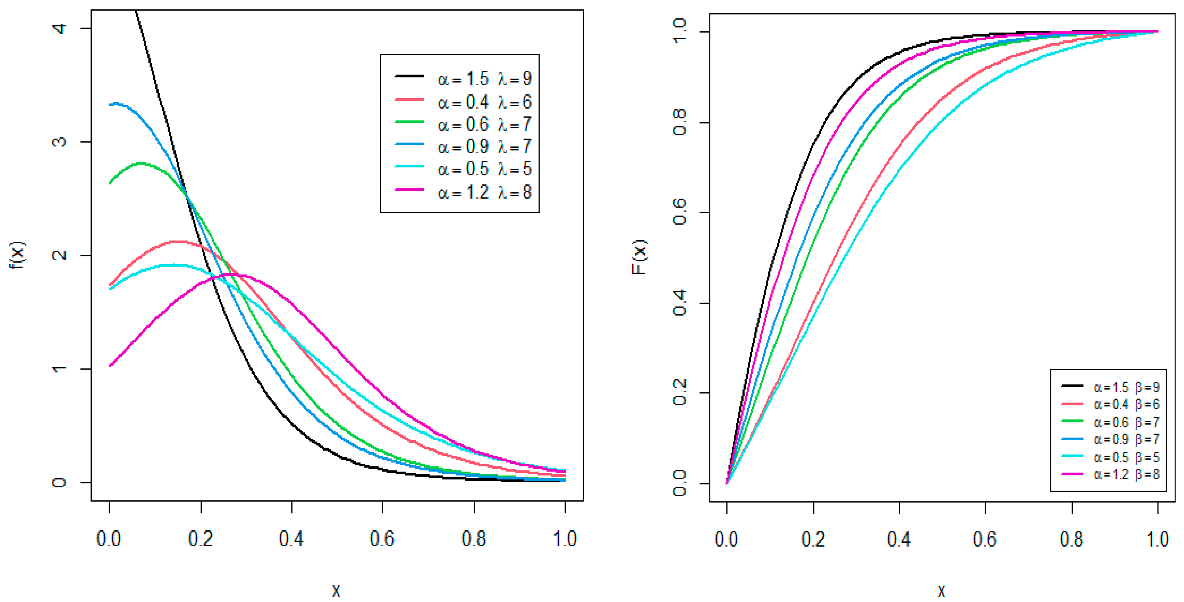
Figure 1 displays a variety of possible shapes of the PDF and CDF of the TPE distribution for some selected values of parameters. It can be detected that the PDF exhibits right skewed and unimodal behavior, while the shape of the CDF increases in size.

According to Equations (3) and (4), the survival function (SF), hazard rate function (HRF), reserved hazard rate function, and cumulative hazard rate function are derived, respectively, as follows:

$$\overline{F}\left(x;\alpha ,\lambda \right)=1-F\left(x;\alpha ,\lambda \right)=1-{\displaystyle \frac{\left(1+\alpha e^{\lambda }\right)\left(e^{\lambda x}-1\right)}{\left(e^{\lambda }-1\right)\left(1+\alpha e^{\lambda x}\right)}},$$

$$h\left(x;\alpha ,\lambda \right)={\displaystyle \frac{ f\left(x;\alpha ,\lambda \right)}{\overline{F}\left(x;\alpha ,\lambda \right)}}={\displaystyle \frac{\frac{K{e}^{\lambda x}}{{\left(1+\alpha e^{\lambda x}\right)}^2} }{1-\frac{\left(1+\alpha e^{\lambda }\right)\left(e^{\lambda x}-1\right)}{\left(e^{\lambda }-1\right)\left(1+\alpha e^{\lambda x}\right)}}},$$

$$\tau \left(x;\alpha ,\lambda \right)={\displaystyle \frac{ f\left(x;\alpha ,\lambda \right)}{F\left(x;\alpha ,\lambda \right)}}={\displaystyle \frac{\lambda \left(1+\alpha \right)e^{\lambda x}}{\left(1+\alpha e^{\lambda x}\right)\left(e^{\lambda x}-1\right)}},$$

$$H\left(x;\alpha ,\lambda \right)=-\ln \left(\overline{F}\left(x;\alpha ,\lambda \right)\right)=-\ln \left(1-{\displaystyle \frac{\left(1+\alpha e^{\lambda }\right)\left(e^{\lambda x}-1\right)}{\left(e^{\lambda }-1\right)\left(1+\alpha e^{\lambda x}\right)}}\right).$$

Figure 2 depicts the survival and hazard rate curves over values of α and λ, showcasing their effectiveness. The HRF plot for the TPE model is evidently growing and has a J-shaped curve.

3. Basic Properties

This section studies the fundamental features of the TPE model such as its moment, moment generating function, coefficients of skewness and kurtosis, probability-weighted function, Renyi entropy, Tsallis entropy, order statistics, and quantile function.

3.1. Moments

Let $X$ be a random variable that follows the TPE distribution with PDF $f_{\mathrm{T}\mathrm{P}\mathrm{E}}\left(x;\alpha ,\lambda \right)$, then the rth moment, say ${\mu }_r^{\prime }$, can be stated as follows:

$${\mu }_r^{\prime }={\int }_0^1{x}^r f_{\mathrm{T}\mathrm{P}\mathrm{E}}\left(x;\alpha ,\lambda \right)dx,$$

(5)

Using Equation (3) in Equation (5), we obtain the following:

$${\mu }_r^{\prime }={\int }_0^1{x}^r {\displaystyle \frac{K{e}^{\lambda x}}{{\left(1+\alpha e^{\lambda x}\right)}^2}}dx.$$

By using the generalized binomial expansions, we obtain the following:

$${\left(1+\alpha e^{\lambda x}\right)}^{-2}=\sum _{i=0}^{\infty }\left(\begin{array}{c}-2\\ i\end{array}\right){\alpha }^i{e}^{i\lambda x}.$$

Therefore, we obtain the following:

$${\mu }_r^{\prime }=\sum _{i=0}^{\infty }\left(\begin{array}{c}-2\\ i\end{array}\right)K{\int }_0^1{x}^r {\alpha }^i{e}^{(i+1)\lambda x}dx.$$

Let $-\mathrm{z}=(i+1)\lambda x$, then ${\mu }_r^{\prime }$ is provided as shown below.

$${\mu }_r^{\prime }=\sum _{i=0}^{\infty }\left(\begin{array}{c}-2\\ i\end{array}\right){\displaystyle \frac{{(-1)}^{r+1}K}{{((i+1)\lambda )}^{r+1}}}{\mathsf{\alpha }}^{\mathrm{i}}\mathsf{\Gamma }\left(r+1,(i+1)\lambda \right),$$

(6)

where $\mathsf{\Gamma }\left(\mathrm{a},\mathsf{\omega }\right)={\int }_0^{\mathrm{a}}{z}^{\omega -1}{e}^{-x}$is the incomplete gamma function.

In particular, the mean and the variance of X are given by:

$${\mu }_1^{\prime }={\sum }_{i=0}^{\infty }\left(\begin{array}{c}-2\\ i\end{array}\right){\displaystyle \frac{K}{{((i+1)\lambda )}^2}}{\mathsf{\alpha }}^{\mathrm{i}}\mathsf{\Gamma }\left(2,(i+1)\lambda \right),$$

$$\begin{array}{cc}\hfill {\sigma }^2={\mu }_2^{\prime }-{\left({\mu }_1^{\prime }\right)}^2& \hfill \\ \hfill =& \left[{\displaystyle \sum _{i=0}^{\infty }}\left(\begin{array}{c}-2\\ i\end{array}\right){\displaystyle \frac{-K}{{\left(\left(i+1\right)\lambda \right)}^3}}{\mathsf{\alpha }}^{\mathrm{i}}\mathsf{\Gamma }\left(3,\left(i+1\right)\lambda \right)\right]\hfill \\ \hfill -& {\left[{\displaystyle \sum _{i=0}^{\infty }}\left(\begin{array}{c}-2\\ i\end{array}\right){\displaystyle \frac{K}{{\left(\left(i+1\right)\lambda \right)}^2}}{\mathsf{\alpha }}^{\mathrm{i}}\mathsf{\Gamma }\left(2,\left(i+1\right)\lambda \right)\right]}^2.\hfill \end{array}$$

Also, the relations of the skewness (${\tau }_1$), the kurtosis (${\tau }_2$), and the coefficient of variation (${\tau }_3$) for the TPE distribution can be written as follows:

$${\tau }_1={\displaystyle \frac{{\mu }_3^{\prime }-3{\mu }_1^{\prime }{\mu }_2^{\prime }+{({\mu }_1^{\prime })}^3}{{({\sigma }^2)}^{\frac{3}{2}}}},{\tau }_3={\displaystyle \frac{{({\sigma }^2)}^{\frac{1}{2}}}{{\mu }_1^{\prime }}},$$

$${\tau }_2={\displaystyle \frac{{\mu }_1^{\prime }-4{\mu }_1^{\prime }{\mu }_3^{\prime }+6{\mu }_2^{\prime }{({\mu }_1^{\prime })}^2-3{({\mu }_1^{\prime })}^4}{{({\sigma }^2)}^2}}.$$

Table 1. Numerical values for the TPE moments with coefficients of ${\tau }_1$, ${\tau }_2$, and ${\tau }_3.$

Parameters		Measures
$\mathit{\alpha }$	$\mathit{\lambda }$	${\mathit{\mu }}_1$	${\mathit{\mu }}_2$	${\mathit{\mu }}_3$	${\mathit{\mu }}_4$	${\mathit{\sigma }}^2$	${\mathit{\tau }}_1$	${\mathit{\tau }}_2$	${\mathit{\tau }}_3$
1.5	0.2	0.4959	0.3292	0.2462	0.1966	0.0833	0.0171	1.8010	0.5819
	0.5	0.4869	0.3199	0.2379	0.1891	0.0829	0.0544	1.8079	0.5914
	0.8	0.4749	0.3078	0.2267	0.1791	0.0822	0.1041	1.8244	0.6037
	1	0.4656	0.2983	0.2181	0.1714	0.0815	0.1431	1.8425	0.6132
2.5	0.2	0.4922	0.3255	0.2430	0.1937	0.0833	0.0324	1.8019	0.5862
	0.5	0.4783	0.3115	0.2304	0.1825	0.0828	0.0904	1.8144	0.6016
	0.8	0.4621	0.2955	0.2159	0.1697	0.0819	0.1577	1.8418	0.6192
	1	0.4504	0.2839	0.2056	0.1606	0.0809	0.2067	1.8702	0.6319
3.5	0.2	0.4902	0.3235	0.2412	0.1922	0.0832	0.0408	1.8027	0.5886
	0.5	0.4736	0.3071	0.2264	0.1791	0.0827	0.1096	1.8192	0.6072
	0.8	0.4554	0.2891	0.2104	0.1649	0.0817	0.1858	1.8538	0.6275
	1	0.4426	0.2766	0.1993	0.1552	0.0807	0.2397	1.8885	0.6417
5	0.2	0.4885	0.3218	0.2396	0.1908	0.0832	0.0480	1.8035	0.5906
	0.5	0.4697	0.3033	0.2231	0.1761	0.0826	0.1259	1.8239	0.6119
	0.8	0.4498	0.2838	0.2058	0.1610	0.0815	0.2095	1.8654	0.6345
	1	0.4361	0.2705	0.1941	0.1508	0.0804	0.2674	1.9060	0.6501
7	0.2	0.4872	0.3205	0.2385	0.1898	0.0832	0.0534	1.8042	0.5921
	0.5	0.4669	0.3005	0.2206	0.1740	0.0825	0.1380	1.8279	0.6154
	0.8	0.4457	0.2799	0.2025	0.1581	0.0813	0.2268	1.8748	0.6397
	1	0.4314	0.2662	0.1904	0.1476	0.0801	0.2876	1.9199	0.6562

provides a numerical depiction of the initial four moments, variance (${\sigma }^2$), coefficients of skewness (${\tau }_1$), kurtosis (${\tau }_2$), and variation (${\tau }_3$) for different parameter values. The results reveal that, for a fixed value of $\lambda$, increasing α leads to a consistent increase in all moment-related measures, including the mean and variance. In contrast, the skewness (${\tau }_1$) and kurtosis (${\tau }_2$) coefficients exhibit a decreasing trend as $\mathsf{\alpha }$ increases, indicating a tendency toward a more symmetric and less peaked distribution. These patterns suggest that the parameter α plays a significant role in shaping the distribution’s tail behavior and overall shape. Also, 3D plots of the measurements for ${\mu }_1$, ${\sigma }^2$, ${\tau }_1$, and ${\tau }_2$ are presented in Figure 3 for further clarification and elucidation. Figure 3 presents three-dimensional charts depicting the variance and mean of the TPE distribution.

3.2. Moment-Generating Function

The MGF of the TPE distribution is derived using the PDF of Equation (3) in Equation (7), as follows:

$${\mathrm{M}}_{\mathrm{X}}\left(\mathrm{t}\right)=\mathrm{E}\left({\mathrm{e}}^{\mathrm{t}\mathrm{x}}\right)={\int }_0^1{\mathrm{e}}^{\mathrm{t}\mathrm{x}} f_{\mathrm{T}\mathrm{P}\mathrm{E}}\left(x;\alpha ,\lambda \right)dx .$$

(7)

Then, by using Exponential Expansion, we obtain the following:

$${\mathrm{M}}_{\mathrm{X}}\left(\mathrm{t}\right)=\sum _{\mathrm{r}=0}^{\mathrm{\infty }}{\displaystyle \frac{{\mathrm{t}}^{\mathrm{r}}}{\mathrm{r}!}}{\int }_0^1{x}^r f_{\mathrm{T}\mathrm{P}\mathrm{E}}\left(x;\alpha ,\lambda \right)dx=\sum _{\mathrm{r}=0}^{\mathrm{\infty }}{\displaystyle \frac{{\mathrm{t}}^{\mathrm{r}}}{\mathrm{r}!}} {\mu }_r^{\prime }.$$

By using Equation (6), the MGF of the TPE distribution is given as follows:

$${\mathrm{M}}_{\mathrm{X}}\left(\mathrm{t}\right)=\sum _{\mathrm{r}=0}^{\mathrm{\infty }}\sum _{i=0}^{\infty }\left(\begin{array}{c}-2\\ i\end{array}\right){\displaystyle \frac{{\left(-1\right)}^{r+1}K {\mathrm{t}}^{\mathrm{r}}}{\mathrm{r}!{\left(\left(i+1\right)\lambda \right)}^{r+1}}}{\mathsf{\alpha }}^{\mathrm{i}}\mathsf{\Gamma }\left(r+1,\left(i+1\right)\lambda \right).$$

3.3. Probability-Weighted Moment

The probability-weighted moment (PWM) approach is commonly used for estimating parameters in distributions that lack a straightforward inverse form. First introduced in [24], this method has gained significant recognition in hydrological studies for estimation purposes. The PWM of the TPE distribution is obtained as follows:

$${\phi }_{\mathrm{P}\mathrm{W}\mathrm{M}}\left(x\right)=E\left(x^r{F}^m\left(x;\alpha ,\lambda \right)\right)={\int }_0^1{x}^r F^m\left(x;\alpha ,\lambda \right)f\left(x;\alpha ,\lambda \right)dx.$$

(8)

By substituting Equations (3) and (4) into Equation (8), we obtain the following:

$${\phi }_{\mathrm{P}\mathrm{W}\mathrm{M}}\left(x\right)={\int }_0^1\Omega (\alpha ,\lambda )x^r e^{\lambda x}{\displaystyle \frac{{\left(e^{\lambda x}-1\right)}^m}{{\left(1+\alpha e^{\lambda x}\right)}^{m+2}}}dx,$$

(9)

where ${\Omega (\alpha ,\lambda )=K\left[{\displaystyle \frac{\left(1+\alpha e^{\lambda }\right)}{\left(e^{\lambda }-1\right)}}\right]}^m$.

For any real number $a,b>0$ and $\left|\epsilon \right|<1$, the generalized binomial series is defined as follows:

${(a+b)}^{\epsilon }={\sum }_{i=0}^{\mathrm{\infty }}\left(\begin{array}{c}\epsilon \\ i\end{array}\right)a^{\epsilon -i}{b}^i$. Then, by using this series, we obtain the following:

$${\left(e^{\lambda x}-1\right)}^m=\sum _{i=0}^{\infty }\left(\begin{array}{c}m\\ i\end{array}\right){(-1)}^{m-i}{e}^{i\lambda x}$$

and

$${\left(1+\alpha e^{\lambda x}\right)}^{-m-2}=\sum _{j=0}^{\infty }\left(\begin{array}{c}-m-2\\ j\end{array}\right){\alpha }^j{e}^{j\lambda x} .$$

By substituting in Equation (9), we obtain the following:

$${\phi }_{\mathrm{P}\mathrm{W}\mathrm{M}}(y)=\sum _{i=j=0}^{\infty }\left(\begin{array}{c}m\\ i\end{array}\right)\left(\begin{array}{c}-m-2\\ j\end{array}\right){(-1)}^{m-i}\Omega (\alpha ,\lambda ){\int }_0^1{x}^r e^{(i+j+1)\lambda x}dx.$$

By using the incomplete Gamma function, the PWM is obtained as follows:

$${\phi }_{\mathrm{P}\mathrm{W}\mathrm{M}}(y)={\sum }_{i=j=0}^{\infty }\left(\begin{array}{c}m\\ i\end{array}\right)\left(\begin{array}{c}-m-2\\ j\end{array}\right){\displaystyle \frac{{(-1)}^{r+m-i+1}}{{((i+j+1)\lambda )}^{r+1}}}\Omega (\alpha ,\lambda ){\alpha }^j\mathsf{\Gamma }\left((i+j+1)\lambda ,r+1\right).$$

3.4. Renyi Entropy

Renyi entropy, proposed by Renyi [25], measures the variation in uncertainty in a distribution. The Renyi entropy is defined as follows:

$$\mathrm{R}\mathrm{E}\left(\mathsf{\eta }\right)={\displaystyle \frac{1}{1-\mathsf{\eta }}}\log \left[{\int }_0^1{f}^{\eta }\left(x\right)dx\right]={\displaystyle \frac{1}{1-\mathsf{\eta }}}\log \left[{\int }_0^1{\displaystyle \frac{K^{\mathsf{\eta }}{e}^{\mathsf{\eta }\lambda x}}{{\left(1+\alpha e^{\lambda x}\right)}^{2\mathsf{\eta }}}}\mathrm{d}\mathrm{x}\right].$$

For any real number a,b > 0 and |ε| < 1, the generalized binomial series is defined as follows:

$${(a+b)}^{\epsilon }=\sum _{i=0}^{\infty }\left(\begin{array}{c}\epsilon \\ i\end{array}\right)a^{\epsilon -i}{b}^i.$$

Then, we obtain the following:

$$\mathrm{R}\mathrm{E}(\mathsf{\eta })={\displaystyle \frac{1}{1-\mathsf{\eta }}}\log \left[\sum _{\mathrm{i}=0}^{\mathrm{\infty }}\left(\begin{array}{c}-2\mathsf{\eta }\\ \mathrm{i}\end{array}\right)K^{\mathsf{\eta }}{\int }_0^1{\alpha }^i{e}^{(i+\eta )\lambda x}\mathrm{d}\mathrm{x}\right].$$

Therefore, the Renyi entropy is developed as follows:

$$\mathrm{R}\mathrm{E}(\mathsf{\eta })={\displaystyle \frac{1}{1-\mathsf{\eta }}}\log \left[\sum _{\mathrm{i}=0}^{\mathrm{\infty }}\left(\begin{array}{c}-2\mathsf{\eta }\\ \mathrm{i}\end{array}\right){\displaystyle \frac{K^{\mathsf{\eta }}{\alpha }^i}{(i+\mathsf{\eta })\lambda }}(e^{(i+\eta )\lambda }-1)\right].$$

3.5. Tsallis Entropy

Tsallis [26] introduced an entropy called Tsallis entropy for generalizing standard statistical mechanics which is defined as follows:

$$\mathrm{T}\mathrm{E}\left(\mathsf{\rho }\right)={\displaystyle \frac{1}{1-\mathsf{\rho }}}\log \left[1-{\int }_0^1{f}^{\rho }\left(x\right)dx\right].$$

For any real number a,b > 0 and |ε| < 1, the generalized binomial series is defined as follows:

$${(a+b)}^{\epsilon }=\sum _{i=0}^{\infty }\left(\begin{array}{c}\epsilon \\ i\end{array}\right)a^{\epsilon -i}{b}^i.$$

Therefore, Tsallis entropy is given as follows:

$$\mathrm{T}\mathrm{E}(\mathsf{\rho })={\displaystyle \frac{1}{1-\mathsf{\rho }}}\log \left[1-\sum _{\mathrm{i}=0}^{\mathrm{\infty }}\left(\begin{array}{c}-2\mathsf{\rho }\\ \mathrm{i}\end{array}\right){\displaystyle \frac{K^{\mathsf{\rho }}{\alpha }^i}{(i+\mathsf{\rho })\lambda }}(e^{(i+\mathsf{\rho })\lambda }-1)\right].$$

3.6. Order Statistics

Assume that $X_1, X_2, \dots \dots ,X_n$is a random sample of size $n$ drawn from the TPE distribution with PDF and CDF as defined in Equation (3) and Equation (4), respectively. Next, order statistics are indicated by $X_{(1)}, X_{(2)}, \dots \dots ,X_{(n)},$where $X_{(1) }=min(X_{(1)}, X_{(2)}, \dots \dots ,X_{(n)})$ and $X_{(n) }=max(X_{(1)}, X_{(2)}, \dots \dots ,X_{(n) })$.

The ${\kappa }^{th}$ order statistics of PDF are obtained as follows:

$$\begin{gathered} f_{x_{(\kappa )}}(x;\alpha ,\lambda )={\displaystyle \frac{n!}{(\kappa -1)!(n-\kappa )!}}f(x;\alpha ,\lambda ){\left[F(x;\alpha ,\lambda )\right]}^{\kappa -1}{\left[1-F(x;\alpha ,\lambda )\right]}^{n-\kappa } \\ ={\displaystyle \frac{n!}{\left(\kappa -1\right)!\left(n-\kappa \right)!}}{\sum }_{i=0}^{n-\kappa }\left(\begin{array}{c}n-\kappa \\ i\end{array}\right){\left(-1\right)}^{i}f\left(x;\alpha ,\lambda \right){\left[F\left(x;\alpha ,\lambda \right)\right]}^{\kappa +i-1}. \end{gathered}$$

3.7. Quantile Function

A quantile function, referred to as the inverse distribution function, is a function that associates a probability value (ranging from 0 to 1) with the corresponding value in a dataset or distribution. It essentially offers a method to determine the threshold within which a specified percentage of data reside. The quantile function (QF) is crucial for actuaries in determining premium rates and assessing capital reserves, as it provides immediate information in the form of a loss distribution. The quantile function of the TPE model is derived from the inverse of the CDF as presented in Equation (4). The QF of the TPE distribution has a closed form as follows:

$${\displaystyle \frac{\left(1+\alpha e^{\lambda }\right)\left(e^{\lambda x}-1\right)}{\left(e^{\lambda }-1\right)\left(1+\alpha e^{\lambda x}\right)}}=u , u\in \left(\mathrm{0,1}\right).$$

By simplifying, we obtain the following:

$$e^{\lambda x}={\displaystyle \frac{u\left(e^{\lambda }-1\right)+\left(1+\alpha e^{\lambda }\right)}{\left(1+\alpha e^{\lambda }-u\alpha \left(e^{\lambda }-1\right)\right)}}.$$

By taking the log function for both sides, we can obtain the QF as follows:

$$x_q={\displaystyle \frac{1}{\lambda }}\ln \left({\displaystyle \frac{u\left(e^{\lambda }-1\right)+\left(1+\alpha e^{\lambda }\right)}{\left(1+\alpha e^{\lambda }-u\alpha \left(e^{\lambda }-1\right)\right)}}\right).$$

Specifically, by substituting $u$ = 0.25, 0.5, and 0.75, we obtain the first, second (median), and third quantiles. Furthermore, predicated on the quantiles, Bowley’s skewness (${\tau }_4$) and Moor’s kurtosis (${\tau }_5$) are provided, respectively, by the following relations:

$${\tau }_4={\displaystyle \frac{Q\left(0.75\right)-2Q\left(0.5\right)+Q(0.25)}{Q\left(0.75\right)-Q(0.25)}},$$

and

$${\tau }_5={\displaystyle \frac{Q\left(0.875\right)-Q\left(0.625\right)-Q\left(0.375\right)+Q(0.125)}{Q\left(0.75\right)-Q(0.25)}}.$$

These measurements provide significant insights into the skewness and kurtosis modeling capabilities of the TPE distribution and possess the benefit of being applicable for all parameter values.

Table 2. Numerical values for the TPE quartiles with ${\tau }_4$ and ${\tau }_5.$

Parameters		Measures
$\mathit{\alpha }$	$\mathit{\lambda }$	${\mathit{Q}}_1$	${\mathit{Q}}_2$	${\mathit{Q}}_3$	${\mathit{\tau }}_4$	${\mathit{\tau }}_5$
1.5	0.2	0.2456	0.4938	0.7452	0.0062	1.0006
	0.5	0.2365	0.4804	0.7399	0.0194	1.0039
	0.8	0.2253	0.4628	0.7183	0.0365	1.0104
	1	0.2169	0.4491	0.7054	0.0494	1.0170
2.5	0.2	0.2415	0.4883	0.7409	0.0117	1.0008
	0.5	0.2273	0.4675	0.7238	0.0322	1.0053
	0.8	0.2121	0.4438	0.7025	0.0552	1.0143
	1	0.2019	0.4269	0.6862	0.0708	1.0231
3.5	0.2	0.2393	0.4853	0.7386	0.0147	1.0011
	0.5	0.2225	0.4607	0.7182	0.0390	1.0064
	0.8	0.2055	0.4339	0.6940	0.0649	1.0170
	1	0.1944	0.4154	0.6759	0.0820	1.0271
5	0.2	0.2374	0.4827	0.7366	0.0172	1.0012
	0.5	0.2184	0.4548	0.7134	0.0449	1.0075
	0.8	0.1999	0.4256	0.6867	0.0728	1.0197
	1	0.1882	0.4059	0.6673	0.0912	1.0308
7	0.2	0.2359	0.4808	0.7351	0.0192	1.0013
	0.5	0.2155	0.4505	0.7099	0.0491	1.0084
	0.8	0.1960	0.4196	0.6814	0.0788	1.0217
	1	0.1839	0.3991	0.6609	0.0979	1.0338

displays the possible quantile values, ${\tau }_4$, and ${\tau }_5$ for a designated set of parameter values, encompassing the real and positive roots. Table 2 illustrates that, with increases in the values of the parameters, the results of the quantiles exhibit a downward trend, whereas the values of ${\tau }_4$ and ${\tau }_5$ demonstrate an upward trend.

4. Estimation Methods

In this section, we discuss seven traditional methods employed to ascertain the parameters of the TPE model. These estimation techniques entail maximizing the objective function in order to identify the most suitable estimator, whether by maximizing or minimizing.

4.1. Maximum Likelihood Method

The maximum likelihood (E₁) technique is predominantly employed in estimation concepts to ascertain the parameters of statistical models due to its consistency, asymmetric effectiveness, and consistency features. Let $X_1$, $X_2, \dots , X_n$ be random samples of size $n$ with joint PDF $f\left(x_1, x_2,\dots ,x_n\right)$, then the likelihood function of the random sample can be expressed as follows:

$$L=\prod _{i=1}^{n}f\left(x_i,\alpha ,\lambda \right)=\prod _{i=1}^n\left(K{e}^{\lambda x_i}{\left(1+\alpha e^{\lambda x_i}\right)}^{-2}\right),$$

(10)

By taking the log function of both sides of Equation (10), we obtain the following:

$$\begin{gathered} \mathcal{l}=\sum _{i=1}^n\ln \left(f\left(x_i,\alpha ,\lambda \right)\right)=\sum _{i=1}^n\ln \left(K{e}^{\lambda x_i}{\left(1+\alpha e^{\lambda x_i}\right)}^{-2}\right) \\ =n\ln \left(K\right)-2\sum _{i=1}^n\ln \left(1+\alpha e^{\lambda x_i}\right)+\lambda \sum _{i=1}^n{x}_i \end{gathered}$$

By differentiating both sides of the function ($\mathcal{l}$) with respect to the parameters $\left(\alpha ,\lambda \right)$, we obtain the following:

$${\displaystyle \frac{\partial \mathcal{l}}{\partial \alpha }}={\displaystyle \frac{n}{1+\alpha }}+{\displaystyle \frac{n e^{\lambda }}{\left(1+\alpha e^{\lambda }\right)}}-2\sum _{i=1}^n{\displaystyle \frac{e^{\lambda x_i}}{\left(1+\alpha e^{\lambda x_i}\right)}},$$

(11)

$${\displaystyle \frac{\partial \mathcal{l}}{\partial \lambda }}={\displaystyle \frac{n}{\lambda }}+{\displaystyle \frac{n \alpha e^{\lambda }}{\left(1+\alpha e^{\lambda }\right)}}-{\displaystyle \frac{n e^{\lambda }}{\left( e^{\lambda }-1\right)}}+\sum _{i=1}^n{\displaystyle \frac{\alpha x_i{e}^{\lambda x_i}}{\left(1+\alpha e^{\lambda x_i}\right)}}.$$

(12)

By setting the relations Equations (11) and (12) to zero and using computer facilities, the estimators for the unknown parameters $\alpha$ and $\lambda$ can be determined.

The likelihood equations defined in systems (11) and (12) do not admit closed-form solutions, and numerical optimization methods are required to obtain the maximum likelihood estimates. However, the standard regularity conditions required for the asymptotic properties of the maximum likelihood estimators (MLEs) are summarized as follows: the parameter space is an open subset of R; the probability density function is differentiable with respect to the parameters; the Fisher information matrix is positive and definite; the true parameter value lies in the interior of the parameter space; and the log-likelihood function satisfies smoothness and integrability conditions that permit differentiation under the integral sign. These assumptions ensure the consistency, asymptotic normality, and efficiency of the MLEs. In our numerical experiments, the optimization procedure consistently converged to stable estimates, indicating that the likelihood surface is well-behaved for the considered parameter space.

Moreover, given that the regularity conditions for the MLEs are satisfied for the proposed TPE distribution, the maximum likelihood estimators enjoy desirable asymptotic properties. Specifically, they are consistent, asymptotically normal, and asymptotically efficient. These properties justify the use of an MLE for inference and support its application in the real data analysis provided in this study

4.2. Least Square and Weighted Least Square Methods

The least square (E₂) method is a statistical technique used to determine the optimal fit for a dataset by minimizing the total sum of the differences between data points and the curve being fitted. Swain et al. [27] presented least square estimators and weighted least square estimators for estimating the parameters of Beta distributions. We utilize an identical technique for the TPE distribution in this investigation. The E₂ estimates for the parameters $\alpha$ and λ of the TPE model are derived by minimizing the following equation.

$$\sum _{j=1}^n{\left[F\left(X_{\left(j\right)}\right)-{\displaystyle \frac{j}{n+1}}\right]}^2,$$

with respect to the parameters $\alpha$ and $\lambda$, let $F\left(X_{\left(j\right)}\right)$ represent the distribution function of the arranged random variables $X_{\left(1\right)}<X_{\left(2\right)}<\dots <X_{\left(n\right)}$, where {$X_1, X_2, \dots ..X_n$} is a random sample of size $n$ from a CDF$F\left(.\right)$. Hence, in this case, the LS estimates of $\alpha$ and $\lambda$ can be found by minimizing the next formula, with respect to $\alpha$ and $\lambda$.

$$\sum _{j=1}^n{\left[{\displaystyle \frac{\left(1+\alpha e^{\lambda }\right)\left(e^{\lambda x_j}-1\right)}{\left(e^{\lambda }-1\right)\left(1+\alpha e^{\lambda x_j}\right)}}-{\displaystyle \frac{j}{n+1}}\right]}^2.$$

The E₃ estimates of the parameters $\alpha$ and $\lambda$ are obtained by minimizing the following equation.

$$\sum _{j=1}^n{w}_j{\left[F\left(X_{\left(j\right)}\right)-{\displaystyle \frac{j}{n+1}}\right]}^2,$$

with respect to $\alpha \mathrm{a}\mathrm{n}\mathrm{d} \lambda$, the weights $w_j$ are equal to ${\displaystyle \frac{1}{V\left(X_{\left(j\right)}\right)}}={\displaystyle \frac{{\left(n+1\right)}^2\left(n+2\right)}{j\left(n-j+1\right)}}.$

Hence, in this case, the E₃ estimations of $\alpha$ and $\lambda$, respectively, can be determined by minimizing the next formula, with respect to $\alpha$ and $\lambda$, as follows:

$$\sum _{j=1}^n{\displaystyle \frac{{\left(n+1\right)}^2\left(n+2\right)}{n-j+1}} {\left[{\displaystyle \frac{\left(1+\alpha e^{\lambda }\right)\left(e^{\lambda x_j}-1\right)}{\left(e^{\lambda }-1\right)\left(1+\alpha e^{\lambda x_j}\right)}}-{\displaystyle \frac{j}{n+1}}\right]}^2.$$

4.3. Anderson Darling and Right-Tail Anderson Darling Methods

The Anderson–Darling (E₄) method, introduced by Anderson and Darling [28], is another sort of minimum distance estimator. The E₄ estimates ${\widehat{\alpha }}_{ADE}$ and ${\widehat{\lambda }}_{ADE}$ of the parameters $\alpha$ and $\lambda$ are, respectively, obtained by minimizing the following equation.

$$A\left(\alpha ,\lambda \right)=-n-{\displaystyle \frac{1}{n}}\sum _{i=1}^n\left(2i-1\right)\left[\log F\left(x_{i:n}|\alpha ,\lambda \right)+\log \overline{F}\left(x_{n+1-i:n}|\alpha ,\lambda \right)\right].$$

These estimates can also be determined by solving the following equations:

$$\sum _{i=1}^n\left(2i-1\right)\left[{\displaystyle \frac{{∆}_1\left(x_{i:n}|\alpha ,\lambda \right)}{F\left(x_{i:n}|\alpha ,\lambda \right)}}-{\displaystyle \frac{{∆}_1\left(x_{n+1-i:n}|\alpha ,\lambda \right)}{\overline{F}\left(x_{n+1-i:n}|\alpha ,\lambda \right)}}\right]=0,$$

$$\sum _{i=1}^n\left(2i-1\right)\left[{\displaystyle \frac{{∆}_2\left(x_{i:n}|\alpha ,\lambda \right)}{F\left(x_{i:n}|\alpha ,\lambda \right)}}-{\displaystyle \frac{{∆}_2\left(x_{n+1-i:n}|\alpha ,\lambda \right)}{\overline{F}\left(x_{n+1-i:n}|\alpha ,\lambda \right)}}\right]=0,$$

where ${∆}_1\left(.|\alpha ,\lambda \right)$ and ${∆}_2\left(.|\alpha ,\lambda \right)$ are the first derivatives of the CDF of the TPE model.

Also, the E₅ estimates ${\widehat{\alpha }}_{RTADE}$ and ${\widehat{\lambda }}_{RADE}$ of the parameters $\alpha$ and $\lambda$ are, respectively, obtained by minimizing the following equation.

$$R\left(\alpha ,\lambda \right)={\displaystyle \frac{n}{2}}-2\sum _{i=1}^{n}F\left(x_{i:n}|\alpha ,\lambda \right)-{\displaystyle \frac{1}{n}}\sum _{i=1}^n\left(2i-1\right)\log \overline{F}\left(x_{n+1-i:n}|\alpha ,\lambda \right).$$

These estimates can be obtained by solving the following equations:

$$-2\sum _{i=1}^n{\displaystyle \frac{{∆}_1\left(x_{i:n}|\alpha ,\lambda \right)}{F\left(x_{i:n}|\alpha ,\lambda \right)}}+{\displaystyle \frac{1}{n}}\sum _{i=1}^n\left(2i-1\right){\displaystyle \frac{{∆}_1\left(x_{n+1-i}|\alpha ,\lambda \right)}{\overline{F}\left(x_{n+1-i}|\alpha ,\lambda \right)}}=0,$$

$$-2\sum _{i=1}^n{\displaystyle \frac{{∆}_2\left(x_{i:n}|\alpha ,\lambda \right)}{F\left(x_{i:n}|\alpha ,\lambda \right)}}+{\displaystyle \frac{1}{n}}\sum _{i=1}^n\left(2i-1\right){\displaystyle \frac{{∆}_2\left(x_{n+1-i}|\alpha ,\lambda \right)}{\overline{F}\left(x_{n+1-i}|\alpha ,\lambda \right)}}=0.$$

4.4. Cramér-Von-Mises Method

E₆ estimation refers to the discrepancy between the estimated CDF and its empirical distribution function. Based on actual data from MacDonald [29], the bias of the estimations is lesser compared to other minimal distance estimates. The E₆ estimates ${\widehat{\alpha }}_{CME}$ and ${\widehat{\lambda }}_{CME}$ of $\alpha$ and $\lambda$ are, respectively, determined by minimizing the following equation.

$$C\left(\alpha ,\lambda \right)={\displaystyle \frac{1}{12n}}+\sum _{i=1}^n{\left[F\left(x_{i:n}|\alpha ,\lambda \right)-{\displaystyle \frac{2i-1}{2n}}\right]}^2,$$

The next nonlinear equations can also be utilized to calculate these estimates.

$$\sum _{i=1}^n\left[F\left(x_{i:n}|\alpha ,\lambda \right)-{\displaystyle \frac{2i-1}{2n}}\right] {∆}_1\left(x_{i:n}|\alpha ,\lambda \right)=0,$$

$$\sum _{i=1}^n\left[F\left(x_{i:n}|\alpha ,\lambda \right)-{\displaystyle \frac{2i-1}{2n}}\right] {∆}_2\left(x_{i:n}|\alpha ,\lambda \right)=0.$$

4.5. Percentile Method

Utilizing a closed-form distribution function allows for the estimation of a distribution parameter by plotting a linear representation against the percentile points. This approach to determining the parameters of the Weibull distribution was proposed by Kao [30] and Kao [31]. Given $n$ random samples $x_1, x_2,\dots \dots , x_n$ from the distribution function, where $x_{\left(k\right)}<\dots <x_{\left(n\right)}$ denotes the ordered samples, the E₇ estimates of the parameters α and λ can be derived by minimizing the next formula:

$$P\left(\alpha ,\lambda \right)=\sum _{i=1}^n{\left(x_{\left(i\right)}-\left({\displaystyle \frac{1}{\lambda }}\ln \left({\displaystyle \frac{u\left(e^{\lambda }-1\right)+\left(1+\alpha e^{\lambda }\right)}{\left(1+\alpha e^{\lambda }-u\alpha \left(e^{\lambda }-1\right)\right)}}\right)\right)\right)}^2,$$

(13)

where $u_i=i/(n+1)$ is an unbiased estimator of $F\left(x_{\left(i\right)};\alpha ,\lambda \right)$. Hence, the E₇ estimates can be derived by differentiating Equation (13) with respect to α and λ, respectively. By equating the resulting equations by zero, we can obtain the values of the estimated parameters.

5. Simulation Analysis

The assessment of estimators’ performance takes into account different sample sizes $n$. A numerical analysis is conducted herein to evaluate the efficacy of estimations for the TPE model, with a focus on relative biases and mean squared errors (MSEs). The simulation employs Software R 4.5.0. The procedure for obtaining random samples from the TPE distribution through the inversion method is delineated as follows:

• The sizes of the random samples, $n=$ 50, 150, 350, 500, are constructed from the TPE model by employing the inversion approach;
• The values of the parameters are studied as α = 0.2, 0.3, 0.5, 0.7, 0.8, and 0.9 and λ = 2.5, 3.5, 4.5, 5, 6, and 6.5. The TPE model estimators are evaluated based on the values of the parameters and sample sizes;
• We calculate the relative biases and mean squared errors of the estimates for different model parameters.

  Table 3. Comparison results between the mentioned estimation methods at $\alpha$ = 0.7 and λ = 5.

  		For α			For λ
  n	Methods	Average	MSE	RBIAS	Average	MSE	RBIAS	Sum of Ranks
  50	E1	0.8224	0.23092	0.17492	5.0198	0.49041	0.00392	71.5
  	E2	0.9205	0.58247	0.31506	4.9499	0.59517	0.01006	267
  	E3	0.8785	0.46156	0.25495	4.9717	0.52484	0.00574	195
  	E4	0.8497	0.38064	0.21383	5.0413	0.59346	0.00835	184
  	E5	0.8615	0.36833	0.23074	4.9899	0.51853	0.00201	113
  	E6	0.8211	0.20891	0.17291	5.0222	0.51302	0.00443	71.5
  	E7	0.9383	0.42935	0.34057	4.8798	0.52975	0.02407	246
  150	E1	0.7664	0.14011	0.09491	4.9895	0.33921	0.00211	41
  	E2	0.8566	0.28456	0.22387	4.8994	0.46387	0.02017	277
  	E3	0.7960	0.17233	0.13723	4.9540	0.37793	0.00925	143
  	E4	0.8182	0.23115	0.16885	4.9594	0.45436	0.00813	195
  	E5	0.7987	0.17062	0.14114	4.9576	0.38295	0.00854	154
  	E6	0.7870	0.17624	0.12432	4.9832	0.37994	0.00342	122
  	E7	0.8349	0.29347	0.19276	4.9133	0.36992	0.01736	216
  350	E1	0.7330	0.05322	0.04721	5.0731	0.16862	0.01465	102
  	E2	0.7785	0.12687	0.11216	5.0426	0.28956	0.00852	216
  	E3	0.7512	0.07964	0.07324	5.0575	0.21394	0.01154	164
  	E4	0.7555	0.10886	0.07925	5.0880	0.29557	0.01767	257
  	E5	0.7449	0.08195	0.06413	5.0739	0.21445	0.01486	195
  	E6	0.7429	0.05181	0.06132	5.0554	0.17473	0.01113	91
  	E7	0.7825	0.06273	0.11797	4.9696	0.15221	0.00611	123
  500	E1	0.6724	0.03382	0.03947	5.1875	0.30593	0.03757	195.5
  	E2	0.7077	0.05177	0.01103	5.1273	0.33026	0.02553	195.5
  	E3	0.6911	0.04394	0.01275	5.1535	0.30511	0.03075	153
  	E4	0.6925	0.04836	0.01072	5.1635	0.34047	0.03276	217
  	E5	0.7019	0.04465	0.00281	5.1167	0.30542	0.02331	91
  	E6	0.6876	0.03463	0.01776	5.1411	0.32935	0.02824	184
  	E7	0.6919	0.03141	0.01164	5.1211	0.32294	0.02422	112

  ,

  Table 4. Comparison results between the mentioned estimation methods at $\alpha$ = 0.8 and λ = 6.

  		For α			For λ
  n	Methods	Average	MSE	RBIAS	Average	MSE	RBIAS	Sum of Ranks
  50	E1	1.0079	0.44535	0.25995	6.0855	0.18552	0.01433	153
  	E2	0.8397	0.06653	0.04963	6.2486	0.39085	0.04145	165.5
  	E3	0.8123	0.05892	0.01542	6.2648	0.32254	0.04416	141
  	E4	0.7942	0.05491	0.00731	6.3548	0.46096	0.05917	153
  	E5	0.9270	0.09994	0.15884	6.1635	0.27973	0.02734	153
  	E6	1.2382	0.90536	0.54787	5.9532	0.17381	0.00782	165.5
  	E7	1.0887	1.15897	0.36086	6.0153	0.66827	0.00261	217
  150	E1	0.9585	0.16511	0.19811	5.8538	0.32692	0.02443	71
  	E2	1.1978	1.93547	0.49737	5.8299	0.46286	0.02844	246.5
  	E3	0.9790	0.25403	0.22382	5.8688	0.33793	0.02192	102
  	E4	1.1130	1.32486	0.39135	5.8980	0.44555	0.01691	174
  	E5	1.0483	0.50265	0.31044	5.8287	0.37994	0.02855	185
  	E6	0.9857	0.18032	0.23213	5.8128	0.32561	0.03126	123
  	E7	1.1624	0.49374	0.45306	5.6591	0.52537	0.05687	246.5
  350	E1	0.8039	0.06281	0.00481	6.1535	0.31002	0.02564	81
  	E2	0.8427	0.11117	0.05336	6.1419	0.46346	0.02373	226
  	E3	0.8140	0.08174	0.01753	6.1573	0.36804	0.02625	165
  	E4	0.8189	0.09996	0.02364	6.1931	0.48277	0.03227	247
  	E5	0.8110	0.07732	0.01382	6.1668	0.37125	0.02786	154
  	E6	0.8303	0.07923	0.03795	6.1221	0.31733	0.02042	132
  	E7	0.8805	0.08525	0.10077	6.0109	0.27311	0.00181	143
  500	E1	0.7538	0.03491	0.05775	6.1498	0.23691	0.02494	111
  	E2	0.7818	0.05266	0.02271	6.1058	0.29406	0.01762	153
  	E3	0.7569	0.03922	0.05394	6.1507	0.27165	0.02515	164
  	E4	0.7655	0.05025	0.04313	6.1456	0.30477	0.02423	185
  	E5	0.7501	0.03933	0.06246	6.1759	0.26984	0.02936	196
  	E6	0.7489	0.04394	0.06397	6.1848	0.25862	0.03087	207
  	E7	0.8326	0.06757	0.04072	6.0337	0.26963	0.00561	132

  ,

  Table 5. Comparison results between the mentioned estimation methods at $\alpha$ = 0.5 and λ = 4.5.

  		For α			For λ
  n	Methods	Average	MSE	RBIAS	Average	MSE	RBIAS	Sum of Ranks
  50	E1	0.6009	0.17411	0.20191	4.5359	0.60492	0.00804	81.5
  	E2	0.7400	0.71497	0.48017	4.4658	0.77397	0.00763	246.5
  	E3	0.6393	0.28324	0.27874	4.5070	0.64175	0.00161	143.5
  	E4	0.6723	0.45446	0.34456	4.5517	0.76676	0.01156	246.5
  	E5	0.6158	0.23343	0.23172	4.5499	0.62384	0.01115	143.5
  	E6	0.6219	0.21552	0.24383	4.5154	0.59031	0.00342	81.5
  	E7	0.6717	0.29015	0.34335	4.4081	0.60883	0.02047	205
  150	E1	0.5754	0.16045	0.15073	4.4609	0.30845	0.00871	143
  	E2	0.5827	0.07672	0.16555	4.3677	0.29013	0.02947	174.5
  	E3	0.5741	0.10273	0.14822	4.4128	0.27712	0.01944	112
  	E4	0.5614	0.06391	0.12291	4.4236	0.27661	0.01703	61
  	E5	0.5784	0.10364	0.15684	4.4066	0.29254	0.02085	174.5
  	E6	0.6192	0.35416	0.23846	4.4563	0.38436	0.00972	206
  	E7	0.6803	0.67257	0.36077	4.3879	0.40897	0.02496	277
  350	E1	0.5268	0.03001	0.05361	4.5439	0.23801	0.00983	61
  	E2	0.5459	0.04687	0.09196	4.5229	0.29936	0.00512	215.5
  	E3	0.5297	0.03453	0.05952	4.5448	0.25764	0.00994	133
  	E4	0.5319	0.04186	0.06374	4.5651	0.30217	0.01457	247
  	E5	0.5313	0.03714	0.06263	4.5467	0.26045	0.01045	174
  	E6	0.5410	0.03322	0.08215	4.5098	0.23952	0.00221	102
  	E7	0.5616	0.04025	0.12317	4.4516	0.23963	0.01086	215.5
  500	E1	0.5309	0.03054	0.06181	4.4586	0.20335	0.00921	113
  	E2	0.5505	0.03115	0.10096	4.3863	0.19824	0.02537	226
  	E3	0.5379	0.02923	0.07592	4.4269	0.19112	0.01633	102
  	E4	0.5393	0.02821	0.07863	4.4196	0.19081	0.01794	91
  	E5	0.5468	0.02832	0.09365	4.4058	0.19253	0.02096	164
  	E6	0.5446	0.03956	0.08914	4.4484	0.24696	0.01152	185
  	E7	0.5600	0.04637	0.12017	4.4138	0.26987	0.01925	267

  ,

  Table 6. Comparison results between the mentioned estimation methods at $\alpha$ = 0.3 and λ = 3.5.

  		For α			For λ
  n	Methods	Average	MSE	RBIAS	Average	MSE	RBIAS	Sum of Ranks
  50	E1	0.3321	0.03422	0.10691	3.5666	0.45181	0.01906	101
  	E2	0.3778	0.16387	0.25947	3.4836	0.53527	0.00471	226
  	E3	0.3449	0.04715	0.14965	3.5289	0.47994	0.00833	174
  	E4	0.3433	0.06126	0.14444	3.5688	0.52066	0.01967	237
  	E5	0.3403	0.04173	0.13422	3.5451	0.46692	0.01294	112.5
  	E6	0.3429	0.03121	0.14313	3.5169	0.48405	0.00482	112.5
  	E7	0.3583	0.04394	0.19446	3.4534	0.47363	0.01335	185
  150	E1	0.3379	0.03245	0.12642	3.4182	0.31274	0.02341	122.5
  	E2	0.3442	0.02082	0.14725	3.3484	0.29953	0.04336	164
  	E3	0.3393	0.02573	0.13093	3.3886	0.29392	0.03184	122.5
  	E4	0.3323	0.01751	0.10781	3.4046	0.28031	0.02733	61
  	E5	0.3434	0.02884	0.14484	3.3793	0.31685	0.03455	185
  	E6	0.4234	0.43877	0.41137	3.4147	0.46667	0.02442	236
  	E7	0.3569	0.03866	0.18956	3.3382	0.34126	0.04627	257
  350	E1	0.3133	0.01201	0.04441	3.5507	0.26521	0.01456	91
  	E2	0.3256	0.01747	0.08546	3.5111	0.30547	0.00322	226
  	E3	0.3162	0.01303	0.05402	3.5391	0.27433	0.01124	122
  	E4	0.3175	0.01546	0.05824	3.5525	0.30436	0.01507	237
  	E5	0.3165	0.01415	0.05513	3.5436	0.27714	0.01255	175
  	E6	0.3234	0.01262	0.07795	3.5058	0.27925	0.00171	133
  	E7	0.3267	0.01344	0.08907	3.4866	0.27192	0.00383	164
  500	E1	0.3195	0.00943.5	0.06511	3.4258	0.20825	0.02121	10.52
  	E2	0.3284	0.00995	0.09475	3.3735	0.20684	0.03616	205
  	E3	0.3222	0.00943.5	0.07393	3.4088	0.20472	0.02613	11.53
  	E4	0.3220	0.00901	0.07342	3.4069	0.19721	0.02664	81
  	E5	0.3277	0.00922	0.09234	3.3853	0.20593	0.03285	144
  	E6	0.3300	0.01517	0.10006	3.4177	0.28277	0.02352	226
  	E7	0.3341	0.01106	0.11377	3.3599	0.22406	0.04007	267

  ,

  Table 7. Comparison results between the mentioned estimation methods at $\alpha$ = 0.9 and λ = 6.5.

  		For α			For λ
  n	Methods	Average	MSE	RBIAS	Average	MSE	RBIAS	Sum of Ranks
  50	E1	0.9438	0.12051	0.04872	6.5693	0.50862	0.01073	81
  	E2	1.0897	0.42387	0.21086	6.4677	0.80516	0.00502	216
  	E3	0.9991	0.18994	0.11024	6.5116	0.61625	0.00181	143
  	E4	1.0156	0.31155	0.12855	6.5773	0.82017	0.01184	216
  	E5	0.9526	0.15443	0.05843	6.5776	0.59104	0.01195	154
  	E6	0.9370	0.13782	0.04111	6.5938	0.57853	0.01446	122
  	E7	1.1491	0.33906	0.27677	6.2942	0.50631	0.03177	216
  150	E1	0.8254	0.11111	0.08296	6.8849	0.43135	0.05926	185
  	E2	0.8769	0.13385	0.02562	6.8308	0.51946	0.05094	174
  	E3	0.8444	0.12394	0.06174	6.8564	0.40443	0.05485	163
  	E4	0.8346	0.12013	0.07275	6.9226	0.55157	0.06507	227
  	E5	0.8617	0.11852	0.04263	6.8146	0.35102	0.04843	101.5
  	E6	0.8978	0.17986	0.00241	6.7601	0.30881	0.04002	101.5
  	E7	1.0037	0.22897	0.11527	6.6205	0.42134	0.01851	196
  350	E1	0.9846	0.08672	0.09402	6.4227	0.19832	0.01191	72
  	E2	1.0323	0.12196	0.14706	6.3569	0.32037	0.02206	256
  	E3	1.0224	0.11185	0.13595	6.3656	0.23254	0.02075	195
  	E4	1.0007	0.10473	0.11193	6.4117	0.30996	0.01363	153.5
  	E5	1.0154	0.10674	0.12834	6.3770	0.23053	0.01894	153.5
  	E6	0.9766	0.07181	0.08511	6.4170	0.19091	0.01282	51
  	E7	1.0747	0.17077	0.19417	6.3167	0.28445	0.02827	267
  500	E1	0.8525	0.03333	0.05283	6.7055	0.22343	0.03163	123
  	E2	0.8403	0.07267	0.06634	6.8558	0.67566	0.05476	236
  	E3	0.8396	0.06835	0.06715	6.8178	0.51885	0.04895	205
  	E4	0.8219	0.07096	0.08686	6.9008	0.71277	0.06177	267
  	E5	0.8834	0.06484	0.01842	6.7599	0.50014	0.03994	144
  	E6	0.8993	0.02722	0.00081	6.6547	0.20532	0.02382	71
  	E7	1.0179	0.01971	0.13017	6.3989	0.07251	0.01561	102

  and

  Table 8. Comparison results between the mentioned estimation methods at $\alpha$ = 0.2 and λ = 2.5.

  		For α			For λ
  n	Methods	Average	MSE	RBIAS	Average	MSE	RBIAS	Sum of Ranks
  50	E1	0.1308	0.07941	0.34591	2.4511	0.92391	0.01961	41
  	E2	0.1094	0.11026	0.45296	2.2834	1.05826	0.08667	256
  	E3	0.1260	0.08762	0.37002	2.3858	0.94062	0.04573	92
  	E4	0.1116	0.09894	0.44205	2.3837	1.01484	0.04654	174
  	E5	0.1193	0.09733	0.40363	2.4021	0.96853	0.03922	113
  	E6	0.1015	0.12787	0.49237	2.3226	1.19387	0.07105	267
  	E7	0.1143	0.10635	0.42874	2.3219	1.05695	0.07126	205
  150	E1	0.1642	0.06384	0.17894	2.3123	0.92354	0.07512	143.5
  	E2	0.1406	0.07176	0.29687	2.2052	1.03386	0.11797	267
  	E3	0.1662	0.06132	0.16903	2.2740	0.94445	0.09045	155
  	E4	0.1562	0.06121	0.21886	2.2918	0.91893	0.08333	132
  	E5	0.1663	0.06485	0.16852	2.3426	0.84811	0.06291	91
  	E6	0.1820	0.07297	0.08991	2.2088	1.13897	0.11656	216
  	E7	0.1632	0.06163	0.18385	2.2906	0.86032	0.08384	143.5
  350	E1	0.1931	0.00272	0.03434	2.6160	0.39153	0.04646	154
  	E2	0.1863	0.00916	0.06866	2.5373	0.47097	0.01491	206
  	E3	0.1951	0.00304	0.02472	2.5841	0.40295	0.03363	142.5
  	E4	0.1897	0.00435	0.05175	2.5931	0.44266	0.03724	206
  	E5	0.1937	0.00283	0.03143	2.6345	0.35131	0.05387	142.5
  	E6	0.1999	0.00061	0.00321	2.6035	0.37362	0.04145	91
  	E7	0.1862	0.00987	0.06887	2.5826	0.40214	0.03312	206
  500	E1	0.2059	0.00211	0.02982	2.4019	0.19984	0.03922	91.5
  	E2	0.2102	0.00266	0.05097	2.3618	0.19733	0.05526	226
  	E3	0.2072	0.00222	0.03595	2.3941	0.18542	0.04233	123
  	E4	0.2068	0.00244	0.03423	2.4038	0.18341	0.03851	91.5
  	E5	0.2069	0.00233	0.03444	2.3835	0.21505	0.04664	164
  	E6	0.2013	0.00367	0.00661	2.3727	0.44447	0.05095	205
  	E7	0.2094	0.00255	0.04716	2.3348	0.22956	0.06616	237

  show the empirical outcomes.

Looking at the results of Table 3, Table 4, Table 5, Table 6, Table 7 and Table 8, we note that the values of the relative biases and mean square error decrease with larger sample sizes. The simulation outcomes exhibit the rankings of the estimators for each technique, which are shown as superscripts in each row, along with the total sum of the ranks denoted by $\sum Ranks$. The results in

Table 9. Partial and comprehensive rankings of all estimation methods for the TPE model.

Parameters	n	E1	E2	E3	E4	E5	E6	E7
α = 0.7, λ = 5	50	1.5	7	5	4	3	1.5	6
	150	1	7	3	5	4	2	6
	350	2	6	4	7	5	1	3
	500	5.5	5.5	3	7	1	4	2
α = 0.8, λ = 6	50	3	5.5	1	3	3	5.5	7
	150	1	6.5	2	4	5	3	6.5
	350	1	6	5	7	4	2	3
	500	1	3	4	5	6	7	2
α = 0.5, λ = 4.5	50	1.5	6.5	3.5	6.5	3.5	1.5	5
	150	3	4.5	2	1	4.5	6	7
	350	1	5.5	3	7	4	2	5.5
	50	3	6	2	1	4	5	7
α = 0.9, λ = 6.5	50	1	6	3	6	4	2	6
	150	5	4	3	7	1.5	1.5	6
	350	2	6	5	3.5	3.5	1	7
	500	3	6	5	7	4	1	2
α = 0.3, λ = 3.5	50	1	6	4	7	2.5	2.5	5
	150	2.5	4	2.5	1	5	6	7
	350	1	6	2	7	5	3	4
	500	2	5	3	1	4	6	7
α = 0.2, λ = 2.5	50	1	6	2	4	3	7	5
	150	3.5	7	5	2	1	6	3.5
	350	4	6	2.5	6	2.5	1	6
	500	1.5	6	3	1.5	4	5	7
$\sum \mathit{R}\mathit{a}\mathit{n}\mathit{k}\mathit{s}$ Overall Rank		52	137	77.5	110.5	87	82.5	125.5
		1	7	2	5	4	3	6

show the performance order of all estimators, both individually and collectively. Table 9 demonstrates that the maximum likelihood (E₁) method, achieving a total score of 52, exceeds all estimates from other methodologies for the TPE distribution. The weighted least square (E₃), achieving a total score of 77.5, may be regarded as a competing approach to the E₁ method. see Table 3, Table 4, Table 5, Table 6, Table 7, Table 8 and Table 9.

6. Bayesian Estimation

For Bayesian estimation of the TPE distribution, it is assumed that the α and λ have the following independent prior gamma distribution:

$${\pi (\alpha )=\alpha }^{a_1-1}{e}^{-b_1\alpha }, \alpha >0,$$

$${\pi (\lambda )=\lambda }^{a_2-1}{e}^{-b_2\lambda }, \lambda >0.$$

The hyperparameters a_i and b_i, for i = 1, 2, are selected to reflect prior beliefs about the unknown parameters and are assumed to be known. Hyperparameters were chosen based on empirical Bayes logic, where prior means were set close to the MLEs, and variances were selected to reflect moderate prior uncertainty. By combining the likelihood function with the prior distribution, a structured Bayesian framework for parameter estimation was established. This led to the formulation of the posterior distribution for the parameters α and λ, which is denoted as:

$${\pi }^{*}(\alpha ,\lambda |x)={\displaystyle \frac{\pi (\alpha )\pi (\lambda )L(\alpha ,\lambda |x)}{{\int }_0^{\infty }{\int }_0^{\infty }\pi (\alpha )\pi (\lambda )L(\alpha ,\lambda |x) d\alpha d\lambda }}$$

(14)

To make Bayesian statistical inference more practical and meaningful, it is necessary to consider symmetric and asymmetric loss functions. As noted in [32], a loss function is a real-valued function that accommodates all realistic parameters and estimates. Using such an asymmetric loss function enhances the flexibility and applicability of Bayesian inference in situations where the results of overestimation and underestimation are different. These functions ensure that the inference process remains robust and relevant across various parameter estimators. Consider the squared error loss (SEL) function, which is defined as follows:

$$\mathrm{L}(\mathsf{\eta }-\widehat{\mathsf{\eta }})={(\mathsf{\eta }-\widehat{\mathsf{\eta }})}^2,$$

where $\mathsf{\eta }=(\mathsf{\alpha },\mathsf{\lambda }).$

This loss function is symmetric, meaning that it equally penalizes both overestimation and underestimation.

For any function of α and λ, the Bayesian estimation $\mathrm{g}(\mathsf{\alpha },\mathsf{\lambda })$ under the SEL function is expressed as follows:

$${\widehat{g}}_{BS}(\alpha ,\lambda |x)=E_{\alpha ,\lambda |x}(g(\mathsf{\alpha },\mathsf{\lambda })),$$

$$E_{\alpha ,\lambda }(g(\alpha ,\lambda ))={\displaystyle \frac{{\int }_0^{\infty }{\int }_0^{\infty }g(\alpha ,\lambda )\pi (\alpha )\pi (\lambda )L(\alpha ,\lambda |x) d\alpha d\lambda }{{\int }_0^{\infty }{\int }_0^{\infty }\pi (\alpha )\pi (\lambda )L(\alpha ,\lambda |x) d\alpha d\lambda }}.$$

(15)

Noteworthy is the fact that the ratio of several integrals in Equation (15) cannot be clearly stated. Using the joint posterior density function provided to produce the samples in Equation (14), the MCMC method is employed. Specifically, the MCMC technique is implemented using the Gibbs inside Metropolis–Hastings (M−H) sampling process. The following is the combined posterior distribution:

$${ \pi }_1^{*}(\mathsf{\alpha }|\mathsf{\lambda })\propto {\prod }_{i=1}^n{\alpha }^{a_1-1}{e}^{-b_1\alpha }K{e}^{\lambda x_i}{\left(1+\alpha e^{\lambda x_i}\right)}^{-2},$$

(16)

$${ \pi }_2^{*}(\mathsf{\lambda }|\mathsf{\alpha })\propto {\prod }_{i=1}^n{\mathsf{\lambda }}^{a_2-1}{e}^{-b_2\mathsf{\lambda }}K{\left(1+\alpha e^{\lambda x_i}\right)}^{-2}.$$

(17)

The Bayesian estimation of the parameters α and λ for the TPE distribution is analytically intractable due to the model’s complexity. Closed-form solutions are difficult to obtain under the conditions of the TPE distribution. To overcome this challenge, we propose the use of the MCMC method, a robust computational approach for estimating posterior distributions when analytical solutions are unavailable; see Equation (14). It is evident from Equations (16) and (17) that the conditional posterior distributions of α and λ do not correspond to any standard form. As a result, Gibbs sampling becomes an appropriate choice, where the M−H algorithm plays a crucial role in drawing samples within the MCMC framework. The MCMC method generates a sequence of samples that approximate the posterior distribution of the model parameters by simulating a Markov chain that converges to the target distribution. These samples can be used to estimate posterior statistics, such as the mean, which serves as Bayesian estimation for α and λ.

In this study, a comprehensive comparison between the MLE and Bayesian estimation approaches was carried out to evaluate the performance and flexibility of the proposed model. The MLE method, known for its asymptotic efficiency and computational simplicity, provides point estimates based solely on observed data. In contrast, Bayesian estimation incorporates prior beliefs and yields full posterior distributions, offering a more informative framework, particularly in the presence of limited or uncertain data.

The significance of this comparison lies in its ability to reveal the relative advantages and practical implications of each estimation technique. While the MLE method may perform well in large samples, Bayesian methods can offer superior inference in complex models or under prior knowledge constraints. By analyzing and contrasting the estimates, confidence intervals, and computational aspects of both methods, we provide a more holistic understanding of the model’s behavior in

Table 10. Simulation results for α = 0.5, λ = 4.5.

n	Est	MLE		Bayesian
		α	λ	α	λ
200	Average	0.4192	5.0252	0.2479	5.7588
	RBIAS	0.1616	0.1167	0.5041	0.2797
	MSE	0.0457	0.6874	0.1084	1.7718
300	Average	0.3989	5.0403	0.2921	5.5696
	RBIAS	0.2021	0.1201	0.4158	0.2377
	MSE	0.0275	0.5578	0.0559	1.2738
400	Average	0.3969	5.0265	0.3104	5.4701
	RBIAS	0.2062	0.1170	0.3792	0.2156
	MSE	0.0223	0.4783	0.0394	1.0455
500	Average	0.3909	5.0286	0.3179	5.4101
	RBIAS	0.2181	0.1175	0.3641	0.2022
	MSE	0.0208	0.4398	0.0363	0.9198

,

Table 11. Simulation results for $\alpha =0.4, \mathsf{\lambda }=2.5.$

n	Est	MLE		Bayesian
		α	λ	α	λ
200	Average	0.3414	3.0033	0.1516	3.6301
	RBIAS	0.1466	0.2013	0.6211	0.4521
	MSE	0.0927	0.9108	0.1491	1.7137
300	Average	0.3205	3.0337	0.1887	3.6162
	RBIAS	0.1988	0.2135	0.5282	0.4465
	MSE	0.0306	0.6927	0.0816	1.4456
400	Average	0.3197	3.0244	0.2239	3.4856
	RBIAS	0.2009	0.2098	0.4404	0.3942
	MSE	0.0221	0.5781	0.0467	1.1277
500	Average	0.3139	3.0252	0.2261	3.4818
	RBIAS	0.2152	0.2101	0.4348	0.3927
	MSE	0.0184	0.4975	0.0417	1.0698

,

Table 12. Simulation results for $\alpha =0.6, \mathsf{\lambda }=3.5.$

n	Est	MLE		Bayesian
		α	λ	α	λ
200	Average	0.5228	3.9918	0.3225	4.6575
	RBIAS	0.1286	0.1405	0.4624	0.3307
	MSE	0.1446	0.7131	0.1725	1.5673
300	Average	0.4865	4.0052	0.3245	4.6221
	RBIAS	0.1891	0.1443	0.4591	0.3206
	MSE	0.0671	0.5472	0.1385	1.3733
400	Average	0.4682	4.0129	0.3449	4.4868
	RBIAS	0.2197	0.1465	0.4252	0.2819
	MSE	0.0476	0.4866	0.0696	1.0795
500	Average	0.4658	4.0048	0.3594	4.4142
	RBIAS	0.2237	0.1442	0.4010	0.2612
	MSE	0.0398	0.4390	0.0620	0.9279

and

Table 13. Simulation results for α = 0.8, λ = 3.

n	Est	MLE		Bayesian
		α	λ	α	λ
200	Average	0.7047	3.5107	0.4441	4.1332
	RBIAS	0.1192	0.1702	0.4449	0.3777
	MSE	0.4728	0.7818	0.4707	1.5811
300	Average	0.6758	3.5197	0.4332	4.0715
	RBIAS	0.1552	0.1733	0.4584	0.3572
	MSE	0.4374	0.6264	0.2025	1.3189
400	Average	0.6252	3.5365	0.4268	4.0295
	RBIAS	0.2185	0.1788	0.4665	0.3432
	MSE	0.1865	0.5516	0.1487	1.1698
500	Average	0.6019	3.5311	0.4256	4.0078
	RBIAS	0.2477	0.1770	0.4681	0.3359
	MSE	0.1139	0.4847	0.1462	1.1046

.

A rigorous comparison between the MLE and Bayesian estimation methods was performed to evaluate the effectiveness of each approach in estimating the parameters of the proposed distribution. The analysis revealed that the MLE method exhibited superior performance compared to the Bayesian approach, particularly in terms of estimation accuracy and sensitivity to sample size. Specifically, the MLE yielded parameter estimates with lower mean squared errors (MSEs), and its precision improved significantly as the sample size increased, demonstrating its well-known asymptotic properties.

Although Bayesian estimation provides a flexible framework that incorporates prior knowledge and generates full posterior distributions, its accuracy was comparatively limited, especially when non-informative priors were used or when the sample size was moderately large. This limitation was further illustrated through histograms of posterior samples obtained via Markov chain Monte Carlo (MCMC) simulations. These graphical representations revealed wider posterior spreads and higher uncertainty around the parameter estimates, particularly in smaller samples.

The comparative results emphasize the practical advantage of MLEs under the examined conditions, suggesting their suitability for applications that involve large datasets where minimizing estimation error is critical. Nonetheless, Bayesian estimation remains valuable in contexts where prior information is available or when dealing with complex hierarchical models.

To support the Bayesian analysis, posterior samples were generated using Markov chain Monte Carlo (MCMC) techniques. The resulting histograms of these posterior samples were examined to assess their convergence and the shape of the posterior distributions. As shown in Figure 4, these summaries serve not only as diagnostic tools but also as intuitive visual representations of parameter uncertainty, reinforcing the credibility of the Bayesian inference results.

7. Applications

This section examines the versatility and importance of the TPE model by analyzing three real-world datasets. The model’s applicability, illustrated through data plots, may be more appealing, as these visual representations emphasize the TPE model’s superior capacity to align with the data compared to competitive models. The practical significance of this model is evidenced by its analysis of economic growth data, the total milk output from a cohort of cows, and data on adults exposed to radiation, which illustrates the TPE model’s superiority over competing distributions. The suggested TPE model will be applicable across multiple disciplines, including medical sciences, engineering, economics, and reliability studies. A detailed description of the datasets is presented in the following points:

• The initial dataset that was analyzed includes the trade share variable values from the esteemed “Determinants of Economic Growth Data,” which encompass growth rates from 61 different nations, along with characteristics potentially associated with growth. The information is accessible online as an adjunct to [33]. This analysis utilizes empirical data to underscore the practical significance and promise of the TPE distribution in modeling complicated events that involve inflation and unemployment rates, and hence offers valuable insights for many sectors that are dependent on forecasting future labor market fluctuations. The dataset of trade shares comprises the following numbers:
  0.1405, 0.1566, 0.1577, 0.1604, 0.1608, 0.2215, 0.2994, 0.3131, 0.3246, 0.3247, 0.3295, 0.3300, 0.3379, 0.3397, 0.3523, 0.3589, 0.3933, 0.4176, 0.4258, 0.4356, 0.4421, 0.4444, 0.4505, 0.4558, 0.4683, 0.4733, 0.4846, 0.4889, 0.5096, 0.5177, 0.5278, 0.5347, 0.5433, 0.5442, 0.5508, 0.5527, 0.5606, 0.5607, 0.5671, 0.5753, 0.5828, 0.6030, 0.6050, 0.6136, 0.6261, 0.6395, 0.6469, 0.6512, 0.6816, 0.6994, 0.7048, 0.7292, 0.7430, 0.7455, 0.7798, 0.7984, 0.8147, 0.8230, 0.8302, 0.8342, and 0.9794;
• The second dataset originates from the comprehensive investigation conducted by [34] and later analyzed by [35]. This dataset comprises the entire milk production from the initial calving of 107 SINDI breed cows. These data reveal the efficacy of the TPE model in precisely predicting the milk output of this breed of cows. The dataset is as follows:
  0.4365, 0.4260, 0.5140, 0.6907, 0.7471, 0.2605, 0.6196, 0.8781, 0.4990, 0.6058, 0.6891, 0.5770, 0.5394, 0.1479, 0.2356, 0.6012, 0.1525, 0.5483, 0.6927, 0.7261, 0.3323, 0.0671, 0.2361, 0.4800, 0.5707, 0.7131, 0.5853, 0.6768, 0.5350, 0.4151, 0.6789, 0.4576, 0.3259, 0.2303, 0.7687, 0.4371, 0.3383, 0.6114, 0.3480, 0.4564, 0.7804, 0.3406, 0.4823, 0.5912, 0.5744, 0.5481, 0.1131, 0.7290, 0.0168, 0.5529, 0.4530, 0.3891, 0.4752, 0.3134, 0.3175, 0.1167, 0.6750, 0.5113, 0.5447, 0.4143, 0.5627, 0.5150, 0.0776, 0.3945, 0.4553, 0.4470, 0.5285, 0.5232, 0.6465, 0.0650, 0.8492, 0.8147, 0.3627, 0.3906, 0.4438, 0.4612, 0.3188, 0.2160, 0.6707, 0.6220, 0.5629, 0.4675, 0.6844, 0.3413, 0.4332, 0.0854, 0.3821, 0.4694, 0.3635, 0.4111, 0.5349, 0.3751, 0.1546, 0.4517, 0.2681, 0.4049, 0.5553, 0.5878, 0.4741, 0.3598, 0.7629, 0.5941, 0.6174, 0.6860, 0.0609, 0.6488, and 0.2747;
• The third dataset is derived from the research introduced by [36], which includes the number of F1 adults’ progeny of Stegobium paniceum L. produced in unirradiated peppermint packets and the number of those subjected to gamma irradiation (6, 8, 10 KGy) or microwave exposure (1–3 min). The results of the choice packet test were as follows: 165, 170, 168, 114, 120, 117, 86, 91, 85, 65, 60, 63, 149, 145, 153, 107, 103, 107, 81, 74, 80. Prior to utilizing these data, they must be normalized to the interval [0, 1] through the transformation $\mathrm{X}={\displaystyle \frac{{\mathrm{X}}_{\mathrm{i}}}{\left(\mathrm{m}\mathrm{a}\mathrm{x}\left({\mathrm{X}}_{\mathrm{i}}\right)+1\right)}}$; hence, the transformed data might be presented as follows:
  0.964912, 0.994152, 0.982456, 0.666667, 0.701754, 0.684211, 0.502924, 0.532164, 0.497076, 0.380117, 0.350877, 0.368421, 0.871345, 0.847953, 0.894737, 0.625731, 0.602339, 0.625731, 0.473684, 0.432749, and 0.467836.

The three datasets are mostly investigated in

Table 14. Statistical summary of the three datasets.

Dataset	n	Mean	Median	Variance	Skewness	Kurtosis	Range	Min	Max
I	61	0.5142	0.5278	0.0375	0.0061	2.5528	0.8389	0.1405	0.9794
II	107	0.4689	0.4741	0.0369	−0.3353	2.6861	0.8613	0.0168	0.8781
III	21	0.6413	0.6257	0.0447	0.3599	1.8547	0.6433	0.3509	0.9942

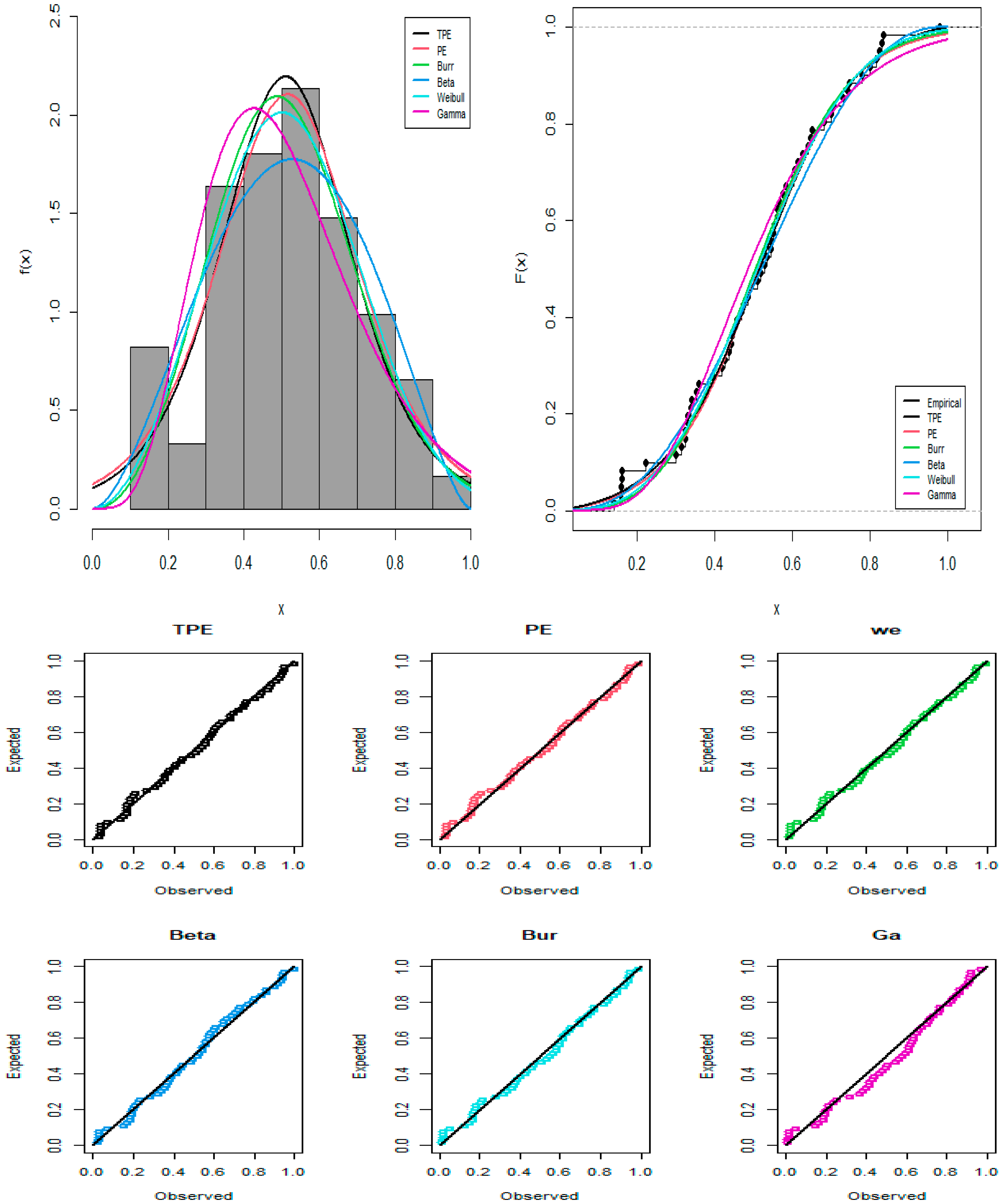
. Figure 5, Figure 6, and Figure 7, respectively, illustrate some graphical renderings of these datasets. These encompass histograms, kernel density estimates, violin plots, box plots, total time on test (TTT) plots, and quantile–quantile (QQ) plots. These figures show that all of the datasets have an increasing HRF. Also, the first and third datasets are slightly right-skewed, while the second dataset is left-skewed. The first and second datasets are almost symmetrical with no visible outliers, while the third dataset exhibits a non-normal distribution with no visible outliers. These characteristics can be handled by the TPE distribution as developed in the theoretical results.

Key statistical aspects are indicated by colors and symbols: In the violin plot, the green area indicates density, and the white dot is the median; in the box plot, the orange box represents the middle 50% of the data, the red dot is the mean, and the blue dots are data points. Pink and yellow are used in TTT and QQ charts to illustrate empirical versus theoretical behavior.

This comparative analysis rigorously evaluates the TPE model in relation to many rival models, including the Weibull (We), Beta, Gamma (Ga), Burr XII, and Perk (PE) distributions. The maximum likelihood method was utilized for parameter estimation and goodness-of-fit evaluation using the R programming language.

Table 15. Results of E₁ estimates with standard errors for dataset I.

Models	Est. of ($\mathit{\alpha }$)	SE ($\widehat{\mathit{\alpha }}$)	Est. of ($\mathit{\lambda }$)	SE ($\widehat{\mathit{\lambda }}$)
TPE	0.0151	0.0089	8.1242	1.0746
PE	0.0119	0.0065	8.6702	0.9542
Weibull	2.9501	0.3006	0.5764	0.0263
Gamma	5.8889	1.0332	0.0873	0.0159
Beta	2.7938	0.4879	2.6037	0.4519
Burr XII	3.1982	0.3025	6.5211	1.1239

,

Table 16. Results of E₁ estimates with standard errors for dataset II.

Models	Est. of ($\mathit{\alpha }$)	SE ($\widehat{\mathit{\alpha }}$)	Est. of ($\mathit{\lambda }$)	SE ($\widehat{\mathit{\lambda }}$)
TPE	0.0198	0.0087	8.2796	0.8375
PE	0.0167	0.0069	8.6951	0.7653
Weibull	2.6012	0.2098	0.5236	0.0202
Gamma	3.6911	0.4830	0.1270	0.0178
Beta	2.4124	0.3144	2.8296	0.3744
Burr XII	2.8016	0.2097	6.7692	0.9368

and

Table 17. Results of E₁ estimates with standard errors for dataset III.

Models	Est. of ($\mathit{\alpha }$)	SE ($\widehat{\mathit{\alpha }}$)	Est. of ($\mathit{\lambda }$)	SE ($\widehat{\mathit{\lambda }}$)
TPE	0.0157	0.0168	6.0768	1.9100
PE	0.0073	0.0062	7.8643	1.3028
Weibull	3.4129	0.5800	0.7156	0.0484
Gamma	9.6827	2.9062	0.0662	0.0204
Beta	2.1716	0.6681	1.0997	0.3055
Burr XII	3.7916	0.5926	4.2829	1.0505

present the results for parameter estimates and their corresponding standard errors. The findings from

Table 18. Results of goodness of-fit of the TPE model for dataset I.

Models	AIC	BIC	CAIC	HQIC	KS	p-Value
TPE	−25.327	−21.105	−25.120	−23.672	0.0519	0.9937
PE	−23.291	−19.069	−23.084	−21.637	0.0599	0.9714
Weibull	−25.273	−21.052	−25.066	−23.869	0.0591	0.9750
Gamma	−19.409	−15.188	−19.203	−17.755	0.0891	0.6843
Beta	−23.906	−19.684	−23.698	−22.251	0.0618	0.9628
Burr XII	−24.068	−19.847	−23.862	−22.414	0.0633	0.9545

,

Table 19. Results of goodness of-fit of the TPE model for dataset II.

Models	AIC	BIC	CAIC	HQIC	KS	p-Value
TPE	−49.274	−43.928	−49.158	−47.106	0.0542	0.9121
PE	−46.832	−41.487	−46.717	−44.665	0.0584	0.8594
Weibull	−38.695	−33.349	−38.579	−36.527	0.0832	0.4491
Gamma	−14.849	−9.503	−14.734	−12.682	0.1364	0.0374
Beta	−43.554	−38.209	−43.439	−41.387	0.091	0.3383
Burr XII	−33.474	−28.129	−33.359	−31.307	0.0884	0.3733

and

Table 20. Results of goodness of-fit of the TPE model for dataset III.

Models	AIC	BIC	CAIC	HQIC	K-S	p-Value
TPE	−4.4748	−2.3858	−3.8081	−4.0214	0.1204	0.9212
PE	−1.2453	0.8437	−0.5786	−0.7919	0.1359	0.8323
Weibull	−3.1874	−1.0984	−2.5207	−2.7340	0.1235	0.9059
Gamma	−4.2233	−2.1343	−3.5566	−3.7699	0.1309	0.8642
Beta	−4.3639	−2.2749	−3.6973	−3.9106	0.2119	0.3023
Burr XII	−3.0248	−0.9357	−2.3581	−2.5714	0.1262	0.8916

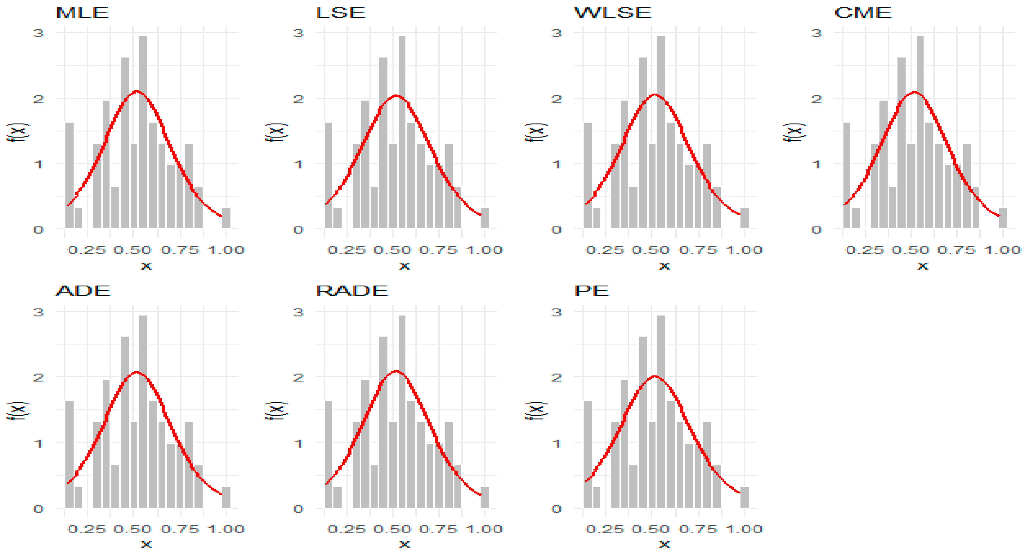
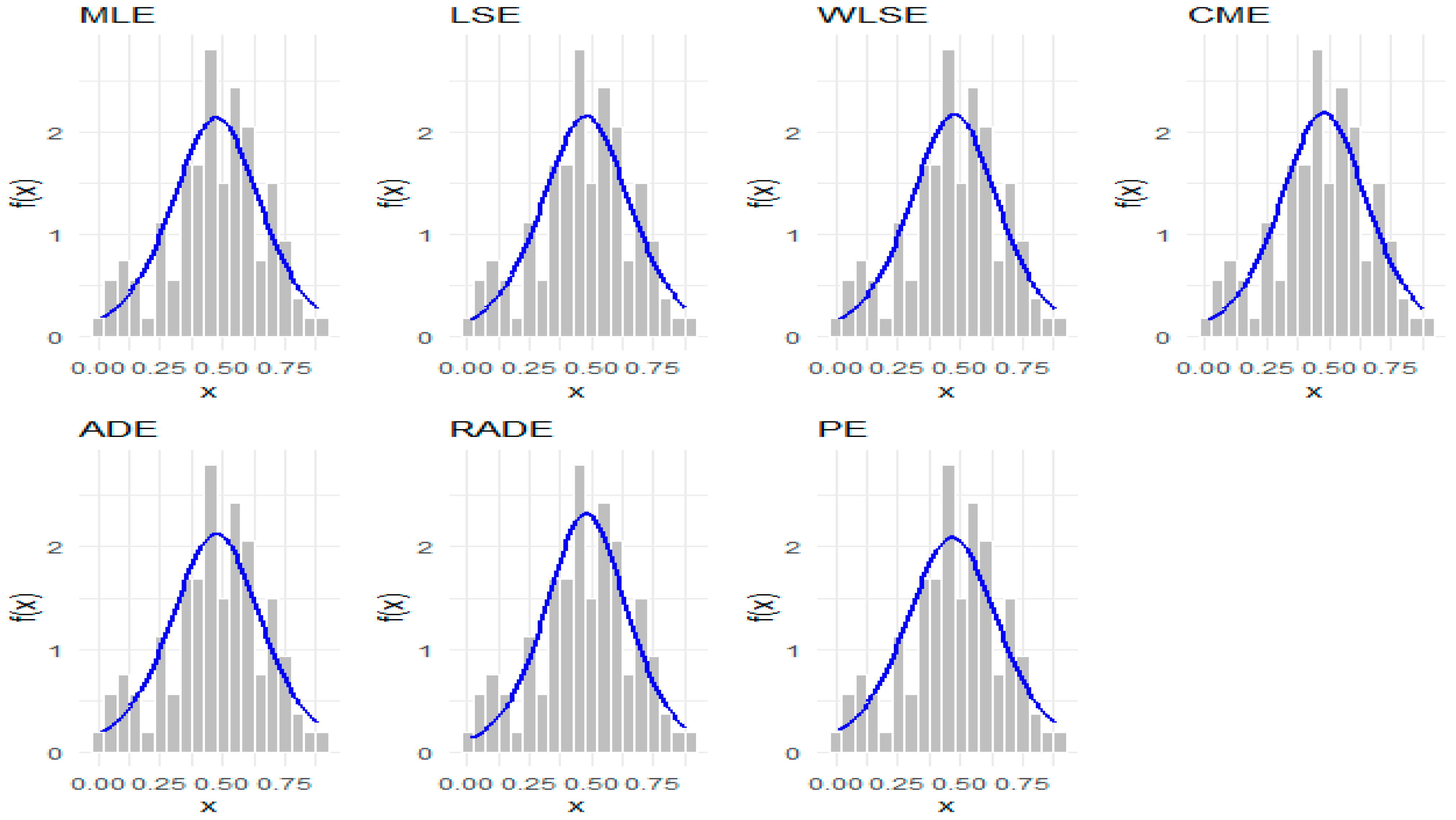
indicate that the TPE model demonstrates superior performance among all compared distributions, as indicated by it obtaining the lowest values in different goodness-of-fit metrics, including AIC, BIC, CAIC, HQIC, and K-S, as well as the greatest p-value. The estimated values for various estimation methods used on the TPE model for this dataset are displayed in

Table 21. Results of comparison between estimation methods of the TPE model for dataset I.

Methods	$\mathit{\alpha }$	$\mathit{\lambda }$	Measures of Adequacy
	Estimate	Estimate	K-S	p-Value
E1	0.0151	8.1242	0.0519	0.9937
E2	0.0177	7.8085	0.0451	0.9992
E3	0.0169	7.8952	0.0473	0.9982
E4	0.0155	8.0645	0.0509	0.9950
E5	0.0161	7.9969	0.0490	0.9970
E6	0.0157	8.0402	0.0503	0.9958
E7	0.0189	7.6839	0.0483	0.9976

,

Table 22. Results of comparison between estimation methods of the TPE model for dataset II.

Methods	$\mathit{\alpha }$	$\mathit{\lambda }$	Measures of Adequacy
	Estimate	Estimate	K-S	p-Value
E1	0.0198	8.2796	0.0542	0.9121
E2	53.9968	8.3468	0.0565	0.8842
E3	54.7575	8.4294	0.0564	0.8859
E4	57.9822	8.4929	0.0582	0.8612
E5	0.0202	8.2356	0.0536	0.9182
E6	78.2020	9.0905	0.0651	0.7554
E7	0.0232	8.0963	0.0518	0.9366

and

Table 23. Results of comparison between estimation methods of the TPE model for dataset III.

Methods	$\mathit{\alpha }$	$\mathit{\lambda }$	Measures of adequacy
	Estimate	Estimate	K-S	p-Value
E1	0.0157	6.0768	0.1204	0.9212
E2	0.0251	5.4643	0.1459	0.7629
E3	0.0148	6.3049	0.1328	0.8525
E4	0.0168	6.2306	0.1412	0.7964
E5	0.0294	4.7944	0.1436	0.7796
E6	0.0615	2.3159	0.1957	0.3973
E7	0.0133	6.3339	0.1231	0.9082

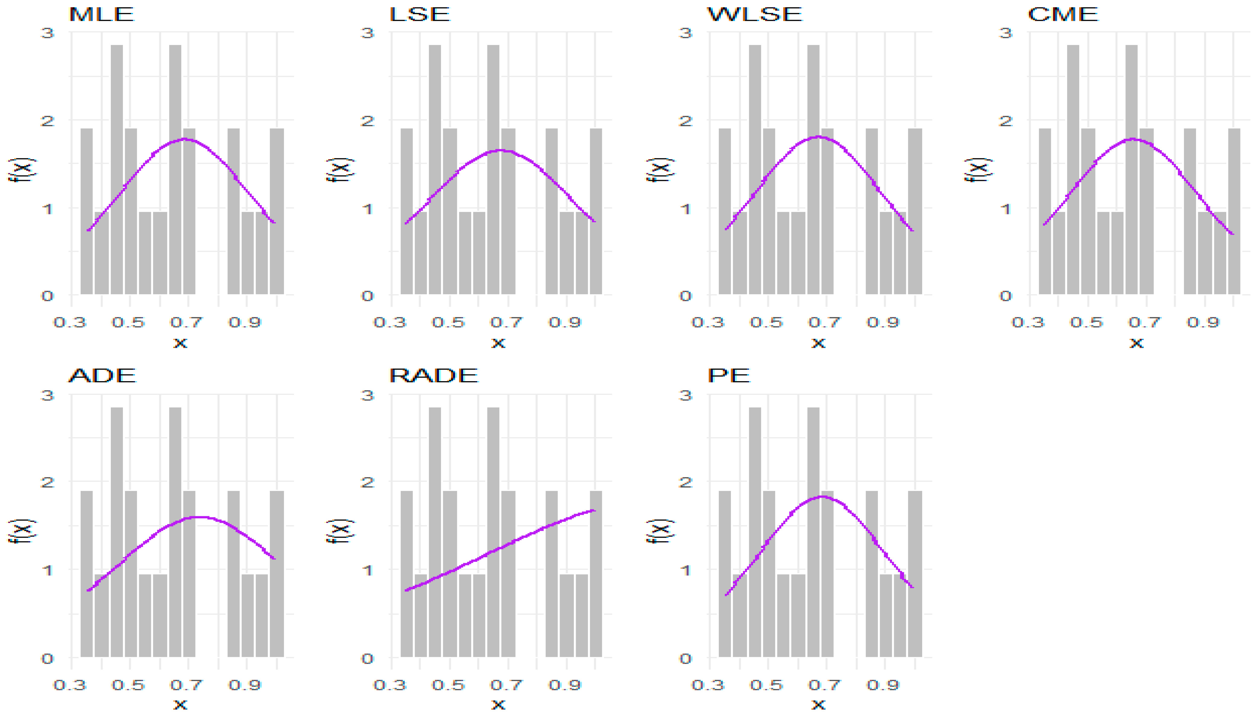
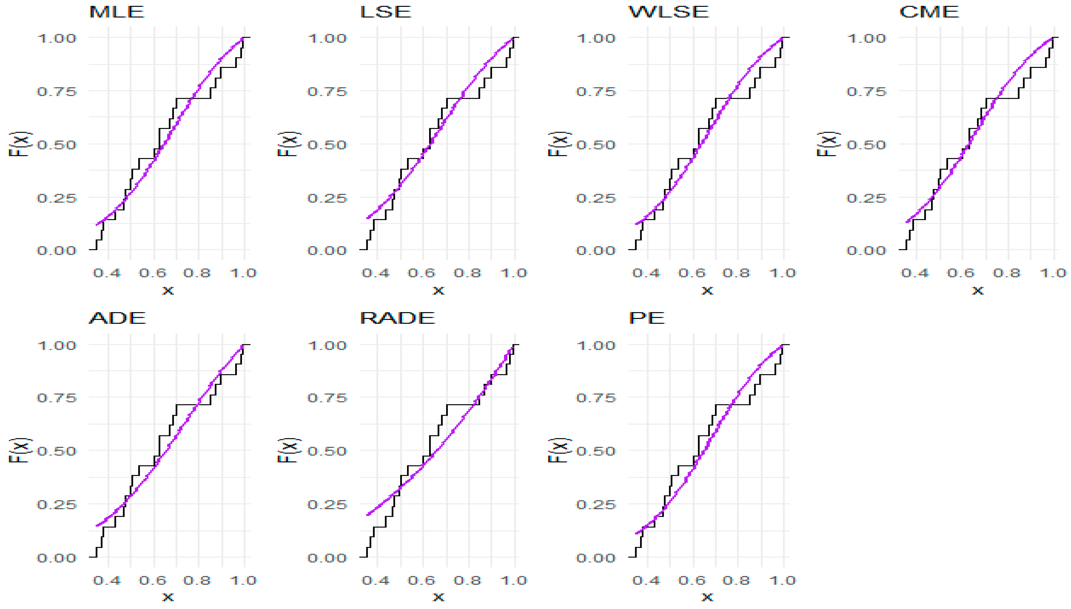
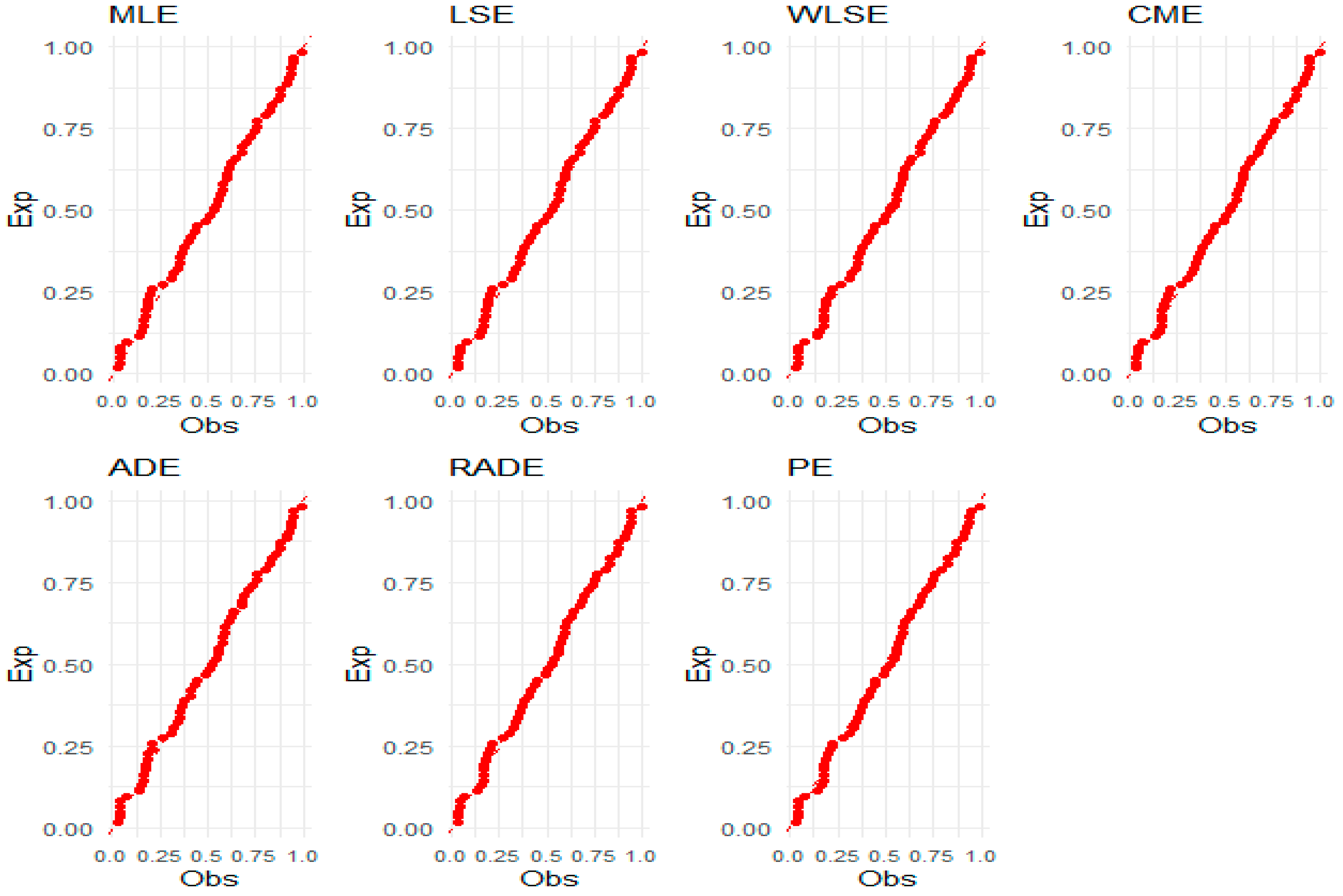
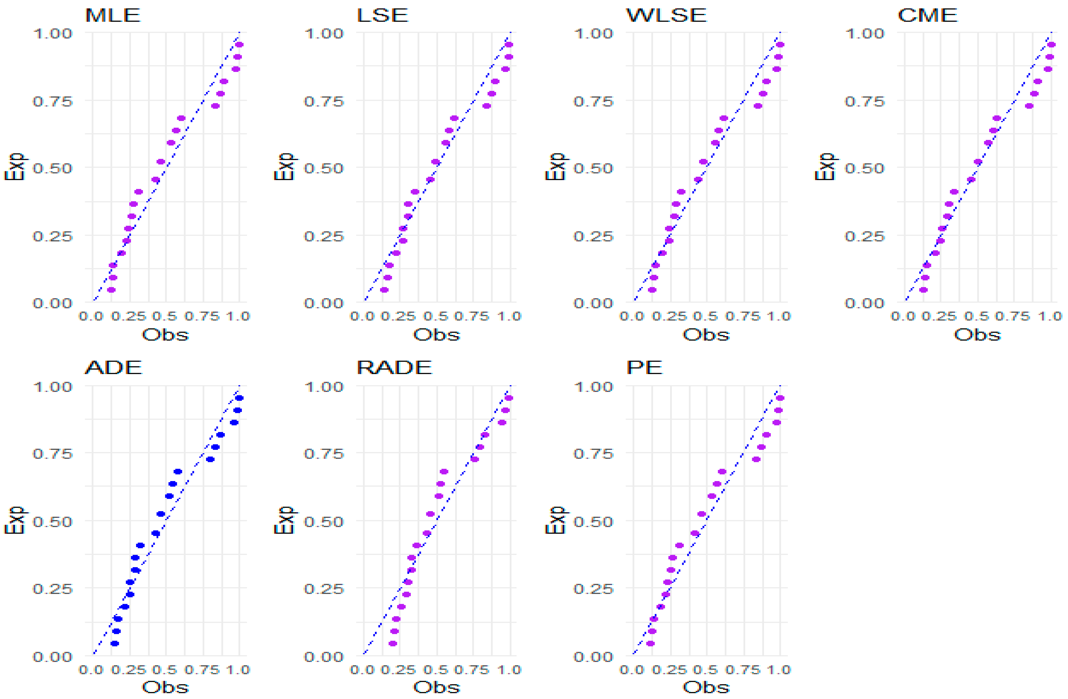
, which indicate that the E₂ method outperforms the others for the first dataset, the E₇ method excels for the second dataset, and the E₁ method leads for the third dataset, as evidenced by it obtaining the highest p-value. Additionally, Figure 8, Figure 9 and Figure 10 present graphical representations of densities, empirical cumulative distribution functions, and P–P plots for all competing models for the numerical data, facilitating a visual assessment of the models’ efficacy. Also, a visual comparison of the shape of the three datasets in the fitted PDFs, CDFs, and P–P plots is presented in Figure 11, Figure 12, Figure 13, Figure 14, Figure 15, Figure 16, Figure 17, Figure 18 and Figure 19.

8. Conclusions

This paper proposes the truncated Perk distribution for modeling data on the unit interval, which stems from an exploration of an appropriate transformation. The statistical features of the proposed model, including its quantile function, Rényi entropy, Tsallis entropy, order statistics, and moments, with some associated measures, were presented. The parameter estimators of the proposed distribution were determined using seven classical estimation techniques, including E₁, E₂, E₃, E₄, E₅, E₆, and E₇, with the R programming language. The efficacy of parameter estimate approaches was analyzed using limited samples through an extensive simulation study. We evaluated the efficacy of the estimates regarding their bias and mean squared error. This paper conducts a comparative analysis between the MLE method and Bayesian estimation to assess the performance of the proposed model. While the MLE method is known for its efficiency in large samples, Bayesian methods offer advantages when prior information is available or sample sizes are limited. Three empirical datasets and their comparative analyses, with varying distributions, are employed to visually elucidate the efficacy of the proposed distribution for data modeling. During the analytical development of the TPE distribution, several challenges arose due to the complex form of the density and its bounded support. Obtaining closed-form expressions for moments, entropies, and the moment generating function required advanced manipulations, including series expansions and variable transformations. The generalized binomial theorem was used to simplify moment derivations, while beta-type integral techniques were applied to obtain Rényi and Tsallis entropies. These steps ensured analytical tractability and reflect a novel methodological contribution to the study of bounded distributions.

Future research will consider an assessment of the stress–strength reliability model for the TPE distribution.