Article

Modified Two-Parameter Ridge Estimators for Enhanced Regression Performance in the Presence of Multicollinearity: Simulations and Medical Data Applications

by
Muteb Faraj Alharthi
1 and
Nadeem Akhtar
2,*
1
Department of Mathematics and Statistics, College of Science, Taif University, Taif 21944, Saudi Arabia
2
Government Degree College Achini Payan, Higher Education, Archives and Libraries Department, Peshawar 25000, Khyber Pakhtunkhwa, Pakistan
*
Author to whom correspondence should be addressed.
Axioms 2025, 14(7), 527; https://doi.org/10.3390/axioms14070527
Submission received: 2 June 2025 / Revised: 1 July 2025 / Accepted: 6 July 2025 / Published: 10 July 2025
(This article belongs to the Special Issue Applied Mathematics and Mathematical Modeling)

Abstract

Predictive regression models often face a common challenge known as multicollinearity. This phenomenon can distort the results, causing models to overfit and produce unreliable coefficient estimates. Ridge regression is a widely used approach that incorporates a regularization term to stabilize parameter estimates and improve the prediction accuracy. In this study, we introduce four newly modified ridge estimators, referred to as RIRE1, RIRE2, RIRE3, and RIRE4, that are aimed at tackling severe multicollinearity more effectively than ordinary least squares (OLS) and other existing estimators under both normal and non-normal error distributions. The ridge estimators are biased, so their efficiency cannot be judged by variance alone; instead, we use the mean squared error (MSE) to compare their performance. Each new estimator depends on two shrinkage parameters, k and d , making the theoretical analysis complex. To address this, we employ Monte Carlo simulations to rigorously evaluate and compare these new estimators with OLS and other existing ridge estimators. Our simulations show that the proposed estimators consistently minimize the MSE better than OLS and other ridge estimators, particularly in datasets with strong multicollinearity and large error variances. We further validate their practical value through applications using two real-world datasets, demonstrating both their robustness and theoretical alignment.

1. Introduction

Multicollinearity is a prevalent challenge in predictive modeling, occurring when input features exhibit high correlation, which results in unstable model estimates and reduced prediction accuracy.
The multiple linear regression model is a widely used statistical tool across disciplines, including business, environmental studies, industry, medicine, and social sciences. A crucial assumption of this model is the independence of explanatory variables. However, in practice, explanatory variables often exhibit moderate to strong linear relationships, leading to multicollinearity. This instability makes the coefficients less reliable. In a basic regression model, we have
y = X α + ϵ .
In Equation (1), y R n × 1 denotes the vector of observed responses, X R n × p represents the design matrix comprising the predictor variables, α R p × 1 is the vector of unknown regression coefficients, and ε R n × 1 is the vector of random errors.
The typical method for estimating these coefficients is the OLS method, which is represented in Equation (2) as follows:
α ^ O L S = X X 1 X y     a n d     C o v α ^ O L S = σ 2 X X 1 .
A key measure for detecting multicollinearity is the Condition Number (CN), which compares the largest ( λ m a x ) and smallest ( λ m i n ) eigenvalues of the matrix X X :
C N X = λ m a x λ m i n .
A high CN (e.g., greater than 30) suggests severe multicollinearity, which leads to unstable estimates of the regression coefficients. Another common diagnostic tool is the Variance Inflation Factor (VIF), which measures how much the variance of a regression coefficient is inflated due to multicollinearity. It is calculated for each predictor as in Equation (4).
V I F i = 1 1 R i 2 ,
where R i 2 is the coefficient of determination when the i t h predictor is regressed on all the others. A VIF greater than 10 indicates sever multicollinearity in the data. When multicollinearity exists, the matrix X X becomes close to singular, which makes OLS estimates less reliable. One effective solution is the ridge regression, a regularization technique that introduces a penalty term to mitigate overfitting [1]. In ref. [2], the authors modified new ridge estimator for severe multicollinear datasets. The shrinkage parameter, which controls the strength of regularization, was tuned simultaneously to find optimize the regression coefficients. The shrinkage parameter adjustment takes place during both the tuning and validation phases to achieve a balance between fitting the data well and avoiding overfitting.
  • A ridge estimator is defined as follows:
α ^ r i d g e = X X + k I 1 X y .
The k term, a small positive value known as the shrinkage or ridge parameter, is used to improve the numerical stability of the regression model. Additionally, I is the identity matrix, which is controlled by the ridge parameter k. This technique effectively shrinks the coefficients, which, in turn, helps reduce the variance or minimize the MSE. A key strength of the ridge parameter k is its simplicity and computational efficiency, especially when the model includes fewer independent variables. However, the performance of ridge estimators is highly influenced by the choice of k, which is typically determined through cross-validation. There are scenarios where a single regularization parameter may not be sufficient, especially in complex models. This is where two-parameter ridge estimators come into play, offering advantages over the traditional ridge estimator is widely used to handle multicollinearity. For example, ref. [3] examined coefficient testing under ridge models, while ref. [4] proposed a new ridge-type estimator with improved performance.
However, ref. [5] introduced the two-parameter ridge or shrinkage estimator, which adds another scale parameter, d , to adjust the penalty term, as in Equation (6).
α ^ ( d , k ) = d X X + k I 1 X y ,
where
d ^ = X y X X + k I 1 X y X y X X + k I 1 X X X X + k I 1 X y .
This approach allows for more flexibility, making it better suited for handling multicollinearity in complex cases. If d = 1   a n d   k = 0 , Equation (6) reverts to the standard OLS estimator. The authors in [6] improved the two-parameter ridge regression estimator for the multicollinearity dataset and compared their estimators with others based on the MSE.
While ref. [7] introduced a generalized ridge estimator as a comprehensive solution for handling severe multicollinearity, ref. [8] introduced three shrinkage estimators based on averages for severe multicollinear data. Ref. [9] developed the bias–variance trade-off by incorporating data-specific tuning parameters, offering a more tailored approach to ridge regression.
Theoretical improvements have focused on utilizing higher-order eigenvalue terms to improve ridge regression techniques. Ref. [10] developed new ridge estimators to effectively reduce the effect of multicollinearity from the data. Ref. [11] further highlighted and improved the shrinkage parameters in practical applications of ridge regression to address multicollinearity, making it an essential tool in regression analysis. While refs. [12,13] expanded the scope of ridge estimators to handle severe multicollinearity datasets in fields such as genetics, environmental studies, and econometrics, ref. [14] proposed ridge estimators based on rank, a method particularly useful for analyzing complex multicollinearity genetic data.
Extensive research has been conducted on estimating the ridge or shrinkage parameters in linear regression models. Ref. [15] innovated two-parameter estimators of complex multicollinear data to improve the accuracy of the Almon distributed-lag model. Ref. [16] developed ridge estimators to enhance the accuracy of linear regression models and compared these estimators with OLS and other established estimators based on the MSE. More recently, ref. [17] used bootstrap–quantile and improved ridge estimators for linear regression, while ref. [18] introduced six new two-parameter ridge estimators to address multicollinearity challenges and compared these modified estimators with other established estimators based on the MSE. The authors in both [19,20] further introduced two-parameter ridge estimators to more effectively handle data with high multicollinearity, compared to other existing estimators.
The literature clearly shows that no single ridge estimator performs well across all multicollinearity scenarios. To deal with this issue, many researchers have proposed modifications to improve the estimator performance under severe multicollinearity. In this study, we propose four new ridge-type estimators, denoted as RIRE1, RIRE2, RIRE3, and RIRE4, that demonstrate better performance in simulation studies across different conditions such as sample sizes, number of predictors, error variances, and correlation structures. These estimators outperform the OLS and other existing shrinkage methods, maintaining robust efficiency under both normal and non-normal distributions, particularly when datasets have severe multicollinearity. The remainder of the paper is organized as follows: Section 2 presents the statistical methodology for ridge estimators, including a review of existing estimators and the introduction of our four newly modified estimators. Section 3 describes the Monte Carlo simulations conducted to assess the performance of these estimators under various conditions. In Section 4, the proposed estimators are applied to the analysis of two real-world datasets to demonstrate their practical utility. Finally, Section 5 offers concluding remarks and summarizes the key findings of the study.

2. Methodology

Ridge regression is a supervised learning method that adds a penalty term to the regression equation in order to reduce multicollinearity. This section provides the mathematical foundation for existing ridge estimators and the newly proposed modified estimator for ridge regression models.
To simplify the regression model in Equation (1), we can reformulate it into its canonical form as
y = U β + ϵ ,
where U = X Q is the transformed design matrix, β is the parameter vector in the canonical space, and ϵ represents the noise, as before. The matrix Q is orthogonal, derived from the eigenvectors of X X , and satisfies Q Q = I p . This transformation aligns the design matrix U with the principal components of X , simplifying the regression problem.
Additionally, we define
Λ = Q X X Q ,
where Λ is a diagonal matrix containing the eigenvalues λ 1 , λ 2 , , λ p arranged in ascending order. The relationship between the original parameters and the canonical parameters is expressed as β = Q α , which enables the model to operate in the canonical space.
In this form, the OLS estimator becomes
β ^ = Λ 1 U y ,
where Λ 1 scales U y by the inverse eigenvalues. However, small eigenvalues can cause instability in the OLS solution. Ridge regression mitigates this by introducing a regularization parameter k > 0 , modifying the estimator to be
β ^ k = Λ + k I p 1 U y ,
which adds k to the diagonal elements of Λ, stabilizing the solution by reducing the influence of small eigenvalues.
A generalized two-parameter ridge regression estimator extends this idea, taking the form
β ^ ( d , k ) = d Λ + k I p 1 U y ,
where d adjusts the intensity of shrinkage. This added flexibility allows for better control over the trade-off between bias and variance, catering to various modeling requirements.

2.1. Existing Ridge-Type Estimators

In this part, some existing estimators are discussed and reviewed. Hoerl and Kennard in [1] developed the first ridge estimator, commonly known as the HK estimator, and its mathematical formulation is given as
k ^ H K = σ ^ 2 β ^ M a x 2   with   β M a x = m a x ( β 1 ,   β 2 ,   , β p ) .
The authors in [8] explored three ridge estimators designed to address multicollinearity in data using averaging techniques. These are the Arithmetic Mean (KAM), the Geometric Mean (KGM), and the Median (KMed). They are mathematically expressed as
k ^ A M = 1 p i = 1 p σ ^ 2 β ^ i 2 , k ^ G M = σ ^ 2 i = 1 p β ^ i 2 1 p , k ^ M e d = M e d σ ^ 2 β ^ i 2 .
Ref. [21] introduced an eigenvalue-based estimator, known as the KMS estimator, to effectively handle multicollinearity. Its mathematical expression is given as
k ^ K M S = λ max i = 1 p β ^ i σ ^ 2 β ^ M a x 2 .
Similarly, a two-parameter ridge estimator, referred to as the TK estimator, was established by [6], with the optimal values for d ^ o p t and k ^ o p t derived as follows:
d ^ o p t = i = 1 p β ^ i 2 λ i λ i + k i = 1 p β ^ 2 λ i + γ ^ i 2 λ i 2 λ i + k 2 ,
k ^ o p t = d ^ o p t i = 1 p σ ^ 2 λ i + d ^ o p t 1   i = 1 p β ^ i 2 λ i 2 i = 1 p β ^ i 2 λ i .
Ref. [22] developed three estimators for multicollinearity data, denoted as MPR1, MPR2, and MPR3. Their mathematical expressions are given below:
k ^ M P R 1 * = i = 1 p k i * p     , k ^ M P R 2 * = i = 1 p k i * 1 p     , k ^ M P R 3 * = p i = 1 p 1 k i *       .
In these formulations, the adjusted ridge parameter for the i t h predictor is computed as
k i * = ω i k ^ o p t ,
where β i is a weight defined by the ratio of the eigenvalue λ i to the absolute value of the corresponding coefficient estimate β i :
ω i = λ i β i .
From the well-established ridge-type estimators available, we selected the estimators HK, KAM, KGM, KMed, KMS, TK, MPR1, MPR2, MPR3, and OLS to be compared with our four modified estimators using Monte Carlo simulations based on the MSE.

2.2. New Ridge-Type Estimators

The newly proposed estimators, referred to as RIRE1, RIRE2, RIRE3, and RIRE4, effectively address various multicollinearity conditions. For these estimators, the k ^ i values ( i = 1 , 2 , 3 , 4 ) are presented below:
k ^ 1 = log 1 + i = 1 p λ i β ^ i σ ^ 2 ,
In this estimator, the logarithmic function imposes a nonlinear growth constraint on the penalization term. By summing λ i β ^ i over p , this estimator accumulates the contribution of each variable to multicollinearity.
k ^ 2 = i = 1 p λ i 2 β ^ i p max β ^ i ,
Squaring the eigenvalues in this estimator increases the weight of highly collinear directions. Normalizing by the maximum coefficient ensures that the penalty strength does not disproportionately increase due to one dominant variable. Thus, RIRE2 enforces balanced shrinkage that is tailored to both the multicollinearity severity and the variable scale.
k ^ 3 = i = 1 p λ i β ^ i 2 p   σ ^ 2 ,
The RIRE3 estimator captures the squared contribution of eigenvalue-weighted coefficients, scaled by residual variance, effectively linking penalization strength to the overall signal-to-noise ratio in the presence of multicollinearity.
k ^ 4 = i = 1 p λ i 3 β ^ i 2 p i = 1 p λ i β ^ i 2 .
RIRE4 introduces higher-order penalization sensitivity by cubing the eigenvalues and squaring the coefficients, allowing it to react more forcefully to severe collinearity. The denominator acts as a normalization factor, stabilizing the shrinkage magnitude. This estimator is particularly effective when a subset of predictors exhibits extremely high multicollinearity.
Equations (19)–(22) are used to optimize the k ^ -values, while Equation (7) is utilized to compute d ^ .

2.3. The Performance of Estimators Based on the MSE Criterion

We assessed and compared the performance of our proposed modified estimators with OLS and other existing estimators based on the MSE criterion. The MSE has been applied in various studies such as in [23,24,25,26,27,28] to evaluate the accuracy of estimators. The MSE can be calculated as
M S E β ^ = E ( β ^ β ) β ^ β
= 1 p i = 1 p ( β ^ β ) 2 .
Since it is challenging to compare Equations (23) and (24) theoretically, we will, instead, analyze their performance through Monte Carlo simulations in the next section.

3. Computational Analysis Using Monte Carlo Simulation

Equation (25) is used for generating predictors as seen in previous research studies [26,27,28].
x i j = 1 ρ 2 U j i + ρ U j , p + 1 ,   i = 1,2 , , p ;   j = 1,2 , , n .
The correlation ( ρ ) between predictors was varied across values of 0.50, 0.70, 0.88 ,   0.94 ,   0.98 ,   and   0.999 to examine different multicollinearity scenarios. Independent samples ( U j i ) were drawn from a standard normal distribution, with sample sizes ( n = 20 ,   50 ,   100 ) and predictor counts ( p = 4 ,   10 ) used to evaluate model robustness. The response variable ( y i ) was generated using the following model:
y i = β 0 + i = 1 p j = 1 n β i x i j + ϵ j ,
where β 0 is the intercept (set to zero), β i is the regression coefficient, and ϵ j is the error term with variance σ 2 analyzed at levels 0. 4, 1, 4, and 8. Furthermore, to examine the impact of non-normal errors, we generated error terms from a t-distribution with 2 degrees of freedom ( t ( v = 2 ) ) and an F-distribution with 6 and 12 degrees of freedom (F (6,12)).
To calculate the MSE of the estimators, Algorithm 1 was used, as detailed below.
Algorithm 1 Step-By-Step Procedure for MSE
  • Standardize the matrix of independent variables using Equation (25), then compute eigenvalues λ 1 , , λ p and eigenvectors e 1 , , e p of X′X. Determine regression coefficients β in canonical form as β   = e m a x   P ,   where P = e 1 , , e p and e m a x corresponds to the maximum eigenvalue.
  • Generate random error terms from N 0 , σ 2 , ( t ( v = 2 ) ) and F (6,12). Compute dependent variable values using Equation (12).
  • Calculate OLS and ridge regression estimates using their expressions. Repeat for ( N ) Monte Carlo iterations and calculate the MSE for all estimators using Equation (27):
M S E β ^ = 1 N j N i = 1 p ( β ^ j i β ) 2 .
Simulations with N = 10,000 were performed in R to evaluate the MSE across varying values of ρ , n , and p . Table A1, Table A2, Table A3 and Table A4 in Appendix A present the MSEs for the proposed and existing estimators under these conditions. All analyses were conducted using R version 4.1.0. Detailed analysis follows in the next section.

Discussion and Analysis

The comparison of estimators in Table A1 and Table A2 illustrates how their performance, as measured by the MSE criterion, varies under different conditions, including variations in the sample size ( n ) , number of predictors (p), predictor correlations ( ρ ) , and error variance σ 2 generated from N 0 , σ 2 . Table A3 and Table A4 present the MSEs of different estimators when the error term is generated from a standardized t-distribution with 2 degrees of freedom (t2) and an F-distribution with 6 and 12 degrees of freedom. This heavy-tailed error distribution introduces significant deviations from normality, challenging the robustness of classical estimators.
Here are some resulting remarks from the analysis:
i.
Effect of Sample Size ( n ): A small sample size ( n = 20 ) exacerbated the limitations of the OLS and some classical ridge estimators, particularly under high correlations ( ρ > 0.9 ) and large predictor counts ( p = 10 ) . For instance, OLS demonstrated very high MSEs in these cases, reflecting its instability in multicollinearity. Conversely, as the sample size increased ( n = 50   o r   n = 100 ) , the MSE of all the estimators decreased, with the HK estimator showing improved performance. The KAM, KGM, and KMed estimators improved their performance in large sample sizes. For n = 20 , OLS showed significant variability in the error variance, especially as the correlation increased from 0.50   t o   0.70 . As the sample size increased ( n = 50 and n = 100 ), the estimates stabilized, with OLS providing more consistent results. Higher error variances (σ2 = 0.98 ) exacerbated this sensitivity, particularly in smaller samples. Estimators such as MPRs and RIREs showed less variability and became more reliable as the sample size increased. Notably, RIRE2, RIRE4, and MTPR estimators maintained low MSEs even in small-sample scenarios, suggesting their robustness to sample size variations.
ii.
Effect of Predictors ( p ): The number of predictors significantly affected the estimators’ performance. When p is small ( p = 4 ) , classical ridge estimators such as HK, KAM, KGM, and KMed estimators performed relatively well under moderate multicollinearity ( ρ = 0.88   o r   0.94 ) . However, as p increased to 10 , their MSE increased substantially, especially in high multicollinearity settings. This trend was more pronounced in OLS, which struggled to accommodate a higher predictor count. By contrast, RIRE2, RIRE4, and MPR variants exhibited remarkable scalability, maintaining low MSEs regardless of the predictor count.
iii.
Effect of Correlations ( ρ ): High correlations among the predictors ( ρ = 0.98   o r   0.999 ) dramatically increased the MSE for OLS and classical ridge estimators. For example, the MSE of HK escalated in these conditions, particularly in small sample sizes and larger predictor settings. RIRE estimators and MTPR variants, however, showed resilience to extreme correlations, consistently achieving the lowest MSE across all scenarios.
iv.
Effect of Error Variance  σ 2 : The ridge estimators (e.g., HK and KMS) were particularly sensitive to a high error variance ( σ 2 ), with their performance deteriorating in settings where both ρ and p were high. Our RIRE estimators demonstrated relative stability, maintaining lower MSEs under increasing error variances. MPR estimators also performed well in managing the effects of a higher error variance, making them suitable for noisy data.
v.
To assess the effect of non-normal error terms, errors were simulated from a heavy-tailed t-distribution with 2 degrees of freedom, which introduces significant departures from normality by allowing extreme values or outliers. Under these challenging conditions, classical estimators such as the OLS and conventional ridge-based methods (HK, KAM, KGM, KMed, KMS, TK, MPR1–MPR3) exhibited notably high mean squared errors (MSEs), especially at high correlation levels ( ρ close to 1). In contrast, the proposed modified ridge estimators (RIRE1 to RIRE4) showed marked resilience to the heavy-tailed noise structure. Their MSEs remained consistently low across different sample sizes and predictor dimensions, indicating enhanced robustness against outliers and extreme error values inherent to t2-distributed noise. The robustness is particularly important in practical scenarios where normality assumptions are violated and error distributions have heavy tails. Among the RIRE estimators, some estimators (RIRE2 and RIRE4) performed better, suggesting that their specific modifications effectively mitigate the influence of large error fluctuations. These results highlight the advantage of the new estimators in maintaining accuracy and stability in regression models affected by non-normal, heavy-tailed error distributions.
vi.
The findings from Table A3 indicate that the new RIRE estimators provide improved accuracy and stability compared with classical and existing methods in regression models with t2-distributed errors.
vii.
Table A4 show the MSEs when error terms follow a standardized F-distribution with (6, 12) degrees of freedom, representing heavy-tailed, non-normal errors. The modified ridge estimators (RIRE1–RIRE4) consistently outperformed OLS and other existing methods (HK, KAM, KGM, KMed, KMS, TK, MPR1–MPR3), especially at high correlations ( ρ ). Among them, RIRE3 and RIRE4 achieved the lowest MSEs, demonstrating superior robustness and accuracy under this complex error structure. This highlights the advantage of RIRE estimators in handling heavy-tailed, asymmetric noise effectively.
These results highlight that no single estimator performs optimally under all conditions. However, our modified estimators RIRE2 and RIRE4 consistently outperformed others when compared with OLS and other existing estimators in scenarios involving small samples, large predictors, high correlations, and high error variances. The other ridge estimators, such as HK, were effective under moderate conditions; however, they failed to handle extreme multicollinearity or challenging settings involving many predictors and small samples. OLS remained unsuitable for multicollinearity, especially when ρ > 0.90 .
The summary table (Table 1) was created based on the simulation results from Table A1, Table A2, Table A3 and Table A4. The proposed RIRE estimators demonstrated strong performance across a wide range of conditions, consistently outperforming other methods. In particular, RIRE3 and RIRE4 performed the best in 88 out of 120 cases, excelling in scenarios with varying sample sizes, error variances, and dimensions. RIRE2 also showed strength in nine scenarios, particularly at high error variances. Overall, our RIREs were the top choice in 97 out of 120 situations, proving their reliability and adaptability compared with alternatives such as MPR1 and MPR3, which performed well only in specific contexts.

4. Real-Life Applications

In this section, we utilize the newly modified proposed and competing estimators on three real-life applications. The first dataset is the Updated Longley (1959–2005), sourced from the Department of Labor, the Bureau of Statistics, and the Defense Manpower Data Center, Gujrati’s Basic Econometrics [29], and Mental Health and Digital Behavior (2020–2024). The second set of data is the Hospital Manpower dataset used in [17]. The third dataset is the Body Fat Dataset [30], which contains body composition measurements and is publicly available online. These datasets exhibit high multicollinearity and are recognized benchmarks for ridge regression analysis.

4.1. Practical Application of the Longley Dataset

The dataset consists of 47 observations spanning from 1959 to 2005, with a total of six variables:  y , X 1 , X 2 , X 3 , X 4 , and   X 5 . Thus, the regression model can be written as
y = β 0 + β 1 X 1 + β 2 X 2 + β 3 X 3 + β 4 X 4 + β 5 X 5 + ϵ ,
where y is the dependent variable, X 1   to   X 5 are the independent variables, β 0 is the intercept, β 1   to   β 5 are the coefficients for each independent variable, and ϵ is the error term.
To check for multicollinearity in the dataset, we looked at key indicators: eigenvalues, the CN, the VIF, and the heatmap display. These help in understanding how much the independent variables are related to each other and whether that could cause issues in our analysis. The eigenvalues of the dataset are: λ 1 4.278 , λ 2 0.714 , λ 3 0.113 , λ 4 0.00831 , and   λ 5 0.00832 .
We used Equation (3) to calculate the CN as follows:
C N = λ m a x λ m i n = 4.278 0.00831 514.94
The CN for the dataset is about 514.94, which points to a significant amount of multicollinearity. Such a high CN suggests that the independent variables are strongly correlated to each other.
Equation (4) was utilized to calculate the VIFs for each predictor X i .   R i 2 is the R-squared value from regressing X i on all the other predictors in the model. However, R i 2 can be approximated using the inverse of the correlation matrix of the dataset. The diagonal elements of the inverse of the correlation matrix represent 1 ( 1 R i 2 ) for each predictor. Therefore, the VIFs for the variables are as follows: X 1 (52.90), X 2 (79.94), X 3 (35.94), X 4 (4.18), and X 5 (4.81). High VIF values indicate multicollinearity, with a VIF greater than 10 suggesting significant correlation among the predictors. In this analysis, X 1 , X 2 , and X 3 showed high multicollinearity, while X 4 and X 5 had lower VIFs, indicating that they are less correlated with the other predictors.
Furthermore, in Figure 1, the heatmap shows that X 1 , X 2 , and X 5 are strongly related, meaning that they share a lot of the same information. In particular, X 1 is highly correlated with X 2 (0.97) and X 5 (0.99), which suggests that these variables move together. On the other hand, X 4 has a strong negative relationship with X 1 (−0.87) and X 5 (−0.87), indicating that as one increases, the other tends to decrease. This level of correlation could cause issues in regression analysis by making it harder to determine the unique effect of each variable. To remove the effect of severe multicollinearity, we used ridge regression, both with our proposed newly modified estimators and existing estimators.
The analysis of this real dataset validates the simulation results, confirming that our modified estimators (RIREs) performed better than other existing estimators, as shown in Table 2. Figure 2 shows that MPR1, RIRE2, and RIRE3 had the lowest MSEs, indicating the best overall estimator performance.

Comparison of the Estimators Based on Confidence Interval

The 99% confidence interval (C.I.) for each coefficient is calculated using the following formula: For each coefficient β ^ i (for i = 0 , 1 , 2 , , 5 ), C . I = β ^ i ± Z α 2 × S E , where Z α 2 is the critical value for a 99% C.I (2.576), and S E ( β ^ i ) is the standard error of the coefficients, which can be calculated from the MSE and the number of observations. For each estimator, we used the MSE provided to calculate the standard error for each coefficient.
The standard error can be computed using the formula
S E = M S E n , where n = 47 is the number of observations. We denoted L ( β i ) and U ( β i ) as the lower and upper bounds of the C.I, respectively.
From Table 3 and based on the provided confidence intervals, we see that RIRE4 had the narrowest intervals across most of the coefficients, particularly for β 0 ,   β 1 ,   a n d   β 5 , suggesting it as the most precise estimator. RIRE1 and RIRE2 also showed relatively narrow intervals but not as consistently as RIRE4. Thus, RIRE4 appears to be the best estimator, as it had the smallest range between the lower and upper bounds for most of the coefficients.

4.2. Hospital Manpower Data

This dataset contains 17 observations with five predictors: X 1 (monthly man-hours; Load), X 2 (monthly X-ray exposures; Xray), X 3 (occupied bed days; BedDays), X 4 (population in thousands; AreaPop), and X 5 (average patient stay; Stay). The dependent variable y represents the average daily patient load (Hours). The linear model is given as
y = β 0 + i = 1 5 β i X i + ϵ
To assess multicollinearity, the CN, VIF, and heatmap were used. The CN of about 278.87 far exceeds the common threshold of 30, indicating severe multicollinearity. The VIF values were ( X 1 (8.189), X 2 (7929.5), X 3 (4.083), X 4 (8504.7), and X 5 (19.75). Since values above 5 (or sometimes 10) indicate problematic multicollinearity, several variables here exceed that threshold. This, along with the very high CN, suggests strong inter-variable dependencies that could significantly affect the analysis.
It is also clear from Figure 3 that strong positive correlations among most hospital manpower variables were observed, except for moderate correlations involving X 3 , indicating potential multicollinearity issues in the dataset.
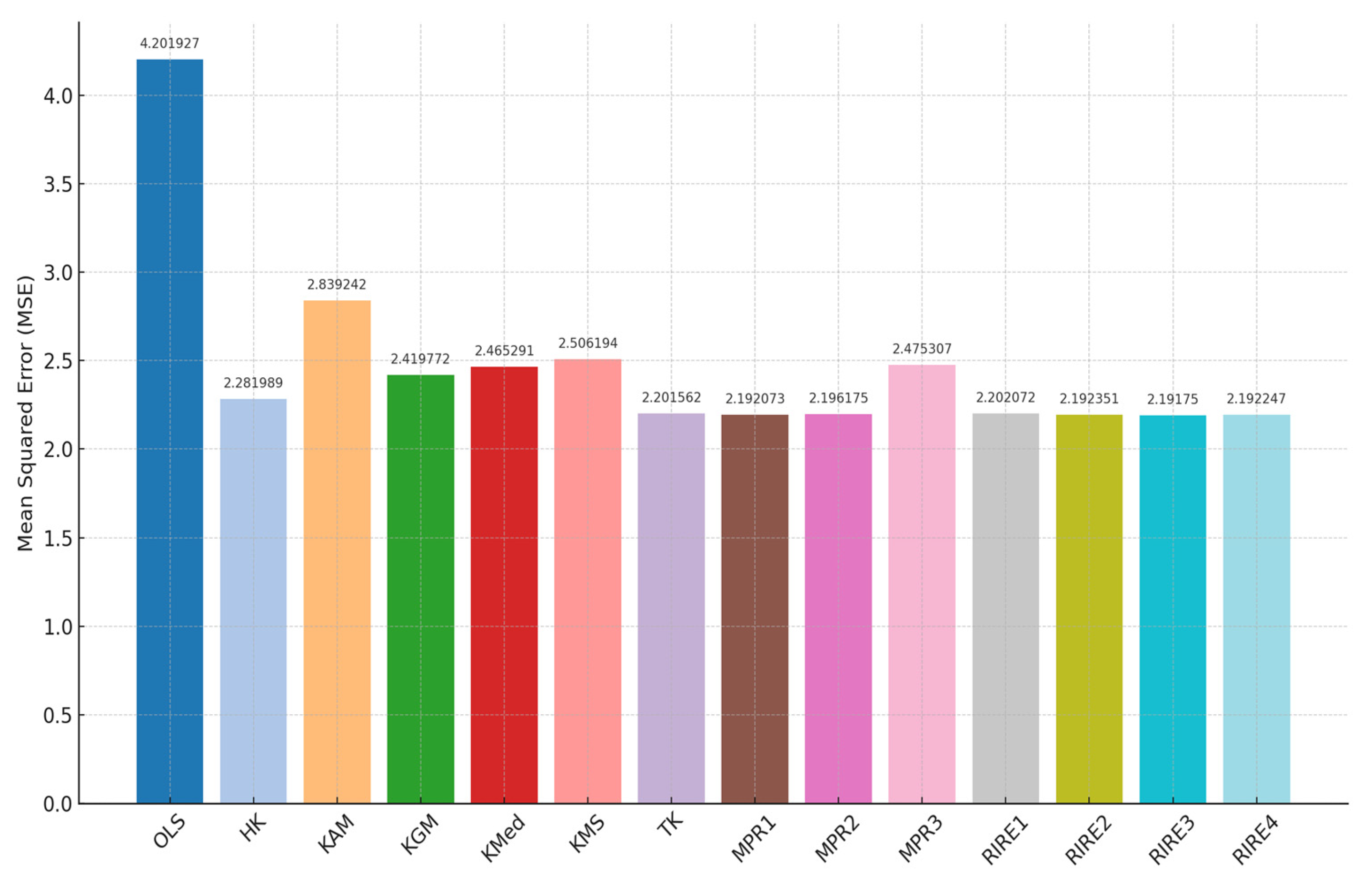
Table 4 shows that the newly proposed RIRE1–RIRE4 estimators consistently achieved the minimum MSE (2.19175–2.202072), outperforming OLS (4.201927) and the other existing methods. This indicates that the new proposed RIRE estimators provide better prediction accuracy on the Hospital Manpower data based on the MSE criterion. Figure 4 confirms that RIRE3, MPR1, and RIRE2 offer the most accurate estimates with minimal MSEs, while OLS demonstrates the least efficiency.

Comparisons of Estimator Coefficients Based on the 99% C.I for the Hospital Manpower Data

To calculate the 99% C.I. for the Hospital Manpower data regression model, we followed the same steps as above, ensuring correct application of formulas for the SE and the confidence intervals for n = 17 .
Table 5 presents the confidence intervals (C.I.) for the coefficients of several estimators applied to the Hospital Manpower dataset. The RIRE estimators outperformed the existing methods in terms of providing more consistent and narrower confidence intervals, particularly for coefficients like β 3 and β 4 . RIRE1 offered substantial improvements over OLS, with tighter intervals for most coefficients, especially β 1 and β 4 . RIRE2 showed better precision for β 3 , with narrower intervals than OLS, HK, and MPR1, although it still had wider intervals compared with KMS for certain coefficients. RIRE3 delivered significant improvements over OLS and TK, offering narrower and more stable intervals for several coefficients, especially for β 3 and β 4 . RIRE4 provided the most balanced results, with narrower intervals for β 1 , β 3 , and β 5 , outperforming traditional estimators (MPR2 and MPR3) in terms of precision. Overall, the RIREs produced more reliable and precise estimates compared with traditional methods, especially when dealing with multicollinearity issues in the dataset.

4.3. Body Fat Dataset

This dataset contains body composition and anthropometric data for 252 individuals, including variables like BODYFAT (y), DENSITY (X1), AGE (X2), WEIGHT (X3), HEIGHT (X4), ADIPOSITY (X5), and various circumferences (e.g., NECK (X6), CHEST (X7), ABDOMEN (X8), etc.). It is useful for analyzing the relationship between body fat and physical attributes. A regression model is given below:
y = β 0 + i = 1 15 β i X i + ϵ
Multicollinearity was assessed using CN, eigenvalues, VIF, and heatmap display. The results indicated severe multicollinearity, with a CN of 1234.89 (well above the threshold of 30) and VIF values between 2.31 and 62.63. Figure 5 suggests potential multicollinearity, particularly between variables such as weight, adiposity, and abdominal circumference, which exhibit very high correlations and could lead to issues in predictive modeling or regression analysis.
To address the issue of multicollinearity, we use our proposed and existing estimators to enhance model stability and to reduce the multicollinearity effects. Table 6 shows that the estimation in this third dataset aligns with the simulation results, where the proposed estimator RIRE3 achieved the minimum MSE compared with OLS and other existing ridge estimators.

5. Conclusions

This study presented four new modified ridge regression estimators, referred to as RIRE1, RIRE2, RIRE3, and RIRE4, which were designed to enhance precision in estimations when modeling multicollinear data. The adaptive characteristics of these estimators provided a versatile method for regularization, rendering them appropriate for contemporary predictive modeling challenges. The analysis highlighted the impressive performance of our newly modified RIRE estimators, especially RIRE2, RIRE3, and RIRE4, as they effectively handled challenging scenarios such as small sample sizes, severe multicollinearity, and large error variances compared with OLS and other existing estimators under both normal and non-normal error distributions. Our new estimators achieved the lowest MSE in both simulations and real-world dataset analyses, confirming their reliability and practical usefulness, which offer a clear advantage over other ridge regression estimators.
Future research could focus on adapting RIRE estimators for high-dimensional data and testing their effectiveness on a wider range of real-world datasets. This exploration would offer valuable insights into their potential for handling complex data structures.

Author Contributions

Conceptualization, M.F.A. and N.A.; methodology, M.F.A. and N.A.; software, M.F.A. and N.A.; validation, M.F.A. and N.A.; formal analysis, M.F.A. and N.A.; investigation, M.F.A. and N.A.; resources, M.F.A. and N.A.; data curation, M.F.A. and N.A.; writing—original draft preparation, M.F.A. and N.A.; writing—review and editing, M.F.A. and N.A.; visualization, M.F.A. and N.A.; supervision, M.F.A. and N.A.; project administration, M.F.A. and N.A.; funding acquisition, M.F.A. and N.A. All authors have read and agreed to the published version of the manuscript.

Funding

This research was supported by funding from Taif University, Saudi Arabia.

Data Availability Statement

The datasets that supported the results of this study are included within the article.

Acknowledgments

The authors would like to acknowledge the Deanship of Graduate Studies and Scientific Research, Taif University, for funding this work.

Conflicts of Interest

The authors declare no conflict of interest.

Appendix A

Table A1. MSE of the estimators when the error term is from N ( 0 , σ 2 ) with p = 4.
σ 2 ρ OLSHKKAMKGMKMedKMSTKMPR1MPR2MPR3RIRE1RIRE2RIRE3RIRE4
n = 20 , p = 4
0.40.500.0739510.070090.065010.050020.060100.067240.5275040.0040450.005740.003790.0234720.8621650.0046710.004882
0.700.1547640.168050.112010.093010.100130.124410.4492490.0367020.0063980.043130.0189510.8855750.0032020.003262
0.880.419830.298780.394010.102330.139210.264191.051640.003460.00520.210130.027080.88350.00360.00367
0.940.931780.519710.85430.176750.177510.525540.559390.003220.004370.238030.021050.885490.003130.00317
0.984.020850.924073.489830.626660.604852.33520.020930.003890.00670.886910.01170.843290.003790.0038
0.99930.215210.104424.696953.067342.8556820.744410.014630.003610.3410926.58060.004550.684180.003680.00357
10.500.4710810.356370.428910.310900.332210.340111.877090.034300.043770.069040.216300.862900.028470.02900
0.700.9061260.414370.680880.501040.521090.505491.156810.028180.036850.134200.207380.879640.018730.01876
0.881.52960.635081.342820.271290.291640.822980.664560.016270.0260.25460.192150.866370.016680.01665
0.943.750331.440663.24340.426480.610692.15370.694430.03110.04571.270680.170730.840.011250.01128
0.9813.288344.172111.19091.721491.305428.846010.22750.012570.108967.747130.086010.766340.012610.01268
0.999189.233782.4359163.13126.429915.33438162.6150.026050.017011.26916223.4940.025450.458480.017010.01702
40.507.666933.277605.180114.701115.100705.477874.9272371.2580171.6081142.4152337.2554160.8032793.9352431.03045
0.7014.11844.8951510.80119.00089.842109.998555.104351.0256881.6476363.71612312.294680.7666443.6792250.63616
0.8829.5270110.0396823.131172.383632.4041919.804986.959451.170323.1529111.089325.09970.67169.189390.36537
0.9476.7598313.8146264.483645.594625.1978861.200327.003120.883864.1677418.222957.64720.716613.96331.03077
0.98344.942743.67665289.298417.2646125.82321298.81728.011244.213214.4393774.6336165.1932.2334456.16809.12821
0.9993578.1641203.4622954.47965.70776155.68063370.6496.154160.30664288.52842395.80384.4860.4254174.3380.26710
80.5027.979779.8943019.078314.0023017.8542122.1375615.93517.435669.0307912.1040027.83700.9259024.08706.7705
0.7060.3202721.072132.045522.9862025.6742348.5025319.59395.21808010.356121.1971659.53230.9056343.88434.6457
0.88210.434676.48462180.350512.7391310.45576184.327333.0465510.7739223.037574.9708205.6083.44496127.52512.7075
0.94231.136168.63926181.68527.80817.81836188.091617.505423.9645514.8412977.9513222.0791.10124123.8905.5442
0.981542.333469.01371269.64533.6144462.118161424.11317.188711.6727285.44791658.2561361.531.66598568.5151.81108
0.99915504.664212.5813184.39206.2171701.198215073.134.665291.517721871.0559753.548562.202.682892898.111.49617
n = 50 , p = 4
0.40.500.0174040.017230.0169080.01398340.0157000.017160.018180.003440.004490.002710.013090.91940.003860.00397
0.700.028690.028080.25009510.1953210.2105550.027500.043840.001770.002180.0016280.014510.940510.001930.00197
0.880.231970.197570.225320.072250.078470.171250.309530.002120.002250.002140.023570.956850.00210.00216
0.940.847320.52210.791010.211420.240820.506580.684230.005440.006240.010070.150650.953950.005560.00558
0.980.421790.193380.398840.088050.109050.249541.235220.00320.006950.016330.022580.958230.001490.00144
0.9991.365340.543221.202020.164160.186890.597810.159340.004240.004570.006480.088710.952230.004220.00424
10.500.110880.104100.1086730.1010890.107490.103220.136560.022820.026400.021340.092720.922240.024830.02514
0.700.179200.157350.1543100.120180.1399010.148481.346160.011440.012970.010950.113830.941230.012230.01230
0.882.043370.991331.841450.315330.395981.151750.003490.001490.001830.02830.007420.948770.00140.00149
0.947.108212.863076.036190.890920.834224.21610.027950.004690.011120.158940.051140.919360.004610.00463
0.9820.374556.4040317.347362.288112.1723714.02850.001220.001150.002670.274760.002030.870.001050.00115
0.99980.1866826.4470868.060025.308215.0656763.59890.004960.004350.0467731.53920.01220.77020.004360.00435
40.501.6611290.9728411.406781.130951.300451.229041.545900.543820.579180.576651.638000.921361.081220.52991
0.702.6466761.1824891.802711.170331.60371.699872.634500.287810.326200.399722.528160.924580.851420.21585
0.8819.3996.7393916.552862.167921.8478513.608813.315420.115340.387812.7909416.767230.868991.268290.10624
0.9482.8312923.9299671.553876.729506.787468.09758.132571.125232.971769.6905982.084570.8690752.80971.29353
0.9839.5802617.6703633.800712.325311.5710129.991454.866130.09760.4333111.7960729.231330.831111.122040.0957
0.999158.258747.6339134.320811.604813.15687131.38215.665780.566298.7982932.24649155.76490.7678383.11960.44195
80.506.4313202.783965.490995.021205.451514.889025.125293.094983.211453.263446.424980.917656.040743.09070
0.7011.256574.110709.39107.105267.627108.240326.3322241.769842.055482.4827911.21330.895769.105181.76110
0.88221.06172.05232190.5498.107857.35947190.32160.66690.103071.43456.7059878.555090.683041.5890.10312
0.94892.8785290.3552765.070537.7484156.05124817.74143.465280.4773514.98799271.4889804.47390.56682168.1340.47433
0.982321.362925.64111957.95932.91106.84432173.8320.241290.0980944.170891694.65569.546080.363510.170390.09802
0.99910742.454226.8929433.356139.9765526.994710459.591.697890.36952618.64836623.0154847.3950.839041037.220.64117
n = 100 , p = 4
0.40.500.061730.059590.057010.500020.054810.0587080.0767840.009800.010550.009540.054040.0634170.010210.01025
0.700.094660.220170.086210.065910.690830.0845090.0466970.006360.006950.008560.070570.171120.005640.0056
0.880.079010.073280.077680.034460.030280.066591.91790.000930.000970.000910.020640.977670.000950.00099
0.940.153270.133820.148950.045260.049140.115120.011580.000680.00070.000660.022110.978840.000680.00069
0.980.635890.385430.58450.122060.131290.317730.00180.000620.000640.001230.010860.979190.00060.00062
0.9996.752862.249175.753080.876640.871863.877020.152890.001060.167380.352550.002350.96080.000710.00079
10.500.008870.008810.007890.0070090.0074410.008780.009210.001270.0015300.0010960.007150.062670.001370.00138
0.700.013990.175280.011350.010800.011140.013590.0058020.0008450.0008690.0009150.008890.071100.000800.00081
0.880.304950.235960.290840.084130.097670.199440.498570.002190.002230.001990.111690.977720.00210.00215
0.940.557030.349370.514740.094890.107050.284840.019830.002660.002760.002990.104890.978310.002670.00266
0.983.736141.513493.324960.418970.538842.182330.172250.001910.002150.096210.083570.968290.001910.00191
0.99925.797587.9380821.28822.337262.184517.348610.002970.002440.006320.639230.015730.925160.002420.0024
40.503.762121.850543.362012.414303.018902.741413.122991.059071.118971.128643.757030.956123.278791.03474
0.705.970522.197654.790113.005014.225324.111253.398240.612050.662870.758015.949990.951674.325450.54348
0.888.200083.723897.092820.794150.706165.394332.178170.082820.119440.371737.305790.951780.315150.066
0.9412.890883.8378110.768511.850711.834118.194892.627930.06730.257531.1228910.163950.943890.220970.05526
0.9880.0039924.3452868.097915.559445.9439264.354051.158650.076790.6279332.9330433.106720.883550.141310.07653
0.999790.2309356.1047670.366529.1972752.97386714.2068.018520.050229.02564362.436835.002890.6980.056780.04996
80.8834.9633312.1052830.156913.23192.8156626.857084.576520.676410.604421.6617934.699340.9159419.184350.58735
0.5017.09344.89214.78215.30184.04156.34203.42010.301480.152711.196533.899010.97013.60120.18001
0.7021.56326.0035.90834.14203.782110.30243.701300.320980.330132.05315.03140.953104.21900.21782
0.9448.5786313.4756138.685852.644342.0023133.852323.994760.285180.448513.9105647.70880.9031818.116580.27043
0.98296.0190.36443246.628714.0230916.02278252.44911.663770.297941.9388537.04322268.47810.7967729.102290.36641
0.9992950.2821023.9242492.77755.83524234.55982790.65481.149811.69118190.21491258.1981733.3365.17676232.112381.34243
Note: Bold values represent minimum MSE of the estimator(s).
Table A2. MSE of the estimators when the error term is from N ( 0 , σ 2 ) with p = 10.
σ 2 ρ OLSHKKAMKGMKMEdKMSTKMPR1MPR2MPR3RIRE1RIRE2RIRE3RIRE4
n = 20 , p = 10
0.40.500.2732040.236890.270300.093010.10580.221381.210600.006230.006910.008580.047170.767750.006430.00743
0.700.4585800.353840.436720.101940.11380.3036200.9974110.003060.003480.014540.041380.823090.003160.00346
0.883.912461.365193.58750.121440.13051.517640.729130.002140.00411.90330.042620.827510.001930.00196
0.949.016263.59888.243950.218650.268624.14220.099930.001180.002254.614850.034540.78260.001170.00119
0.9859.3009825.3473854.544981.289871.3776639.311980.013010.00160.02208265.3920.013970.615440.001580.00159
0.999680.4489126.4956630.28299.713468.09246572.37320.003740.001140.66127614.48410.002380.33170.001130.00113
10.501.749431.074801.617420.407110.215291.200871.821600.039070.051650.161470.449050.755020.044800.04965
0.702.894471.4363814.32010.543850.784211.733501.472490.023110.03000.310780.413700.782280.021820.02270
0.8819.88596.1593118.486950.845971.0259912.156910.7370.007010.021413.330250.416920.705850.007980.00709
0.9443.5709312.1826840.415561.125141.3588329.815621.833990.010010.0579722.004580.284820.644040.008150.00824
0.98275.979586.99909255.69944.611414.25305217.82090.014430.005390.11984108.16420.110810.402460.005430.0054
0.9993573.6431198.0853345.45334.0914736.91163297.9190.141380.0060214.412134598.090.017380.174470.005880.00582
40.5028.7070212.990728.20156.01897.401223.660111.80931.95683.24437.7090720.73920.638726.104291.90838
0.7048.7305818.755947.95017.52718.420138.658911.58861.045622.5086010.810727.99430.575375.314720.74434
0.88370.878980.98412336.14248.761029.22541293.116310.191190.26266.89437153.298288.530490.4457114.466240.23389
0.941235.223371.6621150.18418.2187818.985811100.4319.191080.2361718.732478.3979141.91990.3262711.724740.14734
0.985478.0441884.8235096.39572.0309697.452785099.336.005520.10324178.55354008.61261.81550.204419.335020.08747
0.99958825.4813630.4453884.44478.8809844.902857028.341.402520.083142767.71943493.05245.82120.125061.651410.08009
80.5115.78249.381071110.328915.022218.010103.445539.391811.8732117.250935.8517109.39701.1951660.5428511.9859
0.70194.010176.588817184.03022.675129.1452169.479544.53989.6618520.695964.2878171.22701.2394073.16149.11843
0.881771.582657.65081629.75936.1700346.283551579.484126.574710.71246128.505659.90681156.3442.48156335.09899.38348
0.944185.055971.23873838.03767.4547194.333163823.44670.884449.33719157.42861279.7971996.78214.87611501.516927.59571
0.9819589.317385.39617720.12283.1349437.062918483.0815.865210.540891191.7412749.923888.5881.7194960.61920.5007
0.999321702.9128034.1299937.41532.0462985.823317632.667.503120.5126214602.36242456.421222.9181.65457286.865174.3037
n = 50 , p = 10
0.40.500.056420.055440.531600.041830.052310.0543960.586940.002760.002910.002600.030950.891800.002810.00298
0.700.090050.086980.089310.069030.073010.0816101.447630.001200.001260.001130.032750.926510.001220.00126
0.880.765040.599440.75250.077160.083160.444640.00270.000520.000540.000590.056610.954580.00050.00052
0.941.171290.788191.143280.117190.151430.58930.235920.000660.000740.026110.043610.956380.00060.00067
0.986.679223.487646.421830.43170.643833.455061.024870.000730.0148732.63380.014510.931690.000660.00069
0.99985.6099339.046782.493223.425574.5212667.036860.000650.000580.0117814.60950.002130.790420.000580.00058
10.500.370740.333470.361980.129740.207810.322681.526730.018310.01960.017580.247100.895310.019240.0199
0.700.603480.493020.570230.197810.241110.436090.9514560.007570.007920.007070.285260.926890.007880.00791
0.882.512311.326172.429960.241480.333571.192050.033020.001690.001960.003050.31840.947540.001730.00179
0.945.996433.080275.798620.535670.695783.234250.00970.002770.003130.007380.314510.932440.00270.00273
0.9828.2237713.1149927.072771.606072.396318.447510.070590.002740.078060.271280.114270.866740.002060.00266
0.999284.4602114.7574273.441413.8342817.88907240.3820.001970.001490.2432362.49390.015570.674810.001440.00139
40.505.861873.030655.652010.931981.80154.506014.88630.442530.611380.708365.551900.865061.81820.4457
0.709.275684.391999.002101.980322.00156.632994.050550.204880.277210.428198.050680.86931.02220.1352
0.8859.0922122.7498456.545173.157824.5195542.645320.947420.060550.134441.0274539.484370.809111.741630.06136
0.94148.342276.98177142.29427.415139.84157119.1611.24780.045120.4956611.8612969.306090.734210.878090.04476
0.98703.4064287.881671.252527.7795740.09705613.60970.57090.04555.3905849.45997119.13780.548850.242920.04502
0.9997397.1972817.5997106.537270.3228549.97117106.3590.062140.04756118.04732342.59945.671170.260990.073470.04752
80.5022.957611.015720.00188.8491210.420119.474015.71624.179365.05435.6225922.8190.8432017.81214.46197
0.7036.741817.51535.278912.452018.462129.821918.21981.590433.037355.4066636.1360.8136621.38101.61219
0.88308.3659139.2778296.458816.8697721.7048265.968930.07170.2801316.5860959.97508288.76240.6532394.194130.24905
0.94565.616248.2435544.032430.0595146.43855501.617928.758791.7996332.92276129.4953510.60580.77639159.110311.98808
0.982599.3581024.8842489.276103.9563202.30812414.81640.887450.22908271.7408964.38961882.9890.44482342.57180.21802
0.99936102.1813834.6634829.84938.23132044.23935488.044.403220.203294695.00124473.39634.4140.314321152.1420.20097
n = 100 , p = 10
0.40.500.032960.032600.319900.020980.028990.0318321.679700.000760.0007940.0007410.020690.958480.000770.00078
0.700.059420.057960.057120.023710.028100.053972.600140.000350.0003670.000540.025790.970240.000360.00036
0.880.236350.211090.234240.029920.02940.165080.003390.000260.000280.000220.05340.976840.000260.00023
0.940.550870.435980.542060.051320.061220.311310.001060.00030.000290.000250.05460.978160.000260.00027
0.982.481051.32432.406980.234250.286241.219760.00050.000370.000370.00050.03060.975470.00030.00036
0.99923.7701110.5522322.775021.568011.9186815.328270.00320.000280.017421.408940.004180.937570.000260.00029
10.500.202530.1896160.191110.098070.104200.176621.805610.004530.004620.004450.148040.958920.004640.00467
0.700.376090.3259730.361340.901000.10100.27280.140070.002430.0024810.002360.201550.970270.002470.00247
0.880.907120.633130.887190.10380.11190.472340.007360.00010.0010.000910.280310.976640.000960.00098
0.941.962431.196671.904750.178640.214490.958310.010260.001120.001140.001240.28730.974620.001110.00111
0.9810.228924.226589.790980.60760.891935.651820.02210.000850.001370.030630.182480.954930.000810.00088
0.99979.7170832.8826476.171644.609085.4928858.58860.001430.001240.004450.21380.032220.887610.001190.00114
40.503.26321.853173.115411.98522.19802.17172.027740.075740.08580.077363.050310.950950.358680.08013
0.705.96102.842335.45011.71112.317823.719761.272200.037440.044110.046424.976590.951870.154620.03836
0.8826.067929.6608725.091011.60312.5004918.04790.992610.230710.445330.5339818.710740.922550.257510.05104
0.9448.3891420.6925946.406173.555963.9273335.029063.117720.105950.570493.1551828.028160.904350.161590.03622
0.98250.8261105.3578239.71959.4276212.97427206.2615.585630.016880.7107927.1072755.025530.816250.0350.01644
0.9992085.657932.41611977.8560.19291116.26681890.644.3720.0227122.28176129.032332.525020.596550.025430.02256
80.5012.91206.1768212.00083.89614.90769.705299.073680.555850.752650.8815912.80710.921067.770870.43839
0.7022.864310.340421.89233.00505.671216.59756.691100.252480.436560.7610522.30760.914828.00650.19589
0.8896.9349142.5212292.903264.871566.9511876.437717.236180.11130.776826.8305193.210280.8617727.238430.10798
0.94181.940562.04075173.47686.6469111.95612147.60823.110190.157786.817123.235167.88990.8290132.796340.13676
0.98804.9048327.2723768.189830.5591654.76135705.5192.392890.074547.90943119.4294620.62720.7171242.760830.07447
0.99910802.73996.38510360.59413.653768.427610418.30.194030.10283208.40762035.3343091.8830.3916477.544050.10286
Note: Bold values represent minimum MSE of the estimator(s).
Table A3. MSE of the estimators when the error term is from t ( v = 2 ) .
ρ OLSHKKMSTKMPR1MPR2MPR3RIRE1RIRE2RIRE3RIRE4
n = 20 , p = 4
0.8863.09420.0947551.851414.511630.2846776.83431428.7231333.28050.71124916.860150.50633
0.94132.689140.28189112.87265.9272431.66496928.8462194.8582965.302420.69698139.900881.325321
0.981323.112396.09361274.7184.3752140.651577235.274971.9191061.9170.809809990.86220.291227
0.9996449.1621756.2556141.70725.030193.79357441.69995366.095533.34640.178592326.16390.097045
n = 50 , p = 10
0.8823.114558.50336518.780982.1301570.1242770.7532283.55772518.065540.90244112.316180.074406
0.9439.5692513.5867830.420022.0653810.0747731.1826245.99853926.796070.8760313.125670.067348
0.989731.7318851.6499712.2092404.4881523.0077235.0849511.7479680.69718.412819524.8389.204994
0.9991595.967664.3881452.6350.4812380.02136835.67525680.167994.828780.5003738.6713520.021041
n = 100 , p = 10
0.8879.8346341.5516765.296641.9235760.0084243.1592213.8645338.608910.9124225.2181450.008244
0.94153.081463.64022124.60870.6720730.0925151.88276718.135945.808980.8792689.5588750.092366
0.9821490.3410845.4621416.098425.53941.2553815455.2220064.1221101.81109.377520978.061512.231
0.99915832.937298.51615423.053.7522230.0073092854.9910934.566682.3720.4757972302.5990.006042
Note: Bold values represent minimum MSE of the estimator(s).
Table A4. MSE of the the estimators when the error term is from F(6, 12).
ρ OLSHKKMSTKMPR1MPR2MPR3RIRE1RIRE2RIRE3RIRE4
n = 20 , p = 4
0.8842.8349861214.3865732.570225.4488720.6308162.92457312.9957528.790530.6641054.5625880.398823
0.9489.0817949828.5035971.302234.8823630.5670545.64191430.376642.700280.6111524.4014210.637798
0.98299.076663695.76162261.27175.5364981.15474520.8279145.26856.42440.4183813.9012330.297482
0.9995942.031081898.8325702.60112.028550.697762529.14814380.07670.047760.51743338.042172.08129
n = 50 , p = 10
0.887.2837432.401944.5897032.8883770.1758440.2899820.912785.9944320.9068810.5791070.110145
0.9414.556474.7118439.7583533.7152490.1623810.4672262.8920569.7382570.8828020.3600970.093259
0.9844.8422814.1775733.707462.5733530.1264020.9295329.75072617.046060.8213180.2070790.080929
0.999844.7873253.141760.22890.6933940.07968419.68093456.024711.25760.5125220.0884840.079398
n = 100 , p = 10
0.8814.604475765.8212679.275120.8107380.024670.031550.0951697.9090130.9368770.067090.024492
0.9428.989085711.1318819.027770.6796240.0223620.0455240.37843811.320970.9207740.0372450.018435
0.9889.650945533.3019766.202710.6012920.0271360.1571532.2694717.988660.8760120.022420.016455
0.9991845.212998666.01071672.2560.1275850.0164993.489829220.43948.3319640.6111010.0168120.016495
Note: The bold values in the tables represent the lowest MSEs among the estimators.

References

  1. Hoerl, A.E.; Kennard, R.W. Ridge Regression: Applications to Nonorthogonal Problems. Technometrics 1970, 12, 69–82. [Google Scholar] [CrossRef]
  2. Pasha, M.A.; Shah, G.R. Application of Ridge Regression to Multicollinear Data. J. Res. 2004, 15, 97–106. [Google Scholar]
  3. Halawa, A.M.; El Bassiouni, M.Y. Tests of regression coefficients under ridge regression models. J. Stat. Comput. Simul. 2000, 65, 341–356. [Google Scholar] [CrossRef]
  4. Schand, C.; Kibria, B.M.G. A new ridge type estimator and its performance for the linear regression model: Simulation and application. Hacet. J. Math. Stat. 2024, 53, 837–850. [Google Scholar] [CrossRef]
  5. Slipovetsky, L.; Conklin, W.M. Ridge regression in two-parameter solution. Appl. Stoch. Model. Bus. Ind. 2005, 21, 525–540. [Google Scholar] [CrossRef]
  6. Toker, S.; Kaçıranlar, S. On the performance of two parameter ridge estimator under the mean square error criterion. Appl. Math. Comput. 2013, 219, 4718–4728. [Google Scholar] [CrossRef]
  7. Marquardt, D.W. Generalized Inverses, Ridge Regression, Biased Linear Estimation, and Nonlinear Estimation. Technometrics 1970, 12, 591. [Google Scholar] [CrossRef]
  8. Kibria, B.M.G. Performance of some New Ridge regression estimators. Commun. Stat. Part B Simul. Comput. 2003, 32, 419–435. [Google Scholar] [CrossRef]
  9. Lukman, A.F.; Ayinde, K.; Kun, S.S.; Adewuyi, E.T. A Modified New Two-Parameter Estimator in a Linear Regression Model. Model. Simul. Eng. 2019, 2019, 6342702. [Google Scholar] [CrossRef]
  10. Bashtian, M.H.; Arashi, M.; Tabatabaey, S.M.M. Using improved estimation strategies to combat multicollinearity. J. Stat. Comput. Simul. 2011, 81, 1773–1797. [Google Scholar] [CrossRef]
  11. Schreiber-Gregory, D.N. Ridge Regression and multicollinearity: An in-depth review. Model Assist. Stat. Appl. 2018, 13, 359–365. [Google Scholar] [CrossRef]
  12. McDonald, G.C. Ridge regression. WIREs Comput. Stat. 2009, 1, 93–100. [Google Scholar] [CrossRef]
  13. Chandrasekhar, C.K.; Bagyalakshmi, H.; Srinivasan, M.R.; Gallo, M. Partial ridge regression under multicollinearity. J. Appl. Stat. 2016, 43, 2462–2473. [Google Scholar] [CrossRef]
  14. Arashi, M.; Roozbeh, M.; Hamzah, N.A.; Gasparini, M. Ridge regression and its applications in genetic studie. PLoS ONE 2021, 16, e0245376. [Google Scholar] [CrossRef]
  15. Nimet, Ö. Two-Parameter Ridge Estimation for the Coefficients of Almon Distributed Lag Model. Iran. J. Sci. Technol. Trans. A Sci. 2019, 43, 1819–1828. [Google Scholar] [CrossRef]
  16. Feras, S.B.; Mustafa, M.S.; Mohammed, K.S.; Şerifenur, C.E. On modified unbiased ridge regression estimator in linear regression model. AIP Conf. Proc. 2023, 282, 040007. [Google Scholar] [CrossRef]
  17. Dar, I.S.; Chand, S. Bootstrap-quantile ridge estimator for linear regression with applications. PLoS ONE 2024, 19, e0302221. [Google Scholar] [CrossRef]
  18. Akhtar, N.; Alharthi, M.F.; Khan, M.S. Mitigating Multicollinearity in Regression: A Study on Improved Ridge Estimators. Mathematics 2024, 12, 3027. [Google Scholar] [CrossRef]
  19. Khan, M.S.; Ali, A.; Suhail, M.; Kibria, B.M.G. On some two parameter estimators for the linear regression models with correlated predictors: Simulation and application. Commun. Stat.-Simul. Comput. 2024, 1–15. [Google Scholar] [CrossRef]
  20. Alharthi, M.F.; Akhtar, N. Newly Improved Two-Parameter Ridge Estimators: A Better Approach for Mitigating Multicollinearity in Regression Analysis. Axioms 2025, 14, 186. [Google Scholar] [CrossRef]
  21. Khalaf, G.; Månsson, K.; Shukur, G. Modified Ridge Regression Estimators. Commun. Stat.-Theory Methods 2013, 42, 1476–1487. [Google Scholar] [CrossRef]
  22. Yasin, S.; Salem, S.; Ayed, H.; Kamal, S.; Suhail, M.; Khan, Y.A. Modified Robust Ridge M-Estimators in Two-Parameter Ridge Regression Model. Math. Probl. Eng. 2021, 2021, 1845914. [Google Scholar] [CrossRef]
  23. Akhtar, N.; Alharthi, M.F. A comparative study of the performance of new ridge estimators for multicollinearity: Insights from simulation and real data application. AIP Adv. 2024, 14, 115311. [Google Scholar] [CrossRef]
  24. Jensen, D.R.; Ramirez, D.E. On mitigating collinearity through mixtures. J. Stat. Comput. Simul. 2018, 88, 1437–1453. [Google Scholar] [CrossRef]
  25. Jensen, D.R.; Ramirez, D.E. Designs enhancing Fisher information. Commun. Stat.-Theory Methods 2018, 47, 4895–4904. [Google Scholar] [CrossRef]
  26. Lukman, A.F.; Ayinde, K.; Ajiboye, A.S. Monte Carlo study of some classification-based ridge parameter estimators. J. Mod. Appl. Stat. Methods 2017, 16, 428–451. [Google Scholar] [CrossRef]
  27. Suhail, M.; Chand, S.; Kibria, B.M.G. Quantile based estimation of biasing parameters in ridge regression model. Commun. Stat.-Simul. Comput. 2020, 49, 2732–2744. [Google Scholar] [CrossRef]
  28. Irandoukht, A. Optimum Ridge Regression Parameter Using R-Squared of Prediction as a Criterion for Regression Analysis. J. Stat. Theory Appl. 2021, 20, 242. [Google Scholar] [CrossRef]
  29. Gujarati, D.N.; Porter, D.C. Basic Econometrics, 5th ed.; McGraw-Hill/Irwin: New York, NY, USA, 2009. [Google Scholar]
  30. Fisher, A.G. Body Fat Dataset. 1994. Available online: https://www.kaggle.com/datasets/fedesoriano/body-fat-prediction-dataset (accessed on 2 June 2025).
Figure 1. Heatmap display of the Longley Dataset.
Axioms 14 00527 g001
Figure 2. MSE comparison of the estimators using the Longley data.
Axioms 14 00527 g002
Figure 3. Heatmap display of the Hospital Manpower data.
Axioms 14 00527 g003
Figure 4. MSE comparison of the estimators for the Hospital Manpower data.
Axioms 14 00527 g004
Figure 5. Heatmap display of the body fat dataset.
Axioms 14 00527 g005
Table 1. Recommended estimators under specific conditions.
n
σ 2 ρ p = 4 p = 10
0.500.700.880.940.980.9990.880.940.980.999
200.4MPR3RIRE3MPR1RIRE3RIRE3RIRE4RIRE3RIRE3RIRE3RIRE3
1RIRE3RIRE3MPR1RIRE3RIRE2RIRE3MPR1RIRE4RIRE4RIRE4
4RIRE4RIRE4RIRE2RIRE2RIRE2RIRE4RIRE4RIRE4RIRE4RIRE4
8RIRE3RIRE3RIRE2RIRE2RIRE2RIRE4RIRE2MPTR1RIRE4MPTR1
500.4MPR3MPR3RIRE3MPR1RIRE3RIRE3RIRE4RIRE4RIRE3RIRE4
1MPR3MPR3MPR1RIRE4RIRE4RIRE4RIRE3RIRE3RIRE4RIRE4
4RIRE3RIRE3RIRE4RIPR2RIRE4RIRE4MPR1RIRE4RIRE4RIRE4
8RIRE4RIRE4MPR1RIRE4RIRE4RIRE4RIRE4RIRE2RIRE4RIRE4
1000.4MPR3RIRE4MPR1MTPR3RIRE3RIRE4RIRE3TKRIRE4RIRE4
1MPR3RIRE3MPR1RIRE4RIRE3RIRE4RIRE4RIRE4RIRE3RIRE4
4RIRE4RIRE4RIRE4RIRE4RIRE4RIRE4RIRE4RIRE4RIRE4RIRE4
8RIRE4RIRE4RIRE4RIRE4MPR1MPR1RIRE4RIRE4RIRE4RIRE4
Table 2. MSE and regression coefficients of the estimators for the Longley Dataset.
EstimatorsMSE β ^ 0 β ^ 1 β ^ 2 β ^ 3 β ^ 4 β ^ 5
OLS2.55386−0.42988−0.42988−0.42988−0.43065−0.42989−0.43059
HK2.283570.165110.1651090.1650870.0178180.1651090.016446
KAM2.26034−0.4602−0.49694−0.48578−0.02990−0.48689−0.027300
KGM1.730890.2759960.2759320.2740270.0058310.2758440.0533000
KMed2.01039−0.68684−0.68413−0.61219−0.71320−0.68040−0.701890
KMS2.32719−0.42987−0.42987−0.43000−0.43119−0.43238−0.43063
TK1.72091−0.20198−0.20204−0.20169−0.01613−0.06932−0.00792
MPR11.70736−0.48381−0.48478−0.47839−0.00613−0.03464−0.00290
MPR21.709210.2708310.2723930.2621300.0012010.0070560.000566
MPR31.77600−0.51895−0.56097−0.36087−0.00018−0.00106−0.00191
RIRE11.723070.1650830.1650670.0971020.1413040.017030.152613
RIRE21.70730 *−0.20209−0.20203−0.06674−0.13526−0.00776−0.16257
RIRE31.70724 **−0.48558−0.48474−0.03285−0.11092−0.00284−0.18175
RIRE41.707330.2736980.2723290.0066750.0253120.0005540.046711
Note that the estimator with the minimum MSE in compared with the OLS and other existing estimators is marked with double asterisks (**), while the one with the second lowest MSE is indicated by a single asterisk (*). Also, bold values represent the minimum MSE.
Table 3. Confidence interval of the estimator coefficients for the Longley Dataset.
Method L   ( β 0 ) U   ( β 0 ) L   ( β 1 ) U   ( β 1 ) L   ( β 2 ) L   ( β 2 ) L   ( β 3 ) U   ( β 3 ) L   ( β 4 ) U   ( β 4 ) L   ( β 5 ) U   ( β 5 )
OLS−1.3890.53−1.3890.53−1.3890.53−1.390.529−1.3890.53−1.390.529
HK−0.6931.023−0.6931.023−0.6931.023−0.840.876−0.6931.023−0.8420.874
KAM−1.02510.1047−1.0610.0680−1.0550.0791−0.5950.5350−1.0540.0780−0.5920.5376
KGM−0.21840.7703−0.2180.7703−0.2200.7684−0.4880.5002−0.2180.7702−0.4410.5476
KMed−1.2196−0.154−1.216−0.151−1.145−0.079−1.246−0.180−1.213−0.147−1.234−0.169
KMS−1.3040.445−1.3040.445−1.3040.444−1.3060.443−1.3070.442−1.3050.444
TK−0.8490.445−0.8490.445−0.8480.445−0.6630.63−0.7160.577−0.6550.639
MPR1−1.1250.158−1.1260.157−1.120.163−0.6480.635−0.6760.607−0.6440.639
MPR2−0.3710.913−0.370.915−0.380.904−0.6410.643−0.6350.649−0.6420.643
MPR3−1.1860.148−1.2280.106−1.0280.306−0.6680.667−0.6680.666−0.6690.665
RIRE1−0.4820.813−0.4820.813−0.550.745−0.5060.789−0.630.664−0.4950.8
RIRE2−0.8440.439−0.8440.439−0.7080.575−0.7770.506−0.6490.634−0.8040.479
RIRE3−1.1270.156−1.1260.157−0.6740.609−0.7520.531−0.6440.639−0.8230.46
RIRE4−0.3680.915−0.3690.914−0.6350.648−0.6160.667−0.6410.642−0.5950.688
Table 4. MSE of the estimators for the Hospital Manpower data.
MethodMSE β ^ 1 β ^ 2 β ^ 3 β ^ 4 β ^ 5
OLS4.201927−0.47925−0.542940.11981−4.6 × 10−50.001716
HK2.2819890.146531−0.575160.022228−0.47962−0.00634
KAM2.839242−0.543850.144872−0.000390.061828−0.48026
KGM2.419772−1.300950.058787−0.48135−0.510120.023354
KMed2.465291−0.47522−0.457870.078561−0.025040.001436
KMS2.5061940.139116−0.009120.00782−0.4793−0.00529
TK2.201562−0.290220.145804−0.00010.063327−0.48037
MPR12.192073−0.001970.061378−0.48033−0.539580.026517
MPR22.196175−0.47905−0.502770.025407−0.182760.001667
MPR32.4753070.146158−0.020770.001584−0.48136−0.00615
RIRE12.202072−0.522020.146367−1.9 × 10−50.008256−0.48119
RIRE22.192351−0.039970.063038−0.48101−0.032420.13538
RIRE32.19175−0.47924−0.534040.050479−0.000110.037279
RIRE42.1922470.146516−0.087590.003821−0.4804−0.20413
Note: Bold values represent minimum MSE.
Table 5. Confidence intervals (99%) for the Hospital Manpower data.
Method L   ( β 1 ) U   ( β 1 ) L   ( β 2 ) L   ( β 2 ) L   ( β 3 ) U   ( β 3 ) L   ( β 4 ) U   ( β 4 ) L   ( β 5 ) U   ( β 5 )
OLS−3.1042.146−3.1682.082−2.5052.745−2.6252.625−2.6242.627
HK−1.2791.572−2.0010.851−1.4031.448−1.9050.946−1.4321.419
KAM−1.596 0.5089−0.907 1.1976−1.053 1.0524−0.990 1.1146−1.533 0.5725
KGM−2.272 −0.329−0.9131.0307−1.4530.4905−1.4820.4618−0.9480.9952
KMed−1.4560.5057−1.4380.5231−0.9021.0595−1.0060.9559−0.9790.9824
KMS−1.4271.705−1.5751.557−1.5581.574−2.0451.086−1.5711.561
TK−1.6661.085−1.231.521−1.3761.375−1.3121.439−1.8560.895
MPR1−1.3721.368−1.3081.431−1.850.889−1.9090.83−1.3431.396
MPR2−1.8510.893−1.8750.869−1.3471.398−1.5551.189−1.371.374
MPR3−1.4001.693−1.5671.526−1.5451.548−2.0281.065−1.5531.54
RIRE1−1.8980.854−1.2291.522−1.3761.376−1.3681.384−1.8570.895
RIRE2−1.411.33−1.3071.433−1.8510.889−1.4021.337−1.2341.505
RIRE3−1.8490.89−1.9030.835−1.3191.42−1.3691.369−1.3321.407
RIRE4−1.2231.516−1.4571.282−1.3661.373−1.850.889−1.5741.166
Table 6. MSE of the estimators of body fat data.
EstimatorsOLSHKKAMKGMKMedKMSTK
MSE1.4698431.1814081.4560931.0589711.0472341.1075743.074038
EstimatorsMPR1MPR2MPR3RIRE1RIRE2RIRE3RIRE4
MSE0.9089250.9468941.0008250.9970091.25470.9057120.927553
Note: Bold values represent minimum MSE of the estimator.
Disclaimer/Publisher’s Note: The statements, opinions and data contained in all publications are solely those of the individual author(s) and contributor(s) and not of MDPI and/or the editor(s). MDPI and/or the editor(s) disclaim responsibility for any injury to people or property resulting from any ideas, methods, instructions or products referred to in the content.

