Fusion of Recurrence Plots and Gramian Angular Fields with Bayesian Optimization for Enhanced Time-Series Classification

Abstract

Time-series classification remains a critical task across various domains, demanding models that effectively capture both local recurrence structures and global temporal dependencies. We introduce a novel framework that transforms time series into image representations by fusing recurrence plots (RPs) with both Gramian Angular Summation Fields (GASFs) and Gramian Angular Difference Fields (GADFs). This fusion enriches the structural encoding of temporal dynamics. To ensure optimal performance, Bayesian Optimization is employed to automatically select the ideal image resolution, eliminating the need for manual tuning. Unlike prior methods that rely on individual transformations, our approach concatenates RP, GASF, and GADF into a unified representation and generalizes to multivariate data by stacking transformation channels across sensor dimensions. Experiments on seven univariate datasets show that our method significantly outperforms traditional classifiers such as one-nearest neighbor with Dynamic Time Warping, Shapelet Transform, and RP-based convolutional neural networks. For multivariate tasks, the proposed fusion model achieves macro F1 scores of 91.55% on the UCI Human Activity Recognition dataset and 98.95% on the UCI Room Occupancy Estimation dataset, outperforming standard deep learning baselines. These results demonstrate the robustness and generalizability of our framework, establishing a new benchmark for image-based time-series classification through principled fusion and adaptive optimization.

1. Introduction

Time-series data, which records values sequentially over time, is often complex and challenging to interpret directly. Converting time series into images has emerged as a powerful technique in machine learning, enabling the application of image processing and deep learning methods to uncover patterns that might be difficult to detect with traditional approaches. This transformation has been successfully utilized in tasks such as anomaly detection, classification, and forecasting, allowing for improved analysis and decision-making.

Several transformation methods have been explored to convert time series into images, each capturing different structural properties of the data. Among the most widely used techniques are recurrence plots (RPs) [1], Gramian Angular Fields (GAFs) [2,3], Markov Transition Fields (MTFs) [3], Continuous Wavelet Transform (CWT) [4], Short-Time Fourier Transform (STFT) [4], and Hilbert–Huang Transform (HHT) [5]. These methods enable deep learning models, particularly convolutional neural networks (CNNs), to effectively extract spatial features for classification and prediction.

Recurrence plots highlight temporal similarities and dependencies within time-series data, while Gramian Angular Fields encode angular relationships between time points, preserving temporal structures in a two-dimensional format [1,3]. Markov Transition Fields capture transition probabilities between states, and time–frequency representations like CWT and STFT decompose signals into localized frequency components [4]. The Hilbert–Huang Transform provides a robust method for analyzing nonlinear and non-stationary signals by extracting intrinsic frequency components [5].

Image-based approaches offer several advantages over raw signal modeling, including robustness to noise, scale invariance, and compatibility with pretrained image classification networks [6,7]. In particular, combining heterogeneous image representations can improve the expressiveness of learned features, capturing complementary aspects of time-series dynamics [3,8].

Recent studies have demonstrated the effectiveness of these transformations across various fields, including energy management [9,10,11], IoT security [12], healthcare [13,14], and manufacturing [15,16]. For example, Chen and Wang [9] utilized GAF for load recognition in energy data, while Altunkaya et al. [17] reviewed challenges such as noise sensitivity, computational cost, and difficulties in handling multivariate data. Baldini et al. [18] applied RP-CNN methods for IoT device authentication, and Zhou et al. [13] used GAF transformations for ECG classification in healthcare.

While promising, existing approaches often focus on individual transformation techniques and face challenges related to scalability, computational complexity, and interpretability. Furthermore, most studies either address univariate time series or do not systematically optimize the image representations, potentially limiting classification performance.

Building on these insights, this study proposes a novel approach that fuses recurrence plots and Gramian Angular Fields into a single image representation, optimizing the resulting images using Bayesian Optimization to determine optimal dimensions. This integrated framework, referred to as GAF-RP-CNN-BO, leverages convolutional neural networks (CNNs) for classification and is designed to handle both univariate and multivariate time series effectively. Bayesian Optimization dynamically refines image sizes to enhance feature extraction while reducing computational overhead.

The principal aim of this study is to improve time-series classification accuracy and efficiency by combining complementary transformation techniques and optimizing the representation process. The experimental results demonstrate that the proposed method achieves superior performance across several benchmark datasets, validating its generalizability and practical significance.

2. Materials and Methods

2.1. Dataset Description

This study utilizes both univariate and multivariate time-series datasets for classification tasks. The univariate datasets were obtained from the UCR Time-Series Classification Archive [19], while the multivariate datasets were sourced from the UCI Machine Learning Repository [20,21].

2.1.1. Univariate Time-Series Datasets

The univariate datasets used in this study consist of time-series data with a single feature per instance. These datasets cover a range of classification tasks, including shape-based and motion-based patterns, with varying sequence lengths and class distributions:

FaceAll: Facial outlines from 14 individuals mapped onto a 1D series.

FiftyWords: Word height profiles from the George Washington library dataset.

Fish: Contour-based fish species recognition dataset.

OSULeaf: Leaf outlines from six species using image segmentation.

TwoPatterns: Simulated dataset with four pattern-based class labels.

Wafer: Semiconductor fabrication dataset with normal and abnormal classes.

SwedishLeaf: Leaf outlines from 15 Swedish tree species.

2.1.2. Multivariate Time-Series Datasets

The multivariate time-series datasets used in this study contain multiple sensor readings per instance, enabling classification based on complex temporal dependencies:

Smartphone Dataset for Human Activity Recognition (HAR) in Ambient Assisted Living: Data collected from 30 participants aged 22 to 79, performing six activities: standing, sitting, lying down, walking, walking upstairs, and walking downstairs for 60 s each. A smartphone worn at the waist recorded 3-axial accelerometer and gyroscope data at a sampling rate of 50 Hz. The dataset comprises 5744 instances, each represented by a 561-feature vector. A predefined train–test split is used in this study.

Room Occupancy Estimation(ROE) Dataset: A dataset designed to estimate the number of occupants (0 to 3) in a 6 m × 4.6 m room using seven environmental sensors. Measurements were taken every 30 s, capturing temperature, light intensity, sound levels, CO₂ concentration, and motion detection. The dataset contains 10,129 instances with 18 features. A train–test split of 80%–20% is used in this study.

2.1.3. Dataset Summary Table

Table 1. Dataset characteristics for univariate and multivariate time-series datasets.

Dataset	Classes	Train Size	Test Size	Length	Features
Univariate Time-Series Datasets
FaceAll	14	560	1690	131	1
50Words	50	450	455	270	1
Fish	7	175	175	436	1
OSULeaf	6	200	242	427	1
TwoPatterns	4	1000	4000	128	1
Wafer	2	1000	6164	152	1
SwedishLeaf	15	500	625	128	1
Multivariate Time-Series Datasets
HAR	6	3622	2122	128	9
Room Occupancy	4	8103	2026	30	7

summarizes the key characteristics of the univariate and multivariate time-series datasets.

2.1.4. Data Splitting and Augmentation Protocols

For the univariate datasets, we adopt the predefined train–test splits provided by the UCR Time-Series Classification Archive [19] to ensure comparability with prior work and standardized benchmarking. These splits are fixed and reproducible, and no additional resampling or randomization is performed.

For the multivariate datasets:

• The HAR dataset follows its original train–test split from the UCI repository [20], ensuring consistent evaluation across studies.The HAR dataset is already segmented into overlapping fixed-size windows of 128 time steps per instance, as provided in the original dataset [20]. No additional windowing was applied beyond this default segmentation.
• The Room Occupancy Estimation (ROE) dataset is split into 80% training and 20% testing using a fixed random seed (42) and stratified sampling to preserve class distribution.

When training the InceptionTime model on the ROE dataset, we employed a sliding window approach with a fixed window size of 30 and no overlap, following standard practice for fixed-size input series in deep learning architectures. However, for the proposed fusion-based method, we utilized the full-length sequences as-is without window slicing to preserve global context during transformation into image representations. This difference in preprocessing is intentional and reflects the architectural differences between CNN-based image classifiers and InceptionTime’s temporal convolutional structure.

No data augmentation techniques (e.g., jittering, time warping, or slicing beyond the windowing mentioned above) were applied. All reported performance metrics are based on these consistent and transparent preprocessing settings to ensure fair and reproducible comparison across methods.

2.2. Gramian Angular Fields

Gramian Angular Fields (GAFs) [3] encode univariate time series into images by capturing temporal correlations through angular transformations and trigonometric operations. This transformation enables the application of image-based deep learning models to time-series data by preserving time dependencies in a visual format.

2.2.1. Mathematical Formulation

Let $X=\{x_1,x_2,\dots ,x_n\}$ be a univariate time series of n real-valued observations. Then we normalize X into the interval $[-1,1]$ or $[0,1]$ by the following:

$${\tilde{x}}_{-1}^i={\displaystyle \frac{(x_i-max\left(X\right))+(x_i-min\left(X\right)}{max\left(X\right)-min\left(X\right)}},\mathrm{for}i=1,2,\dots ,n.$$

(1)

$$or{\tilde{x}}_0^i={\displaystyle \frac{x_i-min\left(X\right)}{max\left(X\right)-min\left(X\right)}},\mathrm{for}i=1,2,\dots ,n.$$

(2)

Thus, the normalized time series $\tilde{X}$ can be expressed in polar form by mapping the data values to angular cosines and assigning the corresponding time indices as radii, as described by the following equation:

$$\left\{\begin{array}{c}\varphi =arccos\left({\tilde{x}}_i\right),-1\le {\tilde{x}}_i\le 1,{\tilde{x}}_i\in \tilde{X}\hfill \\ r={\displaystyle \frac{t_i}{N}},\mathrm{if}{t}_i\in \mathbb{N}\hfill \end{array}\right.$$

(3)

In Equation (3), $t_i$ denotes the time index, and N serves as a scaling factor to regulate the radial extent of the polar coordinate system. Representing a time series in this polar form provides an intuitive geometric interpretation: as time progresses, values trace out angular positions along concentric circles, resembling the propagation of ripples on water. The angular coverage varies depending on the normalization range. For instance, values normalized to $[0,1]$ correspond to angular positions within $[0,{\displaystyle \frac{\pi }{2}}]$, while those scaled to $[-1,1]$ span the full range of $[0,\pi ]$, in accordance with the cosine function.

Once the normalized series is embedded into this polar framework, we can leverage trigonometric relationships—specifically, angular summation and difference—between time points to capture pairwise temporal dependencies. These interactions form the basis of two key representations: the Gramian Angular Summation Field (GASF) and the Gramian Angular Difference Field (GADF), which are formally defined as follows.

$$GASF=cos({\varphi }_i+{\varphi }_j)={\tilde{x}}_i{\tilde{x}}_j-\sqrt{1-{\tilde{x}}_i^2}\sqrt{1-{\tilde{x}}_j^2},\forall i,j\in \{1,\dots ,n\}.$$

(4)

Alternatively, the Gramian Angular Difference Field (GADF) is as follows:

$$GADF=sin({\varphi }_i-{\varphi }_j)={\tilde{x}}_j\sqrt{1-{\tilde{x}}_i^2}-{\tilde{x}}_i\sqrt{1-{\tilde{x}}_j^2},\forall i,j\in \{1,\dots ,n\}$$

(5)

The GAF representation preserves the temporal dynamics of the original time series by encoding them into 2D images. Each pixel $(i,j)$ captures the angular relationship between $x_i$ and $x_j$, making it suitable for convolutional feature extraction in deep learning.

2.2.2. GAF for Multivariate Time Series

For multivariate time-series data, where each time step consists of multiple variables, Gramian Angular Fields (GAFs) can be applied using two main strategies:

Row-Wise Transformation

In this approach, each row—representing the values of all variables at a specific time step—is treated as a univariate signal. A GAF image is then generated from each of these rows. Alternatively, instead of treating each row individually, a fixed-length sliding window can be applied across the time axis. In this case, each GAF image is generated from a subsequence of consecutive time steps, capturing local temporal dynamics and inter-variable interactions. This produces a sequence of GAF images that encode both short-term temporal and structural relationships.

Column-Wise Transformation

In this strategy, each variable (or feature) is treated as an independent univariate time series across all time steps. A GAF image is created for each variable by encoding its temporal trajectory over the entire sequence. This results in one GAF image per variable, preserving its individual temporal dynamics.

The choice between these two methods depends on the analytical goal. Row-wise transformation, especially with sliding windows, is suitable for capturing local interactions between variables, while column-wise transformation emphasizes the evolution of each variable over time.

2.3. Recurrence Plots

A Recurrence Plot (RP) is a nonlinear time-series analysis technique that visualizes the times at which a system revisits similar states. It is represented as a square matrix, where each element indicates whether two states in the reconstructed phase space are sufficiently close. Let ${\overrightarrow{x}}_i\in {\mathbb{R}}^d$ denote a trajectory vector in phase space. The recurrence matrix is defined as follows:

$${\mathbf{R}}_{i,j}\left(\epsilon \right)=\Theta (\epsilon -\parallel {\overrightarrow{x}}_i-{\overrightarrow{x}}_j\parallel ),i,j=1,\dots ,K,$$

(6)

where K is the number of state vectors, $\epsilon$ is a threshold, $\parallel ·\parallel$ is a norm, and $\Theta (·)$ is the Heaviside function:

$$\Theta \left(x\right)=\left\{\begin{array}{cc}1,\hfill & \mathrm{if}x\ge 0,\hfill \\ 0,\hfill & \mathrm{otherwise}.\hfill \end{array}\right.$$

The RP is generated by plotting black dots where ${\mathbf{R}}_{i,j}=1$ and white dots where ${\mathbf{R}}_{i,j}=0$. Both axes represent time and increase from left to right and bottom to top. The RP always has a diagonal line of identity (LOI), since ${\mathbf{R}}_{i,i}=1$ by definition. Due to symmetry (${\mathbf{R}}_{i,j}={\mathbf{R}}_{j,i}$), the plot is symmetric about the diagonal.

To construct an RP, a distance norm must be chosen. Common norms include the $L_1$-norm, $L_2$-norm (Euclidean), and $L_{\infty }$-norm (maximum). In this study, the $L_2$-norm is used. The threshold $\epsilon$ is a critical parameter: if too small, few recurrence points appear; if too large, nearly all points appear recurrent, including trivial neighbors, which introduces noise and reduces interpretability.

When only a scalar time series $X=(x_1,\dots ,x_n)$ is available, the phase space is reconstructed using time-delay embedding. The state-space vectors are as follows:

$${\overrightarrow{x}}_i=(x_i,x_{i+\tau },\dots ,x_{i+(m-1)\tau }),\forall i\in \{1,\dots ,n-(m-1)\tau \},$$

(7)

where m is the embedding dimension and $\tau$ is the time delay. Using these vectors, the recurrence matrix is computed as follows:

$${\mathbf{R}}_{i,j}=\Theta (\epsilon -\parallel {\overrightarrow{x}}_i-{\overrightarrow{x}}_j\parallel ),\forall i,j\in \{1,\dots ,n-(m-1)\tau \}.$$

(8)

Alternatively, instead of the binary recurrence matrix, one may visualize the raw distances $\parallel {\overrightarrow{x}}_i-{\overrightarrow{x}}_j\parallel$. Though not a standard RP, this is referred to as a global recurrence plot [22] or unthresholded recurrence plot [23].

The embedding dimension m determines how many delayed values are used to unfold the system’s dynamics, while the time delay $\tau$ defines the spacing between these values. Proper choices of m and $\tau$ ensure that the reconstructed space accurately reflects the system’s behavior without redundancy or under-sampling.

2.3.1. RP for Multivariate Time Series

For multivariate time series $\mathbf{X}\in {\mathbb{R}}^N\times {\mathbb{R}}^d$, RPs can be constructed using one of the following strategies:

2.3.2. Row-Wise Approach

Each time step is treated as a multivariate vector:

$${\overrightarrow{z}}_i=[x_{i,1},x_{i,2},\dots ,x_{i,d}],$$

(9)

and distances are computed between these vectors to generate a single RP that captures joint behavior across variables at each time point.

2.3.3. Column-Wise Approach

Each variable (feature) is analyzed independently. Separate recurrence plots are generated for each time series ${\mathbf{x}}^{\left(j\right)}\in {\mathbb{R}}^N$, where $j=1,\dots ,d$, resulting in d RPs that capture the temporal patterns of individual features.

The choice between row-wise and column-wise approaches depends on whether the goal is to study cross-variable relationships or the temporal dynamics of individual features.

2.4. Theoretical Justification of the Fusion Strategy

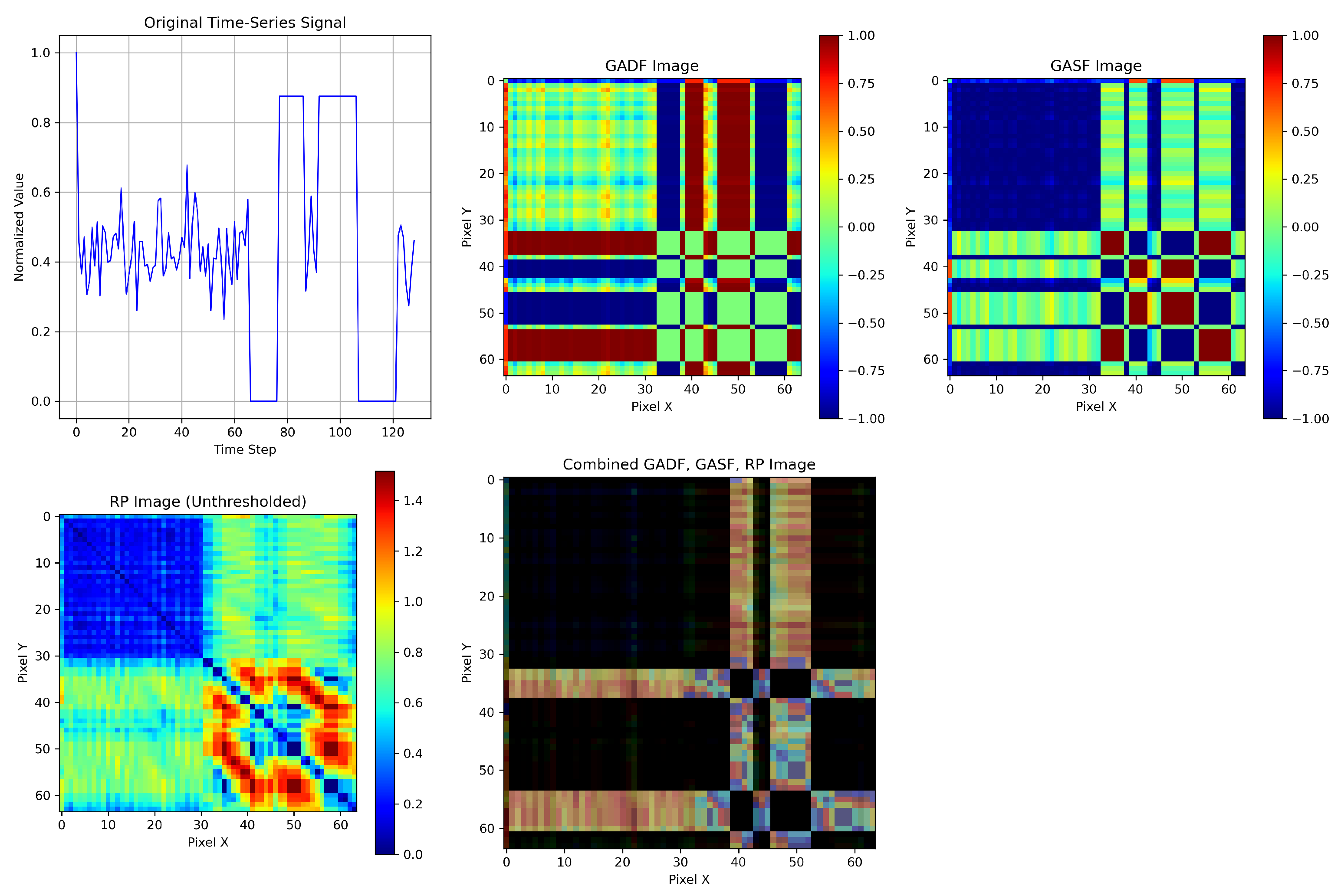
Let $X\subset {\mathbb{R}}^n$ denote the input space of univariate time series, and let $T_1,T_2,T_3:X\to {\mathbb{R}}^s\times {\mathbb{R}}^s$ represent three distinct nonlinear transformations corresponding to the Gramian Angular Summation Field (GASF), Gramian Angular Difference Field (GADF), and Recurrence Plot (RP), respectively. These transformations produce images of identical dimensions $s\times s$ via bilinear interpolation.

We define the fused image tensor as follows:

$$Z=\mathrm{concat}(T_1\left(x\right),T_2\left(x\right),T_3\left(x\right)),Z\in {\mathbb{R}}^s\times {\mathbb{R}}^s\times {\mathbb{R}}^3,$$

(10)

where concat denotes the channel-wise concatenation of the three transformed images. This operation merges multiple single-channel image representations—specifically, the RP, GASF, and GADF—into a unified three-channel tensor, analogous to an RGB image. Figure 1 illustrates the structure of the fusion strategy.

The use of concatenation along the channel dimension is a standard technique in convolutional neural networks to combine heterogeneous features into a single tensor for joint processing. A well-known example of this approach is the Inception module in GoogLeNet [24], where outputs from different convolutional filters (e.g., 1 × 1, 3 × 3, 5 × 5) are concatenated depth-wise to form a rich, multi-scale representation. In our case, channel-wise concatenation serves a similar purpose—preserving complementary information across different time-series transformations while enabling end-to-end learning via shared convolutional filters.

2.4.1. Information-Theoretic Motivation

Let $Y\in \mathcal{C}$ be the target class label. If each transform $T_i$ encodes a distinct subset of discriminative features, then the mutual information between the fused representation Z and the label Y satisfies the following:

$$I(Y;Z)\ge max\{I(Y;T_1\left(x\right)),I(Y;T_2\left(x\right)),I(Y;T_3\left(x\right))\}.$$

(11)

Under conditional independence assumptions, the joint mutual information may be approximately additive:

$$I(Y;Z)\approx I(Y;T_1\left(x\right))+I(Y;T_2\left(x\right))+I(Y;T_3\left(x\right))-\delta ,$$

(12)

where $\delta$ accounts for redundant information across transforms [25].

2.4.2. Class Separability View

Assume the conditional distributions $P(Z\mid Y=k)$ are more separable in the fused space ${\mathbb{R}}^s\times {\mathbb{R}}^s\times {\mathbb{R}}^3$ than in any single transformed space. Then, by reducing class overlap, the Bayes classification error $R^{*}$ is minimized:

$$R^{*}=\int \underset{k}{min}P(Y=k\mid Z)dZ.$$

(13)

Hence, fusion improves discriminability, especially in deep neural networks trained on Z [26].

2.4.3. Empirical Alignment

Our empirical results in

Table 2. Macro F1 score for multivariate time-series classification methods.

Method	HAR	ROE
GADF + CNN + MHA	90.51	97.53
GASF + CNN + MHA	89.21	97.45
RP + CNN + MHA	86.00	97.84
InceptionTime	85.59	98.22
MLP	81.38	89.27
Conv_1D	85.90	92.92
LSTM	81.53	86.31
GAF + ResNet	87.85	94.55
GAF + GoogLeNet	87.78	81.25
GAF + Fusion-Mdk-ResNet	89.63	96.36
Fusion + CNN + MHA	91.55	98.95

and

Table 3. Accuracy and macro F1 score for univariate time-series classification methods.

Method	FaceAll	50Words	Fish	OSULeaf	TwoPatterns	Wafer	SwedishLeaf
Accuracy
1-NN DTW	81.00	69.00	29.00	60.00	1.00	98.00	80.00
Shapelet	60.00	56.00	81.00	65.00	89.00	99.60	73.00
BoP	79.00	54.00	92.60	77.00	89.00	99.70	81.00
GAF + MTF	77.00	70.00	89.00	65.00	88.00	1.00	94.00
GADF + CNN	73.43	70.33	81.71	63.22	99.50	99.80	88.80
GASF + CNN	73.43	69.01	82.86	60.33	1.00	1.00	86.24
RP + CNN	62.31	66.81	85.71	56.61	51.15	99.59	81.80
InceptionTime	81.48	78.02	91.43	67.77	1.00	1.00	91.68
Fusion + CNN	76.51	74.07	86.86	61.16	1.00	1.00	90.70
Fusion + ResNet	80.18	76.70	89.14	78.10	1.00	1.00	92.96
Fusion + DenseNet121	94.08	81.76	96.00	85.95	1.00	1.00	94.40
Macro F1 Score
GADF + CNN	74.44	52.99	81.22	63.09	99.50	99.43	88.75
GASF + CNN	74.79	53.75	82.91	58.82	1.00	1.00	86.18
RP + CNN	64.13	46.97	85.63	53.69	50.81	98.96	81.00
InceptionTime	85.06	66.04	89.97	68.12	1.00	1.00	91.18
Fusion + CNN	77.07	59.16	86.89	60.56	1.00	1.00	90.61
Fusion + ResNet	84.13	63.77	89.08	75.89	1.00	1.00	93.00
Fusion + DenseNet121	93.17	68.10	96.05	84.11	1.00	1.00	94.44

confirm this theoretical motivation: fusion consistently improves classification performance across univariate and multivariate datasets. The improvement arises not from architectural complexity but from richer feature representation enabled by complementary views [27].

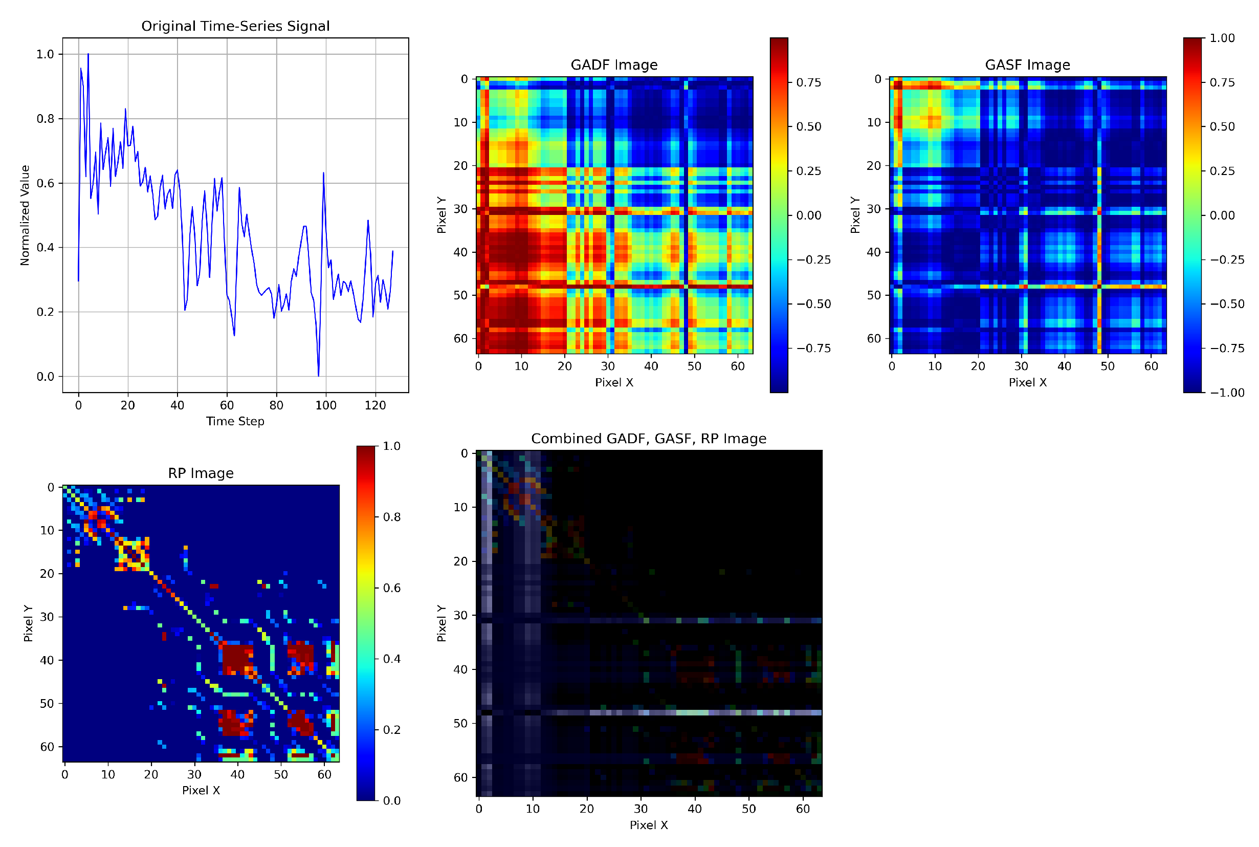
2.4.4. Special Case: Multivariate Fusion with 27 Channels

For multivariate time series, let the input be a sequence $X=[x^{\left(1\right)},x^{\left(2\right)},\dots ,x^{\left(d\right)}]\in {\mathbb{R}}^n\times {\mathbb{R}}^d$, where d is the number of sensor channels ($d=9$ for HAR). For each channel $x^{\left(k\right)}$, we apply three transformations: $T_1^{\left(k\right)}$ (GASF), $T_2^{\left(k\right)}$ (GADF), and $T_3^{\left(k\right)}$ (RP), producing the following:

$$T_i^{\left(k\right)}:{\mathbb{R}}^n\to {\mathbb{R}}^s\times {\mathbb{R}}^s,i=1,2,3;k=1,2,\dots ,d.$$

These are stacked along the channel axis to yield the fused tensor:

$$Z=\mathrm{concat}\left(T_1^{\left(1\right)},T_2^{\left(1\right)},T_3^{\left(1\right)},\dots ,T_1^{\left(d\right)},T_2^{\left(d\right)},T_3^{\left(d\right)}\right)\in {\mathbb{R}}^s\times {\mathbb{R}}^s\times {\mathbb{R}}^{3d}.$$

(14)

This design preserves both intra-channel temporal patterns and inter-channel variability. Theoretically, if each sensor channel captures unique dynamic phenomena, and each transformation extracts orthogonal features from that channel, then the fused space Z spans a richer feature manifold. An illustration of the resulting fused representations from the HAR dataset is provided in Figure 2.

Assuming partial independence among transforms and channels, the joint mutual information satisfies the following:

$$I(Y;Z)\approx \sum _{k=1}^d\sum _{i=1}^{3}I(Y;T_i^{\left(k\right)}\left(x\right))-\delta ,$$

(15)

where $\delta$ captures redundancy across transformations and channels.

This high-dimensional composite representation improves the likelihood of learning discriminative decision boundaries with deep networks, especially in complex sensor-rich environments like HAR [25,27].

2.5. Learning Architectures

2.5.1. Convolutional Neural Networks

Convolutional neural networks (CNNs) are a class of deep learning models specifically designed for image processing tasks [28]. They have proven highly effective in applications such as classification, object detection, and segmentation, due to their ability to autonomously learn hierarchical spatial features from raw data.

A typical CNN architecture consists of multiple types of layers:

• Convolutional Layers: Apply learnable filters to the input to extract local features such as edges and textures.
• Activation Functions: Introduce non-linearity, commonly using the Rectified Linear Unit (ReLU).
• Pooling Layers: Downsample feature maps using operations such as max pooling or average pooling, reducing computational complexity.
• Normalization Layers: Batch normalization is used to stabilize and accelerate the training process.
• Fully Connected Layers: Perform high-level reasoning and output final predictions.
• Dropout Layers: Randomly deactivate neurons during training to prevent overfitting.

CNNs provide two primary advantages: (i) automatic feature extraction without manual engineering and (ii) spatial invariance, as features remain stable under translations and deformations of the input.

A typical CNN architecture is illustrated in Figure 3.

2.5.2. DenseNet-121 Architecture

DenseNet (Densely Connected Convolutional Network) [29] introduces a connectivity pattern where each layer receives inputs from all preceding layers. This dense connectivity improves feature reuse, mitigates the vanishing gradient problem, and results in more parameter-efficient networks.

DenseNet-121 is a compact variant containing 121 layers, including the following:

• Dense Blocks: Each block consists of multiple convolutional layers with direct connections.
• Transition Layers: 1 × 1 convolution followed by pooling to compress features between dense blocks.

This architecture facilitates efficient feature propagation and improves model generalization, making it particularly suitable for classification tasks on time-series images. In this study, DenseNet-121 is employed for univariate time-series classification after GAF-RP image fusion.

The structure of DenseNet-121 is illustrated in Figure 4.

2.5.3. Multi-Head Attention Mechanism

Multi-Head Attention (MHA) [30] is a key component of Transformer-based architectures. It enables models to weigh the relevance of different input elements dynamically, thereby capturing contextual dependencies across the sequence. The core idea is that the model can “attend” to various parts of the input differently for each position.

Scaled Dot-Product Attention

Given three input matrices: queries $Q\in {\mathbb{R}}^n\times {\mathbb{R}}^{d_k}$, keys $K\in {\mathbb{R}}^n\times {\mathbb{R}}^{d_k}$, and values $V\in {\mathbb{R}}^n\times {\mathbb{R}}^{d_v}$, the attention mechanism computes the following:

$$\mathrm{Attention}(Q,K,V)=\mathrm{softmax}\left({\displaystyle \frac{Q{K}^T}{\sqrt{d_k}}}\right)V.$$

(16)

Here,

• $Q{K}^T$ measures the similarity between queries and keys via dot product.
• $\sqrt{d_k}$ scales the similarity scores to maintain numerical stability.
• Softmax transforms these scores into a probability distribution, allowing the model to focus selectively on more relevant inputs. Formally, for a vector $\mathbf{x}\in {\mathbb{R}}^n$, softmax is defined as follows:

  $$\mathrm{softmax}\left(x_i\right)={\displaystyle \frac{e^{x_i}}{{\sum }_{j=1}^n{e}^{x_j}}},\mathrm{for}i=1,\dots ,n.$$

  (17)
• The weighted combination of values V yields a context-aware representation of the input.

This operation enables the model to dynamically focus on different parts of the input sequence by computing the relevance of each key to a given query. The softmax function ensures the attention scores form a probability distribution, and the weighted sum aggregates the most relevant information from the values. This mechanism allows the network to capture long-range dependencies and contextual interactions effectively.

Softmax, introduced in the context of probabilistic modeling, is widely used in neural networks to convert raw activations into interpretable probabilities [31].

Multi-Head Attention (MHA)

Instead of relying on a single attention mechanism, MHA projects the inputs into multiple subspaces via learned weight matrices $W_i^Q,W_i^K,W_i^V$, and computes the following:

$${\mathrm{head}}_i=\mathrm{Attention}(Q{W}_i^Q,K{W}_i^K,V{W}_i^V).$$

(18)

The outputs from all attention heads are concatenated and linearly transformed:

$$\mathrm{MultiHead}(Q,K,V)=\mathrm{concat}({\mathrm{head}}_1,\dots ,{\mathrm{head}}_h)W^O,$$

(19)

where $W^O$ is a learnable projection matrix. This mechanism allows the model to capture diverse relationships from different representation subspaces simultaneously.

For an intuitive visualization and practical overview of attention mechanisms, see [32].

In this work, we combine a CNN backbone with Multi-Head Attention to enhance multivariate time-series classification by learning both local spatial features and global dependencies across feature channels. An overview of the Multi-Head Attention mechanism and the proposed CNN + Attention architecture is shown in Figure 5.

2.6. Bayesian Optimization for Image Size Tuning

Bayesian Optimization (BO) is a model-based global optimization technique designed to optimize expensive, black-box objective functions with minimal evaluations [33,34]. In our work, BO is employed to determine the optimal image dimension $x\in \mathcal{X}\subseteq \mathbb{Z}$ that maximizes model performance (e.g., classification accuracy or macro F1-score) across different transformation pipelines.

2.6.1. Motivation for Image Size Tuning

The performance of deep learning models applied to time-series image representations (e.g., GASF, GADF, RP) is sensitive to the resolution of the input images. Fixed image sizes may underrepresent fine details or introduce unnecessary redundancy. Hence, automatic image size tuning ensures an optimal balance between information retention and model complexity, especially when transforming time series into 2D images.

2.6.2. Problem Formulation

Let $f\left(x\right):\mathcal{X}\to \mathbb{R}$ denote the objective function mapping a given image size x to the performance metric (e.g., validation accuracy). The goal is to find the following:

$$x^{*}=arg\underset{x\in \mathcal{X}}{max}f\left(x\right),$$

(20)

where $\mathcal{X}\subseteq [32,128]$ represents the discrete search space of candidate image dimensions. Evaluating $f\left(x\right)$ entails training a deep model with transformed images resized to $x\times x$, which is computationally expensive.

2.6.3. Bayesian Optimization Pipeline

BO addresses this challenge by modeling $f\left(x\right)$ as a stochastic process and selecting sample points efficiently. The pipeline consists of the following core components:

Surrogate Modeling via Gaussian Processes

A Gaussian Process (GP) [35] is used to approximate $f\left(x\right)$. It provides a posterior mean $\mu \left(x\right)$ and variance ${\sigma }^2\left(x\right)$, capturing both prediction and uncertainty:

$$f\left(x\right)\sim \mathcal{GP}(\mu \left(x\right),k(x,x^{\prime })),$$

(21)

where $k(x,x^{\prime })$ is a covariance kernel (e.g., squared exponential). In BO, we are interested in maximizing an unknown and potentially expensive-to-evaluate objective function $f\left(x\right)$, where $x\in \mathcal{X}$ is a continuous or discrete hyperparameter (e.g., image size). Instead of evaluating all possible $x\in \mathcal{X}$, BO uses prior beliefs about $f\left(x\right)$ and updates these beliefs using observed data to compute a posterior distribution. This process reflects the core Bayesian paradigm:

$$\mathrm{Posterior}\propto \mathrm{Likelihood}\times \mathrm{Prior}.$$

(22)

The posterior is used to reason about uncertainty and to make informed decisions about where to sample next.

Acquisition Function

To decide which image size to evaluate next, BO employs an acquisition function $a\left(x\right)$, such as Expected Improvement (EI) [36], which balances exploration and exploitation:

$$a\left(x\right)=\mathbb{E}\left[max(0,f\left(x\right)-f\left(x_{\mathrm{best}}\right))\right].$$

(23)

This function favors regions with high uncertainty or promising predicted performance.

Iterative Sampling

BO proceeds by

• Initializing with n randomly chosen image sizes and their evaluated performance.
• Fitting the GP model to these samples.
• Selecting the next x by maximizing $a\left(x\right)$.
• Evaluating $f\left(x\right)$ via model training and recording the result.
• Updating the GP model and repeating until convergence or a maximum budget is reached.

Final Output

The image size $x^{*}$ with the highest observed score is selected:

$$x^{*}=arg\underset{x\in \mathcal{X}}{max}f\left(x\right).$$

(24)

2.6.4. Application and Advantages in Our Framework

In our framework, Bayesian Optimization is employed independently for each dataset and transformation fusion pipeline to automatically determine the optimal image resolution that maximizes classification performance. This replaces the need for manual or exhaustive grid search and allows the model to adaptively identify the most suitable image size based on the characteristics of each dataset. The optimization is performed under a constrained evaluation budget (e.g., 10 iterations), ensuring computational efficiency.

This application of BO brings several benefits to our image-based time-series classification task. First, it significantly reduces the number of training runs required to find an effective configuration, making the process more efficient. Second, it provides adaptivity by tailoring image dimensions to the structural and temporal properties of the data. Third, and most importantly, it results in performance gains, as evidenced by our experimental results showing improved classification accuracy and macro F1-score when using BO-tuned image sizes. By leveraging probabilistic modeling and principled acquisition strategies, BO offers a data-efficient and robust approach for tuning image size—an otherwise overlooked yet impactful hyperparameter—thus enhancing the overall generalizability and effectiveness of the proposed classification pipeline.

3. Results

3.1. Reproducibility and Hyperparameter Settings

To ensure reproducibility and address transparency in our experimental setup, we detail the key preprocessing hyperparameters and implementation choices used for generating the image-based representations and training the classification models.

3.1.1. Recurrence Plot (RP) Parameters

For the univariate time series, we used the unthresholded recurrence plot to retain fine-grained recurrence structures. In this case, no threshold $\epsilon$ is required. The embedding dimension and time delay were set to $m=3$ and $\tau =4$, respectively, for all datasets. These values were selected based on empirical validation and prior literature [37], and we confirmed their generalizability by comparing them with alternative settings, where they consistently yielded better classification performance.

For the multivariate time-series datasets, we employed dataset-specific configurations of the Recurrence Plot class to tailor recurrence structure to signal characteristics and maintain consistency in sparsity levels across varying scales.

For the HAR dataset, we used an embedding dimension of $m=3$ and a time delay of $\tau =2$, combined with pointwise thresholding. Under this scheme, $\epsilon$ corresponds to the 10th percentile of all pairwise distances between embedded points, as determined by the default percentage $=10$ in pyts.image.RecurrencePlot, yielding a sparse binary recurrence plot.

For the ROE dataset, we applied a distance-based threshold by setting threshold = ‘distance’ and specifying percentage = 20, which computes the threshold $\epsilon$ as the 20th percentile of all pairwise distances in the embedded space. This method provides relative consistency in sparsity regardless of signal scale or variability. The embedding parameters were kept minimal with $m=1$ and $\tau =1$ to enhance interpretability and reduce noise.

These tailored configurations ensure that the recurrence structures encoded into the images reflect the most relevant temporal dynamics of each dataset.

3.1.2. Bayesian Optimization Setup

To optimize the image dimension used for input to the deep models, we employed Bayesian Optimization. We used a total of 30 iterations for the univariate case and 10 iterations for the multivariate case. These choices were guided by the need to balance search coverage and computational cost, particularly due to the high training time of deep models on larger images.

The search bounds were set to $[32,128]$ based on common input dimensions in related deep learning literature for time-series classification [2]. This range offers a balance between resolution and model tractability, allowing both fine and coarse representations to be evaluated. We opted for Bayesian Optimization over simple grid search or default sizes because BO explores the parameter space more efficiently and adapts to the underlying response surface, leading to empirically better results under limited evaluation budgets.

3.2. Model Architectures and Training Protocols

3.2.1. Fusion Model for Multivariate Datasets

We used a hybrid CNN and attention-based architecture to process fused image representations from RP, GASF, and GADF. The model configuration is as follows:

• Conv2D layers: 64, 128, 256 filters with kernel size $(3\times 3)$ and ReLU activation; same padding and MaxPooling2D after each block.
• Normalization: Batch normalization after each convolutional layer.
• Reshape: Spatial features reshaped to a temporal sequence of shape $(16\times 16,256)$.
• Attention: Multi-Head Attention with four heads and a key dimension of 256, followed by layer normalization.
• Dense layers: Two fully connected layers of sizes 512 and 256 with ReLU, Dropout(0.5), and softmax output.
• Optimization: Adam optimizer with learning rate = 0.0005; loss = sparse categorical crossentropy.

3.2.2. Fusion Model for Univariate Datasets

For univariate datasets, we used a DenseNet121-based architecture to process the fused images. The architecture is configured as follows:

• Base: DenseNet121 (weights = ‘imagenet’, include_top = False) with three-channel RGB input.
• Top layers: GlobalAveragePooling2D, Dense(1024, ReLU), BatchNormalization, Dropout(0.5), Dense(output classes, softmax).
• Optimization: Adam optimizer with learning rate = 0.0001; loss = categorical crossentropy.

3.2.3. CNN for Individual Transformations

For the individual univariate transformations (RP, GASF, and GADF), we used a lightweight customized CNN consisting of two convolutional layers with 32 and 64 filters, kernel sizes of $(5\times 5)$ and $(3\times 3)$, respectively, each followed by max pooling with a pool size of $(2\times 2)$. A batch normalization layer and dropout layer with a rate of 0.3 were included to improve generalization. The flattened output was passed through a dense layer with 128 units and a dropout rate of 0.5 before the final softmax output layer. The model was compiled with the Adam optimizer (learning rate = 0.0001), using categorical crossentropy as the loss function and accuracy as the evaluation metric. This model was specifically designed to handle single-channel grayscale images efficiently.

To ensure that performance differences reflect the discriminative power of the image transformations rather than model complexity, we used a modified version of the same CNN architecture for the fused RGB image combining GADF, GASF, and RP. The architecture was adapted to process three-channel input by adjusting only the input shape, preserving the rest of the architecture. This strategy ensures a fair comparison and isolates the contribution of the proposed image fusion technique.

For the individual multivariate transformations, we used the same CNN architecture employed in the fusion model, which includes three convolutional layers, Multi-Head Attention (MHA), and dense layers. This ensured consistency in depth and capacity across the individual and fused representations for the multivariate case.

3.2.4. Fusion + ResNet50 for Univariate Time Series

To further assess the strength of the proposed fused image representations, we applied the ResNet50 architecture to the univariate datasets. ResNet50 is a deep convolutional neural network with residual connections that is widely recognized for its robustness in image classification tasks [38,39]. In our framework, it was exclusively applied to the fused images—comprising GADF, GASF, and RP channels—thereby serving as a benchmark to test whether performance gains originated from the fusion strategy rather than from architectural complexity.The model was fine-tuned using a learning rate of 0.0001 and trained with categorical crossentropy loss. We did not apply ResNet50 to the multivariate datasets, as existing comparative baselines already incorporated ResNet variants (e.g., GAF + ResNet, GAF + Fusion-Mdk-ResNet). This selective usage isolates the contribution of the fusion strategy in the univariate setting and ensures a fair architectural comparison.

3.2.5. InceptionTime Baseline

As an additional baseline, we trained the InceptionTimeClassifier from the sktime library using default parameters [8]. For ROE, we first applied a sliding window of size 30 (no overlap), whereas the HAR dataset already consists of pre-windowed sequences of 128 time steps.

3.2.6. Training Settings

Batch size was selected from the set $\{5,20,32,64\}$ depending on the dataset size and GPU memory availability. The number of training epochs was chosen from $\{20,50,100,200\}$ based on preliminary validation performance for each model and dataset. Early stopping was not applied; instead, training was conducted for the full number of selected epochs in each case to ensure consistency and fairness across experiments.

3.3. Evaluation Strategy and Metrics

To ensure a fair and reproducible evaluation, all models—including the proposed fusion framework, individual transformations (RP, GASF, GADF), and baseline models such as InceptionTime—were trained using the same data splits and without any data augmentation. Each image-based method employed consistent preprocessing pipelines and CNN architectures tailored to the univariate or multivariate nature of the dataset.

Since some of the univariate datasets exhibit class imbalance, we report both classification accuracy and macro-averaged F1 score to reflect overall and per-class performance. For multivariate datasets, we report only the macro F1 score due to their more significant class imbalance. To streamline the results presentation, we do not include full precision and recall metrics across all datasets. Instead, confusion matrices for the HAR and ROE datasets are provided to visually highlight class-wise prediction strengths and weaknesses of the proposed fusion model.

Accuracy measures the proportion of correctly classified instances out of the total number of samples. It is defined as follows:

$$\mathrm{Accuracy}={\displaystyle \frac{{\sum }_{i=1}^N\mathbb{I}({\widehat{y}}_i=y_i)}{N}},$$

(25)

where N is the total number of test instances, ${\widehat{y}}_i$ is the predicted label, $y_i$ is the true label, and $\mathbb{I}(·)$ is the indicator function that returns 1 when its argument is true, and 0 otherwise.

The macro-averaged F1 score computes the F1 score independently for each class and then takes the unweighted mean. It is defined as follows:

$$\mathrm{Macro}\text{-}\mathrm{F}1={\displaystyle \frac{1}{C}}\sum _{c=1}^C{\mathrm{F}1}_c={\displaystyle \frac{1}{C}}\sum _{c=1}^C{\displaystyle \frac{2·{\mathrm{Precision}}_c·{\mathrm{Recall}}_c}{{\mathrm{Precision}}_c+{\mathrm{Recall}}_c}},$$

(26)

where C is the number of classes, and ${\mathrm{Precision}}_c$ and ${\mathrm{Recall}}_c$ are defined for each class c as follows:

$${\mathrm{Precision}}_c={\displaystyle \frac{T{P}_c}{T{P}_c+F{P}_c}},{\mathrm{Recall}}_c={\displaystyle \frac{T{P}_c}{T{P}_c+F{N}_c}},$$

(27)

with $T{P}_c$, $F{P}_c$, and $F{N}_c$ denoting the true positives, false positives, and false negatives for class c, respectively.

3.4. Ablation Study and Comparison with Existing Methods

Table 2 and Table 3 present the results of our ablation study, which compares the performance of individual image transformations—Recurrence Plot (RP), Gramian Angular Summation Field (GASF), and Gramian Angular Difference Field (GADF)—against the proposed fusion strategy. All models were trained under identical conditions, using the same preprocessing, architecture, and training protocol, thereby ensuring a fair evaluation.

The fusion approach, which combines both recurrence-based and angular-based representations, consistently outperforms the individual transformations on both univariate and multivariate datasets in terms of accuracy and macro F1 score. This highlights the complementarity between local recurrence structures and global angular patterns.

Figure 6 displays confusion matrices for the multivariate HAR and ROE datasets, further validating the improved class-level discrimination of the fusion model.

To provide broader context, we also benchmark our method against state-of-the-art models from the literature. As shown in Table 2 and Table 3, these include traditional methods such as 1-NN DTW, Shapelet Transform, and Bag-of-Patterns (BoP), as well as deep learning models like ResNet, and other GAF-based architectures.

Note that for baselines sourced from prior works, we retained the reported results without retraining. Specifically, 1-NN DTW, Shapelet, BoP, and GAF + MTF were adopted directly from [37]. For HAR, the results of MLP, Conv_1D, LSTM, and ResNet variants were reproduced from [40]; however, since [40] did not evaluate on ROE, we implemented these methods for ROE using consistent experimental settings.

4. Discussion

4.1. Performance Insights

The experimental results clearly demonstrate the effectiveness of the proposed fusion-based model across a diverse set of univariate and multivariate time-series datasets. For univariate classification, the Fusion + DenseNet121 configuration achieved the highest macro F1 scores across all seven benchmark datasets, substantially outperforming both traditional approaches (e.g., 1-NN DTW, Shapelet, BoP) and single-transformation CNN models. Similarly, for multivariate data, the Fusion + CNN + MHA model delivered superior performance on HAR and ROE datasets, reaching macro F1 scores of 91.55 and 98.95, respectively.

These improvements are attributed to the complementary nature of the recurrence and angular features captured by RP, GASF, and GADF. Recurrence plots preserve local structural patterns, while GAF-based transformations capture global temporal dependencies. The integration of these modalities enriches the representational capacity of the model, enabling it to distinguish between fine-grained temporal patterns that are often indistinguishable using a single transformation.

4.2. Comparison with Prior Work

Compared to state-of-the-art methods from the literature, the proposed framework establishes new benchmarks on multiple datasets. Traditional time-series classifiers such as 1-NN DTW and Shapelet-based methods often fall short due to their reliance on hand-crafted distance metrics or rigid pattern matching. Even modern deep learning models, such as InceptionTime or single-transform CNNs, exhibit limitations when applied in isolation. Our results show that the fusion model not only surpasses these baselines in accuracy and F1 score but also generalizes well across domains.

Notably, for models such as 1-NN DTW, Shapelet, BoP, and GAF + MTF, we adopted results directly from prior studies [37]. Similarly, HAR results for MLP, Conv_1D, LSTM, and ResNet-based methods were sourced from [40], while we implemented these models for the ROE dataset under consistent conditions. All other results were generated using our unified experimental setup to maintain consistency across methods.

4.3. Confusion Matrix Interpretation

The confusion matrices presented in Figure 6 highlight the class-level performance of the fusion model. On the HAR dataset, the model demonstrates strong discrimination among similar activities, though minor confusion is observed between “Sitting” and “Standing”—a common challenge due to overlapping postural signals. For the ROE dataset, the model excels across all occupancy levels, including rare classes, indicating robustness to class imbalance.

4.4. Practical Relevance and Generalization

The observed performance gains across both balanced and imbalanced datasets confirm the generalizability of the proposed approach. The fusion strategy is especially effective in real-world applications such as human activity recognition and smart building analytics, where sensor signals are noisy, heterogeneous, and multi-channel. Furthermore, the use of Bayesian Optimization for selecting transformation parameters enhances both accuracy and computational efficiency, eliminating the need for manual tuning.

4.5. Limitations and Future Work

Despite its strong performance, the fusion model introduces increased computational costs due to the 27-channel input derived from stacking GASF, GADF, and RP transformations across multiple sensors. This can lead to high memory usage and longer training times. Future research will explore dimensionality reduction strategies, such as learning attention-based weights for selecting the most informative transformations or sensor channels.

5. Conclusions

This study introduced GAF-RP-CNN-BO, a novel framework for time-series classification that fuses Gramian Angular Fields (GASF and GADF) with recurrence plots (RPs) to generate rich image representations of temporal data. Bayesian Optimization was employed to automatically determine optimal image dimensions, eliminating manual tuning and improving classification performance.

Extensive experiments on seven univariate and two multivariate benchmark datasets demonstrated that the proposed method consistently outperformed traditional approaches such as 1-NN DTW, Shapelet Transform, and single-modality CNNs. The fusion model, coupled with DenseNet121 for univariate tasks and CNN with Multi-Head Attention for multivariate tasks, achieved the highest accuracy and macro F1 scores across datasets.

Future research will explore the development of a meta-learning framework capable of automatically selecting the most suitable transformation method based on dataset-specific characteristics. This would further reduce manual intervention in the preprocessing pipeline and enhance adaptability across diverse domains. In addition, future efforts will focus on extending the applicability of the proposed method to underexplored areas such as financial forecasting, clinical diagnostics, and environmental monitoring, where accurate time-series classification remains a critical and impactful challenge.