Modeling and Exploration of Localized Wave Phenomena in Optical Fibers Using the Generalized Kundu–Eckhaus Equation for Femtosecond Pulse Transmission

Abstract

This manuscript aims to explore localized waves for the nonlinear partial differential equation referred to as the $(1+1)$-dimensional generalized Kundu–Eckhaus equation with an additional dispersion term that describes the propagation of the ultra-short femtosecond pulses in an optical fiber. This research delves deep into the characteristics, behaviors, and localized waves of the $(1+1)$-dimensional generalized Kundu–Eckhaus equation. We utilize the multivariate generalized exponential rational integral function method (MGERIFM) to derive localized waves, examining their properties, including propagation behaviors and interactions. Motivated by the generalized exponential rational integral function method, it proves to be a powerful tool for finding solutions involving the exponential, trigonometric, and hyperbolic functions. The solutions we found using the MGERIF method have important applications in different scientific domains, including nonlinear optics, plasma physics, fluid dynamics, mathematical physics, and condensed matter physics. We apply the three-dimensional (3D) and contour plots to illuminate the physical significance of the derived solution, exploring the various parameter choices. The proposed approaches are significant and applicable to various nonlinear evolutionary equations used to model nonlinear physical systems in the field of nonlinear sciences.

1. Introduction

The study of nonlinear partial differential equations (NPDEs) holds great importance in various branches of science and engineering, as they describe a wide range of physical phenomena. Among the many intriguing equations in this field, the $(1+1)$-dimensional generalized Kundu–Eckhaus equation (GKEE) stands out as a fundamental and challenging equation, known for its rich dynamics and remarkable mathematical proper attention due to its ability to describe diverse physical phenomena, including wave propagation in nonlinear media, plasma physics, fiber optics, and Bose–Einstein condensates. The equation exhibits a nonlinear dispersion effect, where the wave velocity depends on the wave amplitude, leading to intriguing and complex dynamics.

Various analytical techniques can be employed in the resolution of Nonlinear Partial Differential Equations (NLPDEs) and the generation of traveling wave solutions such as the extended ${\displaystyle \frac{G^{\prime }}{G}}$ expansion method [1,2], and the extended trial equation method [3,4,5]. Others can be found in the middle of these. The Riccati-sub-ODE Bernoulli’s method [6], the first integral method [7,8], the truncated expansion method [9], the sub-equation method [10,11], the modified simple equation method [12,13], the extended Jacobi’s elliptic function method [14,15,16], the Lie symmetry analysis [17,18], the new extended direct algebraic method [19,20], Hirota bilinear method [21], KP hierarchy reduction [22], Riemann–Hilbert approach [23], Hirota bilinear method [24,25,26,27], stability analysis [28,29], chaos and bifurcation behavior [30,31,32,33,34,35,36], sine–cosine method [37,38], and many more methods [39].

Kundu and Eckhaus are the authors of the first publication of the GKEE, a variation of the well-known nonlinear Schrödinger equation. Since then, it has drawn a lot of interest because of its capacity to explain a wide range of physical phenomena, including wave propagation in nonlinear media, plasma physics, fiber optics, and Bose-Einstein condensates. The equation displays a nonlinear dispersion effect, which results in fascinating and complex dynamics where the wave velocity depends on the wave amplitude.

The GKEE is a complex-valued NPDE that combines nonlinear and dispersive terms mathematically. It symbolizes the interaction between nonlinearity and dispersion, frequently resulting in the development and spread of solitons, localized wave packets with stable shapes. Despite the numerous uses and importance of GKEE, little is known about its analytical capabilities and precise solutions. Therefore, it is crucial to gain a deeper understanding of the behavior of the equation and its soliton solutions.

The multivariate generalized exponential rational integral function method (MGERIFM) is a newly developed technique to solve the NLPDEs and find the exact solutions. M Niwas et al. [40] used this method and solved the (2+1)-dimensional Hirota bilinear equation to find the exact solutions. Usman et al. [41] applied this method to the nonlinear fractional longitudinal wave equation. Jan et al. [42] studied the multicomponent nonlinear Schrödinger equation by applying the MGERIFM. Muhammad et al. [43] solved the Gross–Pitaevskii model in Bose–Einstein condensates and communication systems by MGERIFM.

A complex-valued wave amplitude $\mathfrak{B}=\mathfrak{B}(x,t)$ evolves in space and time according to the nonlinear partial differential equation known as the GKEE with an extra-dispersion. The equation is given by [44]

$$i{\mathfrak{B}}_t+A{\mathfrak{B}}_{xx}+i{d}_1{\mathfrak{B}}_{xxx}+d_2{\mathfrak{B}}_{xxxx}+{G\left|\mathfrak{B}\right|}^2\mathfrak{B}+B_2{\left|\mathfrak{B}\right|}^4\mathfrak{B}-{2iB\left(\right|\mathfrak{B}|}^2{)}_x\mathfrak{B}=0,$$

(1)

where i is the fictitious unit, $\mathfrak{B}=\mathfrak{B}(x,t)$ is the complex smooth envelop function, and $A,d_1,d_2,G,B$ and $B_2$ are constants. In this equation, A is the coefficient of weak dispersion, and x and t are the spatial and temporal variables, respectively. Real constant B is followed by the cubic and quintic nonlinearity coefficients (G and $B^2$, respectively), which are the third- and fourth-order of extra dispersion coefficient $(d_1,d_2)$ and the Riemann effect in the last term.It should be noted that the symbol G represents either self-focusing or self-defocusing polarized pulses, depending on its sign, whether it is + or −. The first term on the left represents the wave’s temporal history, while the dispersion and higher-order dispersion are represented by the second and third terms, respectively. The fourth term, the nonlinear term, represents the self-interaction of the wave due to the medium’s nonlinear properties. The fifth and sixth terms are higher-order nonlinear effects that explain why the medium is nonlinear at larger powers of the wave amplitude. The extra-dispersion term, which comes last, accounts for the impact of the wave envelope on the dispersion. The remainder of the paper is organized as follows:

Section 2 provides a detailed formulation of the Generalized Kundu–Eckhaus equation and explains the process of transforming nonlinear partial differential equations (PDEs) into nonlinear ordinary differential equations (ODEs). Section 3 describes the innovative steps of the multivariate generalized exponential rational integral function approach and its application. This includes various forms of representation, such as sine, cosine, exponential, hyperbolic cosine, and hyperbolic sine descriptions, along with graphical illustrations using appropriate parametric values. Section 4 explores the implications of the findings, highlights potential applications, and suggests future research directions, supported by graphical representations. Section 5 provides a concise summary of the graphical visualizations. Finally, Section 6 presents the overall conclusion.

2. Mathematical Analysis and Modeling

General nonlinear PDEs have the form

$$\Theta (\mathfrak{B},{\mathfrak{B}}_x,{\mathfrak{B}}_{xt},{\mathfrak{B}}_{xxx}...)=0,$$

(2)

where the unknown function $\mathfrak{B}=\Phi (x,t)$. By applying the specified transformations, it becomes possible to transform the given nonlinear partial differential Equation (1) into an ordinary differential equation (ODE) by insertion of the transformation:

$$\mathfrak{B}(x,t)=\Phi \left(\xi \right)e^{\iota (\kappa x-\Omega t+c)},\xi =\theta x+\rho t,$$

(3)

where $\kappa$ and $\Omega$ are real fixed parameters that show the frequency shift and the wave number. In addition, c stands for the phase constant, $\theta$ is a real constant, and $\rho$ stands for the speed of the soliton. Putting Equation (3) in place of Equation (1), We get the ODE of the form

$$\Theta (\Phi ,{\Phi }^{\prime },{\Phi }^{″},{\Phi }^{‴},...)=0.$$

(4)

Substituting Equation (3) in Equation (1), we change Equation (1), then we obtain real and imaginary parts as

$$d_2{\theta }^4{\displaystyle \frac{d\Phi }{d{\xi }^4}}+{\theta }^2(A-6d_2{k}^2-3d_{1}k){\displaystyle \frac{d^2\Phi }{d{\xi }^2}}+(-A{k}^2+d_2{k}^4+d_1{k}^3+\Omega )\Phi +G{\Phi }^3+B_2{\Phi }^5=0,$$

(5)

and,

$$\left(2A\theta \kappa -4d_2\theta {\kappa }^3-3d_1\theta {\kappa }^2+\rho \right){\displaystyle \frac{d\Phi }{d\xi }}-4B\theta {\Phi }^2{\displaystyle \frac{d\Phi }{d\xi }}+{\theta }^3\left(4d_2\kappa +d_1\right){\displaystyle \frac{d^3\Phi }{d{\xi }^3}}=0.$$

(6)

For simplicity, we assume that

$$\rho =4d_2\theta {\kappa }^3+3d_1\theta {\kappa }^2-2A\theta \kappa$$

(7)

and Equation (6) can be transformed as follows:

$${\theta }^3\left(4d_2\kappa +d_1\right){\displaystyle \frac{d^3\Phi }{d{\xi }^3}}-4B\theta {\Phi }^2{\displaystyle \frac{d\Phi }{d\xi }}=0.$$

(8)

By applying the integration to Equation (8) and letting the integration be zero, we obtain

$${\displaystyle \frac{d^2\Phi }{d{\xi }^2}}={\displaystyle \frac{4B{\Phi }^3}{3{\theta }^2\left(4d_2\kappa +d_1\right)}}.$$

(9)

Using Equation (9), Equation (5) can be represented as follows:

$$a{\Phi }^5+b{\Phi }^3+c\Phi +g{\displaystyle \frac{d^4\Phi }{d{\xi }^4}}=0,$$

(10)

where, $a=12B_2{d}_2\kappa +3B_2{d}_1$, $b=4AB-24B{d}_2{\kappa }^2-12B{d}_1\kappa +12d_2\kappa G+3d_{1}G$, $c=-12A{d}_2{\kappa }^3-3A{d}_1{\kappa }^2+12d_2^2{\kappa }^5+15d_1{d}_2{\kappa }^4+3d_1^2{\kappa }^3+12d_2\kappa \Omega +3d_1\Omega$, $g=12d_2^2{\theta }^4\kappa +3d_1{d}_2{\theta }^4$.

3. Multivariate Generalized Exponential Rational Integral Function Approach

We proudly unveil the multivariate generalized exponential rational integral function approach (MGERIF), a groundbreaking and highly efficient methodology. This revolutionary MGERIF strategy, meticulously explored in [40], is distinguished by its unparalleled capacity to generate innovative and trans formative solutions to NLPDEs. Built on the foundation of the generalized exponential rational integral function approach [45,46], this method excels in addressing complex mathematical challenges. Its significance lies in its ability to handle NLPDEs efficiently, providing a reliable method for addressing complex problems. The basic steps of MGERIF are as follows:

Step 01: 

MGERIF provides the solution of Equation (1) as follows:

$$\Phi \left(\xi \right)=\alpha +\sum _{j=1}^N{\beta }_j{\left(\underset{j}{\underbrace{\int \dots \int }}\mathfrak{P}\left(\xi \right)d\xi d\xi \dots d\xi \right)}^j+\sum _{j=1}^N{\delta }_j{\left(\underset{j}{\underbrace{\int \dots \int }}\mathfrak{P}\left(\xi \right)d\xi d\xi \dots d\xi \right)}^{-j}.$$

(11)

where $\alpha$, ${\beta }_j$, ${\delta }_j$ (for j = 1, 2,..., N) are constants, and the function $\mathfrak{P}\left(\xi \right)$ verifies the relation

$$\mathfrak{P}\left(\xi \right)={\displaystyle \frac{p_1{e}^{q_1\xi }+p_2{e}^{q_2\xi }}{p_3{e}^{q_3\xi }+p_4{e}^{q_4\xi }}}.$$

(12)

where $p_j,q_j$ (for j = 1, 2, 3, 4) are the parameters. By setting their values, we can write Equation (12) in some familiar representations.

• When $[p_1,p_2,p_3,p_3]=[1,-1,i,i]$ and $[q_1,q_2,q_3,q_4]=[i,-i,0,0]$ then

  $$\mathfrak{P}\left(\xi \right)=sin\left(\xi \right).$$

  (13)
• When $[p_1,p_2,p_3,p_3]=[1,1,1,1]$ and $[q_1,q_2,q_3,q_4]=[i,-i,0,0]$ then

  $$\mathfrak{P}\left(\xi \right)=cos\left(\xi \right).$$

  (14)
• When $[p_1,p_2,p_3,p_3]=[2,2,2,2]$ and $[q_1,q_2,q_3,q_4]=[2/5,2/5,0,0]$ then

  $$\mathfrak{P}\left(\xi \right)=e^{{\displaystyle \frac{2\xi }{5}}}.$$

  (15)
• When $[p_1,p_2,p_3,p_3]=[i,i,i,i]$ and $[q_1,q_2,q_3,q_4]=[1,-1,0,0]$ then

  $$\mathfrak{P}\left(\xi \right)=cosh\left(\xi \right).$$

  (16)
• When $[p_1,p_2,p_3,p_3]=[2i,-2i,4i,4i]$ and $[q_1,q_2,q_3,q_4]=[1/2,-1/2,0,0]$ then

  $$\mathfrak{P}\left(\xi \right)={\displaystyle \frac{1}{2}}sinh\left({\displaystyle \frac{\xi }{2}}\right).$$

  (17)

Step 02: 

Using the homogeneous balance principle, we may get the positive integer N by balancing the highest-order derivative and nonlinear variables in Equation (3).

Step 03: 

After inserting Equations (11) and (12) in Equation (3) as a result of this substitution, we get a polynomial of $e^{nj\xi }$ with $1\le j\le 4$. Equivalently, setting all terms with the same power equal to zero. Then by solving this set of nonlinear algebraic systems with the help of Equation (12), the solutions of Equation (1) may be determined.

Step 04: 

Using mathematical reductions through software such as Mathematica, we may determine the precise values of the variables $\alpha ,{\beta }_j,$ and ${\delta }_j$$(1\le j\le N)$. Upon determining these values, we may replace them with Equations (11) and (12), enabling us to derive precise soliton solutions for Equation (1).

3.1. Solutions by MGERIF Method

To find the exact solution of Equation (3), firstly obtain a value of the positive integer $N=2$ and by inserting N in Equation (11):

$$\Phi \left(\xi \right)=\alpha +{\beta }_1\left(\int \mathfrak{P}\left(\xi \right)d\xi \right)+{\displaystyle \frac{{\delta }_1}{\int \mathfrak{P}\left(\xi \right)d\xi }}.$$

(18)

We get a series of results for Equation (3) by substituting the resulting solution into Equation (3), along with Equation (2), and using the MGERIF approach using computing tools like Mathematica.

3.2. The Familiar Sin Description

By setting the values of parameters to $[p_1,p_2,p_3,p_3]=[1,-1,i,i]$ and $[q_1,q_2,q_3,q_4]=[i,-i,0,0]$, Equation (12) is converted into standard sin representation

$$\mathfrak{P}\left(\xi \right)=sin\left(\xi \right).$$

(19)

Putting Equation (19) in Equation (11), we conclude with the expression as

$$\Phi \left(\xi \right)=\alpha -{\beta }_{1}cos\left(\xi \right)-{\delta }_{1}sec\left(\xi \right).$$

(20)

• Case 1.1:
  $\alpha ,{\beta }_1,{\delta }_1$ are not equal to zero, $d_1={\displaystyle \frac{2A}{3K}}$, and $d_2=-{\displaystyle \frac{6}{6k^2}}.$ Incorporating the values of these parameters in Equation (20), the result of the corresponding Equation (3) is obtained.

  $$\Phi \left(\xi \right)=\alpha -{\beta }_{1}cos\left(\xi \right)-{\delta }_{1}sec\left(\xi \right).$$

  (21)

Hence, using Equation (21), along with Equation (2), allows us to determine the result of Equation (1):

$${\mathfrak{B}}_1(t,y,x)=-{\displaystyle \frac{1}{2}}{\beta }_1\left(e^{-i(\theta x-\rho t)}+e^{i(\theta x-\rho t)}\right)-{\displaystyle \frac{2{\delta }_1{e}^{i(\theta x-\rho t)}}{1+e^{2i(\theta x-\rho t)}}}+\alpha .$$

(22)

• Case 1.2:
  ${\beta }_1,{\delta }_1$ are not equal to zero, $\alpha =0$, $d_1={\displaystyle \frac{2A}{3K}}$, and $d_2=-{\displaystyle \frac{6}{6k^2}}.$ Incorporating the values of these parameters in Equation (20), the result of corresponding Equation (3) is obtained:

  $$\Phi \left(\xi \right)=-{\beta }_{1}cos\left(\xi \right)-{\delta }_{1}sec\left(\xi \right).$$

  (23)

Hence, using Equation (23), along with Equation (2), allows us to determine the result of Equation (1):

$$\begin{array}{c}\hfill {\mathfrak{B}}_2(t,y,x)=-{\displaystyle \frac{1}{2}}{\beta }_1\left(e^{-i(\theta x-\rho t)}+e^{i(\theta x-\rho t)}\right)-{\displaystyle \frac{2{\delta }_1{e}^{i(\theta x-\rho t)}}{1+e^{2i(\theta x-\rho t)}}}.\end{array}$$

(24)

• Case 1.3:
  ${\beta }_1,\alpha$ are not equal to zero, ${\delta }_1=0$, $d_1={\displaystyle \frac{2A}{3K}}$, and $d_2=-{\displaystyle \frac{6}{6k^2}}.$ Incorporating the values of these parameters in Equation (20), the result of corresponding Equation (3) is obtained:

  $$\Phi \left(\xi \right)=\alpha -{\beta }_{1}cos\left(\xi \right)).$$

  (25)

Hence, using Equation (25), along with Equation (2), allows us to determine the result of Equation (1):

$$\begin{array}{c}\hfill {\mathfrak{B}}_3(t,y,x)=\alpha -{\displaystyle \frac{1}{2}}{\beta }_1\left(e^{-i(\theta x-\rho t)}+e^{i(\theta x-\rho t)}\right).\end{array}$$

(26)

• Case 1.4:
  ${\beta }_1$ is not equal to zero, $\alpha =0,{\delta }_1=0$, $d_1={\displaystyle \frac{2A}{3K}}$, and $d_2=-{\displaystyle \frac{6}{6k^2}}.$ Incorporating the values of these parameters in Equation (20), the result of the corresponding Equation (3) is obtained:

  $$\Phi \left(\xi \right)=-{\beta }_{1}cos\left(\xi \right).$$

  (27)

Hence, using Equation (27), along with Equation (2), allows us to determine the result of Equation (1):

$${\mathfrak{B}}_4(t,y,x)=-{\displaystyle \frac{1}{2}}{\beta }_1\left(e^{-i(\theta x-\rho t)}+e^{i(\theta x-\rho t)}\right).$$

(28)

3.3. The Familiar Cosine Description

By setting the values of the parameters to $[p_1,p_2,p_3,p_3]=[1,1,1,1]$ and $[q_1,q_2,q_3,q_4]=[i,-i,0,0]$, Equation (12) is converted into standard cosine representation

$$\mathfrak{P}\left(\xi \right)=cos\left(\xi \right).$$

(29)

After inserting Equation (29) in Equation (11), we conclude with the expression as

$$\Phi \left(\xi \right)=\alpha +{\beta }_{1}sin\left(\xi \right)+{\delta }_{1}csc\left(\xi \right).$$

(30)

• Case 1.1:
  $\alpha ,{\delta }_1$ are not equal to zero, ${\beta }_1=0$, $d_1={\displaystyle \frac{2A}{3K}}$, and $d_2=-{\displaystyle \frac{6}{6k^2}}.$ Incorporating the values of these parameters in Equation (30), the result of the corresponding Equation (3) is obtained.

  $$\Phi \left(\xi \right)=\alpha +{\delta }_{1}csc\left(\xi \right).$$

  (31)

Hence, using Equation (31), along with Equation (2), allows us to determine the result of Equation (1):

$${\mathfrak{B}}_5(t,y,x)=\alpha +{\displaystyle \frac{2i{\delta }_1{e}^{i(\theta x-\rho t)}}{-1+e^{2i(\theta x-\rho t)}}}.$$

(32)

• Case 1.2:
  $\alpha ,{\beta }_1,{\delta }_1$ are not equal to zero, $d_1={\displaystyle \frac{2A}{3K}}$, and $d_2=-{\displaystyle \frac{6}{6k^2}}.$ Incorporating the values of these parameters in Equation (30), the result of the corresponding Equation (3) is obtained.

  $$\Phi \left(\xi \right)=\alpha +{\beta }_{1}sin\left(\xi \right)+{\delta }_{1}csc\left(\xi \right).$$

  (33)

Hence, using Equation (33), along with Equation (2), allows us to determine the result of Equation (1):

$$\begin{array}{c}\hfill {\mathfrak{B}}_6(t,y,x)=-{\displaystyle \frac{1}{2}}i{\beta }_1{e}^{-i(\theta x-\rho t)}\left(-1+e^{2i(\theta x-\rho t)}\right)+{\displaystyle \frac{2i{\delta }_1{e}^{i(\theta x-\rho t)}}{-1+e^{2i(\theta x-\rho t)}}}+\alpha .\end{array}$$

(34)

• Case 1.3:
  ${\beta }_1,{\delta }_1$ are not equal to zero, $\alpha =0$, $d_1={\displaystyle \frac{2A}{3K}}$, and $d_2=-{\displaystyle \frac{6}{6k^2}}.$ Incorporating the values of these parameters in Equation (30), the result of the corresponding Equation (3) is obtained:

  $$\Phi \left(\xi \right)={\beta }_{1}sin\left(\xi \right)+{\delta }_{1}csc\left(\xi \right).$$

  (35)

Hence, using Equation (35), along with Equation (2), allows us to determine the result of Equation (1):

$${\mathfrak{B}}_7(t,y,x)=-{\displaystyle \frac{i{e}^{-i(\theta x-\rho t)}\left({\beta }_1{\left(-1+e^{2i(\theta x-\rho t)}\right)}^2-4{\delta }_1{e}^{2i(\theta x-\rho t)}\right)}{2\left(-1+e^{2i(\theta x-\rho t)}\right)}}.$$

(36)

• Case 1.4:
  ${\beta }_1$ is not equal to zero, $\alpha =0,{\delta }_1=0$, $d_1={\displaystyle \frac{2A}{3K}}$, and $d_2=-{\displaystyle \frac{6}{6k^2}}.$ Incorporating the values of these parameters in Equation (30), the result of the corresponding Equation (3) is obtained:

  $$\Phi \left(\xi \right)={\beta }_{1}sin\left(\xi \right).$$

  (37)

Hence, using Equation (37), along with Equation (2), allows us to determine the result of Equation (1):

$$\begin{array}{c}\hfill {\mathfrak{B}}_8(t,y,x)=-{\displaystyle \frac{1}{2}}i{\beta }_1{e}^{-i(\theta x-\rho t)}\left(-1+e^{2i(\theta x-\rho t)}\right).\end{array}$$

(38)

3.4. The Familiar Exponential Description

By setting the values of the parameters to $[p_1,p_2,p_3,p_3]=[2,2,2,2]$ and $[q_1,q_2,q_3,q_4]=[2/5,2/5,0,0]$, Equation (12) is converted into standard exponential representation

$$\mathfrak{P}\left(\xi \right)=e^{{\displaystyle \frac{2\xi }{5}}}.$$

(39)

After inserting Equation (39) in Equation (11), we conclude with the expression as

$$\Phi \left(\xi \right)=\alpha +{\displaystyle \frac{5}{2}}{\beta }_1{e}^{{\displaystyle \frac{2\xi }{5}}}+{\displaystyle \frac{2}{5}}{\delta }_1{e}^{-{\displaystyle \frac{2\xi }{5}}}.$$

(40)

• Case 1.1:
  $\alpha ,{\beta }_1,{\delta }_1$ are not equal to zero, $d_1={\displaystyle \frac{2A}{3K}}$, and $d_2=-{\displaystyle \frac{6}{6k^2}}.$ Incorporating the values of these parameters in Equation (40), the result of the corresponding Equation (3) is obtained:

  $$\Phi \left(\xi \right)=\alpha +{\displaystyle \frac{5}{2}}{\beta }_1{e}^{{\displaystyle \frac{2\xi }{5}}}+{\displaystyle \frac{2}{5}}{\delta }_1{e}^{-{\displaystyle \frac{2\xi }{5}}}.$$

  (41)

Hence, using Equation (41), along with Equation (2), allows us to determine the result of Equation (1):

$${\mathfrak{B}}_9(t,y,x)={\displaystyle \frac{5}{2}}{\beta }_1{e}^{{\displaystyle \frac{2}{5}}(\theta x-\rho t)}+{\displaystyle \frac{2}{5}}{\delta }_1{e}^{{\displaystyle \frac{1}{5}}(-2)(\theta x-\rho t)}+\alpha .$$

(42)

• Case 1.2:
  ${\beta }_1,{\delta }_1$ are not equal to zero, $\alpha =0$, $d_1={\displaystyle \frac{2A}{3K}}$, and $d_2=-{\displaystyle \frac{6}{6k^2}}.$ Incorporating the values of these parameters in Equation (40), the result of the corresponding Equation (3) is obtained:

  $$\Phi \left(\xi \right)={\displaystyle \frac{5}{2}}{e}^{{\displaystyle \frac{2\xi }{5}}}{\beta }_1+{\displaystyle \frac{2}{5}}{e}^{-{\displaystyle \frac{2\xi }{5}}}{\delta }_1.$$

  (43)

Hence, using Equation (43), along with Equation (2), allows us to determine the result of Equation (1):

$${\mathfrak{B}}_{10}(t,y,x)={\displaystyle \frac{5}{2}}{\beta }_1{e}^{{\displaystyle \frac{2}{5}}(\theta x-\rho t)}+{\displaystyle \frac{2}{5}}{\delta }_1{e}^{{\displaystyle \frac{1}{5}}(-2)(\theta x-\rho t)}.$$

(44)

• Case 1.3:
  $\alpha ,{\delta }_1$ are equal to zero, ${\beta }_1=2{\displaystyle \frac{2^{3/4}\sqrt[4]{A}}{25\sqrt[4]{3}\sqrt[4]{B_2}\sqrt{k}}}$, $d_1={\displaystyle \frac{2A}{3K}}$, and $d_2=-{\displaystyle \frac{6}{6k^2}}.$ Incorporating the values of these parameters in Equation (40), the result of the corresponding Equation (3) is obtained:

  $$\Phi \left(\xi \right)={\displaystyle \frac{2^{3/4}\sqrt[4]{A}{e}^{\frac{2\xi }{5}}}{5\sqrt[4]{3}\sqrt[4]{B_2}\sqrt{k}}}.$$

  (45)

Hence, using Equation (45), along with Equation (2), allows us to determine the result of Equation (1):

$${\mathfrak{B}}_{11}(t,y,x)={\displaystyle \frac{2^{3/4}\sqrt[4]{A}{e}^{\frac{2}{5}(\theta x-\rho t)}}{5\sqrt[4]{3}\sqrt[4]{B_2}\sqrt{k}}}.$$

(46)

• Case 1.4:
  $\alpha ,{\delta }_1$ are not equal to zero, ${\beta }_1=0$, $d_1={\displaystyle \frac{2A}{3K}}$, and $d_2=-{\displaystyle \frac{6}{6k^2}}.$ Incorporating the values of these parameters in Equation (40), the result of the corresponding Equation (3) is obtained:

  $$\Phi \left(\xi \right)=\alpha +{\displaystyle \frac{2}{5}}{e}^{-{\displaystyle \frac{2\xi }{5}}}{\delta }_1.$$

  (47)

Hence, using Equation (47), along with Equation (2), allows us to determine the result of Equation (1):

$${\mathfrak{B}}_{12}(t,y,x)={\displaystyle \frac{2}{5}}{\delta }_1{e}^{{\displaystyle \frac{1}{5}}(-2)(\theta x-\rho t)}+\alpha .$$

(48)

3.5. The Familiar Cosine Hyperbolic Description

By setting the values of the parameters to $[p_1,p_2,p_3,p_3]=[i,i,i,i]$ and $[q_1,q_2,q_3,q_4]=[1,-1,0,0]$, Equation (12) is converted into standard cosine hyperbolic representation

$$\mathfrak{P}\left(\xi \right)=cosh\left(\xi \right).$$

(49)

After inserting Equation (49) into Equation (11), we conclude with the expression as

$$\Phi \left(\xi \right)=\alpha +{\beta }_{1}sinh\left(\xi \right)+{\delta }_1\mathrm{csch}\left(\xi \right).$$

(50)

• Case 1.1:
  $\alpha ,{\beta }_1,{\delta }_1$ are not equal to zero, $d_1={\displaystyle \frac{2A}{3K}}$, and $d_2=-{\displaystyle \frac{6}{6k^2}}.$ Incorporating the values of these parameters in Equation (50), the result of the corresponding Equation (3) is obtained:

  $$\Phi \left(\xi \right)=\alpha +{\beta }_{1}sinh\left(\xi \right)+{\delta }_1\mathrm{csch}\left(\xi \right).$$

  (51)

Hence, using Equation (51), along with Equation (2), allows us to determine the result of Equation (1):

$${\mathfrak{B}}_{13}(t,y,x)={\displaystyle \frac{1}{2}}{\beta }_1\left(e^{\theta x-\rho t}-e^{\rho t-\theta x}\right)+{\displaystyle \frac{2i{\delta }_1{e}^{i(\theta x-\rho t)}}{-1+e^{2i(\theta x-\rho t)}}}+\alpha .$$

(52)

• Case 1.2:
  ${\beta }_1,{\delta }_1$ are not equal to zero, $\alpha =0$, $d_1={\displaystyle \frac{2A}{3K}}$, and $d_2=-{\displaystyle \frac{6}{6k^2}}.$ Incorporating the values of these parameters in Equation (50), the result of the corresponding Equation (3) is obtained:

  $$\Phi \left(\xi \right)={\beta }_{1}sinh\left(\xi \right)+{\delta }_1\mathrm{csch}\left(\xi \right).$$

  (53)

Hence, using Equation (53), along with Equation (2), allows us to determine the result of Equation (1):

$$\begin{array}{c}\hfill {\mathfrak{B}}_{14}(t,y,x)={\displaystyle \frac{1}{2}}{\beta }_1\left(e^{\theta x-\rho t}-e^{\rho t-\theta x}\right)+{\displaystyle \frac{2i{\delta }_1{e}^{i(\theta x-\rho t)}}{-1+e^{2i(\theta x-\rho t)}}}.\end{array}$$

(54)

• Case 1.3:
  ${\beta }_1,\alpha$ are not equal to zero, ${\delta }_1=0$, $d_1={\displaystyle \frac{2A}{3K}}$, and $d_2=-{\displaystyle \frac{6}{6k^2}}.$ Incorporating the values of these parameters in Equation (50), the result of the corresponding Equation (3) is obtained:

  $$\Phi \left(\xi \right)=\alpha +{\beta }_{1}sinh\left(\xi \right).$$

  (55)

Hence, using Equation (55), along with Equation (2), allows us to determine the result of Equation (1):

$$\begin{array}{c}\hfill {\mathfrak{B}}_{15}(t,y,x)={\displaystyle \frac{1}{2}}{\beta }_1{e}^{\rho t-\theta x}\left(e^{2(\theta x-\rho t)}-1\right)+\alpha .\end{array}$$

(56)

• Case 1.4:
  ${\beta }_1$ is not equal to zero, $\alpha =0,{\delta }_1=0$, $d_1={\displaystyle \frac{2A}{3K}}$, and $d_2=-{\displaystyle \frac{6}{6k^2}}.$ Incorporating the values of these parameters in Equation (50), the result of the corresponding Equation (3) is obtained:

  $$\Phi \left(\xi \right)={\beta }_{1}sinh\left(\xi \right).$$

  (57)

Hence, using Equation (57), along with Equation (2), allows us to determine the result of Equation (1):

$${\mathfrak{B}}_{16}(t,y,x)={\displaystyle \frac{1}{2}}{\beta }_1{e}^{\rho t-\theta x}\left(e^{2(\theta x-\rho t)}-1\right).$$

(58)

3.6. The Familiar Sin Hyperbolic Description

By setting the values of the parameters to $[p_1,p_2,p_3,p_3]=[2i,-2i,4i,4i]$ and $[q_1,q_2,q_3,q_4]=[1/2,-1/2,0,0]$, Equation (12) is converted into standard sin hyperbolic representation

$$\mathfrak{P}\left(\xi \right)={\displaystyle \frac{1}{2}}sinh\left({\displaystyle \frac{\xi }{2}}\right).$$

(59)

After inserting Equation (59) in Equation (11), we conclude with the expression as

$$\Phi \left(\xi \right)=\alpha +{\beta }_{1}cosh\left({\displaystyle \frac{\xi }{2}}\right)+{\delta }_1\mathrm{sech}\left({\displaystyle \frac{\xi }{2}}\right).$$

(60)

• Case 1.1:
  $\alpha ,{\delta }_1$ are not equal to zero, ${\beta }_1=0$, $d_1={\displaystyle \frac{2A}{3K}}$, and $d_2=-{\displaystyle \frac{6}{6k^2}}.$ Incorporating the values of these parameters in Equation (60), the result of the corresponding Equation (3) is obtained:

  $$\Phi \left(\xi \right)=\alpha +{\delta }_1\mathrm{sech}\left({\displaystyle \frac{\xi }{2}}\right).$$

  (61)

Hence, using Equation (51), along with Equation (2), allows us to determine the result of Equation (1):

$${\mathfrak{B}}_{17}(t,y,x)={\displaystyle \frac{2{\delta }_1{e}^{\frac{1}{2}(\theta x-\rho t)}}{e^{\theta x-\rho t}+1}}+\alpha .$$

(62)

• Case 1.2:
  $\alpha ,{\beta }_1,{\delta }_1$ are not equal to zero, $d_1={\displaystyle \frac{2A}{3K}}$, and $d_2=-{\displaystyle \frac{6}{6k^2}}.$ Incorporating values of these parameters in Equation (60), the result of the corresponding Equation (3) is obtained:

  $$\Phi \left(\xi \right)=\alpha +{\beta }_{1}cosh\left({\displaystyle \frac{\xi }{2}}\right)+{\delta }_1\mathrm{sech}\left({\displaystyle \frac{\xi }{2}}\right).$$

  (63)

Hence, using Equation (63), along with Equation (2), allows us to determine the result of Equation (1):

$$\begin{array}{c}\hfill {\mathfrak{B}}_{18}(t,y,x)={\displaystyle \frac{e^{\frac{1}{2}(\rho t-\theta x)}\left({\beta }_1{\left(e^{\theta x-\rho t}+1\right)}^2+4{\delta }_1{e}^{\theta x-\rho t}\right)}{2\left(e^{\theta x-\rho t}+1\right)}}+\alpha .\end{array}$$

(64)

• Case 1.3:
  ${\delta }_1$ are not equal to zero, ${\beta }_1=0,\alpha =0,d_1={\displaystyle \frac{2A}{3K}}$, and $d_2=-{\displaystyle \frac{6}{6k^2}}.$ Incorporating the values of these parameters in Equation (60), the result of the corresponding Equation (3) is obtained:

  $$\Phi \left(\xi \right)={\delta }_1\mathrm{sech}\left({\displaystyle \frac{\xi }{2}}\right).$$

  (65)

Hence, using Equation (65), along with Equation (2), allows us to determine the result of Equation (1):

$$\begin{array}{c}\hfill {\mathfrak{B}}_{19}(t,y,x)={\displaystyle \frac{2{\delta }_1{e}^{\frac{1}{2}(\theta x-\rho t)}}{e^{\theta x-\rho t}+1}}.\end{array}$$

(66)

• Case 1.4:
  ${\delta }_1,\alpha$ are equal to zero, ${\beta }_1=-{\displaystyle \frac{i\sqrt{A}}{\sqrt{768G{k}^2-3072B{k}^3}}},B_2={\displaystyle \frac{384k^2{(G-4Bk)}^2}{A}},d_1={\displaystyle \frac{2A}{3K}}$, and $d_2=-{\displaystyle \frac{6}{6k^2}}.$ Incorporating the values of these parameters in Equation (60), the result of the corresponding Equation (3) is obtained:

  $$\Phi \left(\xi \right)={\beta }_{1}cosh\left({\displaystyle \frac{\xi }{2}}\right).$$

  (67)

Hence, using Equation (67), along with Equation (2), allows us to determine the result of Equation (1):

$${\mathfrak{B}}_{20}(t,y,x)={\displaystyle \frac{1}{2}}{\beta }_1{e}^{{\displaystyle \frac{1}{2}}(\rho t-\theta x)}\left(e^{\theta x-\rho t}+1\right).$$

(68)

4. Expected Outcomes of the MGERIF Method

The Multivariate Generalized Exponential Rational Integral Function (MGERIF) method is an extension of the Generalized Exponential Rational Function Method (GERFM), enhanced by incorporating integral terms to address higher-dimensional nonlinear partial differential equations (PDEs). While this method provides a useful framework for deriving exact solutions, it has several limitations. One key drawback is its assumption that the integrals involved in the solution ansatz are analytically solvable—an assumption that may not hold for complex forms of $\mathfrak{B}\left(\xi \right)$, potentially causing convergence issues or limiting parameter choices. Additionally, although the method performs well for equations reducible to ordinary differential equations (ODEs) via wave transformations, it becomes less effective when applied to non-integrable systems, strongly nonlinear equations (such as those involving logarithmic terms), or equations with mixed derivatives. Another limitation lies in its reliance on the homogeneous balance principle, which may fail for certain PDEs and often requires heuristic modifications. The complexity of the method also increases significantly in higher dimensions, such as (3+1)-dimensional systems, and the resulting solutions frequently depend on restrictive parameter conditions (e.g., ${\delta }_1=0$). Furthermore, unlike numerical methods, MGERIF does not inherently provide validation for the stability or singularity behavior of solutions, making it less reliable for problems involving discontinuities. Despite these challenges, MGERIF remains a valuable analytical tool—particularly for integrable systems like the Hirota bilinear equation—and future improvements such as hybrid analytical-numerical schemes or automated parameter tuning could significantly enhance its versatility and scope.

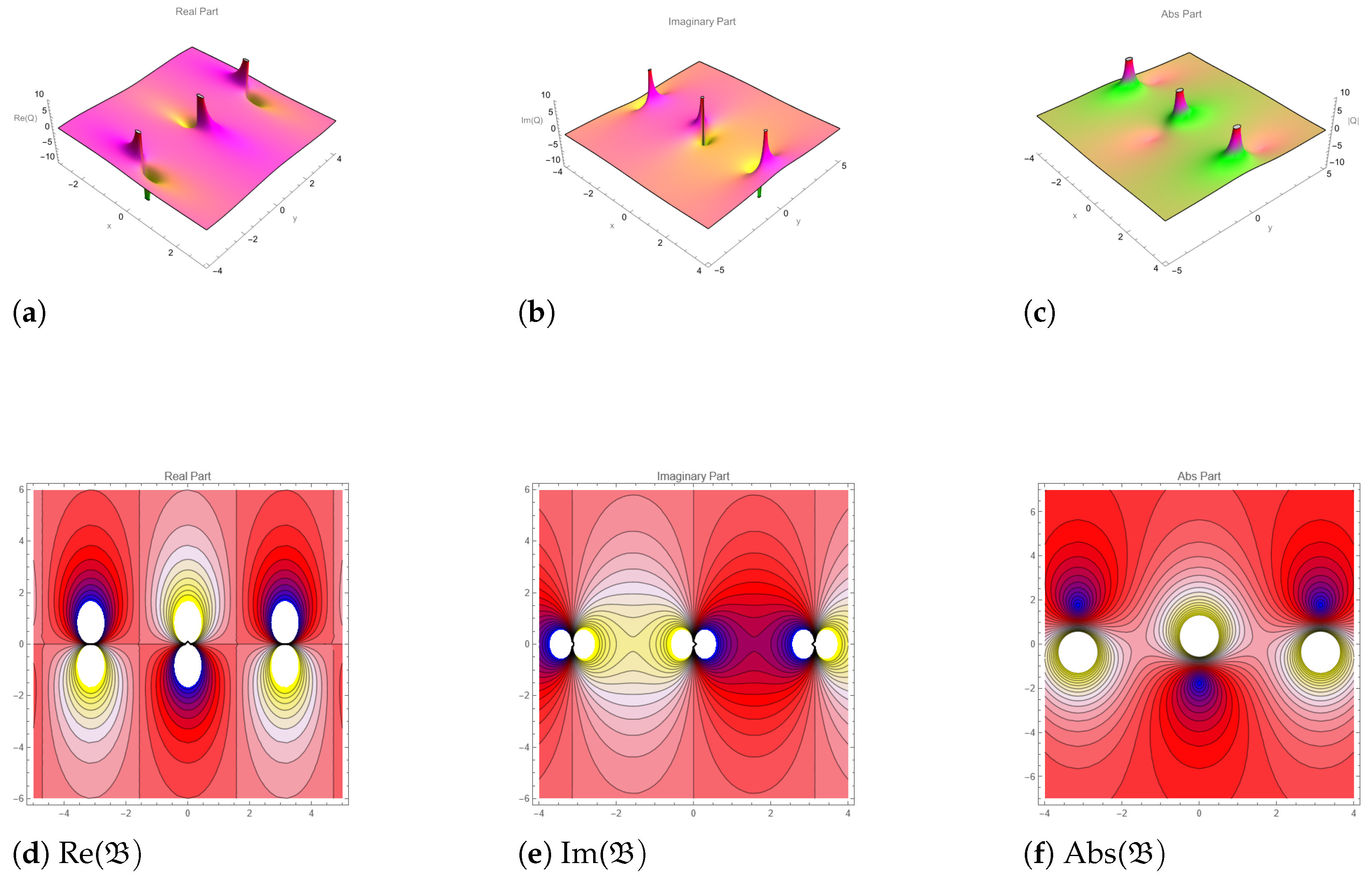
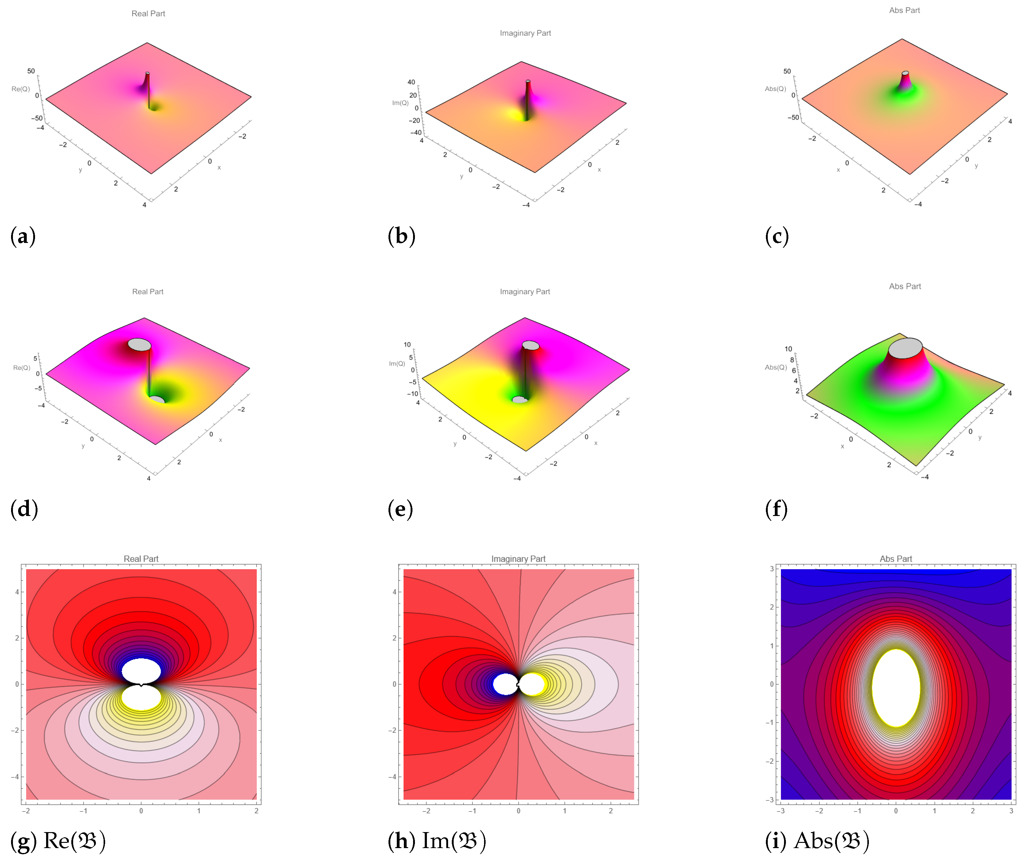
5. Graphical Representation

The pictorial appearance of the solutions produced is investigated in this section. Specific values are supplied to the unknown constants to construct 3D and contour graphs of the resulting solutions. The figures depicted in part (a) reflect a real 3D plot of the results, while part (b) represents the imaginary 3D plot of the solutions, part (c) displays the absolute 3D graph of solutions, part (d) depicts the real contour plot of solutions, part (e) displays the imaginary contour plot of solutions, and part (f) represents the absolute contour plot of the solutions. Figure 1 illustrates the lump solitary wave with varying values of constants ${\Phi }_1(t,y,x):\alpha =1,$ ${\beta }_1=0,{\delta }_1=i,\rho =1,\theta =i,\xi =\theta x+\rho t$, with t = [−4,4]. Figure 2 lumps the solitary wave with varying values of constants ${\Phi }_2(t,y,x):{\beta }_1=0,{\delta }_1=-4i,\rho =-0.4i,\theta =1.3,$ $\xi =\theta x+\rho t$, with t = [−4,4]. Figure 3 represents the lump solitary wave with varying values of constants ${\Phi }_5(t,y,x):\alpha =1,{\delta }_1=-i,\rho =0.5i,\theta =1,\xi =\theta x+\rho t$, with t = [−4,4]. Figure 4 represents the lump solitary wave with varying values of constants ${\Phi }_6(t,y,x):\alpha =1,{\beta }_1=0.02$, ${\delta }_1=3i,$ $\rho =0.3i,\theta =0.5,\xi =\theta x+\rho t$, with t = [−4,4]. Figure 5 represents the lump solitary wave with varying values of constants ${\Phi }_{13}(t,y,x):\alpha =i,{\beta }_1=0,{\delta }_1=-i,\rho =-2i,\theta =2,$ $\xi =\theta x+\rho t$, with t = [−4,4]. Figure 6 indicates the lump solitary wave with varying values of constants ${\Phi }_{17}(t,y,x):\alpha =2i,{\delta }_1=i,\rho =-1,\theta =i,\xi =\theta x+\rho t$, with t = [−4,4].

6. Conclusions

The fundamental purpose of the research that was carried out was to investigate the generalized $(1+1)$-dimensional Kundu–Eckhaus equation, which is a nonlinear partial differential equation that includes a dispersion term in addition to the original one. This equation is typically utilized to model the transmission of femtosecond pulses over the length of an optical fiber. The multivariate generalized exponential rational integral function approach has been utilized because of its adaptability. As a direct consequence, a large variety of localized waves have been discovered. To make the process of physically interpreting these solutions easier, several of them have been depicted in figures, such as $3D$, $2D$, and contour plots, using appropriate parameters. The results of this research shed light on the stability features of the equation as well as its behavior under various circumstances. The plots provide a means of graphically representing the intricate behavior of the equation and assisting in interpreting the findings. This method has the potential to produce fresh insights and a deeper understanding of these equations. Researchers can improve their comprehension of the behavior of nonlinear systems and phenomena if they use the aforementioned strategies.

References

1. Sonmezoglu, A. Stationary optical solitons having Kudryashov’s quintuple power law nonlinearity by extended G G 2 –expansion. Optik 2022, 253, 168521. [Google Scholar] [CrossRef]
2. Rezazadeh, H.; Davodi, A.G.; Gholami, D. Combined formal periodic wave-like and soliton-like solutions of the conformable Schrödinger-KdV equation using the G G -expansion technique. Result Phys. 2023, 47, 106352. [Google Scholar] [CrossRef]
3. Wang, M.Y.; Biswas, A.; Yıldırım, Y.; Moraru, L.; Moldovanu, S.; Alshehri, H.M. Optical solitons for a concatenation model by Trial equation approach. Electronics 2023, 12, 19. [Google Scholar] [CrossRef]
4. Ekici, M.; Sonmezoglu, A. Optical solitons with Biswas-Arshed equation by extended trial function method. Optik 2019, 177, 13–20. [Google Scholar] [CrossRef]
5. Pandir, Y.; Gurefe, Y.; Misirli, E. The extended trial equation method for some time fractional differential equations. Discret. Dyn. Nat. Soc. 2013, 2013, 491359. [Google Scholar] [CrossRef]
6. Zheng, B. The Riccati Sub-ODE method for fractional differential-difference equations. WSEAS Trans. Math. 2014, 13, 192–200. [Google Scholar]
7. Akinyemi, L.; Mirzazadeh, M.; Amin, B.S.; Hosseini, K. Dynamical solitons for the perturbated Biswas–Milovic equation with Kudryashov’s law of refractive index using the first integral method. J. Mod. Opt 2022, 69, 172–182. [Google Scholar] [CrossRef]
8. Ilie, M. An application of the first integral method for the time-fractional differential equation. J. Food Compos. Anal. 2022, 13, 32–44. [Google Scholar]
9. Yao, S.W.; Manzoor, R.; Zafar, A.; Inc, M.; Abbagari, S.; Houwe, A. Exact soliton solutions to the Cahn–Allen equation and Predator–Prey model with truncated M-fractional derivative. Result Phys. 2022, 37, 105455. [Google Scholar] [CrossRef]
10. Ibrahim, S.; Ashir, A.M.; Sabawi, Y.A.; Baleanu, D. Realization of optical solitons from nonlinear Schrödinger equation using modified Sardar sub-equation technique. Opt. Quantum Electron. 2023, 55, 617. [Google Scholar] [CrossRef]
11. Cinar, M.; Secer, A.; Ozisik, M.; Bayram, M. Derivation of optical solitons of dimensionless Fokas-Lenells equation with perturbation term using Sardar sub-equation method. Opt. Quantum Electron. 2022, 54, 402. [Google Scholar] [CrossRef]
12. Zayed, E.M.E. A note on the modified simple equation method applied to Sharma–Tasso–Olver equation. Appl. Math. Comput. 2011, 218, 3962–3964. [Google Scholar] [CrossRef]
13. Kaplan, M.; Bekir, A.; Akbulut, A.; Aksoy, E. The modified simple equation method for nonlinear fractional differential equations. Rom. J. Phys. 2015, 60, 1374–1383. [Google Scholar]
14. Ekici, M. Optical solitons with Kudryashov’s quintuple power–law coupled with the dual form of non–local law of refractive index with extended Jacobi’s elliptic function. Opt. Quantum Electron. 2022, 54, 279. [Google Scholar] [CrossRef]
15. Khalil, T.A.; Badra, N.; Ahmed, H.M.; Rabie, W.B. Optical solitons and other solutions for coupled system of nonlinear Biswas–Milovic equation with Kudryashov’s law of refractive index by Jacobi elliptic function expansion method. Optik 2022, 253, 168540. [Google Scholar] [CrossRef]
16. Ekici, M. Stationary optical solitons with Kudryashovs quintuple power law nonlinearity by extended Jacobi’s elliptic function expansion. J. Nonlinear Opt. Phys. Mater. 2023, 32, 2350008. [Google Scholar] [CrossRef]
17. Mandal, U.K.; Malik, S.; Kumar, S.; Zhang, Y.; Das, A. Integrability aspects, rational type solutions and invariant solutions of an extended (3+ 1)-dimensional B-type Kadomtsev–Petviashvili equation. Chaos Solitons Fractals 2024, 181, 114689. [Google Scholar] [CrossRef]
18. Malik, S.; Kumar, S.; Biswas, A.; Yıldırım, Y.; Moraru, L.; Moldovanu, S.; Iticescu, C.; Moshokoa, S.P.; Bibicu, D.; Alotaibi, A. Gap solitons in fiber Bragg gratings having polynomial law of nonlinear refractive index and cubic–quartic dispersive reflectivity by lie symmetry. Symmetry 2023, 15, 963. [Google Scholar] [CrossRef]
19. Ahmed, M.S.; Zaghrout, A.S.; Ahmed, H.M.; Arnous, A.H. Optical soliton perturbation of the Gerdjikov–Ivanov equation with spatio-temporal dispersion using a modified extended direct algebraic method. Optik 2022, 259, 168904. [Google Scholar] [CrossRef]
20. Ghayad, M.S.; Badra, N.M.; Ahmed, H.M.; Rabie, W.B. Derivation of optical solitons and other solutions for nonlinear Schrödinger equation using modified extended direct algebraic method. Alex. Eng. J. 2023, 64, 801–811. [Google Scholar] [CrossRef]
21. Zhang, X.; Ren, B. Resonance solitons, soliton molecules and hybrid solutions for a (2+1)-dimensional nonlinear wave equation arising in the shallow water wave. Nonlinear Dyn. 2024, 112, 4793–4802. [Google Scholar] [CrossRef]
22. Yang, X.; Zhang, Y.; Li, W. General high-order solitons and breathers with a periodic wave background in the nonlocal Hirota-Maccari equation. Nonlinear Dyn. 2024, 112, 4803–4813. [Google Scholar] [CrossRef]
23. Wu, J. Riemann-Hilbert approach and soliton analysis of a novel nonlocal reverse-time nonlinear Schrödinger equation. Nonlinear Dyn. 2024, 112, 4749–4760. [Google Scholar] [CrossRef]
24. Kumar, S.; Malik, S. The (3+ 1)-dimensional Benjamin–Ono equation: Painlevé analysis, rogue waves, breather waves and soliton solutions. Int. J. Mod. Phys. B 2022, 36, 2250119. [Google Scholar] [CrossRef]
25. Shen, Y.; Tian, B.; Cheng, C.D.; Zhou, T.Y. N-soliton, M th-order breather, H th-order lump, and hybrid solutions of an extended (3+1)-dimensional Kadomtsev-Petviashvili equation. Nonlinear Dyn. 2023, 111, 10407–10424. [Google Scholar] [CrossRef]
26. Rao, J.; Mihalache, D.; Cheng, Y.; He, J. Lump-soliton solutions to the Fokas system. Phys. Lett. A 2019, 383, 1138–1142. [Google Scholar] [CrossRef]
27. Kumar, S.; Malik, S.; Rezazadeh, H.; Akinyemi, L. The integrable Boussinesq equation and it’s breather, lump and soliton solutions. Nonlinear Dyn. 2022, 107, 2703–2716. [Google Scholar] [CrossRef]
28. Hussain, E.; Li, Z.; Shah, S.; Zo’bi, E.; Hussien, M. Dynamics study of stability analysis, sensitivity insights and precise soliton solutions of the nonlinear (STO)-Burger equation. Opt. Quantum Electron. 2023, 55, 1274. [Google Scholar] [CrossRef]
29. Hussain, E.; Shah, S.A.A.; Bariq, A.; Li, Z.; Ahmad, M.R.; Ragab, A.E.; Az-Zo’bi, E.A. Solitonic solutions and stability analysis of Benjamin Bona Mahony Burger equation using two versatile techniques. Sci. Rep. 2024, 14, 13520. [Google Scholar] [CrossRef]
30. Khater, M.M.A. Nonparaxial pulse propagation in a planar waveguide with Kerr–like and quintic nonlinearities; computational simulations. Chaos Soliton Fractals 2022, 157, 111970. [Google Scholar] [CrossRef]
31. Xia, T.; Chen, X.; Chen, D. Darboux transformation and soliton-like solutions of nonlinear Schroedinger equations. Chaos Soliton Fractals 2005, 26, 889–896. [Google Scholar] [CrossRef]
32. Jing, Z.; Yang, J.; Feng, W. Bifurcation and chaos in neural excitable system. Chaos Soliton Fractals 2006, 27, 197–215. [Google Scholar] [CrossRef]
33. Li, Z.; Hussain, E. Qualitative analysis and optical solitons for the (1+ 1)-dimensional Biswas-Milovic equation with parabolic law and nonlocal nonlinearity. Results Phys. 2024, 56, 107304. [Google Scholar] [CrossRef]
34. Beenish; Hussain, E.; Younas, U.; Tapdigoglu, R.; Garayev, M. Exploring Bifurcation, Quasi-Periodic Patterns, and Wave Dynamics in an Extended Calogero-Bogoyavlenskii-Schiff Model with Sensitivity Analysis. Int. J. Theor. Phys. 2025, 64, 146. [Google Scholar] [CrossRef]
35. Li, Z.; Hussain, E. Qualitative analysis and traveling wave solutions of a (3+1)-dimensional generalized nonlinear Konopelchenko-Dubrovsky-Kaup-Kupershmidt system. Fractal Fract. 2025, 9, 285. [Google Scholar] [CrossRef]
36. Beenish; Samreen, M. Bifurcation, Multistability, and Soliton Dynamics in the Stochastic Potential Korteweg-de Vries Equation. Int. J. Theor. Phys. 2025, 64, 1–22. [Google Scholar] [CrossRef]
37. Yao, S.W.; Behera, S.; Inc, M.; Rezazadeh, H.; Virdi, J.P.S.; Mahmoud, W.; Arqub, O.A.; Osman, M.S. Analytical solutions of conformable Drinfeld–Sokolov–Wilson and Boiti Leon Pempinelli equations via sine–cosine method. Result Phys. 2022, 42, 105990. [Google Scholar] [CrossRef]
38. Fendzi-Donfack, E.; Temgoua, G.W.K.; Djoufack, Z.I.; Kenfack-Jiotsa, A.; Nguenang, J.P.; Nana, L. Exotical solitons for an intrinsic fractional circuit using the sine-cosine method. Chaos Soliton Fractals 2022, 160, 112253. [Google Scholar] [CrossRef]
39. Hussain, E.; Shah, S.A.A.; Rafiq, M.N.; Ragab, A.E.; Az-Zo’bi, E.A. Exact solutions and modulation instability analysis of a generalized Kundu-Eckhaus equation with extra-dispersion in optical fibers. Phys. Scr. 2024, 99, 055222. [Google Scholar] [CrossRef]
40. Niwas, M.; Kumar, S.; Rajput, R.; Chadha, D. Exploring localized waves and different dynamics of solitons in (2+ 1)-dimensional Hirota bilinear equation: A multivariate generalized exponential rational integral function approach. Nonlinear Dyn. 2024, 1–14. [Google Scholar] [CrossRef]
41. Younas, U.; Hussain, E.; Muhammad, J.; Sharaf, M.; Meligy, M.E. Chaotic Structure, Sensitivity Analysis and Dynamics of Solitons to the Nonlinear Fractional Longitudinal Wave Equation. Int. J. Theor. Phys. 2025, 64, 42. [Google Scholar] [CrossRef]
42. Muhammad, J.; Younas, U.; Nasreen, N.; Khan, A.; Abdeljawad, T. Multicomponent nonlinear fractional Schrödinger equation: On the study of optical wave propagation in the fiber optics. Partial. Differ. Equ. Appl. Math. 2024, 11, 100805. [Google Scholar] [CrossRef]
43. Ajmal, M.; Muhammad, J.; Younas, U.; Hussian, E.; El-Meligy, M.; Sharaf, M. Exploring the Gross-Pitaevskii Model in Bose-Einstein Condensates and Communication Systems: Features of Solitary Waves and Dynamical Analysis. Int. J. Theor. Phys. 2025, 64, 1–26. [Google Scholar] [CrossRef]
44. Ahmed, K.K.; Badra, N.M.; Ahmed, H.M.; Rabie, W.B. Soliton solutions of generalized Kundu-Eckhaus equation with an extra-dispersion via improved modified extended tanh-function technique. Opt. Quantum Electron. 2023, 55, 299. [Google Scholar] [CrossRef]
45. Hamza, A.E.; Suhail, M.; Alsulami, A.; Mustafa, A.; Aldwoah, K.; Saber, H. Exploring Soliton Solutions and Chaotic Dynamics in the (3+ 1)-Dimensional Wazwaz–Benjamin–Bona–Mahony Equation: A Generalized Rational Exponential Function Approach. Fractal Fract. 2024, 8, 592. [Google Scholar] [CrossRef]
46. Asghari, Y.; Eslami, M.; Matinfar, M.; Rezazadeh, H. Novel soliton solution of discrete nonlinear Schrödinger system in nonlinear optical fiber. Alex. Eng. J. 2024, 90, 7–16. [Google Scholar] [CrossRef]
Figure 1. Pictorial representation of Equation (22): (a,d) real, (b,e) imaginary and (c,f) absolute components of the lump solitary wave with varying values of constants Φ 1 ( t , y , x ) : α = 1 , β 1 = 0 , δ 1 = i , ρ = 1 , θ = i , ξ = θ x + ρ t , with t = [−4,4].
Axioms 14 00513 g001
Figure 2. Pictorial representation of Equation (24): (a,d) real, (b,e) imaginary and (c,f) absolute components of lump solitary wave with varying values of constants Φ 2 ( t , y , x ) : β 1 = 0 , δ 1 = 4 i , ρ = 0.4 i , θ = 1.3 , ξ = θ x + ρ t , with t = [−4,4].
Axioms 14 00513 g002
Figure 3. Pictorial representation of Equation (32): (a,d) real, (b,e) imaginary and (c,f) absolute components of lump solitary wave with varying values of constants Φ 5 ( t , y , x ) : α = 1 , δ 1 = i , ρ = 0.5 i , θ = 1 ,   ξ = θ x + ρ t , with t = [−4,4].
Axioms 14 00513 g003
Figure 4. Pictorialrepresentation of Equation (34): (a,d) real, (b,e) imaginary and (c,f) absolute components across three rows of the lump solitary wave with varying values of constants Φ 6 ( t , y , x ) : α = 1 , β 1 = 0.02 , δ 1 = 3 i , ρ = 0.3 i , θ = 0.5 , ξ = θ x + ρ t , with t = [−4,4].
Axioms 14 00513 g004
Figure 5. Pictorial representation of Equation (52): (a,d) real, (b,e) imaginary and (c,f) absolute components of the lump solitary wave with varying values of constants Φ 13 ( t , y , x ) : α = i , β 1 = 0 , δ 1 = i , ρ = 2 i , θ = 2 , ξ = θ x + ρ t , with t = [−4,4].
Axioms 14 00513 g005
Figure 6. Pictorial representation of Equation (53): (a,d) real, (b,e) imaginary and (c,f) absolute components of the lump solitary wave with varying values of constants Φ 17 ( t , y , x ) : α = 2 i , δ 1 = i , ρ = 1 , θ = i , ξ = θ x + ρ t , with t = [−4,4].
Axioms 14 00513 g006
Disclaimer/Publisher’s Note: The statements, opinions and data contained in all publications are solely those of the individual author(s) and contributor(s) and not of MDPI and/or the editor(s). MDPI and/or the editor(s) disclaim responsibility for any injury to people or property resulting from any ideas, methods, instructions or products referred to in the content.