Existence and Global Exponential Stability of Equilibrium for an Epidemic Model with Piecewise Constant Argument of Generalized Type

Abstract

The authors investigate an epidemic model described by a differential equation, which includes a piecewise constant argument of the generalized type (DEPCAG). In this work, the main goal is to find an invariant region for the system and prove the existence and uniqueness of solutions with the defined conditions using integral equations. On top of that, an auxiliary result is established, outlining the relationship between the unknown function values in the deviation argument and the time parameter. The stability analysis is conducted using the Lyapunov–Razumikhin method, adapted for differential equations with a piecewise constant argument of the generalized type. The trivial equilibrium’s stability is examined, and the stability of the positive equilibrium is assessed by transforming it into a trivial form. Finally, sufficient conditions for the uniform asymptotic stability of both the trivial and positive equilibria are established.

1. Introduction

Differential equations serve as fundamental tools for modeling real-world phenomena, offering valuable insights into various scientific disciplines. In particular, population dynamics provide a mathematical framework for addressing biological challenges. Differential equations with deviating arguments are particularly relevant in this context, as time delays arising from biological factors can be captured and incorporated into epidemic models through such formulations. Constructing these models accurately with multi-dimensional dynamic analysis, as well as developing effective control strategies tailored to disease dynamics, is important for understanding and controlling diseases. Given the severity and probable consequences of future outbreaks, safeguarding public health necessitates a thorough study on the emerging properties of the mathematics of diseases. This understanding does not come easily and requires a significantly concentrated research effort. While identifying prominent parameters defining epidemic geometry is an important step, it is just as important to study the life span of these parameters since many factors associated with individuals and locales drive the rate of transmission. The history of a region greatly influences the current state of disease outbreak and therefore warrants the adoption of differential equations of deviating arguments. The qualitative theory of these types of equations offers one of the strongest means of verifying the behavior of epidemic models. Consequently, the development and refinement of models that accurately capture real-world processes have remained central to epidemiological research. Within this framework, the delayed SIS model,

$$y^{\prime }\left(t\right)=by(t-T)\left\{1-y\left(t\right)\right\}-cy\left(t\right),$$

(1)

proposed by Cooke [1] is particularly noteworthy. In this model, the parameters b and c represent the infection and recovery rates, respectively, and are assumed to be positive constants. The function $y\left(t\right)$ denotes the proportion of infectious individuals at time t, while $S\left(t\right)$ represents the proportion of susceptible individuals.

Cooke [1] assumes that $y\left(t\right)+S\left(t\right)=1$, suggesting that human infection confers negligible immunity and does not lead to mortality or isolation. Based on this assumption, it follows that a vector can transmit the infection to a susceptible human upon completion of the incubation period (see Cooke [1] and Huang et al. [2]). Furthermore, let $x\left(t\right)$ denote the number of infectious vectors in the population at time t, as introduced by Cooke [1]. The model categorizes the population into two groups—susceptible and infectious—under the assumption of homogeneous mixing between human and vector populations, a concept explored by Busenberg and Cooke [3]. According to Cooke [1], Equation (1), which incorporates a delay term, describes the proportion of infectious individuals while accounting for fundamental assumptions regarding the transmission dynamics of a communicable disease.

(i)

Infection is transmitted from vectors, such as mosquitoes, to humans.

(ii)

Infected individuals acquire immunity but do not experience mortality or isolation.

(iii)

The total population remains constant, with no changes due to birth, death, or migration.

(iv)

After a susceptible vector acquires the infection from an infected human, a fixed incubation period, T, is required for the pathogen to develop, after which the vector becomes capable of transmitting the infection.

(v)

The model assumes homogeneous mixing between human and vector populations.

(vi)

The recovery rate of infected individuals is represented by a positive constant, c.

(vii)

The vector population is sufficiently large, and $x\left(t\right)$ is proportional to $y(t-T)$.

(viii)

Disease transmission occurs exclusively from vectors, such as mosquitoes, to humans.

Under these assumptions, the term $S\left(t\right)x\left(t\right)$ denotes the rate at which new infections occur per unit time. As a result, the evolution of the proportion of infected individuals within the population is dictated by the differential Equation (1) (Cooke, 1979 [1]).

Epidemic models incur time-associated delays because of several factors like incubating time, medical response to cases, and behavior alterations. These time-associated components can affect equilibrium conditions, which might cause periodic resurgences or completely extinguish subdued stable lazy states (Abta et al., 2020 [4]). Prior works have shown that delays have a significant impact on the dynamics of disease spread (Liu et al., 2013 [5]). Therefore, a meticulous investigation regarding the rest point or equilibrium analysis is necessary to determine whether the infection becomes chronic or gets eradicated.

A good number of studies have studied the impact of time delays concerning the model fitting frames in Susceptible–Infected–Susceptible (SIS) models. Ramesh and Ravindra (2024) [6] studied Hopf bifurcations in the context of a delayed SIS and pointed out how delay parameters can remarkably contribute to infectious disease persisting. Likewise, Lamrani Alaoui et al. (2022) [7] studied a diffusive SEIR model with distributed delay, focusing on the effect of spatial and temporal factors combined. These studies underscore the importance of understanding delay-induced phenomena to develop effective deflection processes.

Lyapunov functionals and characteristic equations are often employed in the context of stability analyses for delayed SIS models (Agaba et al., 2017 [8]). In Ghosh et al.’s study (2022) [9], it was shown that the stability conditions are affected by both the amount of delay and the basic reproduction number ($R_0$). Specifically, when $R_0$ remains below a critical threshold, the system maintains a stable disease-free equilibrium; however, once $R_0$ exceeds this threshold, the dynamics transition to an endemic equilibrium.

The dynamics pertaining to the spread of the disease are significantly influenced by the behavioral responses. The incorporation of time-dependent behavioral changes, such as elevated precautionary activities during outbreak periods, markedly changes the system’s stability. Such considerations are important for infectious diseases like COVID-19, where the level of public attention and government policies fluctuate over time (Zhao et al., 2020 [10]).

Delayed SIS models possess significant theoretical and practical relevance in epidemiology. In their study, Wang and Ruan (2017) [11] analyzed nosocomial infections, with particular emphasis on the impact of environmental factors related to treatment delays and hospital contamination. Their findings indicate that incorporating dynamic delay components into the analysis improves the accuracy of infection control strategies.

A significant portion of the literature has dealt with the global stability properties of SIS models. Li and Ma [12], in their study from 2004, investigated the effects of variable population size with parametric bounds and posited some conditions under which disease presence is ensured. Xu and Ma (2009) [13] built upon this primary work by adding the nonlinear incidence rate, which improved the model’s ability to portray complex transmission dynamics.

The consequences of spatial heterogeneity seem to have become a popular topic to study. Wang et al. (2012) [14] and Yang et al. (2011) [15] studied the addition of reaction–diffusion processes to SIS models and showed how both the spatial and temporal components of an epidemic affect its threshold. These outcomes hint towards the greater accuracy of temporal and spatial epidemiological models when both dimensions are considered.

The incorporation of imprecise stochastic elements tends to increase the complexity of delayed SIS models. Xu and Chen (2017) [16] studied the impact of random oscillations on SIS systems and showed that these stochastic shifts affect the stability condition significantly. This underlines the need to combine deterministic and stochastic components of disease modeling if one intends to enhance predictive precision.

Also, computer-based simulations validate the concepts hypothesized. Pao (1996, 2002) [17,18] revealed the long-term dynamics of delayed epidemic models using bifurcation analysis. It is now possible to predict the course of outbreaks and test the efficiency of many intervention methods by calculating the outbreak delay parameters.

Recent developments in modeling have introduced a new class of systems that integrate the characteristics of both continuous-time and discrete-time frameworks. This hybrid approach effectively captures the abrupt qualitative changes observed in continuous-time dynamics; see [19,20,21,22,23,24,25,26,27,28]. The systematic study of mathematical models incorporating piecewise constant arguments was initially motivated by applications in biomedical research. These models share structural similarities with certain sequential–continuous formulations in disease dynamics; see [29].

The rigorous theoretical and applied investigation of piecewise constant systems began in the early 1980s. Since then, differential equations involving piecewise constant functions or variables have drawn significant interest from researchers in mathematics and various applied sciences. Many real-world phenomena can be effectively modeled using such systems, where the corresponding differential equations include piecewise constant arguments (commonly referred to as DEPCAs). These systems are inherently discontinuous and often exhibit more complex and diverse behaviors compared to conventional continuous models governed by standard differential equations; see [26].

DEPCAs integrate aspects of both differential equations and differential–difference equations. In particular, differential equations with piecewise constant delay (DEPCD) frequently arise in economics, biology, and physics, providing a more suitable framework than traditional delay differential equations for accurately capturing discrete and abrupt changes in dynamic processes. The concept of delay in these models accounts for system memory, where past states significantly influence present behavior. It is worth noting that research within the mathematical community on generalized types of DEPCAs remains relatively limited; see [19,23,24,30,31,32,33,34,35].

Classical SIS models with delays usually assume continuous or fixed delay structures. However, such assumptions may not reflect real-time discontinuous responses, such as lockdowns or behavioral shifts. The DEPCA formulation offers a flexible alternative by capturing intervals with advanced (anticipatory) and retarded (delayed) arguments, offering a more granular reflection of behavioral and administrative responses in epidemics. A variety of extensions of classical SIS models have been proposed to better reflect complex real-world epidemic behavior. Fractional-order SIS models capture memory effects and anomalous diffusion, as seen in [36,37]. Stochastic and hybrid SIS models address randomness and external shocks in infection dynamics [38,39,40]. Time delays are incorporated to model incubation or response lags [41,42]. Moreover, SIS models on complex or multilayer networks have been developed to represent realistic social or contact structures, sometimes with adaptive transmission or optimal control strategies [43,44,45,46]. Spatial heterogeneity and human mobility have been addressed via reaction–diffusion systems and dimension reduction techniques [47,48,49]. Recent efforts also involve control-oriented modeling with saturation, vaccination, and feedback policy design [39,50]. In addition, qualitative analyses of SIS models continue to evolve. Studies such as [37,51] explore long-term stability and bifurcation phenomena, while others examine equilibrium sensitivity, treatment saturation, and behavior-driven dynamics. These works provide a robust foundation for SIS modeling but often remain limited to systems with fixed delays or fully continuous dynamics. Few consider analytical structures such as piecewise constant-deviated arguments with both advanced and retarded behaviors.

Building on this foundation, the primary objective of this paper is to establish sufficient conditions for the existence, uniqueness, and stability of a positive equilibrium in an epidemic model incorporating a piecewise constant argument of the generalized type.

Denote by $\mathbb{N}$ and ${\mathbb{R}}^{+}$ the sets of natural numbers and positive real numbers, respectively. Consider two real-valued sequences, $t_m$ and ${\gamma }_m$, indexed by $m\in \mathbb{N}$, satisfying $t_m<t_{m+1}$ and $t_m\le {\gamma }_m\le t_{m+1}$ for all m. Assume the existence of a constant $\widehat{\theta }>0$ such that $t_{m+1}-t_m\le \widehat{\theta }$ for every $m\in \mathbb{N}$. Additionally, suppose that $t_m\to \infty$ as $m\to \infty$. Define the piecewise constant function $\gamma :\mathbb{R}\to \mathbb{R}$ by setting $\gamma \left(t\right)={\gamma }_m$ for $t\in I_m=[t_m,t_{m+1})$, with ${\theta }_m^{+}={\gamma }_m-t_m$, ${\theta }_m^{-}=t_{m+1}-{\gamma }_m$ and $t_{m+1}-t_m={\theta }_m^{+}+{\theta }_m^{-}$. The parameters ${\theta }_m^{+}$ and ${\theta }_m^{-}$ represent the lengths of the advanced and delayed subintervals, respectively.

The proposed model with the DEPCAG is given by

$$y^{\prime }\left(t\right)=by\left(\gamma \left(t\right)\right)\{1-y\left(t\right)\}-cy\left(t\right),$$

(2)

where $t,b,c\in {\mathbb{R}}^{+}$, and $\gamma \left(t\right)={\gamma }_m$ if $t_m\le t<t_{m+1}$, $m\in \mathbb{N}$.

In epidemiological terms, the parameter b represents the average number of secondary infections caused by one infected individual per unit time, while c reflects the rate at which infected individuals recover or are removed from the infectious pool. The deviation function $\gamma \left(t\right)$ models delays or advances in the system, corresponding to time-lagged effects such as incubation periods, symptom recognition, or the influence of public health interventions that anticipate outbreaks.

This formulation extends the DEPCAG approach to enhance our understanding of epidemic dynamics across various models.

To clarify why the epidemic model (2) is classified as an alternately advanced and retarded type, we observe that the argument’s deviation character varies throughout the system’s evolution. Specifically, the argument is considered deviated when it either advances or lags behind.

Fix $m\in \mathbb{N}$ and examine the system (2) over the interval $I_m=[t_m,t_{m+1})$. Within this interval, the identification function $\gamma \left(t\right)$ takes the constant value ${\gamma }_m$. If $t\in I_m^{+}=[t_m,{\gamma }_m)$, then $\gamma \left(t\right)\ge t$, meaning that the system (2) behaves as an equation with an advanced argument. Conversely, if $t\in I_m^{-}=({\gamma }_m,t_{m+1})$, then $\gamma \left(t\right)<t$, indicating that the epidemic model (2) follows a retarded argument formulation.

As a result, the model (2) alternates between advanced and retarded argument types throughout its progression. In other words, the deviation nature of the argument shifts dynamically over time, classifying the epidemic model (2) as an alternately advanced and retarded system.

Mathematical models frequently incorporate retarded arguments to account for the influence of past states on the dynamics of the present system. By integrating such historical dependencies, these models can more accurately capture temporal effects, offering a vivid representation of how prior conditions shape the evolution of future behavior. This approach is particularly crucial in systems governed by delay differential equations, control theory, and physical phenomena such as electromagnetic wave propagation.

In practical applications, historical effects play a pivotal role across various disciplines, including biological systems and engineering processes, where time delays significantly impact system stability and performance. Consequently, the careful selection of retarded arguments is essential for constructing precise and predictive models.

Conversely, the introduction of an advanced argument endows models with predictive capabilities, enabling them to characterize how future states influence present dynamics. Although this formulation challenges conventional causal frameworks, it has found extensive applications in time-symmetric physics, predictive control mechanisms, and optimization strategies—particularly in decision-making processes that require anticipatory adjustments. Incorporating future dependencies into models enhances their ability to simulate decision-making processes while offering a more refined depiction of deterministic factors and complex feedback structures within dynamic systems.

Real-world examples such as periodic lockdown schedules, alternating school closures, or cyclic testing protocols represent policy-based interventions with abrupt transitions that naturally lead to piecewise constant behaviors in the system. These features motivate the use of the DEPCAG framework.

This study simultaneously considers both retarded and advanced arguments, extending the applicability of traditional models by developing a comprehensive framework that accommodates both historical dependencies and predictive effects. This dual approach not only deepens our understanding of the interplay between past influences and future expectations but also advances the refinement of mathematical modeling methodologies.

Although many studies exist on classical delay differential equations and even some on DEPCAG systems, few address alternately advanced and retarded arguments. Our work fills this gap by exploring equilibrium stability under a DEPCAG framework with these hybrid argument types, which are increasingly relevant in modeling adaptive epidemic responses.

This is the first paper, to the best of our knowledge, that examines the equilibrium of an epidemic model with piecewise alternately advanced and retarded arguments of a generalized type. With the help of linearization techniques with changes in coordinates, Banach’s fixed-point theorem, the Lyapunov–Razumikhin method, and Gronewald integral inequalities specialized for DEPCAG, a thorough analysis of stability is performed. Surprisingly, this approach mitigates the need for extensive calculations when compared to traditional methods, thereby streamlining methodologies for analysis and enhancing the precision of the results. As a result, the framework of integral inequalities presented by Pinto in 2009 [33] is strikingly effective for the analysis of complex models amidst sharp discontinuities.

The primary objective of this study is to investigate the stability of both trivial and positive equilibria in the epidemic model (2), incorporating a generalized piecewise constant argument. The paper is organized as follows:

In Section 2, we establish preliminary results that are fundamental for proving the existence and stability of solutions to the epidemic model with DEPCAG. In particular, we introduce a DEPCAG Gronwall-type inequality, which serves as a key analytical tool in our study. Section 3 explores the positive invariance of solutions in the epidemic model (2), thereby defining the invariant region associated with the solutions of the epidemic model (3). In Section 4, we derive essential auxiliary results for the epidemic model with DEPCAG, including Lemmas 3 and 5. These results clarify the relationship between the values of the unknown function at the deviation argument $\gamma \left(t\right)$ and its corresponding values at any given time t. Section 5 focuses on establishing sufficient conditions for the existence and uniqueness of solutions to the epidemic model by reformulating the problem in terms of integral equations. In Section 6, we analyze the stability of both the trivial and positive equilibria of the epidemic model (2) with DEPCAG using the Lyapunov–Razumikhin method. This section presents Theorems 3 and 4, which provide sufficient conditions for uniform asymptotic stability. These stability results, derived based on specific model parameters, offer theoretical insights into the long-term behavior of the epidemic model. Finally, Section 7 presents two illustrative examples along with numerical simulations to demonstrate the validity and applicability of the theoretical results.

2. Preliminaries and Definition

This section presents fundamental results essential for analyzing the existence and stability of the epidemic model with DEPCAG (2).

Let $I_i=[t_i,t_{i+1})$ denote the subintervals of ${\mathbb{R}}^{+}$, where ${\mathbb{R}}^{+}={\bigcup }_{i\in \mathbb{N}}{I}_i=[0,\infty )$. For each $t\in {\mathbb{R}}^{+}$, define $i=i\left(t\right)\in \mathbb{N}$ as the unique index such that $t\in I_i$.

To facilitate the analysis, we introduce the fundamental assumption.

Existence condition:

$${\rho }_i^{+}=(2b+c)({\gamma }_i-t_i)\le \underset{i\in \mathbb{N}}{sup}{\rho }_i^{+}=\rho <1,$$

where b and c are positive constants.

It is evident that Equation (2) has a trivial equilibrium at $y^{*}=0$ and a positive equilibrium at $y^{*}=1-c/b$, provided that $c<b$. By introducing the transformation $z=y-y^{*}$, the positive equilibrium is shifted to the trivial equilibrium, yielding the transformed equation:

$$z^{\prime }\left(t\right)=-bz\left(t\right)\left[1+z\left(\gamma \right(t\left)\right)\right]+cz\left(\gamma \left(t\right)\right).$$

(3)

Next, we define the following function classes, which will be utilized in the stability analysis:

$$\mathbb{K}=\left\{a\in C({\mathbb{R}}^{+},{\mathbb{R}}^{+}):a\mathrm{is}\mathrm{strictly}\mathrm{increasing}\mathrm{and}a\left(0\right)=0\right\},$$

$$\mathbb{M}=\left\{d\in C({\mathbb{R}}^{+},{\mathbb{R}}^{+}):d\left(0\right)=0,d\left(s\right)>0\mathrm{for}s>0\right\}.$$

To investigate the existence and uniqueness of solutions to the DEPCAG model (2), we adopt the following definition, adapted from [19,21,24,32,33].

Definition 1.

A function y is said to be a solution of the DEPCAG (2) on ${\mathbb{R}}^{+}=[0,\infty )$ if it satisfies the following conditions:

(i) 

y is continuous on ${\mathbb{R}}^{+}$.

(ii) 

The derivative $y^{\prime }\left(t\right)$ exists for all $t\in {\mathbb{R}}^{+}$, except possibly at points $t_i\in {\mathbb{R}}^{+}$, where $i\in \mathbb{N}$. At these points, one-sided derivatives exist.

(iii) 

The DEPCAG (2) holds for y on each interval $\left(t_i,t_{i+1}\right)$, where $i\in \mathbb{N}$, and it is also satisfied in terms of the right-hand derivative at points $t_i$, $i\in \mathbb{N}.$

To study the DEPCAG framework, we adopt the approach proposed by M. Pinto in [33], which is based on constructing an equivalent integral equation.

Proposition 1.

Let $(\tau ,y_0)\in {\mathbb{R}}^{+}\times {\mathbb{R}}^{+}.$ The function $y\left(t\right)=y(t,\tau ,y_0)$ is a solution of the epidemic model (2) on ${\mathbb{R}}^{+}$ in the sense of Definition 1 if and only if it satisfies the integral equation:

$$y\left(t\right)=e^{-c(t-\tau )}y\left(\tau \right)+{\int }_{\tau }^t{e}^{-c(t-s)}by\left(\gamma \left(s\right)\right)(1-y\left(s\right))ds,t\in {\mathbb{R}}^{+}.$$

(4)

Proof. 

Necessity: Consider the interval $I_{n-1}=[t_{n-1},t_n)$.

Integrating the epidemic model (2) over this interval yields

$$y\left(t\right)=e^{-c(t-t_{n-1})}y\left(t_{n-1}\right)+{\int }_{t_{n-1}}^t{e}^{-c(t-s)}by\left(\gamma \left(s\right)\right)(1-y\left(s\right))ds.$$

(5)

Since $\gamma \left(t\right)={\gamma }_{n-1}$ for all $t\in I_{n-1}=[t_{n-1},t_n)$, evaluating at $t=t_n$ gives

$$y\left(t_n\right)=e^{-c(t_n-t_{n-1})}y\left(t_{n-1}\right)+{\int }_{t_{n-1}}^{t_n}{e}^{-c(t_n-s)}by\left({\gamma }_{n-1}\right)(1-y\left(s\right))ds.$$

Similarly, for $t=t_{i\left(\tau \right)+1}$, we obtain

$$y\left(t_{i\left(\tau \right)+1}\right)=e^{-c(t_{i\left(\tau \right)+1}-\tau )}y\left(\tau \right)+{\int }_{\tau }^{t_{i\left(\tau \right)+1}}{e}^{-c(t_{i\left(\tau \right)+1}-s)}by\left({\gamma }_{i\left(\tau \right)}\right)(1-y\left(s\right))ds.$$

Solving the finite difference equation iteratively, we arrive at

$$\begin{array}{cc}\hfill y\left(t_n\right)=e^{-c(t_n-\tau )}y\left(\tau \right)& +{\int }_{\tau }^{t_{i\left(\tau \right)+1}}{e}^{-c(t_n-s)}by\left({\gamma }_{i\left(\tau \right)}\right)(1-y\left(s\right))ds\hfill \\ \hfill & +{\sum }_{k=i\left(\tau \right)+1}^{n-1}{\int }_{t_k}^{t_{k+1}}{e}^{-c(t_n-s)}by\left({\gamma }_k\right)(1-y\left(s\right))ds.\hfill \end{array}$$

Next, applying this result to (5) with $t\in I_{i\left(t\right)}$, we obtain

$$\begin{array}{cc}\hfill y\left(t\right)=e^{-c(t-\tau )}y\left(\tau \right)& +{\int }_{\tau }^{t_{i\left(\tau \right)+1}}{e}^{-c(t-s)}by\left({\gamma }_{i\left(\tau \right)}\right)(1-y\left(s\right))ds\hfill \\ \hfill & +{\sum }_{k=i\left(\tau \right)+1}^{n-1}{\int }_{t_k}^{t_{k+1}}{e}^{-c(t-s)}by\left({\gamma }_k\right)(1-y\left(s\right))ds\hfill \\ \hfill & +{\int }_{t_n}^t{e}^{-c(t-s)}by\left({\gamma }_n\right)(1-y\left(s\right))ds.\hfill \end{array}$$

By defining

$$\begin{array}{cc}\hfill {\int }_{\tau }^t{e}^{-c(t-s)}by\left(\gamma \left(s\right)\right)(1-y\left(s\right))ds=& {\int }_{\tau }^{t_{i\left(\tau \right)+1}}{e}^{-c(t-s)}by\left({\gamma }_{i\left(\tau \right)}\right)(1-y\left(s\right))ds\hfill \\ \hfill & +{\sum }_{k=i\left(\tau \right)+1}^{n-1}{\int }_{t_k}^{t_{k+1}}{e}^{-c(t-s)}by\left({\gamma }_k\right)(1-y\left(s\right))ds\hfill \\ \hfill & +{\int }_{t_n}^t{e}^{-c(t-s)}by\left({\gamma }_n\right)(1-y\left(s\right))ds\hfill \end{array}$$

and substituting it into the previous expression, we recover Equation (4), thereby completing the proof.

Sufficiency: Let $y\left(t\right)$ be a solution to the epidemic model (2) with DEPCAG. For a fixed $k\in \mathbb{N}$, consider the interval $I_k$. Differentiating Equation (4), we find that $y\left(t\right)$ satisfies the epidemic model (2) with DEPCAG. Taking the limit as $t\to t_k$ and noting that $y\left(\gamma \right(t\left)\right)$ is right-continuous, we conclude that $y\left(t\right)$ indeed satisfies the epidemic model (2) with DEPCAG over $I_k$. □

Remark 1.

By applying the same proof technique as in Proposition 1, the solution to the epidemic model (2) with DEPCAG can be expressed as

$$y\left(t\right)=y\left(\tau \right)+{\int }_{\tau }^t\left[by\left(\gamma \right(s\left)\right)(1-y(s\left)\right)-cy\left(s\right)\right]ds,t\in {\mathbb{R}}^{+}.$$

(6)

Next, we present the following lemma concerning a DEPCAG Gronwall-type integral inequality, similar to the result in [33], which serves as a fundamental auxiliary tool in this study. For the reader’s convenience, we provide the complete proof below.

Lemma 1.

Let $u:{\mathbb{R}}^{+}\to {\mathbb{R}}^{+}$ be a continuous function satisfying the inequality

$$u\left(t\right)\le u\left(\tau \right)+{\int }_{\tau }^t\left[{\mathcal{L}}_{1}u\left(s\right)+{\mathcal{L}}_{2}u\left(\gamma \left(s\right)\right)\right]ds.$$

(7)

Suppose that ${\mathcal{L}}_i$ (for $i=1,2$) are positive constants satisfying

$${\sigma }_i^{+}=\left({\mathcal{L}}_1+{\mathcal{L}}_2\right)({\gamma }_i-t_i)\le \underset{i\in \mathbb{N}}{sup}{\sigma }_i^{+}=\sigma <1, i\in \mathbb{N}.$$

(8)

Then, for $t\ge \tau$, the following inequalities hold:

$$u\left(t\right)\le u\left(\tau \right)exp\left(\left({\mathcal{L}}_1+{\displaystyle \frac{{\mathcal{L}}_2}{1-\sigma }}\right)(t-\tau )\right),$$

(9)

$$u\left(\gamma \left(t\right)\right)\le {\displaystyle \frac{u\left(\tau \right)}{1-\sigma }}exp\left(\left({\mathcal{L}}_1+{\displaystyle \frac{{\mathcal{L}}_2}{1-\sigma }}\right)(t-\tau )\right),$$

(10)

and

$$u\left({\gamma }_n\right)\le {\left(1-\sigma \right)}^{-1}u\left(t_n\right),n\ge i\left(\tau \right).$$

(11)

Proof. 

Define $v\left(t\right)$ as the right-hand side of inequality (7), so that

$$v\left(\tau \right)=u\left(\tau \right)+{\int }_{\tau }^{\tau }\left[{\mathcal{L}}_{1}u\left(s\right)+{\mathcal{L}}_{2}u\left(\gamma \left(s\right)\right)\right]ds=u\left(\tau \right).$$

Since $u\le v$ and v is a piecewise-differentiable and non-decreasing function, it satisfies the following differential inequality:

$$v^{\prime }\left(t\right)\le {\mathcal{L}}_{1}v\left(t\right)+{\mathcal{L}}_{2}v\left(\gamma \left(t\right)\right).$$

Integrating from r to t, we obtain

$$v\left(t\right)-v\left(r\right)\le {\int }_r^t\left[{\mathcal{L}}_{1}v\left(s\right)+{\mathcal{L}}_{2}v\left(\gamma \left(s\right)\right)\right]ds.$$

(12)

Setting $t={\gamma }_n$ and $r=t_n$ for $t\in [t_n,{\gamma }_n]$ and using the fact that v is non-decreasing, we obtain

$$\begin{array}{cc}\hfill v\left({\gamma }_n\right)& \le v\left(t_n\right)+{\int }_{t_n}^{{\gamma }_n}\left[{\mathcal{L}}_{1}v\left(s\right)+{\mathcal{L}}_{2}v\left(\gamma \left(s\right)\right)\right]ds\hfill \\ \hfill & \le v\left(t_n\right)+\left({\mathcal{L}}_1+{\mathcal{L}}_2\right)\left({\gamma }_n-t_n\right)v\left({\gamma }_n\right).\hfill \\ \hfill & \le v\left(t_n\right)+\sigma v\left({\gamma }_n\right).\hfill \end{array}$$

Applying the smallness condition (8), we conclude that

$$v\left({\gamma }_n\right)\le {\displaystyle \frac{v\left(t_n\right)}{1-\sigma }}.$$

Now, consider the particular case where $\tau =t_n$ in (7), which implies that $v\left(t_n\right)=u\left(t_n\right)$. Then, by applying condition (8), the estimate in (11) follows immediately.

For $t\in I_n$ and $r=t_n$ in (12), we obtain

$$\begin{array}{cc}\hfill v\left(t\right)& \le v\left(t_n\right)+{\int }_{t_n}^t\left[{\mathcal{L}}_{1}v\left(s\right)+{\mathcal{L}}_{2}v\left(\gamma \left(s\right)\right)\right]ds\hfill \\ \hfill & \le v\left(t_n\right)+{\int }_{t_n}^t\left[{\mathcal{L}}_{1}v\left(s\right)+{\mathcal{L}}_2{\displaystyle \frac{v\left(t_n\right)}{1-\vartheta }}\right]ds\hfill \\ \hfill & \le v\left(t_n\right)+\left({\mathcal{L}}_1+{\displaystyle \frac{{\mathcal{L}}_2}{1-\sigma }}\right){\int }_{t_n}^{t}v\left(s\right)ds,\hfill \end{array}$$

(13)

considering that v is a non-decreasing function. Then, by applying a DEPCAG Gronwall-type integral inequality to (13), we obtain the following estimate:

$$v\left(t\right)\le v\left(t_n\right)exp\left\{\left({\mathcal{L}}_1+{\displaystyle \frac{{\mathcal{L}}_2}{1-\sigma }}\right)(t-t_n)\right\}.$$

From this inequality, applying it recursively, we derive

$$v\left(t\right)\le v\left(\tau \right)exp\left\{\left({\mathcal{L}}_1+{\displaystyle \frac{{\mathcal{L}}_2}{1-\sigma }}\right)(t-\tau )\right\}.$$

Since $v\left(\tau \right)=u\left(\tau \right)$, and using $u\le v$ and (11), we obtain inequalities (9) and (10). □

3. Positive Invariance of Solutions to the Epidemic Model (2)

In this section, we analyze the positive invariance of solutions to the epidemic model (2). The following lemma and theorems establish the conditions under which the solutions remain within an invariant region. Specifically, these results provide insights into the invariance properties of the solutions to the epidemic model (3). We restrict our attention to solutions $y\left(t\right)$ satisfying the initial condition $0\le y\left(\tau \right)=y_0\le 1$ and define the admissible set as $\Omega =\{y\in {\mathbb{R}}^{+}:0\le y\le 1\}$.

Theorem 1.

If we have the initial conditions $y\left(\tau \right)\in \Omega$ and $b\le c$, then every solution $y\left(t\right)$ of the epidemic model (2) remains within Ω for all $t\ge \tau$; that is, Ω is positively invariant for the epidemic model (2) with DEPCAG.

Proof. 

Let $y:[\tau ,\infty )\to \mathbb{R}$ be a solution of the epidemic model (2) with DEPCAG satisfying the initial condition $0\le y\left(\tau \right)=y_0\le 1$. Then, the solution of the epidemic model (2) with DEPCAG is given by the following integral equation:

$$y\left(t\right)=e^{-c(t-\tau )}y\left(\tau \right)+{\int }_{\tau }^t{e}^{-c(t-s)}by\left(\gamma \left(s\right)\right)(1-y\left(s\right))ds,t\in [\tau ,\infty ).$$

Now, assume that $y\left(t\right)$ does not satisfy the inequality $0\le y\left(t\right)\le 1$ for $0\le \tau \le t<t_{k+1}$, where $k\in \mathbb{N}$. From the continuity of $y\left(t\right)$, there exists a maximal value $\mu$, with $0\le \tau \le \mu <t_{k+1}$, such that $0\le y\left(t\right)\le 1$ for all $0\le t\le \mu$, and one of the following conditions holds:

(i)

$y\left(\mu \right)=0$ and $y\left(t\right)<0$ on ($\mu ,\mu +\epsilon$) for some $\epsilon >0$;

(ii)

$y\left(\mu \right)=1$ and $y\left(t\right)>1$ on ($\mu ,\mu +\epsilon$) for some $\epsilon >0$.

First, consider case (i). This implies that $by\left({\gamma }_{i\left(\tau \right)}\right)[1-y\left(t\right)]\ge 0$ and $-cy\left(t\right)>0$. Thus, for $0\le \tau \le \mu <t<t_{i\left(\tau \right)+1}$, we obtain

$$y^{\prime }\left(t\right)=by\left({\gamma }_{i\left(\tau \right)}\right)(1-y\left(t\right))-cy\left(t\right)\ge -cy\left(t\right)>0$$

which indicates that $y\left(t\right)$ is non-decreasing on ($\mu ,\mu +\epsilon$), leading to a contradiction. More precisely, we have

$$y\left(t\right)=e^{-c(t-\tau )}y\left(\tau \right)+{\int }_{\tau }^t{e}^{-c(t-s)}by\left({\gamma }_{i\left(\tau \right)}\right)(1-y\left(s\right))ds\ge e^{-c(t_{i\left(\tau \right)+1}-\tau )}y\left(\tau \right)\ge 0,$$

for $[\tau ,t_{i\left(\tau \right)+1})$. Taking the limit as $t\to t_{i\left(\tau \right)+1}$, it follows that

$$\begin{array}{cc}\hfill y\left(t_{i\left(\tau \right)+1}\right)& =e^{-c(t_{i\left(\tau \right)+1}-\tau )}y\left(\tau \right)+{\int }_{\tau }^{t_{i\left(\tau \right)+1}}{e}^{-c(t_{i\left(\tau \right)+1}-s)}by\left({\gamma }_{i\left(\tau \right)}\right)(1-y\left(s\right))ds\hfill \\ \hfill & \ge e^{-c(t_{i\left(\tau \right)+1}-\tau )}y\left(\tau \right)\ge 0.\hfill \end{array}$$

Therefore, the inequality $0\le y\left(t\right)$ holds on $[\tau ,t_{i\left(\tau \right)+1})$ whenever $0\le y\left(\tau \right)=y_0\le 1$. Furthermore, by applying the same argument to each interval $[t_k,t_{k+1})$ for $k\ge i\left(\tau \right)$, it follows that $y\left(t\right)$ satisfies $0\le y\left(t\right)$ for all t in $[\tau ,\infty )$ as long as $0\le y\left(\tau \right)=y_0\le 1$.

Second, consider case (ii). This implies that $-cy\left(t\right)<-c$ and $y\left({\gamma }_{i\left(\tau \right)}\right)[1-y\left(t\right)]\le 0$. Thus, for $0\le \tau \le \mu <t\le t_{i\left(\tau \right)+1}$, we obtain

$$y^{\prime }\left(t\right)=by\left({\gamma }_{i\left(\tau \right)}\right)(1-y\left(t\right))-cy\left(t\right)<0-c<0,$$

which indicates that $y\left(t\right)$ is non-increasing on ($\mu ,\mu +\epsilon$), leading to a contradiction.

In detail, on $[\tau ,t_{i\left(\tau \right)+1})$, we have

$$\begin{array}{cc}\hfill y\left(t\right)& =e^{-c(t-\tau )}y\left(\tau \right)+{\int }_{\tau }^t{e}^{-c(t-s)}by\left({\gamma }_{i\left(\tau \right)}\right)(1-y\left(s\right))ds\hfill \\ \hfill & \le e^{-c(t_{i\left(\tau \right)+1}-\tau )}y\left(\tau \right)\le e^{-c\underline{\theta }}y\left(\tau \right)\le 1\hfill \end{array}$$

where $\underline{\theta }:=\underset{i\left(\tau \right)\le k}{\min }\left({\gamma }_k-t_k,t_{k+1}-{\gamma }_k\right)$. This contradicts the assumption that $y\left(t\right)>1$ on ($\mu ,\mu +\epsilon$).

For $t\to t_{i\left(\tau \right)+1}$, we similarly obtain

$$\begin{array}{cc}\hfill y\left(t_{i\left(\tau \right)+1}\right)& =e^{-c(t_{i\left(\tau \right)+1}-\tau )}y\left(\tau \right)+{\int }_{\tau }^{t_{i\left(\tau \right)+1}}{e}^{-c(t_{i\left(\tau \right)+1}-s)}by\left({\gamma }_{i\left(\tau \right)}\right)(1-y\left(s\right))ds\hfill \\ \hfill & \le e^{-c(t_{i\left(\tau \right)+1}-\tau )}y\left(\tau \right)\le e^{-c\underline{\theta }}y\left(\tau \right)\le 1.\hfill \end{array}$$

Therefore, the inequality $y\left(t\right)\le 1$ holds on $[\tau ,t_{i\left(\tau \right)+1})$ whenever $0\le y\left(\tau \right)=y_0\le 1$.

Moreover, by repeating the argument for each interval $[t_k,t_{k+1})$ for $k\ge i\left(\tau \right)$, it follows that $y\left(t\right)\le 1$ for all t in $[\tau ,\infty )$ whenever $0\le y\left(\tau \right)=y_0\le 1$.

Thus, applying the same reasoning iteratively over all intervals $[t_k,t_{k+1})$, $k\ge i\left(\tau \right)$, we conclude that $0\le y\left(t\right)\le 1$ for all t in $[\tau ,\infty )$ whenever $0\le y\left(\tau \right)=y_0\le 1$. □

By applying the transformation $z=y-y^{*}$, the positive equilibrium is mapped to the origin. This change of coordinates facilitates the use of Lyapunov–Razumikhin functions centered at zero, simplifying the stability analysis by avoiding the need to redefine the underlying function space. Under this transformation, the set

$${\Omega }^{*}=\left\{z\in \mathbb{R}:-1+{\displaystyle \frac{c}{b}}\le z\le {\displaystyle \frac{c}{b}}\right\}$$

becomes an invariant region for the epidemic model (3) with DEPCAG.

4. The Auxiliary Results for the Solutions of the Epidemic Model (2)

The following lemmas provide auxiliary results that are fundamental for the stability analysis of the epidemic model (2) for the existence and uniqueness of the solutions of the epidemic model and in the framework of the Lyapunov–Razumikhin method.

Lemma 2.

Let the following assumption hold:

$${\rho }_i^{+}=(2b+c)({\gamma }_i-t_i)\le \underset{i\in \mathbb{N}}{sup}{\rho }_i^{+}=\rho <1,i\in \mathbb{N}.$$

(14)

Under this condition, the solution $y\left(t\right)$ of the epidemic model (2) with DEPCAG satisfies the following inequalities for all $t\ge \tau$ and $y\in \Omega$:

$$y\left(t\right)\le y\left(\tau \right)exp\left\{\left((b+c)+{\displaystyle \frac{b}{1-\rho }}\right)(t-\tau )\right\},$$

(15)

$$y\left(\gamma \left(t\right)\right)\le {\displaystyle \frac{y\left(\tau \right)}{1-\rho }}exp\left(\left((b+c)+{\displaystyle \frac{b}{1-\rho }}\right)(t-\tau )\right),$$

(16)

and

$$y\left({\gamma }_n\right)\le {\left(1-\rho \right)}^{-1}y\left(t_n\right).$$

(17)

Proof. 

Let us fix $t\in {\mathbb{R}}^{+}$. Then, there exists $n\in \mathbb{N}$ such that $t\in [t_n,t_{n+1})$. The solution $y\left(t\right)$ of the epidemic model (2) satisfies the integral Equation (6)

$$y\left(t\right)=y\left(\tau \right)+{\int }_{\tau }^t\left[by\left(\gamma \right(s\left)\right)(1-y(s\left)\right)-cy\left(s\right)\right]ds,t\in {\mathbb{R}}^{+}.$$

Rewriting the preceding equation, we obtain

$$\begin{array}{c}\hfill y\left(t\right)=y\left(\tau \right)+{\int }_{\tau }^t\left[-\left(by\left(\gamma \right(s\left)\right)+c\right)y\left(s\right)+by\left(\gamma \left(s\right)\right)\right]ds,t\in {\mathbb{R}}^{+}.\end{array}$$

Thus, we derive the following inequality:

$$\begin{array}{c}\hfill \left|y\left(t\right)\right|=y\left(t\right)\le y\left(\tau \right)+{\int }_{\tau }^t\left[(b+c)y\left(s\right)+by\left(\gamma \right(s\left)\right)\right]ds.\end{array}$$

(18)

By applying the DEPCAG integral inequality of the Gronwall type (Lemma 1) with parameters ${\mathcal{L}}_1=b+c$, ${\mathcal{L}}_2=b$, and $\sigma =\rho$, we derive the inequalities (15), (16), and (17). □

Lemma 3.

Let assumptions (14) and

$$\mu :=\left(b+(b+c)e^{\left(b+c+{\displaystyle \frac{b}{1-\rho }}\right)\theta }\right)\theta <1$$

(19)

be satisfied, where $\theta =\underset{n\in \mathbb{N}}{max}\left\{{\gamma }_n-t_n,t_{n+1}-{\gamma }_n\right\}$, $i\in \mathbb{N}$. Then, the following inequality holds for the epidemic model (2) with DEPCAG, for all $t\ge 0$ and $y\in \Omega$:

$$y\left(\gamma \left(t\right)\right)\le {\left(1-\mu \right)}^{-1}y\left(t\right).$$

(20)

Proof. 

Fix $t\in {\mathbb{R}}^{+}$. Then, there exists $n\in \mathbb{N}$ such that $t\in [t_n,t_{n+1})$. The solution $y\left(t\right)$ of the epidemic model (2) satisfies the integral equation

$$y\left(t\right)=y\left({\gamma }_n\right)+{\int }_{{\gamma }_n}^t\left[by\left(\gamma \right(s\left)\right)(1-y(s\left)\right)-cy\left(s\right)\right]ds,t\in {\mathbb{R}}^{+}.$$

Rewriting the equation above, we obtain

$$\begin{array}{cc}\hfill y\left({\gamma }_n\right)& =y\left(t\right)-{\int }_{{\gamma }_n}^t\left[by\left(\gamma \right(s\left)\right)(1-y(s\left)\right)-cy\left(s\right)\right]ds\hfill \\ \hfill & =y\left(t\right)+{\int }_{{\gamma }_n}^t\left[\left(by\left(\gamma \right(s\left)\right)+c\right)y\left(s\right)-by\left(\gamma \left(s\right)\right)\right]ds,t\in {\mathbb{R}}^{+}.\hfill \end{array}$$

(21)

Thus, we obtain

$$\begin{array}{cc}\hfill \left|y\left({\gamma }_n\right)\right|& =y\left({\gamma }_n\right)\le \left|y\left(t\right)\right|+\left|{\int }_{{\gamma }_n}^t\left[(b+c)y\left(s\right)+by\left(\gamma \right(s\left)\right)\right]ds\right|\hfill \\ \hfill & =y\left(t\right)+\left|{\int }_{{\gamma }_n}^t\left[(b+c)y\left(s\right)+by\left({\gamma }_n\right)\right]ds\right|\hfill \\ \hfill & \le y\left(t\right)+b\theta y\left({\gamma }_n\right)+(b+c)\left|{\int }_{{\gamma }_n}^{t}y\left(s\right)ds\right|,\hfill \end{array}$$

where $\theta =\underset{n\in \mathbb{N}}{max}\left\{{\gamma }_n-t_n,t_{n+1}-{\gamma }_n\right\}$, $i\in \mathbb{N}$.

From Lemma 2, we obtain

$$y\left(t\right)\le y\left({\gamma }_n\right)exp\left\{\left((b+c)+{\displaystyle \frac{b}{1-\rho }}\right)(t-{\gamma }_n)\right\}.$$

Consequently,

$$y\left({\gamma }_n\right)\le y\left(t\right)+b\theta y\left({\gamma }_n\right)+(b+c)\left|{\int }_{{\gamma }_n}^{t}y\left({\gamma }_n\right)e^{\left((b+c)+{\displaystyle \frac{b}{1-\rho }}\right)(s-{\gamma }_n)}ds\right|.$$

From condition (19), we conclude that

$$y\left(\gamma \left(t\right)\right)=y\left({\gamma }_n\right)\le {\left(1-\left(b+(b+c)e^{\left(b+c+{\displaystyle \frac{b}{1-\rho }}\right)\theta }\right)\theta \right)}^{-1}y\left(t\right)$$

for $t\in [t_n,t_{n+1})$, completing the proof. □

Remark 2.

If the smallness condition (19) holds, then it necessarily implies that the smallness condition (14) is also satisfied.

Similarly to the technique used in Lemmas 4 and 5, we obtain the following results for the epidemic model (3) with DEPCAG.

Lemma 4.

Let the following assumption hold:

$${\vartheta }_i^{+}=c\left(1+{\displaystyle \frac{c}{b}}\right)({\gamma }_i-t_i)\le \underset{i\in \mathbb{N}}{sup}{\vartheta }_i^{+}=\vartheta <1,i\in \mathbb{N}.$$

(22)

Under this condition, the solution $z\left(t\right)$ of the epidemic model (3) with DEPCAG satisfies the following inequalities for all $t\ge \tau$ and $z\in {\Omega }^{*}$:

$$z\left(t\right)\le z\left(\tau \right)exp\left\{c\left(1+{\displaystyle \frac{c}{b(1-\vartheta )}}\right)(t-\tau )\right\},$$

(23)

$$z\left(\gamma \left(t\right)\right)\le {\displaystyle \frac{z\left(\tau \right)}{1-\vartheta }}exp\left\{c\left(1+{\displaystyle \frac{c}{b(1-\vartheta )}}\right)(t-\tau )\right\},$$

(24)

and

$$z\left({\gamma }_n\right)\le {\left(1-\vartheta \right)}^{-1}z\left(t_n\right).$$

(25)

Lemma 5.

Let assumptions (22) and

$$\eta :=c\left({\displaystyle \frac{c}{b}}+1\right)e^{c\left(1+{\displaystyle \frac{c}{b(1-\vartheta )}}\right)\theta }\theta <1$$

(26)

be satisfied, where $\theta =\underset{n\in \mathbb{N}}{max}\left\{{\gamma }_n-t_n,t_{n+1}-{\gamma }_n\right\}$, $i\in \mathbb{N}$. Then, the following inequality holds for the epidemic model (3) with DEPCAG, for all $t\ge 0$ and $z\in {\Omega }^{*}$:

$$z\left(\gamma \left(t\right)\right)\le {\left(1-\eta \right)}^{-1}z\left(t\right).$$

(27)

Note that the smallness conditions ($\rho <1$, $\mu <1$, $\eta <1$) ensure the boundedness of deviation intervals and support the application of contraction mappings in the fixed-point analysis. Biologically, these constraints represent realistic epidemiological time lags or anticipatory intervals, such as the 2 to 10-day incubation period observed in COVID-19 or typical response times for implementing public health interventions, thereby reinforcing the practical relevance of the model.

5. Existence and Uniqueness of Solutions for the Epidemic Model (2)

Proposition 2.

Assume that condition (14) holds. Then, for any initial condition $(\tau ,y_0)\in {\mathbb{R}}^{+}\times \Omega$, there exists a unique solution $y(·)=y(·,\tau ,y_0)$ to the epidemic model (2) with DEPCAG on the interval $[t_{i\left(\tau \right)},t_{i\left(\tau \right)+1})$, satisfying $y\left(\tau \right)=y_0$.

Proof. 

Existence: To establish the existence of z on ${\overline{I}}_i:=[t_i,t_{i+1}]$, we decompose the interval as ${\overline{I}}_i=I_i^{+}\cup I_i^{-}$, where $I_i^{+}=[t_i,{\gamma }_i]$ corresponds to the advanced part and $I_i^{-}=[{\gamma }_i,t_{i+1}]$ represents the delayed part. The existence proof requires only the advanced condition (14).

Case 1: Suppose $t_i\le \tau \le {\gamma }_i$, i.e., the advanced situation. Since $s\le \gamma \left(s\right)$ for $s\in [t_i,{\gamma }_i]$, we define a sequence of successive approximations: $y_0\left(t\right)=y\left(\tau \right)$ and

$$y_{k+1}\left(t\right)=y\left(\tau \right)+{\int }_{\tau }^t\left[b{y}_k\left(\gamma \left(s\right)\right)(1-y_k\left(s\right))-c{y}_k\left(s\right)\right]ds,k\ge 0,\tau ,t\in I_i^{+}.$$

(28)

From (28), for $t\ge \tau$, we obtain the following estimate:

$$\begin{array}{cc}\hfill |y_{k+1}\left(t\right)-y_k\left(t\right)|& \le {\int }_{\tau }^t[|b{y}_k\left(\gamma \left(s\right)\right)(1-y_k\left(s\right))-b{y}_{k-1}\left(\gamma \left(s\right)\right)(1-y_{k-1}\left(s\right))|\hfill \\ \hfill & +c|y_k\left(s\right)-y_{k-1}\left(s\right)\left|\right]ds\hfill \\ \hfill & \le {\int }_{\tau }^t[|b\left(y_k\left(\gamma \left(s\right)\right)-y_{k-1}\left(\gamma \left(s\right)\right)\right)-b{y}_k\left(s\right)\left(y_k(\gamma \left(s\right)-y_{k-1}\left(\gamma \left(s\right)\right)\right)\hfill \\ \hfill & -b{y}_{k-1}\left(\gamma \left(s\right)\right)\left(y_k\left(s\right)-y_{k-1}\left(s\right))\right)|+c|y_k\left(s\right)-y_{k-1}\left(s\right)\left|\right]ds\hfill \\ \hfill & \le {\int }_{\tau }^t\left[(b+c)\right|y_k\left(s\right)-y_{k-1}\left(s\right)|+b|y_k\left(\gamma \left(s\right)\right)-y_{k-1}\left(\gamma \left(s\right)\right)\left|\right]ds.\hfill \end{array}$$

For the initial difference, we have

$$\begin{array}{cc}\hfill |y_1\left(t\right)-y_0\left(t\right)|& =\left|{\int }_{\tau }^t[b{y}_0\left(\gamma \left(s\right)\right)(1-y_0\left(s\right))-c{y}_0\left(s\right)]ds\right|\hfill \\ \hfill & \le {\int }_{\tau }^t[\left|b{y}_0\left(\gamma \left(s\right)\right)\right|\left|1-y_0\left(s\right)\right|+c\left|y_0\left(s\right)\right|]ds\hfill \\ \hfill & \le {\int }_{\tau }^t[b\left|y_0\left(\gamma \left(s\right)\right)\right|+c\left|y_0\left(s\right)\right|]ds\hfill \\ \hfill & \le \left({\gamma }_i-t_i\right)\left(b+c\right)∥y_0∥,\hfill \end{array}$$

where $\left|\right|y_0\left|\right|=\underset{t\in \left[t_i,{\gamma }_i\right]}{max}\left|y_0\left(t\right)\right|$.

Applying the previous bound recursively, we obtain

$$\begin{array}{cc}\hfill |y_2\left(t\right)-y_1\left(t\right)|& \le {\int }_{\tau }^t|b{y}_1\left(\gamma \left(s\right)\right)(1-y_1\left(s\right))-b{y}_0\left(\gamma \left(s\right)\right)(1-y_0\left(s\right))|\hfill \\ \hfill & +c\left|y_1\left(s\right)-y_0\left(s\right)\right|ds\hfill \\ \hfill & \le {\int }_{\tau }^t\left[\right|b\left(y_1\left(\gamma \left(s\right)\right)-y_0\left(\gamma \left(s\right)\right)\right)-b{y}_1\left(s\right)\left(y_1(\gamma \left(s\right)-y_0\left(\gamma \left(s\right)\right)\right)\hfill \\ \hfill & -b{y}_1\left(\gamma \left(s\right)\right)\left(y_1\left(s\right)-y_0\left(s\right))\right)|+c|y_1\left(s\right)-y_0\left(s\right)\left|\right]ds\hfill \\ \hfill & \le {\int }_{\tau }^t\left[(b+c)\right|y_1\left(s\right)-y_0\left(s\right)|+b\left|y_1\left(\gamma \left(s\right)\right)-y_0\left(\gamma \left(s\right)\right)\right|]ds\hfill \\ \hfill & \le (2b+c)\left({\gamma }_i-t_i\right)\left(b+c\right)∥y_0∥.\hfill \end{array}$$

With the same procedure, we have

$$\begin{array}{cc}\hfill |y_3\left(t\right)-y_2\left(t\right)|& \le {\int }_{\tau }^t|b{y}_2\left(\gamma \left(s\right)\right)(1-y_2\left(s\right))-b{y}_1\left(\gamma \left(s\right)\right)(1-y_1\left(s\right))|\hfill \\ \hfill & +c\left|y_2\left(s\right)-y_1\left(s\right)\right|ds\hfill \\ \hfill & \le {\int }_{\tau }^t\left[\left(b+c\right)\left|y_2\left(s\right)-y_1\left(s\right)\right|+b\left|y_2\left(\gamma \left(s\right)\right)-y_1\left(\gamma \left(s\right)\right)\right|\right]ds\hfill \\ \hfill & \le {(2b+c)}^2{\left({\gamma }_i-t_i\right)}^2\left(b+c\right)∥y_0∥.\hfill \end{array}$$

By iterating this process, we derive the general bound

$$|y_{k+1}\left(t\right)-y_k\left(t\right)|\le {(\left(2b+c\right)\left({\gamma }_i-t_i)\right)}^k\left(b+c\right)∥y_0∥,k\ge 1.$$

Thus, for condition (14), we have

$$y=\sum _{k=0}^{\infty }\left(y_{k+1}-y_k\right)\le {\displaystyle \frac{\left(b+c\right)∥y_0∥}{1-\left(2b+c\right)\left({\gamma }_i-t_i\right)}}<\infty .$$

Therefore, the sequence $y^k$ is convergent, and its limit satisfies the integral Equation (4) on $I_i^{+}=[t_i,{\gamma }_i]$ with $y\left(\tau \right)=y_0$.

Case 2: Suppose ${\gamma }_i\le \tau <t_{i+1}$, i.e., the delayed situation. The extension of the solution to $[{\gamma }_i,t_{i\left(\tau \right)+1})$ is straightforward, completing the existence proof.

Uniqueness. Let $v^1(·)$ and $v^2(·)$ be two solutions defined on $[t_{i\left(\tau \right)},{\gamma }_i]$. Then, from (4), we obtain

$$\begin{array}{cc}\hfill |v^2\left(t\right)-v^1\left(t\right)|& \le |v^2\left(\tau \right)-v^1\left(\tau \right)|+{\int }_{\tau }^t[|b{v}^2\left(\gamma \left(s\right)\right)(1-v^2\left(s\right))-b{v}^1\left(\gamma \left(s\right)\right)(1-v^1\left(s\right))|\hfill \\ \hfill & +c|v^2\left(s\right)-v^1\left(s\right)|]ds\hfill \\ \hfill & \le |v^2\left(\tau \right)-v^1\left(\tau \right)|+{\int }_{\tau }^t[\left(b+c\right)|v^2\left(s\right)-v^1\left(s\right)|\hfill \\ \hfill & +b\left||v^2\left(\gamma \left(s\right)\right)-v^1\left(\gamma \left(s\right)\right)|\right|]ds.\hfill \end{array}$$

Applying Lemma 1 under condition (14), with ${\mathcal{L}}_1=a+b$ and ${\mathcal{L}}_2=b$, we obtain

$$\begin{array}{c}\hfill |v^2\left(t\right)-v^1\left(t\right)|\le |v^2\left(\tau \right)-v^1\left(\tau \right)|exp\left\{\left(\left(b+c\right)+{\displaystyle \frac{b}{1-\rho }}\right)\left(t-\tau \right)\right\},\end{array}$$

where $\vartheta =\rho =\left(2b+c\right)\overline{\theta }<1$ and $\overline{\theta }:=\underset{i\in \mathbb{N}}{sup}({\gamma }_i-t_i)$, $i\in \mathbb{N}$.

If $v^1\left(\tau \right)=v^2\left(\tau \right)=v_0$, then $v^1\equiv v^2$, ensuring uniqueness. The uniqueness of the solution on $[\tau ,t_{i\left(\tau \right)+1})$ follows immediately. Hence, the proof is complete. □

The previous proposition establishes the local existence and uniqueness of solutions. The following theorem extends this result to guarantee the existence of a unique solution for any arbitrary positive initial time $\tau$.

Theorem 2.

Assume that condition (14) holds. Then, for any initial condition $(\tau ,y_0)\in {\mathbb{R}}^{+}\times \Omega$, there exists a unique solution $y(·)=y(·,\tau ,y_0)$ of the epidemic model (2) with DEPCAG in the sense of Definition 1, satisfying $y\left(\tau \right)=y_0$.

Proof. 

Let $\tau \in {\mathbb{R}}^{+}$. Then, we have $\tau \in I_{i\left(\tau \right)}=\left[t_{i\left(\tau \right)},t_{i\left(\tau \right)+1}\right)$.

From Proposition 2, the existence of the solution $y(·)=y(·,\tau ,y_0)$ to the epidemic model (2) with DEPCAG is ensured on $I_{i\left(\tau \right)}$, satisfying $y\left(\tau \right)=y_0$, and uniqueness follows.

Applying the continuity property of the DEPCAG solution, we obtain

$$y(t_{i\left(\tau \right)+1},\tau ,y_0)=y(t_{i\left(\tau \right)+1}^{-},\tau ,y_0),$$

where

$$y(t_{i\left(\tau \right)+1}^{-},\tau ,y_0)=\underset{h\to 0^{-}}{lim}y(t_{i\left(\tau \right)+1}+h,\tau ,y_0).$$

Now, in the subsequent interval $[t_{i\left(\tau \right)+1},t_{i\left(\tau \right)+2})$, the epidemic model (2) with DEPCAG admits a unique solution $y(t,t_{i\left(\tau \right)+1},\zeta )$ with the initial condition $\zeta =y(t_{i\left(\tau \right)+1},\tau ,y_0)$.

From Definition 1, the solution of the epidemic model (2) with DEPCAG satisfies $y(t,\tau ,y_0)=y(t,t_{i\left(\tau \right)+1},\zeta )$ on $[t_{i\left(\tau \right)+1},t_{i\left(\tau \right)+2})$. Since ${\mathbb{R}}^{+}=I_1\cup I_2\cup \cdots$, the continuity of y at $t=t_k$, for all $k\in \mathbb{N}$, along with an induction argument, completes the proof. □

6. Uniform Asymptotic Stability of the Equilibrium in the Epidemic Models (2) and (3)

This section establishes the stability of the zero solution in the epidemic systems (2) and (3) using the Lyapunov–Razumikhin approach, as developed by Akhmet et al. (2011) [19].

Theorem 3.

Assume that conditions (14) and (19) hold, along with the inequality ${\displaystyle \frac{b}{1-\mu }}\le c$. Then, the trivial equilibrium of the epidemic model with DEPCAG (2) remains uniformly asymptotically stable within Ω.

Proof. 

Consider the Lyapunov function:

$$V\left(y\left(t\right)\right)=y^2\left(t\right),$$

(29)

which is positive definite. Consequently, there exist functions $u,v\in \mathbb{K}$ such that $u\left(\right|y\left|\right)\le V\left(y\right)\le v\left(\right|y\left|\right)$. Next, choose a constant ${\left(1-\mu \right)}^{-1}$ to satisfy condition (19).

Define the functions

$$\phi \left(s\right)={\left(1-\mu \right)}^{-1}s$$

and

$$w\left(s\right)=2\left(c-{\displaystyle \frac{b}{1-\mu }}\right)s^2\left(t\right).$$

The function $\varphi \left(s\right)={(1-\mu )}^{-1}s$ acts as a threshold control on future states, ensuring that deviations remain within a manageable envelope. The decay function $w\left(s\right)$ reflects the rate at which perturbations must contract to preserve asymptotic stability under delay or advance influences.

We now compute the derivative of the Lyapunov function (29) along the trajectories of the system for $t\ne t_k$, where $k\in \mathbb{N}$, yielding

$${\displaystyle \frac{d}{dt}}V\left[y\left(t\right)\right]=2y\left(t\right)·\left(by\left(\gamma \right(t\left)\right)(1-y(t\left)\right)-cy\left(t\right)\right).$$

For $y\in \Omega$, we derive the following bound:

$$\begin{array}{cc}\hfill {\displaystyle \frac{d}{dt}}V\left[y\left(t\right)\right]& \le 2y\left(t\right)by\left(\gamma \left(t\right)\right)-2c{y}^2\left(t\right)\hfill \\ \hfill & \le 2b{\left(1-\mu \right)}^{-1}{y}^2\left(t\right)-2c{y}^2\left(t\right),\hfill \end{array}$$

provided that $\left|y\left(\gamma \left(t\right)\right)\right|\le {\left(1-\mu \right)}^{-1}\left|y\left(t\right)\right|$. Thus, we obtain

$${\displaystyle \frac{d}{dt}}V\left[y\left(t\right)\right]\le -2\left(c-{\displaystyle \frac{b}{1-\mu }}\right)y^2\left(t\right).$$

Since $\phi \left(s\right)$ is a continuous, non-decreasing function satisfying $\phi \left(s\right)>s$ for $s>0$ and $w\in \mathbb{M}$, it follows from condition (19) and the assumption ${\displaystyle \frac{b}{1-\mu }}\le c$ that the trivial equilibrium of the epidemic model with DEPCAG (2) is uniformly asymptotically stable. □

Note that the inequality ${\displaystyle \frac{b}{1-\mu }}\le c$ implies that the recovery rate c must exceed the effective infection rate, which is adjusted by the anticipation or delay factor $\mu$. From a biological perspective, this condition serves as a control threshold analogous to maintaining the basic reproduction number $R_0$ below 1, thereby ensuring disease containment.

Theorem 4.

Suppose that conditions (14), (22), (26), and $\left(1+{\displaystyle \frac{1}{1-\eta }}\right)c\le b$ hold. Then, the trivial equilibrium of the epidemic model with DEPCAG (3) is uniformly asymptotically stable in ${\Omega }^{*}$.

Proof. 

We define the Lyapunov function

$$V\left(z\left(t\right)\right)=z^2\left(t\right),$$

(30)

which is positive definite. Consequently, there exist functions $u,v\in \mathbb{K}$ such that $u\left(\right|z\left|\right)\le V\left(z\right)\le v\left(\right|z\left|\right)$.

Next, we select a constant ${\left(1-\eta \right)}^{-1}$ such that condition (26) is satisfied.

Define the functions

$$\phi \left(s\right)={\left(1-\eta \right)}^{-1}s$$

and

$$w\left(s\right)=2\eta \left(b-c\left(1+{\displaystyle \frac{1}{1-\eta }}\right)\right)s^2\left(t\right).$$

To analyze the behavior of ${\displaystyle \frac{d}{dt}}V\left[z\left(t\right)\right]$, we compute its derivative for $t\ne t_k$, where $k\in \mathbb{N}$:

$${\displaystyle \frac{d}{dt}}V\left[z\left(t\right)\right]=-2b{z}^2\left(t\right)\left[1+z\left(\gamma \right(t\left)\right)\right]+2cz\left(t\right)z\left(\gamma \left(t\right)\right).$$

For $z\in {\Omega }^{*}$, the following inequality holds:

$$\begin{array}{cc}\hfill {\displaystyle \frac{d}{dt}}V\left[z\left(t\right)\right]& =-2b{z}^2\left(t\right)\left[1+z\left(\gamma \right(t\left)\right)\right]+2cz\left(t\right)z\left(\gamma \left(t\right)\right)\hfill \\ \hfill & <-2b{z}^2\left(t\right)-2b\left(1-\eta \right)z^2\left(t\right)z\left(\gamma \left(t\right)\right)+2c\left|z\left(t\right)\right|\left|z\left(\gamma \right(t\left)\right)\right|\hfill \\ \hfill & \le -2b{z}^2\left(t\right)-2b\left(1-\eta \right)z^2\left(t\right)\left(-1+{\displaystyle \frac{c}{b}}\right)+2{\displaystyle \frac{1}{1-\eta }}c{z}^2\left(t\right),\hfill \end{array}$$

whenever $\left|z\left(\gamma \left(t\right)\right)\right|\le {\left(1-\eta \right)}^{-1}\left|z\left(t\right)\right|$. Thus, we obtain

$${\displaystyle \frac{d}{dt}}V\left[z\left(t\right)\right]\le -2\eta \left(b-c\left(1+{\displaystyle \frac{1}{1-\eta }}\right)\right)z^2\left(t\right).$$

Since $\phi \left(s\right)$ is a continuous, non-decreasing function satisfying $\phi \left(s\right)>s$ for $s>0$, and $w\in \mathbb{M}$, it follows from condition (26) and the assumption $\left(1+{\displaystyle \frac{1}{1-\eta }}\right)c\le b$ that the trivial equilibrium of the epidemic model with DEPCAG (3) is uniformly asymptotically stable. □

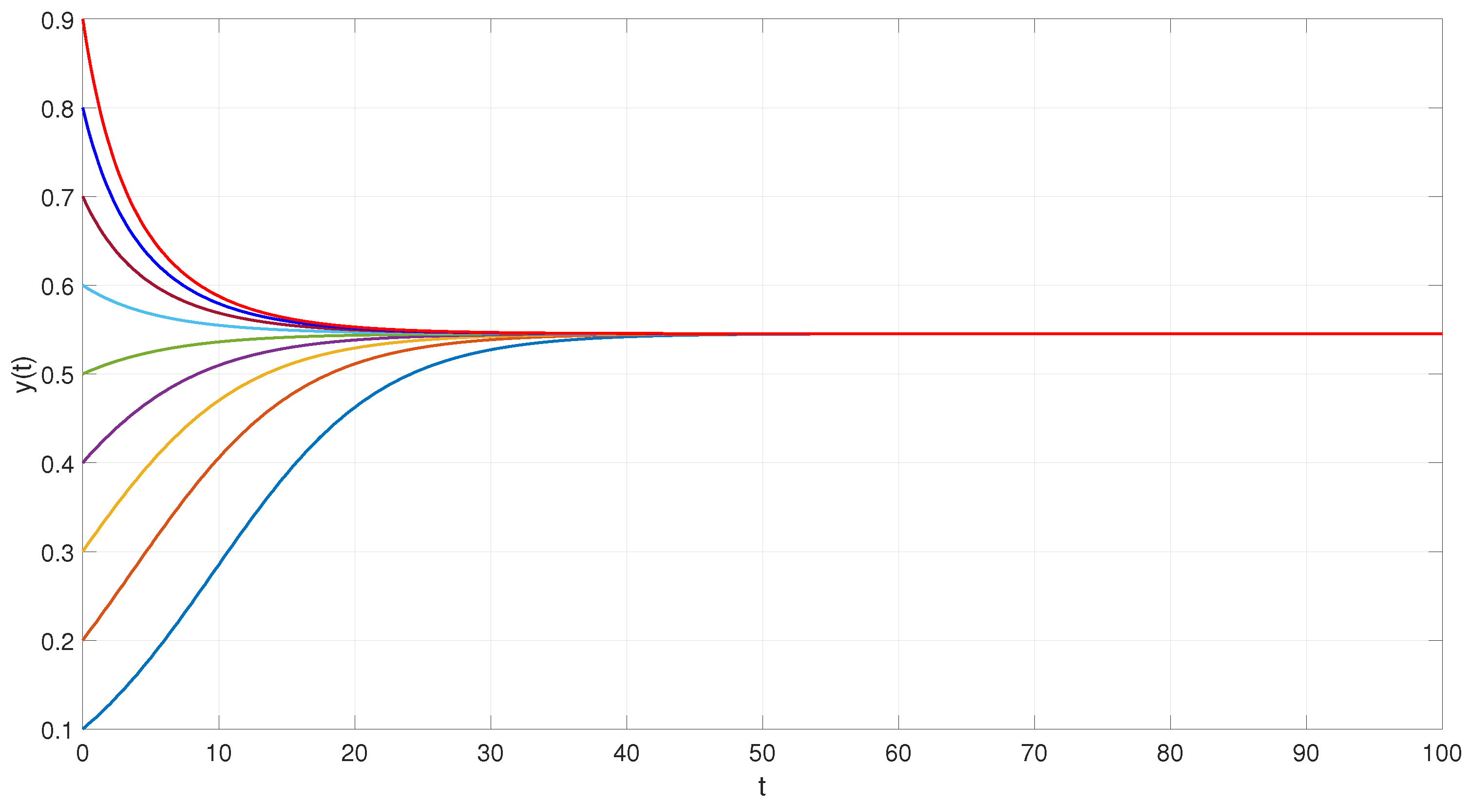
7. Examples and Simulations

In this section, two examples are presented to validate the theoretical results established in Theorems 3 and 4. Numerical simulations are conducted using MATLAB 2022, and the corresponding outcomes are illustrated in Figure 1 and Figure 2.

Example 1.

Consider the following epidemic model:

$$y^{\prime }\left(t\right)=0.15y\left(\left[t+0.5\right]\right)\left(1-y\left(t\right)\right)-0.23y\left(t\right),$$

(31)

where, $t\in {\mathbb{R}}^{+}$ and $[·]$ signifies the greatest integer function.

This model represents a particular case of the epidemic system with DEPCAG (2), where the parameters are given by $b=0.15$, $c=0.23$, $t_0={\gamma }_0=0$, $t_m=m-0.5$, ${\gamma }_m=m$ for $m\in \mathbb{N}$, and $\theta ={\theta }_m^{+}={\theta }_m^{-}=0.5$.

By straightforward computation, we find

$$\theta =0.5,0.15=b<c=0.23,$$

$$(2b+c)\theta =\rho =0.265<1,\mu =\left(b+(b+c)e^{\left(b+c+{\displaystyle \frac{b}{1-\rho }}\right)\theta }\right)\theta \approx 0.3294<1,$$

$${\displaystyle \frac{b}{1-\mu }}\approx 0.2237\le 0.23=c.$$

Hence, all the conditions stated in Theorem 3, namely (14), (19), and ${\displaystyle \frac{b}{1-\mu }}\le c$, are satisfied for the epidemic model (31). This ensures that the trivial equilibrium of the system is uniformly asymptotically stable within the invariant region $\Omega$.

To illustrate this result, we perform numerical simulations using MATLAB 2022. Figure 1 shows the trajectories of the system starting from randomly selected initial conditions. As depicted, all trajectories converge to a single uniformly stable equilibrium point.

Figure 1. Trajectories, represented by different colored lines, converging to the uniformly asymptotically stable equilibrium point of the epidemic model with DEPCAG (31).

Figure 1. Trajectories, represented by different colored lines, converging to the uniformly asymptotically stable equilibrium point of the epidemic model with DEPCAG (31).

This epidemic model, with infection rate $b=0.15$ and recovery rate $c=0.23$, reflects the average transmission intensity and the rate at which infected individuals recover or are removed from the infectious population per unit time, respectively.

In this case, the basic reproduction potential is sub-threshold, as $c>b$. The corresponding equilibrium is

$$y^{*}=1-{\displaystyle \frac{c}{b}}=1-{\displaystyle \frac{0.23}{0.15}}<0,$$

which is biologically infeasible, since it yields a negative value. Therefore, the only meaningful equilibrium is the disease-free state $y=0$. This implies that the infection cannot persist in the population and will eventually be eradicated, even in the presence of time delays introduced by the DEPCAG structure.

A key feature of this model is the incorporation of a deviated argument $y\left(\right[t+0.5\left]\right)$, where the square brackets denote a piecewise constant argument. Specifically, we define the partition points as $t_i=i-0.5$ and ${\gamma }_i=i$ for $i\in \mathbb{N}$, with the mapping $\gamma \left(t\right)={\gamma }_i$ on the interval $[t_i,t_{i+1})$. This construction divides each interval into two distinct subintervals:

• On $[t_i,{\gamma }_i]$, the model exhibits an advanced (anticipatory) structure, as ${\gamma }_i\ge t$. This segment captures the impact of forward-looking actions such as proactive isolation, anticipatory behavioral changes, or early government interventions based on projected epidemiological trends.
• On $({\gamma }_i,t_{i+1})$, the model reflects a retarded (delayed) response, where the effect of past states (e.g., incubation period, diagnosis delay) continues to impact current dynamics.

This alternation between advanced and retarded dynamics provides a flexible and realistic framework for modeling epidemic systems, accounting simultaneously for both preventive strategies and delayed biological or administrative effects. Notably, the anticipatory component $[t+0.5]$ plays a central role in representing predictive decision-making mechanisms that are increasingly relevant in modern public health responses.

Example 2.

Consider the following epidemic model:

$$y^{\prime }\left(t\right)=0.33y\left(\gamma \left(t\right)\right)\left(1-y\left(t\right)\right)-0.15y\left(t\right),$$

(32)

where $t\in {\mathbb{R}}^{+}$, $t_m=0.3m$, ${\gamma }_m=0.3m+0.3$, and $m\in \mathbb{N}$, with ${\theta }_m^{+}={\theta }_m^{-}=0.3$.

This example corresponds to a particular case of the epidemic model with DEPCAG (2), where the parameters are given by $b=0.33$ and $c=0.15$.

A straightforward computation yields

$$\theta =0.3,0.15=c<b=0.33,$$

$$(2b+c)\theta =\rho =0.243<1,\mu =\left(b+(b+c)e^{\left(b+c+{\displaystyle \frac{b}{1-\rho }}\right)\theta }\right)\theta \approx 0.2886<1,$$

$$\vartheta =c\left(1+{\displaystyle \frac{c}{b}}\right)\theta \approx 0.0655<1,\eta =c\left({\displaystyle \frac{c}{b}}+1\right)e^{c\left(1+{\displaystyle \frac{c}{b(1-\vartheta )}}\right)\theta }\theta \approx 0.0698,$$

$$\left(1+{\displaystyle \frac{1}{1-\eta }}\right)c\approx 0.3113\le 0.33=b.$$

We observe that all the conditions (14), (22), (26), and $\left(1+{\displaystyle \frac{1}{1-\eta }}\right)c\le b$ in Theorem 4 are satisfied for the epidemic model with DEPCAG (32). Therefore, the positive equilibrium of the model is uniformly stable.

Using MATLAB 2022, we performed simulations starting from random initial states. The results confirm the presence of a unique uniformly stable equilibrium point, as illustrated in Figure 2.

Figure 2. Trajectories, represented by different colored lines, converging to a uniformly stable equilibrium point of the epidemic model with DEPCAG (32).

Figure 2. Trajectories, represented by different colored lines, converging to a uniformly stable equilibrium point of the epidemic model with DEPCAG (32).

In this epidemic model, the infection rate $b=0.33$ and the recovery rate $c=0.15$ represent, respectively, the intensity of disease transmission and the speed of recovery or removal from the infectious class.

From these values, the model predicts a positive endemic equilibrium at

$$y^{*}=1-{\displaystyle \frac{c}{b}}=1-{\displaystyle \frac{0.11}{0.25}}=0.\overline{54}.$$

This implies that, in the absence of further interventions, the system tends toward a state where approximately 54% of the population remains infected in the long term. This equilibrium captures the balance between the infection pressure and the recovery dynamics.

8. Conclusions

This paper examines an epidemic model formulated using differential equations with piecewise constant arguments of the generalized type (DEPCAG). The significance of this model within the framework of population dynamics is evident. By incorporating a generalized piecewise constant argument, the model effectively captures the influence of past states on the present dynamics, underscoring the relevance of the results obtained. In real-world scenarios, historical conditions can profoundly impact current system behavior, often leading to substantial changes. Consequently, the selection of an appropriate argument in model construction is crucial. Furthermore, the incorporation of a future-dependent deviation argument introduces an anticipatory component, reflecting a qualitative prediction mechanism that integrates real-time decision-making. This anticipation may stem from complex factors beyond mere subjectivity. In this regard, the deviation argument considered in this study enhances the model’s applicability and contributes to its development. However, the presence of such an argument complicates the derivation of an explicit solution. Therefore, analyzing the system without explicitly solving it becomes a practical approach. To address this challenge, the study employs the Lyapunov–Razumikhin method, which facilitates stability analysis without requiring an exact solution. This approach provides computational advantages and methodological convenience compared to alternative techniques available in the literature, making it particularly suitable for examining epidemic models with DEPCAG.

Although this study focuses on rigorous theoretical analysis, future work will consider the implementation of numerical simulations to illustrate the dynamical behavior under realistic conditions. For example, epidemic scenarios with stepwise interventions such as lockdowns or testing regimes could be modeled using real-world data to estimate the parameters b, c, and $\gamma \left(t\right)$.

Potential extensions of this study include incorporating spatially heterogeneous diffusion terms to capture geographic spread or introducing stochastic perturbations to model uncertainty in infection dynamics, particularly relevant under fluctuating reporting practices or random environmental effects.

References

1. Cooke, K.L. Stability analysis for a vector disease model. Rocky Mt. J. Math. 1979, 7, 253–263. [Google Scholar] [CrossRef]
2. Huang, G.; Liu, A.; Fory’s, U. Global Stability analysis of some nonlinear delay differential equations in population dynamics. J. Nonlinear Sci. 2016, 26, 27–41. [Google Scholar] [CrossRef]
3. Busenberg, S.; Cooke, K.L. The effect of integral conditions in certain equations modelling epidemics and population growth. J. Math. Biol. 1980, 10, 13–32. [Google Scholar] [CrossRef] [PubMed]
4. Abta, A.; Boutayeb, S.; Laarabi, H.; Rachik, M.; Alaoui, H.T. Stability analysis of a delayed sir epidemic model with diffusion and saturated incidence rate. SN Partial. Differ. Equ. Appl. 2020, 1, 13. [Google Scholar] [CrossRef]
5. Liu, M.; Rost, G.; Vas, G. SIS model on homogeneous networks with threshold type delayed contact reduction. Comput. Math. Appl. 2013, 66, 1534–1546. [Google Scholar] [CrossRef]
6. Ramesh, N.; Reddy, B.R. Stability and hopf bifurcation analysis of a SIS epidemic model with time delay. J. Comput. Anal. Appl. (JoCAAA) 2024, 33, 972–981. [Google Scholar]
7. Alaoui, A.L.; Ammi, M.R.S.; Tilioua, M.; Torres, D.F. Global stability of a diffusive SEIR epidemic model with distributed delay. In Mathematical Analysis of Infectious Diseases; Elsevier: Amsterdam, The Netherlands, 2022; pp. 191–209. [Google Scholar]
8. Agaba, G.O.; Kyrychko, Y.N.; Blyuss, K.B. Time-delayed SIS epidemic model with population awareness. Ecol. Complex. 2017, 31, 50–56. [Google Scholar] [CrossRef]
9. Ghosh, S.; Volpert, V.; Banerjee, M. An Epidemic Model with Time Delay Determined by the Disease Duration. Mathematics 2022, 10, 2561. [Google Scholar] [CrossRef]
10. Zhao, S.; Lin, Q.; Ran, J.; Musa, S.; Yang, G.; Wang, W.; Lou, Y.; Gao, D.; Yang, L.; He, D.; et al. Preliminary estimation of the basic reproduction number of novel coronavirus (2019-nCoV) in China, from 2019 to 2020: A data-driven analysis in the early phase of the outbreak. Int. J. Infect. Dis. 2020, 92, 214–217. [Google Scholar] [CrossRef]
11. Wang, L.; Ruan, S. Modeling nosocomial infections of methicillin-resistant staphylococcus aureus with environment contamination. Sci. Rep. 2017, 7, 580. [Google Scholar] [CrossRef]
12. Li, J.; Ma, Z. Global analysis of SIS epidemic models with variable total population size. Math. Comput. Model. 2004, 39, 1231–1242. [Google Scholar]
13. Xu, R.; Ma, Z. Global stability of a SIR epidemic model with nonlinear incidence rate and time delay. Nonlinear Anal. Real World Appl. 2009, 10, 3175–3189. [Google Scholar] [CrossRef]
14. Wang, W.; Cai, Y.; Wu, M.; Wang, K.; Li, Z. Complex dynamics of a reaction-diffusion epidemic model. Nonlinear Anal. Real World Appl. 2012, 13, 2240–2258. [Google Scholar] [CrossRef]
15. Yang, J.; Liang, S.; Zhang, Y. Travelling waves of a delayed SIR epidemic model with nonlinear incidence rate and spatial diffusion. PLoS ONE 2011, 6, e21128. [Google Scholar] [CrossRef] [PubMed]
16. Xu, Z.; Chen, D. An SIS epidemic model with diffusion. Appl. Math. J. Chin. Univ. 2017, 32, 127–146. [Google Scholar] [CrossRef]
17. Pao, C.V. Dynamics of nonlinear parabolic systems with time delays. J. Math. Anal. Appl. 1996, 198, 751–779. [Google Scholar] [CrossRef]
18. Pao, C.V. Convergence of solutions of reaction–diffusion systems with time delays. Nonlinear Anal. Theory Methods Appl. 2002, 48, 349–362. [Google Scholar] [CrossRef]
19. Akhmet, M. Nonlinear Hybrid Continuous/Discrete-Time Models; Atlantis Press: Paris, France, 2011. [Google Scholar]
20. Chiu, K.-S. Periodic solutions for nonlinear integro-differential systems with piecewise constant argument. Sci. World J. 2014, 2014, 514854. [Google Scholar] [CrossRef]
21. Chiu, K.-S. Green’s function for periodic solutions in alternately advanced and delayed differential systems. Acta Math. Appl. Sin. Engl. Ser. 2020, 36, 936–951. [Google Scholar] [CrossRef]
22. Chiu, K.-S. Green’s function for impulsive periodic solutions in alternately advanced and delayed differential systems and applications. Commun. Fac. Sci. Univ. Ank. Ser. A1 Math. Stat. 2021, 70, 15–37. [Google Scholar] [CrossRef]
23. Chiu, K.-S. Periodicity and stability analysis of impulsive neural network models with generalized piecewise constant delays. Discret. Contin. Dyn. Syst. Ser. B 2021, 27, 659–689. [Google Scholar] [CrossRef]
24. Chiu, K.-S. Stability analysis of periodic solutions in alternately advanced and retarded neural network models with impulses. Taiwan. J. Math. 2022, 26, 137–176. [Google Scholar] [CrossRef]
25. Chiu, K.-S.; Berna, I. Nonautonomous impulsive differential equations of alternately advanced and retarded type. Filomat 2023, 37, 7813–7829. [Google Scholar] [CrossRef]
26. Dai, L. Nonlinear Dynamics of Piecewise Constant Systems and Implementation of Piecewise Constant Arguments; World Scientific: Singapore, 2008. [Google Scholar]
27. Huang, Z.; Wang, X.; Gao, F. The existence and global attractivity of almost periodic sequence solution of discrete-time neural networks. Phys. Lett. A 2006, 350, 182–191. [Google Scholar] [CrossRef]
28. Huang, Z.; Mohamad, S.; Xia, Y. Exponential periodic attractor of discrete-time BAM neural networks with transmission delays. Comput. Math. Model. 2009, 20, 258–277. [Google Scholar] [CrossRef]
29. Busenberg, S.; Cooke, K. Models of vertically transmitted diseases with sequential-continuous dynamics. In Nonlinear Phenomena in Mathematical Sciences; Lakshmikantham, V., Ed.; Academic Press: New York, NY, USA, 1982; pp. 179–187. [Google Scholar]
30. Chiu, K.-S. Periodic solutions of impulsive differential equations with piecewise alternately advanced and retarded argument of generalized type. Rocky Mt. J. Math. 2022, 52, 87–103. [Google Scholar] [CrossRef]
31. Chiu, K.-S. Existence and global exponential stability of periodic solution for Cohen-Grossberg neural networks model with piecewise constant argument. Hacet. J. Math. Stat. 2022, 51, 1219–1236. [Google Scholar] [CrossRef]
32. Chiu, K.-S. Almost periodic solutions of differential equations with generalized piecewise constant delay. Mathematics 2024, 12, 3528. [Google Scholar] [CrossRef]
33. Pinto, M. Asymptotic equivalence of nonlinear and quasi linear differential equations with piecewise constant arguments. Math. Comput. Model. 2009, 49, 1750–1758. [Google Scholar] [CrossRef]
34. Pinto, M. Cauchy and Green matrices type and stability in alternately advanced and delayed differential systems. J. Differ. Equ. Appl. 2011, 17, 235–254. [Google Scholar] [CrossRef]
35. Chiu, K.-S.; Córdova-Lepe, F. Global exponential periodicity and stability of neural network models with generalized piecewise constant delay. Math. Slovaca 2021, 71, 491–512. [Google Scholar] [CrossRef]
36. Balzotti, C.; D’Ovidio, M.; Loreti, P. Fractional SIS epidemic models. Fractal Fract. 2020, 4, 44. [Google Scholar] [CrossRef]
37. Wu, Z.; Cai, Y.; Wang, Z.; Wang, W. Global stability of a fractional order SIS epidemic model. J. Differ. Equ. 2023, 352, 221–248. [Google Scholar] [CrossRef]
38. Gray, A.; Greenhalgh, D.; Hu, L.; Mao, X.; Pan, J. A stochastic differential equation SIS epidemic model. SIAM J. Appl. Math. 2011, 71, 876–902. [Google Scholar] [CrossRef]
39. Hieu, N.; Nguyen, D.; Nguyen, N.; Tuong, T. Hybrid stochastic SIS epidemic models with vaccination: Stability of the disease-free state and applications. Nonlinear Anal. Hybrid Syst. 2024, 53, 101492. [Google Scholar] [CrossRef]
40. Sun, M.; Liu, Q. An SIS epidemic model with time delay and stochastic perturbation on heterogeneous networks. Math. Biosci. Eng. 2021, 18, 6790–6805. [Google Scholar] [CrossRef]
41. Guglielmi, N.; Iacomini, E.; Viguerie, A. Delay differential equations for the spatially resolved simulation of epidemics with specific application to COVID-19. Math. Methods Appl. Sci. 2022, 45, 4752–4771. [Google Scholar] [CrossRef]
42. Meziane, M.; Moussaoui, A.; Volpert, V. On a two-strain epidemic model involving delay equations. Math. Biosci. Eng. 2023, 20, 20683–20711. [Google Scholar] [CrossRef]
43. Achterberg, M.A.; Sensi, M. A minimal model for adaptive SIS epidemics. Nonlinear Dyn. 2023, 111, 12657–12670. [Google Scholar] [CrossRef]
44. Yang, P.; Jia, J.; Shi, W.; Feng, J.; Fu, X. Stability analysis and optimal control in an epidemic model on directed complex networks with nonlinear incidence. Commun. Nonlinear Sci. Numer. 2023, 121, 107206. [Google Scholar] [CrossRef]
45. Zerenner, T.; Lauro, F.D.; Dashti, M.; Berthouze, L.; Kiss, I.Z. Probabilistic predictions of SIS epidemics on networks based on population-level observations. Math. Biosci. 2022, 350, 108854. [Google Scholar] [CrossRef] [PubMed]
46. Zhou, Y.; Li, Y.; Zhang, Y. Numerical sensitivity analysis of the susceptible-infected-susceptible model on two-layer interconnected networks. Sci. Rep. 2025, 15, 9723. [Google Scholar] [CrossRef]
47. Li, Y.; Ruan, S.; Wang, Z. Asymptotic behavior of endemic equilibria for a SIS epidemic model in convective environments. J. Differ. Equ. 2025, 426, 606–659. [Google Scholar] [CrossRef]
48. Li, S.; Fu, T.; Yuan, R.; Sun, Y.; Liu, M. Dimensional reduction of an SIS epidemic network model with saturated treatment and human mobility. AIP Adv. 2025, 15, 045215. [Google Scholar] [CrossRef]
49. Wang, J.; Wang, K.; Zheng, T.; Zhou, P.; Teng, Z. Qualitative analysis on a reaction-diffusion SIS epidemic model with nonlinear incidence and Dirichlet boundary. Chaos Solitons Fractals 2024, 182, 114744. [Google Scholar] [CrossRef]
50. Yan, J.; Wang, H.; Li, X.; Tan, Y.g.; Ma, Y.; Zeng, M. A control measure for epidemic spread based on the susceptible–infectious–susceptible (SIS) model. Biosystems 2024, 246, 105341. [Google Scholar]
51. Peng, R.; Salako, R.; Wu, Y. Long-time dynamics of a parabolic-ODE SIS epidemic model with saturated incidence mechanism. Phys. Nonlinear Phenom. 2025, 481, 134747. [Google Scholar] [CrossRef]
Disclaimer/Publisher’s Note: The statements, opinions and data contained in all publications are solely those of the individual author(s) and contributor(s) and not of MDPI and/or the editor(s). MDPI and/or the editor(s) disclaim responsibility for any injury to people or property resulting from any ideas, methods, instructions or products referred to in the content.