Abstract
This study applies the Conformable Laplace Adomian Decomposition Method (CLADM) to solve generalized time-fractional Korteweg–de Vries (KdV) models, including seventh- and fifth-order models. CLADM combines the conformable fractional derivative and Laplace transform with the Adomian decomposition technique, offering analytic approximate solutions. Numerical and graphical results, generated using MATLAB R2020a 9.8.0.1323502, validate the method’s efficiency and precision in capturing fractional-order dynamics. Fractional parameters significantly influence wave behavior, with higher orders yielding smoother profiles and reduced oscillations. Comparative analysis confirms CLADM’s superiority over existing methods in minimizing errors. The versatility of CLADM highlights its potential for studying nonlinear wave phenomena in diverse applications.
Keywords:
nonlinear wave dynamics; time-fractional higher order KdV equations; conformable laplace adomian decomposition method MSC:
35R11; 35Q53
1. Introduction
The Korteweg–de Vries (KdV) model is a fundamental nonlinear partial differential equation that arises in the study of shallow water waves, plasma physics, and other physical systems. The KdV model is vital in understanding nonlinear wave dynamics across diverse physical phenomena, including flood analysis, plasma waves, and ocean surface waves. In ocean engineering, they are crucial for predicting tsunami wave evolution, understanding internal waves in stratified fluids, and analyzing rogue waves, all of which are essential for ensuring the stability of offshore structures and coastal protection. Furthermore, these models are particularly valuable for studying coastal wave dynamics and interactions between offshore structures and waves, offering critical insights for designing resilient coastal and marine infrastructure. Beyond fluid dynamics, the KdV model has significantly influenced several scientific domains, such as optics, quantum field theory, general relativity, plasma physics, and fluid mechanics. The origins of solitary wave research trace back to Russell’s discovery in 1834, during their observations of water waves while working on canal boat designs. Subsequent investigations by Boussinesq and Rayleigh in the 1870s provided critical insights that eventually led to the formulation of the classical KdV model by Korteweg and de Vries in 1895. Since then, various extensions and adaptations of the KdV model have emerged, including the modified KdV (mKdV), fifth-order KdV, generalized KdV and Hirota–Satsuma KdV equations. These variations have been introduced to address complex physical scenarios and enhance the applicability of the original model [1].
The seventh-order KdV model extends the classical KdV framework by incorporating higher-order dispersion and nonlinearity terms, enabling the modeling of more intricate wave phenomena. Researchers have applied the Adomian Decomposition Method (ADM) to approximate solutions of seventh-order KdV equations, enhancing the analytical tools available for complex nonlinear differential Equations [2]. The Homotopy Analysis Method (HAM) has also been utilized to derive approximate solutions, demonstrating the equation’s role in advancing analytical techniques for higher-order nonlinear problems [3]. The seventh-order KdV model has been analyzed to identify conservation laws, which are crucial for understanding the invariants and symmetries of complex nonlinear systems [4]. Studies have explored generalized solitary wave solutions within the framework of higher-order KdV models, including the seventh-order variant. These investigations contribute to the broader understanding of solitary wave behavior in nonlinear systems [5]. Ozkan derived exact solutions for the time-fractional seventh-order Sawada–Kotera–Ito model using the exp-function, (G′/G)-expansion, and ansatz methods, yielding dark, bright, and singular soliton solutions [6]. Mancas and Hereman investigated traveling-wave solutions to fifth- and seventh-order KdV models using elliptic function methods. Their research offers exact solutions that serve as benchmarks for numerical solvers and aid in understanding the dynamics of nonlinear wave models [7]. Research has been conducted on a seventh-order generalized KdV model and its fractional version in fluid mechanics using symmetry analysis. This work aids in understanding the role of symmetries in the solutions and conservation laws of higher-order KdV models [8].
The LADM has been employed to obtain numerical and approximate solutions for certain fifth-order KdV equations. This method integrates Laplace transforms with Adomian polynomials to efficiently manage nonlinear terms [9]. Studies have explored new closed-form solutions of the time-fractional fifth-order KdV model using Lie group analysis and the G′/G-expansion method, providing insights into the behavior of fractional-order nonlinear systems [10]. The trial equation method has been utilized to the fifth-order KdV equation to find exact solutions, aiding in the analysis of complex dynamic behaviors in fractional calculus [11]. The extended complex method has been utilized to explore exact solutions for the generalized fifth-order KdV model, providing insights into the equation’s integrability and solution structures [12]. The authors investigated the nonlinear variable-order fractional KdV equation, which models shallow water waves. They employed the modified (G′/G)-expansion method to derive exact solitary wave solutions and traveling wave solutions. The study contributes to the understanding of wave dynamics in shallow water by providing analytical solutions to this fractional differential Equation [13]. The authors investigated the generalized fifth-order KdV model, with fifth-order linear dispersion and cubic nonlinearity terms. They employed the modified exp-function method to derive exact traveling wave solutions, including solitary wave solutions. The study contributes to the understanding of wave dynamics in shallow water by providing analytical solutions to this nonlinear partial differential Equation [14]. The study explores the Kaup–Kupershmidt (KK) model, a particular variant of the fifth-order KdV model. The authors formulated the equation using a Lagrangian framework, derived associated conservation laws, and determined exact analytical solutions for ocean gravity waves described by this equation. This research provides valuable insights into the dynamics of waves in shallow water by presenting both analytical solutions and conservation principles for the KK model [15]. The authors proposed a robust fuzzy double parametric approach, specifically the q-Homotopy Analysis Shehu Transform Method (q-HAShTM), to solve the generalized fuzzy fractional KdV equation. This method incorporates Hukuhara differentiability and Shehu transform to handle uncertainties in the velocity profiles at various spatial positions [16].
Fractional KdV equations have been widely studied due to their significance in modeling nonlinear wave dynamics in various physical systems, including shallow water waves, ion-acoustic waves in plasma, and optical solitons. Researchers have applied various analytical and numerical techniques to study different forms of fractional KdV equations. Kurulay and Bayram employed the Differential Transform Method (DTM) to obtain approximate analytical solutions for the fractional modified KdV (fmKdV) and fractional KdV (fKdV) equations based on the Caputo fractional derivative [17]. Wang applied Lie symmetry analysis to the time-fractional fifth-order KdV equation, transforming it into an ordinary differential equation involving the Erdelyi–Kober fractional derivative [18]. Nazari-Golshan investigated the Space-Fractional Modified KdV (SFMKdV) equation using the Modified G′/G-expansion method, showing how space-fractional parameters influence ion acoustic wave propagation [19]. Alshammari investigated a fractional-order system of KdV equations using the Modified Decomposition Method (MDM) and the New Iterative Transform Method (NITM), demonstrating their effectiveness in obtaining accurate analytical approximations while reducing computational costs [20]. Cao developed efficient finite difference schemes for solving the time-fractional KdV equation, proving their unique solvability, boundedness, and high convergence order [21]. Yousif applied a conformable-Caputo fractional nonpolynomial spline method, enhancing computational efficiency for solving fractional KdV Equations [22]. Dwivedi and Sarkar developed a Crank–Nicolson Fourier-spectral-Galerkin scheme, ensuring the preservation of integral invariants in long-term simulations of fractional KdV-type models [23]. Gu introduced a local discontinuous Galerkin method with generalized alternating numerical fluxes, improving numerical accuracy in fractional KdV models [24].
Moreover, while several studies have used fractional derivatives such as Caputo, Riemann–Liouville, and Erdelyi–Kober, the use of conformable fractional derivatives remains an area of active research due to their computational simplicity and ability to approximate fractional-order behavior effectively. Khalil [25] introduced the conformable fractional derivative (CFD), a modern extension of the traditional limit-based definition of a derivative. Owing to its simplicity, this derivative has been extensively applied in conjunction with various methods [26,27,28,29] across numerous contexts. This study employs the Conformable Laplace Adomian Decomposition Method (CLADM) to solve generalized time-fractional KdV models, focusing on seventh- and fifth-order models. Specifically, we examine the fifth-order time-fractional KdV Sawada–Kotera (SK) model, the time-fractional seventh-order KdV Sawada–Kotera–Ito (SKI) model, Kaup–Kuperschmidt (KK) model, and Lax model. These models are highly significant for modeling nonlinear wave phenomena, particularly in oceanography and ocean engineering, where they describe the propagation of shallow water waves, solitons, and other dispersive wave behaviors. The fractional-order derivatives in these equations provide a more accurate representation of complex physical processes, such as wave dispersion and dissipation, which are vital for understanding ocean dynamics and mitigating risks in coastal engineering projects. To validate our approach, we compare the CLADM solutions with exact solutions both numerically and graphically, demonstrating the method’s accuracy and efficiency. The CLADM is chosen for its ability to handle nonlinear fractional differential equations effectively, offering advantages such as reduced computational complexity, high precision in approximating solutions, and the ability to provide analytical solutions in series form. This makes CLADM particularly well-suited for solving complex fractional-order models like the ones studied here. Our work not only advances the theoretical understanding of these models but also provides practical tools for analyzing real-world phenomena in oceanography and ocean engineering.
2. Concept of CLADM for FPDEs
Definition 1
(see [25]). Given a function , then the Conformable Fractional Derivative of order ϱ is given by
for all
Definition 2
(see [30]). Let Ω is an n times differentiable at τ. Then, the conformable fractional derivative of Ω of order ϱ is defined as:
for all and is the smallest integer greater than or equal to ϱ.
Let us next investigate the basic fractional Laplace transform [30].
Definition 3
(see [30,31]). Let and be real valued function. Then, the Laplace transform for fractional order ϱ is defined by:
where .
The Laplace transform in the conformable fractional-order sense is described as
The usual and fractional Laplace transform has the following relation.
Theorem 1
(see [31]). Let be a function, and if exists, then
where .
Theorem 2
(see [32,33]). If is a given series;
- 1.
- If such that , then the given series solution is convergent.
- 2.
- If such that , then the given series solution is divergent.
Consider the following FPDEs forms:
where .
The fractional derivative in Equation (4) is considered in the conformable sense in , is the highest-order classical derivative operator in , is other lower-order derivative terms, is the nonlinear term, and is the sources term with the initial condition.
Applying the conformable Laplace transform with respect to both sides of Equation (4), we have
By applying property Equation (2) of conformable Laplace transform, Equation (6) becomes
Which can be written as,
In Equation (8), applying inverse Laplace transform in conformable sense, we have
where the nonlinear term of Equation (4) is handled by applying ADM and the solution is expressed as an infinite sum of series:
where Adomian polynomials are given by,
By substituting Equations (10) and (11) into Equation (9),
When comparing both sides of Equation (13), we get the following recursive relation:
In general, the relation can be written as
where
The solution can be obtained from Equation (10).
3. Application of CLADM on KdV Time-Fractional Models
This study extends the CLADM to solve fifth-order time-fractional KdV models, specifically the SK model. This model can be expressed in the form of the generalized fifth-order time-fractional KdV equation:
where and ’s are arbitrary and nonzero parameters. The well-known Sawada–Kotera model is obtained by setting , , and in Equation (18) [34,35].
A general form of time-fractional seventh-order KdV model is written by [1]:
where and s are arbitrary and nonzero parameters.
Example 1.
Consider the time fractional fifth-order KdV SK model:
where and subject to the initial condition
Solution: By applying CLADM on Equation (20) discussed in Section 2, we can have
From the initial condition Equation (21), we get
The solution of Equation (20) is obtained in the form of Equation (10).
The exact solution of Equation (20) is given by:
Example 2.
Consider the time fractional seventh-order KdV KK model (by setting , , , , , , in Equation (19)):
where and with initial condition
Solution: By applying CLADM on Equation (28) discussed in Section 2, we will have
From the initial condition Equation (29), we get
The solution of Equation (28) is obtained in the form of Equation (10).
The exact solution of Equation (28) is given by:
Example 3.
Consider the time fractional seventh-order KdV SKI model (by setting , , , , , , in Equation (19)):
where and with the initial condition
Solution: By applying CLADM on Equation (36) discussed in Section 2, we will have
From the initial condition Equation (37), we get
The solution of Equation (36) is obtained in the form of Equation (10).
The exact solution of Equation (36) is given by:
Example 4.
Consider the time fractional seventh-order KdV Lax model (by setting , , , , , , in Equation (19)):
where and with the initial condition
Solution: By applying CLADM on Equation (44) discussed in Section 2, we will have
From the initial condition Equation (45), we get
The solution of Equation (44) is obtained in the form of Equation (10).
The exact solution of Equation (44) is given by:
4. Result and Discussion
This research investigates a fifth-order and a general seventh-order time-fractional KdV model solved through the Laplace Adobian Decomposition Method (LADM) in a conformable sense. By adjusting the parameters ’s in the seventh-order KdV model, the study examines specific cases of the time-fractional SKI, KK, and Lax KdV models. The primary objective is to explore their fractional nature, emphasizing dynamic properties and the computational efficiency of the CLADM.
In addition to the analysis of convergence of the series solution, we calculated the terms using Theorem 2.
For the fifth-order KdV model solution, we obtained, , , .
Similarly, for the seventh-order KdV KK model solution, we have, , , .
Also, for seventh-order KdV SKI model solution, we have, , , .
For the seventh-order KdV Lax model solution, we have, , , .
Hence, all the obtained series solutions are convergent.
The results for the time-fractional fifth-order KdV model (Example 1) underscore the adaptability of the CLADM Method. Table 1 illustrates the comparative analysis of solutions by the CLADM and exact. Numerical comparison of absolute errors Table 2 demonstrate that the CLADM achieves superior accuracy compared to conventional methods such as the HAM, particularly for higher fractional orders. Figure 1 superposes the surface produced by the proposed CLADM scheme on the exact fractional KdV solution. The two surfaces coincide so closely that they are visually indistinguishable at the plot’s resolution, with the highest wave amplitude at the origin gradually tapering off with increasing spatial distance. The fractional parameter significantly influences wave steepness and amplitude; as approaches unity, the wave profiles become smoother, aligning with classical dynamics.

Table 1.
CLADM numerical comparison of , with a KdV fifth-order fractional model, with .
Table 2.
CLADM numerical comparison of , with a KdV fifth-order fractional model, at and .
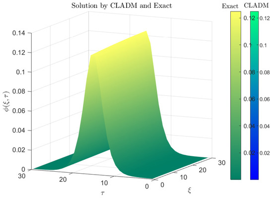
Figure 1.
Solution graph of time-fractional fifth-order KdV model by CLADM and Exact.
A 2D diagram, as shown in Figure 2a,b, showcasing the wave surface levels at various values highlights the gradual flattening of waves as fractional effects diminish. Figure 3 illustrates the absolute error distribution of the numerical solution for the fifth-order KdV equation over the spatial domain and temporal interval with parameter . The graph demonstrates how the numerical approximation deviates from the exact solution. It can be seen that the error remains consistently low throughout the domain, with minor fluctuations over time and space.
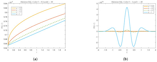
Figure 2.
Fifth-order KdV model when (a) and and (b) and .
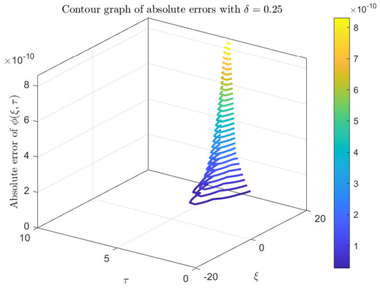
Figure 3.
Absolute error graph of time-fractional fifth-order KdV model with .
In the analysis of the KdV KK model (Example 2), absolute errors are calculated for various time and space parameters and are compared against results obtained using the exact solution. The comparative results Table 3 consistently highlight the precision of the CLADM, demonstrating significantly lower errors. Furthermore, as shown in Table 4, errors decrease with increasing fractional order, suggesting enhanced accuracy of wave propagation models in near-classical regimes. The graphical analysis offers additional insights into the wave behavior. For the Lax KdV model, a 3D visualization of approximate solutions and exact solution Figure 4 reveals that wave amplitude peaks at and diminishes with increasing distance. Fractional order plays a critical role in wave dynamics, as illustrated in Figure 5a, where higher values result in flatter wave profiles, indicating reduced steepness. Additionally, the 2D diagram in Figure 5b demonstrates that increasing leads to an enlargement in wave surface levels while dampening oscillations with distance from the origin. Figure 6 presents the absolute error profile for the numerical solution of the seventh-order KdV-KK equation over the spatial domain and time interval with parameter . From the figure, it is evident that the error remains extremely low throughout the entire domain. This demonstrates the high accuracy and numerical stability of the computational scheme.
Table 3.
CLADM numerical comparison of , with a KdV seventh-order KK fractional model, with .
Table 4.
CLADM numerical comparison of , with a KdV seventh-order KK fractional model, at and .
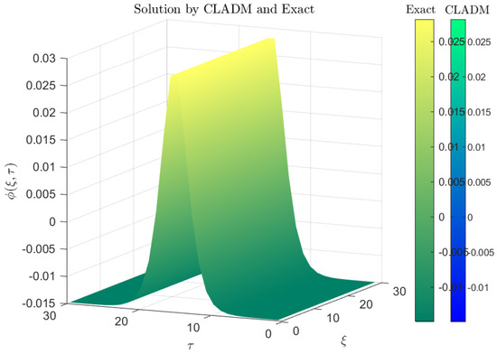
Figure 4.
Solution graph of time-fractional KdV seventh-order KK model by CLADM and Exact.
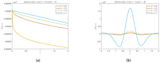
Figure 5.
KdV seventh-order KK model when (a) and and (b) and .
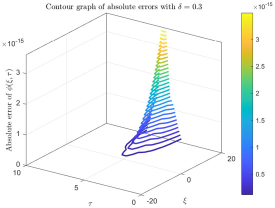
Figure 6.
Absolute error graph of time-fractional seventh-order KdV KK model with .
For the KdV SKI model (Example 3), a similar trend is observed. Numerical comparison of distinct fractional order and absolute error Table 5 and Table 6 validate the efficiency of the CLADM over HAM [3], with reduced error magnitudes as fractional order increases. The 3D solution Figure 7 further confirm the robustness of the CLADM. In Figure 8a, higher values correlate with increased wave amplitudes. Additionally, the 2D graphs in Figure 8b for fixed time periods highlight the same trends, underscoring the model’s fidelity in capturing intricate wave dynamics. Figure 9 presents the absolute error profile for the numerical solution of the seventh-order KdV-SKI equation over the spatial domain and time interval with parameter . Compared to other fifth- and seventh-order models, this result shows a relatively higher error, which can be attributed to the lower dispersion strength.
Table 5.
CLADM numerical comparison of , with a KdV seventh-order SKI fractional model, with .
Table 6.
CLADM numerical comparison of , with a KdV seventh-order SKI fractional model, at and .
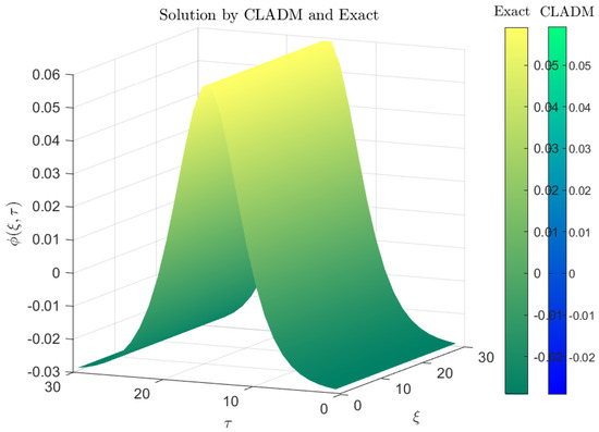
Figure 7.
Solution graph of time-fractional KdV seventh-order SKI model by CLADM and Exact.
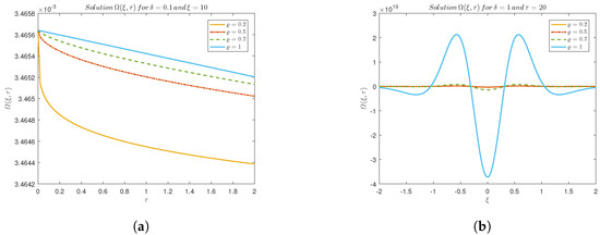
Figure 8.
KdV seventh-order SKI model when (a) and and (b) and .
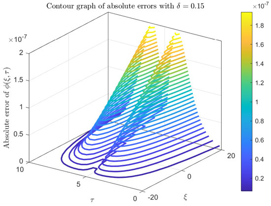
Figure 9.
Absolute error graph of time-fractional seventh-order KdV SKI model with .
In the KdV Lax model (Example 4), numerical comparison of absolute error Table 7 and Table 8 reinforce the reliability of the CLADM for complex fractional models. The 3D solution and error visualizations Figure 10 reflect the accuracy of the method, while Figure 11a,b illustrates how the water surface level increases with higher fractional parameters. Figure 12 presents the absolute error profile for the numerical solution of the seventh-order KdV-Lax equation over the spatial domain and time interval with parameter . From the figure, it is evident that the error remains extremely low throughout the entire domain.
Table 7.
CLADM numerical comparison of , with a KdV seventh-order Lax fractional model, with .
Table 8.
CLADM numerical comparison of , with a KdV seventh-order Lax fractional model, at and .
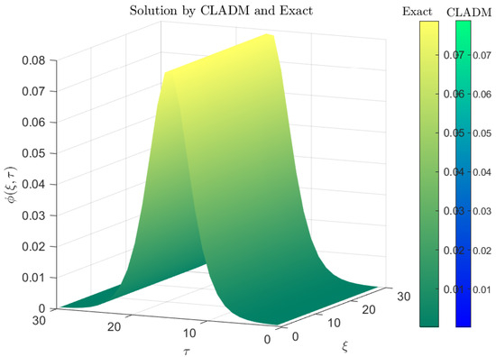
Figure 10.
Solution graph of time-fractional KdV seventh-order Lax model by CLADM and Exact.
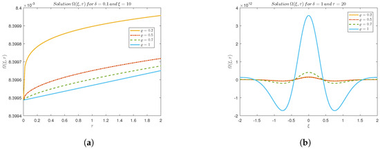
Figure 11.
KdV seventh-order Lax model when (a) and and (b) and .
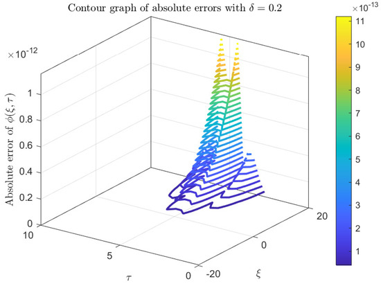
Figure 12.
Absolute error graph of time-fractional seventh-order KdV Lax model with .
5. Conclusions
This study demonstrates the effectiveness of the Conformable Laplace Adobian Decomposition Method (CLADM) in solving generalized time fractional seventh-order Sawada–Kotera–Ito, Kaup–Kuperschmidt, Lax, and the fifth-order KdV models. The results highlight the significant impact of fractional parameters on wave dynamics, with increasing yielding smoother wave profiles and reduced oscillations, aligning closely with classical integer-order behavior. Comparisons with existing methods, such as HAM and HLM, confirm CLADM’s superior accuracy in minimizing absolute errors. Graphical and numerical analyses validate its versatility in addressing complex fractional dynamics and initial conditions across different models. In conclusion, CLADM is a reliable and efficient approach for solving fractional-order nonlinear equations. It handles any problem whose fractional operator admits a Laplace image and whose nonlinearity is analytic. That spans single- and multi-term FODEs, time-fractional PDEs, coupled or delay systems, integro-differential forms, and even variable-order kernels. Its adaptability suggests strong potential for future research into multi-dimensional solitonic systems and other nonlinear wave phenomena.
Author Contributions
Methodology, P.V.T. and A.P.; Software, A.P.; Validation, P.V.T. and A.P.; Formal analysis, P.V.T. and T.P.; Investigation, A.P. and T.P.; Writing—original draft, A.P.; Writing—review & editing, T.P.; Supervision, P.V.T. All authors have read and agreed to the published version of the manuscript.
Funding
This research received no external funding.
Data Availability Statement
The original contributions presented in this study are included in the article. Further inquiries can be directed to the corresponding author.
Conflicts of Interest
There are no conflicts of interests regarding the publication of this manuscript.
References
- Qayyum, M.; Ahmad, E.; Saeed, S.T.; Akgul, A.; Riaz, M.B. Traveling wave solutions of generalized seventh-order time-fractional kdv models through he-laplace algorithm. Alex. Eng. J. 2023, 70, 1–11. [Google Scholar] [CrossRef]
- Alzaid, N.A.; Alrayiqi, B.A. Approximate solution method of the seventh order kdv equations by decomposition method. J. Appl. Math. Phys. 2019, 7, 2148–2155. [Google Scholar] [CrossRef][Green Version]
- Arora, R.; Sharma, H. Application of ham to seventh order kdv equations. Int. J. Syst. Assur. Eng. Manag. 2016, 9, 131–138. [Google Scholar] [CrossRef]
- Bruzon, M.; Marquez, A.; Garrido, T.; Recio, E.; de la Rosa, R. Conservation laws for a generalized seventh order kdv equation. J. Comput. Appl. Math. 2019, 354, 682–688. [Google Scholar] [CrossRef]
- Joshi, N.; Lustri, C.J. Generalized solitary waves in a finite-difference korteweg-de vries equation. Stud. Appl. Math. 2019, 142, 359–384. [Google Scholar] [CrossRef]
- Guner, O. New exact solutions for the seventh-order time fractional sawada–kotera–ito equation via various methods. Waves Random Complex Media 2018, 30, 441–457. [Google Scholar] [CrossRef]
- Mancas, S.C.; Hereman, W.A. Traveling wave solutions to fifth- and seventh-order korteweg–de vries equations: Sech and cn solutions. J. Phys. Soc. Jpn. 2018, 87, 114002. [Google Scholar] [CrossRef]
- Wang, G.; Liu, Y.; Wu, Y.; Su, X. Symmetry analysis for a seventh-order generalized kdv equation and its fractional version in fluid mechanics. Fractals 2020, 28, 2050044. [Google Scholar] [CrossRef]
- Handibag, S.; Karande, B.D. Existence the solutions of some fifth-order kdv equation by laplace decomposition method. Am. J. Comput. Math. 2013, 3, 80–85. [Google Scholar] [CrossRef][Green Version]
- Wang, Z.; Sun, L.; Hua, R.; Su, L.; Zhang, L. Time-fractional generalized fifth-order kdv equation: Lie symmetry analysis and conservation laws. Front. Phys. 2023, 11, 1133754. [Google Scholar] [CrossRef]
- Liu, T. Exact solutions to time-fractional fifth order kdv equation by trial equation method based on symmetry. Symmetry 2019, 11, 742. [Google Scholar] [CrossRef]
- Rehman, M.F.U.; Gu, Y.; Yuan, W. Exact analytical solutions of generalized fifth-order kdv equation by the extended com-plex method. J. Funct. Spaces 2021, 2021, 1–9. [Google Scholar] [CrossRef]
- Ali, U.; Ahmad, H.; Abu-Zinadah, H. Soliton solutions for nonlinear variable-order fractional korteweg–de vries (kdv) equation arising in shallow water waves. J. Ocean Eng. Sci. 2022, 9, 50–58. [Google Scholar] [CrossRef]
- Shakeel, A.M.; Alaoui, M.K.; Zidan, A.M.; Shah, N.A. Closed form solutions for the generalized fifth-order kdv equation by using the modified exp-function method. J. Ocean Eng. Sci. 2022. [Google Scholar] [CrossRef]
- Akbulut, A.; Kaplan, M.; Kaabar, M.K. New conservation laws and exact solutions of the special case of the fifth-order kdv equation. J. Ocean Eng. Sci. 2022, 7, 377–382. [Google Scholar] [CrossRef]
- Verma, L.; Meher, R.; Avazzadeh, Z.; Nikan, O. Solution for generalized fuzzy fractional kortewege-de varies equation us-ing a robust fuzzy double parametric approach. J. Ocean Eng. Sci. 2023, 8, 602–622. [Google Scholar] [CrossRef]
- Kurulay, M.; Bayram, M. Approximate analytical solution for the fractional modified kdv by differential transform method. Commun. Nonlinear Sci. Numer. Simul. 2010, 15, 1777–1782. [Google Scholar] [CrossRef]
- Wang, G.-W.; Liu, X.-Q.; Zhang, Y.-Y. Lie symmetry analysis to the time fractional generalized fifth-order kdv equation. Commun.—Tions Nonlinear Sci. Numer. Simul. 2013, 18, 2321–2326. [Google Scholar] [CrossRef]
- Nazari-Golshan, A. Derivation and solution of space fractional modified korteweg de vries equation. Commun. Nonlinear Sci. Numer. Simul. 2019, 79, 104904. [Google Scholar] [CrossRef]
- Alshammari, M.; Iqbal, N.; Mohammed, W.W.; Botmart, T. The solution of fractional-order system of kdv equations with exponential-decay kernel. Results Phys. 2022, 38, 105615. [Google Scholar] [CrossRef]
- Cao, H.; Cheng, X.; Zhang, Q. Numerical simulation methods and analysis for the dynamics of the time-fractional kdv equation. Phys. D Nonlinear Phenom. 2024, 460, 134050. [Google Scholar] [CrossRef]
- Yousif, M.A.; Hamasalh, F.K.; Zeeshan, A.; Abdelwahed, M. Efficient simulation of time-fractional korteweg-de vries equation via conformable-caputo non-polynomial spline method. PLoS ONE 2024, 19, e0303760. [Google Scholar] [CrossRef] [PubMed]
- Dwivedi, M.; Sarkar, T. Numerical method for the zero dispersion limit of the fractional korteweg-de vries equation. arXiv 2024. [Google Scholar] [CrossRef]
- Gu, Y. High-order numerical method for the fractional korteweg-de vries equation using the discontinuous galerkin method. AIMS Math. 2025, 10, 1367–1383. [Google Scholar] [CrossRef]
- Khalil, R.; Al Horani, M.; Yousef, A.; Sababheh, M. A new definition of fractional derivative. J. Comput. Appl. Math. 2014, 264, 65–70. [Google Scholar] [CrossRef]
- Ahmed, S.A. An efficient new technique for solving nonlinear problems involving the conformable fractional derivatives. J. Appl. Math. 2024, 2024, 5958560. [Google Scholar] [CrossRef]
- Hashemi, M. Invariant subspaces admitted by fractional differential equations with conformable derivatives. Chaos Solitons Fractals 2018, 107, 161–169. [Google Scholar] [CrossRef]
- Osman, W.M.; Elzaki, T.M.; Siddig, N.A. Modified double conformable laplace transform and singular fractional pseudo-hyperbolic and pseudo-parabolic equations. J. King Saud Univ.—Sci. 2021, 33, 101378. [Google Scholar] [CrossRef]
- Ayata, M.; Ozkan, O. A new application of conformable laplace decomposition method for fractional newell-whitehead-segel equation. AIMS Math. 2020, 5, 4702–4712. [Google Scholar] [CrossRef]
- Abdeljawad, T. On conformable fractional calculus. J. Comput. Appl. Math. 2015, 279, 57–66. [Google Scholar] [CrossRef]
- Silva, F.S.; Moreira, D.M.; Moret, M.A. Conformable laplace transform of fractional differential equations. Axioms 2018, 7, 55. [Google Scholar] [CrossRef]
- Maisuria, M.A.; Tandel, P.V. Mathematical modelling and application of reduced differential transform method for river pollution. Ratio Math. 2023, 47, 342–366. [Google Scholar] [CrossRef]
- More, P.A.; Tandel, P.V. Study of parametric effect on saturation rate in imbibition phenomenon for various porous materials. J. Ocean Eng. Sci. 2024, 9, 278–292. [Google Scholar] [CrossRef]
- Liu, C.; Dai, Z. Exact soliton solutions for the fifth-order sawada–kotera equation. Appl. Math. Comput. 2008, 206, 272–275. [Google Scholar] [CrossRef]
- Guo, Y.; Li, D.; Wang, J. The new exact solutions of the fifth-order sawada–kotera equation using three wave method. Appl. Math. Lett. 2019, 94, 232–237. [Google Scholar] [CrossRef]


Disclaimer/Publisher’s Note: The statements, opinions and data contained in all publications are solely those of the individual author(s) and contributor(s) and not of MDPI and/or the editor(s). MDPI and/or the editor(s) disclaim responsibility for any injury to people or property resulting from any ideas, methods, instructions or products referred to in the content. |
© 2025 by the authors. Licensee MDPI, Basel, Switzerland. This article is an open access article distributed under the terms and conditions of the Creative Commons Attribution (CC BY) license (https://creativecommons.org/licenses/by/4.0/).