Analyzing Competing Risks with Progressively Type-II Censored Data in Dagum Distributions

Abstract

Competing risk models are essential in survival analysis for studying systems with multiple mutually exclusive failure events. This study investigates the application of competing risk models in the presence of progressively Type-II censored data for the Dagum distribution, a flexible distribution suited for modeling data with heavy tails and varying skewness and kurtosis. The methodology includes maximum likelihood estimation of the unknown parameters, with a focus on the special case of a common shape parameter, which allows for a closed-form expression of the relative risks. A hypothesis test is developed to assess the validity of this assumption, and both asymptotic and bootstrap confidence intervals are constructed. The performance of the proposed methods is evaluated through Monte Carlo simulations, and their applicability is demonstrated with a real-world example.

1. Introduction

Competing risk models are valuable tools in survival analysis that address scenarios where individuals or systems face multiple mutually exclusive failure events. In such models, the event of interest is influenced by competing events that can prevent or modify the occurrence of the primary event. Competing risk models enable a more comprehensive understanding of the probabilities and cumulative incidences associated with different failure types. They provide insights into the relative risks and dynamics of competing events over time. These models have diverse applications across various fields, including healthcare, epidemiology, actuarial science, and engineering. By accounting for competing risks, researchers and practitioners can make informed decisions, develop appropriate risk management strategies, and gain a deeper understanding of complex systems’ failure patterns.

For example, in healthcare, competing risk models can be applied to study patient outcomes where different causes (e.g., death from different diseases) might prevent the observation of the event of primary interest, such as disease recurrence (see, e.g., [1]). In epidemiology, these models allow for the analysis of disease outcomes where various risks, like co-occurring conditions, compete (see, e.g., [2]). Actuarial science uses them to predict life insurance risks and policy lapses (see, e.g., [3]), while engineering applies them to assess system reliability where different failure modes compete for priority (see, e.g., [4]).

Censoring is a widely recognized and effective approach for cost reduction in experimental settings. In the field of reliability and survival analysis, numerous censoring strategies have been developed and employed by researchers. The two primary censoring plans, namely Type-I and Type-II, allow for the control of the overall duration of the experiment and the number of observed failures, respectively.

Progressive Type-II censoring is a censoring scheme that has gained considerable attention in the field of life testing and reliability analysis that was first introduced by [5,6]. It is designed to enhance the efficiency of experiments where the objective is to study the lifetimes or failure times of a set of items. In this censoring plan, a predetermined number of failures, denoted as m, is specified before the experiment begins. The censoring scheme, represented by $R=(R_1,R_2,\dots ,R_m)$, is carefully devised such that the sum of the individual censoring values, $R_1+R_2+\dots +R_m$, equals the difference between the total number of items, n, and the specified number of failures, m, i.e., $n-m$. Throughout the course of the experiment, items are progressively removed in stages, starting with the elimination of $R_1$ items after the first failure occurs. This sequential removal process continues until the mth failure, where the remaining $R_m$ items are also removed from the experiment. The progressive Type-II censoring scheme holds promise for optimizing the efficiency of experimental designs and has been extensively explored by researchers aiming to extract meaningful insights from reliability and survival analysis. For an excellent overview and in-depth discussions on progressive censoring, interested readers are encouraged to refer to the monograph authored by [7] (see also [8,9]).

Several authors have studied the competing risk models for common lifetime distributions based on progressive Type-II censored data. Ref. [10] studied the exponential model. Refs. [11,12] considered the Weibull model. Refs. [13,14,15,16] focused on the competing risk data for the Lomax, Kumaraswamy, Burr Type-XII and generalized Rayleigh distributions.

Ref. [17] analyzed the two-parameter Log-Normal model for hybrid Type-II progressive censored data. Ref. [18] introduced a competing risk exponential model utilizing a generalized Type I hybrid censoring method. The generalized exponential and the Weibull competing risk models under adaptive Type-II progressive censored data were studied, respectively, by [16,19]. Ref. [20] studied the statistical inference for a class of exponential distributions with Type-I progressively interval-censored competing risk data. Ref. [21] considered generalized progressive hybrid censoring for Burr XII competing distributions.

Bayesian inference for competing risk models has been explored by [12,22] for the Weibull model, and by [23] for the Gompertz model (see also [24,25,26,27], among others).

The case of dependent competing risks was studied by [28] for Marshall–Olkin bivariate Kumaraswamy distribution, and [29] for the Burr-XII model (see also [30] among others).

The Dagum distribution, alternatively referred to as Burr Type-III, was initially introduced by [31] as the third solution to the Burr differential equation, which characterizes the various types of Burr distributions. The Dagum distribution, introduced by [32], is widely applied in diverse fields such as finance, economics, and hydrology. It is characterized by its flexibility in modeling a wide range of data, particularly those with heavy tails and skewness. The Dagum distribution offers a flexible framework for analyzing data with varying shapes and tail behaviors, making it a valuable tool for researchers and practitioners seeking to understand and model complex phenomena.

The probability density function (pdf) of the two-parameter Dagum distribution, denoted as $D(\alpha ,\beta )$, is given by the following expression:

$$f(\alpha ,\beta ;x)=\alpha \beta x^{-(\beta +1)}{(1+x^{-\beta })}^{-(\alpha +1)},x>0$$

where $\alpha >0$ and $\beta >0$ are both shape parameters. The cumulative distribution function can be expressed in a simple form as follows:

$$F(\alpha ,\beta ;x)={(1+x^{-\beta })}^{-\alpha }.$$

The Dagum distribution is commonly referred to as the inverse Burr distribution. This connection arises from the fact that if a random variable X follows the Dagum distribution, its reciprocal ${\displaystyle \frac{1}{X}}$ follows the Burr Type-XII distribution, or simply the Burr distribution. For a comprehensive examination of the Dagum distribution, interested readers are encouraged to refer to the extensive study conducted by [33].

Despite the extensive literature on competing risk models under common lifetime distributions, such as exponential and Weibull, there is limited research on the application of the Dagum distribution with progressively Type-II censored data. This work addresses this gap by developing an inferential framework for the Dagum distribution under competing risks and various censoring schemes. Additionally, distributions with finite support such as Kies-style models (see [34]) could be explored as alternatives to the Dagum model for bounded failure times (see also [35]).

Moreover, while several heavy-tailed distributions (e.g. Pareto, Weibull, log-normal) have been employed in reliability analysis, the Dagum distribution offers unique advantages that make it especially attractive for modeling component lifetimes under complex censoring schemes. First, unlike the one-parameter Pareto model, whose mean is infinite when the shape parameter does not exceed unity, the Dagum distribution admits finite moments even in pronounced heavy-tail regimes, ensuring well-defined reliability measures [36]. Second, whereas the Weibull distribution enforces a monotonic hazard and the log-normal produces a strictly increasing-then-decreasing failure rate, the Dagum’s hazard function can assume bathtub, unimodal, or monotonic shapes, thereby capturing a wider range of empirical failure-mechanism behaviors observed in engineering applications [37]. Third, all key functions of the Dagum model (PDF, CDF, and hazard) have closed-form expressions, which greatly facilitates both classical and Bayesian inference under various types of censoring schemes. These combined features, flexible tail behavior, versatile hazard shapes, and analytic tractability underscore the Dagum distribution’s suitability for competing risks systems, as explored in the present work.

This paper is structured as follows. Section 2 introduces the competing risk models and their structure for the Dagum distribution. Section 3 discusses the maximum likelihood estimation of the unknown Dagum parameters, considering both the general case of arbitrary distribution parameters and the special case of a common shape parameter, $\beta$. Additionally, a likelihood ratio test procedure for testing the validity of the common shape parameter $\beta$ is presented. Section 4 is devoted to the asymptotic confidence intervals based on the Fisher information matrix, along with bootstrap confidence intervals. In Section 5, we evaluate the performance of our inference procedure through extensive Monte Carlo simulations. Finally, we illustrate the proposed methods with a real data example in Section 6.

2. Competing Risk Model Description

Suppose there are n units involved in an experiment, and there are K known causes of failure. To implement progressive Type-II censoring, the experiment is conducted until a certain number of failures occur. Let m be the predetermined number of failures.

When the first failure is observed, $R_1$ units under each cause of failure are randomly chosen and progressively removed from the experiment. This process continues until m failures are observed, at which point the remaining $n-m$ units are also removed.

The lifetimes of these units can be represented by independent and identically distributed (i.i.d.) random variables $(X_{1:m:n},{\delta }_1),(X_{2:m:n},{\delta }_2),\dots ,(X_{m:m:n},{\delta }_m)$, where ${\delta }_i\in \{1,2,\dots ,K\}$ indicates the failure cause for each observation, for $i=1,\dots ,m$.

Furthermore, we introduce the indicator variable $I({\delta }_i=k)$ as

$$I({\delta }_i=k)=\left\{\begin{array}{cc}1\hfill & \mathrm{if}{\delta }_i=k,\hfill \\ 0\hfill & \mathrm{otherwise},\hfill \end{array}\right.$$

for $k=1,2,\dots ,K$. Then, $m_k={\sum }_{i=1}^{m}I({\delta }_i=k)$, represents the count of units that failed due to cause k.

For ease of notation, we will show the progressively Type-II censored sample $(X_{1:m:n},{\delta }_1),(X_{2:m:n},{\delta }_2),\dots ,(X_{m:m:n},{\delta }_m)$, by $(X_1,{\delta }_1),(X_2,{\delta }_2),\dots ,(X_m,{\delta }_m)$.

Let $X_{kj}$ represent the latent failure time of the jth unit under the kth failure mode. In this case, we can determine the actual failure time $X_j$ as the minimum value among $X_{1j}$, $X_{2j}$, …, $X_{Kj}$, where j ranges from 1 to m, i.e., $X_j=min\{X_{1j}$, $X_{2j}$, …, $X_{Kj}\}$.

Additionally, to avoid identifiability issues in the underlying model, it is often assumed that the failure modes are independent. This means that $X_{kj}$’s, representing the latent failure time of the jth unit under the kth failure mode, are also independent and identically distributed for $j=1,2,...,m$. Furthermore, we assume each $X_{kj}$ follows a Dagum distribution with parameters ${\alpha }_k$ and ${\beta }_k$.

In this paper, we specifically focus on the case where $K=2$, meaning there are two failure modes considered. Hence, for each observation j, $X_j=min\{X_{1j},X_{2j}\}$, where $X_{1j}$ and $X_{2j}$ represent the latent failure times under the first and second failure modes, respectively. Moreover, we study the special case of ${\beta }_1={\beta }_2=\beta$ in more detail. This will enable us to derive a simple formula for the relative risk $p=P(X_{1j}\le X_{2j})$ through the following remark, which was also derived by [38,39].

Remark 1.

Let $X_{kj}$ for $j=1,2,\dots ,m$ and $k=1,2$, follow $D({\alpha }_k,\beta )$, and $m_1$ and $m_2$ let be the number of failures due to failure causes 1 and 2, respectively. Then, $m_1\sim b(m,p)$ and $m_2\sim b(m,1-p)$, where

$$p=P(X_{1j}\le X_{2j})={\displaystyle \frac{{\alpha }_2}{{\alpha }_1+{\alpha }_2}},$$

is the relative risk due to failure cause 1.

Proof. 

The result follows by noting that $m_i$ is the sum of independent Bernoulli random variables $I({\delta }_i=k)$ with parameter p given by the following:

$$\begin{array}{cc}\hfill p=P(X_{1j}\le X_{2j})& ={\int }_0^{\infty }{F}_{X_1}(x;{\alpha }_1,\beta )f_{X_2}(x;{\alpha }_2,\beta )dx\hfill \\ \hfill & ={\int }_0^{\infty }{\alpha }_2\beta x^{-(\beta +1)}{(1+x^{-\beta })}^{-({\alpha }_2+1)}{(1+x^{-\beta })}^{-{\alpha }_1}dx\hfill \\ \hfill & ={\displaystyle \frac{{\alpha }_2}{{\alpha }_1+{\alpha }_2}}{\int }_0^{\infty }({\alpha }_1+{\alpha }_2)\beta x^{-(\beta +1)}{(1+x^{-\beta })}^{-({\alpha }_1+{\alpha }_2+1)}dx\hfill \\ \hfill & ={\displaystyle \frac{{\alpha }_2}{{\alpha }_1+{\alpha }_2}}.\hfill \end{array}$$

The last integral is equal to one, as the integrand is the pdf of $D({\alpha }_1+{\alpha }_2,\beta )$. □

Figure 1 shows the plot of the pdfs of the Dagum distribution for ${\alpha }_1=0.5$, ${\alpha }_2=0.8$ and $\beta =2.5$ under different causes of failure.

3. Maximum Likelihood Estimation

In this section, we address the construction of the maximum likelihood estimators (MLEs) and the confidence intervals for the unknown parameters of the Dagum distribution using the progressively Type-II competing risks censored data.

We consider two cases, the general case of arbitrary parameters ${\alpha }_1$, ${\alpha }_2$, ${\beta }_1$ and ${\beta }_2$ and the special case of ${\beta }_1={\beta }_2=\beta$. The latter case enables us to present the relative failure risk due to cause 1 in a closed form of Theorem 1. We also discuss the likelihood ratio test for testing the validity of the special case of ${\beta }_1={\beta }_2=\beta$.

3.1. Estimation of Parameters Under General Case

For a given competing risk sample $(x_1,{\delta }_1),(x_2,{\delta }_2),\dots ,(x_m,{\delta }_m)$, from $D({\alpha }_k,{\beta }_k)$ distribution, where ${\delta }_i\in \{1,2\}$, $i=1,2,\dots ,m$ and $k=1,2$, the likelihood function of ${\alpha }_1$, ${\alpha }_2$, ${\beta }_1$ and ${\beta }_2$ can be expressed as follows (see, e.g., Kundu et al., 2003 [10]):

$$\begin{array}{cc}\hfill L({\alpha }_k,{\beta }_k|\mathbf{x})=& C\prod _{k=1}^2{({\alpha }_k{\beta }_k)}^{m_k}\prod _{i=1}^m\prod _{k=1}^2{x}_i^{-({\beta }_k+1)I({\delta }_i=k)}\times \prod _{i=1}^m\prod _{k=1}^2{\{1+x_i^{-{\beta }_k}\}}^{-({\alpha }_k+1)I({\delta }_i=k)}\hfill \\ \hfill & \times \prod _{i=1}^m\prod _{k=1}^2{\{1-{(1+x_i^{-{\beta }_k})}^{-{\alpha }_k}\}}^{I({\delta }_i=3-k)+r_i},k=1,2,\hfill \end{array}$$

(1)

where $C=n(n-R_1-1)\dots (n-R_1-R_2-\dots -R_{m-1}-m+1)$ and $r_i$ denotes the number of units removed at the ith failure time.

The log-likelihood function ignoring the additive constant term is given by the following:

$$\begin{array}{cc}\hfill l=l({\alpha }_k,{\beta }_k)=& logL({\alpha }_k,{\beta }_k|\mathbf{X})=\sum _{k=1}^2{m}_k\{log({\alpha }_k)+log({\beta }_k)\}\hfill \\ \hfill & -\sum _{k=1}^2({\beta }_k+1)I({\delta }_i=k)\sum _{i=1}^{m}log(x_i)-\sum _{k=1}^2({\alpha }_k+1)I({\delta }_i=k)\sum _{i=1}^{m}log(1+x_i^{-{\beta }_k})\hfill \\ \hfill & +\sum _{i=1}^m\sum _{k=1}^2\{I({\delta }_i=3-k)+r_i\}log(1-{(1+x_i^{-{\beta }_k})}^{-{\alpha }_k}),k=1,2.\hfill \end{array}$$

(2)

Upon differentiating Equation (2) with respect to ${\alpha }_k$ and ${\beta }_k$, for $k=1,2$ we get

$$\begin{array}{cc}\hfill {\displaystyle \frac{\partial }{\partial {\alpha }_k}}l({\alpha }_k,{\beta }_k)=& {\displaystyle \frac{m_k}{{\alpha }_k}}-\sum _{i=1}^{m}I({\delta }_i=k)log(B_{ki})+\sum _{i=1}^m\{I({\delta }_i=3-k)+r_i\}{\displaystyle \frac{B_{ki}^{-{\alpha }_k}log(B_{ki})}{1-B_{ki}^{-{\alpha }_k}}},\hfill \end{array}$$

and

$$\begin{array}{cc}\hfill {\displaystyle \frac{\partial }{\partial {\beta }_k}}l({\alpha }_k,{\beta }_k)=& {\displaystyle \frac{m_k}{{\beta }_k}}-\sum _{i=1}^{m}I({\delta }_i=k)log(x_i)+\sum _{i=1}^{m}I({\delta }_i=k)({\alpha }_k+1){\displaystyle \frac{x_i^{-{\beta }_k}log(x_i)}{B_{ki}}}\hfill \\ \hfill & -\sum _{i=1}^m\{I({\delta }_i=3-k)+r_i\}\times {\displaystyle \frac{{\alpha }_k{B}_{ki}^{-({\alpha }_k+1)}{x}_i^{-\beta }log(x_i)}{1-B_{ki}^{-{\alpha }_k}}},\hfill \end{array}$$

(3)

where $B_{ki}=\{1+x_i^{-{\beta }_k}\}$.

The maximum likelihood estimators of the parameters ${\alpha }_k$ and ${\beta }_k$ can be found by the simultaneous solution of the system of nonlinear equations ${\displaystyle \frac{\partial }{\partial {\alpha }_k}}l({\alpha }_k,{\beta }_k)=0$ and ${\displaystyle \frac{\partial }{\partial {\beta }_k}}l({\alpha }_k,{\beta }_k)=0$ for $k=1,2$. However, since there is no closed-form solution for these equations, a numerical method is needed to find the MLEs. In our simulation study and data analysis, in Section 5 and Section 6, respectively, we used the Barzilai-Borwein (BB) method for this purpose (see [40]).

3.2. Estimation of Parameters Under Special Case

If the assumption of a common shape parameter ${\beta }_1={\beta }_2=\beta$ is valid, then the joint likelihood function can be expressed as follows (see [9]):

$$\begin{array}{cc}\hfill L({\alpha }_1,{\alpha }_2,\beta |\mathbf{x})=& C{\alpha }_1^{m_1}{\alpha }_2^{m_2}{\beta }^m\prod _{i=1}^m{x}_i^{-(\beta +1)}\times \prod _{i=1}^m\prod _{k=1}^2{\{1+x_i^{-\beta }\}}^{-({\alpha }_k+1)I({\delta }_i=k)}\hfill \\ \hfill & \times \prod _{i=1}^m\prod _{k=1}^2{\{1-{(1+x_i^{-\beta })}^{-{\alpha }_k}\}}^{I({\delta }_i=3-k)+r_i},\hfill \end{array}$$

where $C=n(n-R_1-1)\dots (n-R_1-R_2-\dots -R_{m-1}-m+1)$.

We define the log-likelihood function as follows:

$$\begin{array}{cc}\hfill l_s=l({\alpha }_1,{\alpha }_2,\beta )=& logL({\alpha }_1,{\alpha }_2,\beta |\mathbf{X})=mlog(\beta )+m_{1}log({\alpha }_1)+m_{2}log({\alpha }_2)-(\beta +1)\sum _{i=1}^{m}log(x_i)\hfill \\ \hfill & -\sum _{i=1}^m\sum _{k=1}^2({\alpha }_k+1)\times I({\delta }_i=k)log(1+x_i^{-\beta })\hfill \\ \hfill & +\sum _{i=1}^m\sum _{k=1}^2(I({\delta }_i=3-k)+r_i)log(1-{(1+x_i^{-\beta })}^{-{\alpha }_k}).\hfill \end{array}$$

Hence, we derive the log-likelihood derivatives with respect to ${\alpha }_1$, ${\alpha }_2$ and $\beta$ as follows:

$$\begin{array}{cc}\hfill {\displaystyle \frac{\partial }{\partial {\alpha }_k}}l({\alpha }_1,{\alpha }_2,\beta )=& {\displaystyle \frac{m_k}{{\alpha }_k}}-\sum _{i=1}^{m}I({\delta }_i=k)log(B_i)+\sum _{i=1}^m\{I({\delta }_i=3-k)+r_i\}{\displaystyle \frac{B_i^{-{\alpha }_k}log(B_i)}{1-B_i^{-{\alpha }_k}}},\hfill \end{array}$$

and

$$\begin{array}{cc}\hfill {\displaystyle \frac{\partial }{\partial \beta }}l({\alpha }_1,{\alpha }_2,\beta )=& {\displaystyle \frac{m}{\beta }}-\sum _{i=1}^{m}log(x_i)+\sum _{i=1}^m\sum _{k=1}^2({\alpha }_k+1)I({\delta }_i=k){\displaystyle \frac{x_i^{-\beta }log(x_i)}{B_i}}\hfill \\ \hfill & -\sum _{i=1}^m\sum _{k=1}^2\{I({\delta }_i=3-k)+r_i\}\times {\displaystyle \frac{{\alpha }_k{B}_i^{-({\alpha }_k+1)}{x}_i^{-\beta }log(x_i)}{1-B_i^{-{\alpha }_k}}},\hfill \end{array}$$

for $k=1,2$ and $B_i=\{1+x_i^{-\beta }\}$.

Note that under standard regularity conditions, the MLEs are consistent and asymptotically normal. To assess finite-sample properties such as bias and mean squared error, we performed extensive Monte Carlo simulations, as presented in Section 5.

3.3. Likelihood Ratio Test

To validate the assumption of a common shape parameter $\beta$, we need to perform the following hypothesis test using the likelihood ratio test procedure:

$$H_0={\beta }_1={\beta }_2=\beta \mathrm{vs}.H_a={\beta }_1\ne {\beta }_2$$

(4)

The likelihood ratio statistic can be written as

$$W={\displaystyle \frac{L(\mathbf{x}|{\widehat{\alpha }}_1^{\ast },{\widehat{\alpha }}_2^{\ast },{\widehat{\beta }}^{\ast })}{L(\mathbf{x}|{\widehat{\alpha }}_1,{\widehat{\alpha }}_2,{\widehat{\beta }}_1,{\widehat{\beta }}_2)}},$$

where, ${\widehat{\alpha }}_1^{\ast }$, ${\widehat{\alpha }}_2^{\ast }$ and ${\widehat{\beta }}^{\ast }$ are the maximum likelihood estimators under the special case and ${\widehat{\alpha }}_1$, ${\widehat{\alpha }}_2$, ${\widehat{\beta }}_1$ and ${\widehat{\beta }}_2$ are the maximum likelihood estimators under the general case. We note that for large sample sizes, $T=-2logW$ follows the chi square distribution with one degree of freedom. Therefore, the null hypothesis (4) of common $\beta$ will be rejected at significance level $\alpha$ if

$$T>{\chi }_{1;\alpha }^2.$$

In Section 6, we will apply the aforementioned testing procedure to verify the validity of the assumption of a common $\beta$ in the special case.

4. Asymptotic Confidence Intervals

In this section, we will study the asymptotic confidence intervals of the unknown parameters by inverting the Fisher information matrix which is given by the following:

$$I_G=-\left[\begin{array}{cccc}{\displaystyle \frac{{\partial }^2{l}_g}{\partial {\alpha }_1^2}}& {\displaystyle \frac{{\partial }^2{l}_g}{\partial {\alpha }_1\partial {\alpha }_2}}& {\displaystyle \frac{{\partial }^2{l}_g}{\partial {\alpha }_1\partial {\beta }_1}}& {\displaystyle \frac{{\partial }^2{l}_g}{\partial {\alpha }_1\partial {\beta }_2}}\\ {\displaystyle \frac{{\partial }^2{l}_g}{\partial {\alpha }_2\partial {\alpha }_1}}& {\displaystyle \frac{{\partial }^2{l}_g}{\partial {\alpha }_2^2}}& {\displaystyle \frac{{\partial }^2{l}_g}{\partial {\alpha }_2\partial {\beta }_1}}& {\displaystyle \frac{{\partial }^2{l}_g}{\partial {\alpha }_2\partial {\beta }_2}}\\ {\displaystyle \frac{{\partial }^2{l}_g}{\partial {\beta }_1\partial {\alpha }_1}}& {\displaystyle \frac{{\partial }^2{l}_g}{\partial {\beta }_1\partial {\alpha }_2}}& {\displaystyle \frac{{\partial }^2{l}_g}{\partial {\beta }_1^2}}& {\displaystyle \frac{{\partial }^2{l}_g}{\partial {\beta }_1\partial {\beta }_2}}\\ {\displaystyle \frac{{\partial }^2{l}_g}{\partial {\beta }_2\partial {\alpha }_1}}& {\displaystyle \frac{{\partial }^2{l}_g}{\partial {\beta }_2\partial {\alpha }_2}}& {\displaystyle \frac{{\partial }^2{l}_g}{\partial {\beta }_2\partial {\beta }_1}}& {\displaystyle \frac{{\partial }^2{l}_g}{\partial {\beta }_2^2}}\end{array}\right]$$

for the general case and by the following:

$$I_S=-\left[\begin{array}{ccc}{\displaystyle \frac{{\partial }^2{l}_s}{\partial {\alpha }_1^2}}& {\displaystyle \frac{{\partial }^2{l}_s}{\partial {\alpha }_1\partial {\alpha }_2}}& {\displaystyle \frac{{\partial }^2{l}_s}{\partial {\alpha }_1\partial \beta }}\\ {\displaystyle \frac{{\partial }^2{l}_s}{\partial {\alpha }_2\partial {\alpha }_1}}& {\displaystyle \frac{{\partial }^2{l}_s}{\partial {\alpha }_2^2}}& {\displaystyle \frac{{\partial }^2{l}_s}{\partial {\alpha }_2\partial \beta }}\\ {\displaystyle \frac{{\partial }^2{l}_s}{\partial \beta \partial {\alpha }_1}}& {\displaystyle \frac{{\partial }^2{l}_s}{\partial \beta \partial {\alpha }_2}}& {\displaystyle \frac{{\partial }^2{l}_s}{\partial {\beta }^2}}\end{array}\right]$$

for the special case.

The $100(1-\gamma )$ confidence interval for ${\alpha }_1$ is given by

$${\widehat{\alpha }}_1\pm z_{\gamma /2}\sqrt{var({\widehat{\alpha }}_1)},$$

where $z_{\gamma /2}$ is the critical value from the standard normal distribution and $var({\widehat{\alpha }}_1)$ is the first diagonal element of the inverted Fisher information matrix. The asymptotic confidence intervals for the other parameters are given in a similar manner.

In the next two subsections, we will present the second derivative of the log-likelihood function with respect to the parameters for the general and special cases, respectively.

4.1. General Case

The second derivatives of the log-likelihood function in the general case are given by the following:

$${\displaystyle \frac{{\partial }^2}{\partial {\alpha }_k^2}}l({\alpha }_1,{\alpha }_2,{\beta }_1,{\beta }_2)=-{\displaystyle \frac{m_k}{{\alpha }_k^2}}-\sum _{i=1}^m\{I({\delta }_i=3-k)+r_i\}{\displaystyle \frac{B_{ki}^{-{\alpha }_k}{\{log(B_{ki})\}}^2}{{(1-B_{ki}^{-{\alpha }_k})}^2}},$$

$$\begin{array}{cc}\hfill & {\displaystyle \frac{{\partial }^2}{\partial {\beta }_k^2}}l({\alpha }_1,{\alpha }_2,{\beta }_1,{\beta }_2)=-{\displaystyle \frac{m}{{\beta }_k^2}}-\sum _{i=1}^m({\alpha }_k+1)I({\delta }_i=k){\displaystyle \frac{x_i^{-\beta }{log}^2(x_i)(1+2x_i^{-{\beta }_k})}{B_{ki}^2}}\hfill \\ \hfill & -\sum _{i=1}^m\{I({\delta }_i=3-k)+r_i\}\times \hfill \\ \hfill & {\displaystyle \frac{\{\left\{{\alpha }_k{x}_i^{-{\beta }_k}{log}^2(x_i)B_{ki}^{-({\alpha }_k+1)}\{({\alpha }_k+1)B_{ki}^{-1}{x}_i^{-{\beta }_k}-1\}\right\}\{1-B_{ki}^{-{\alpha }_k}\}-{\alpha }_k^2{B}_{ki}^{-2({\alpha }_k+1)}{x}_i^{-2{\beta }_k}{(log{x}_i)}^2\}}{{(1-B_{ki}^{-{\alpha }_k})}^2}},\hfill \end{array}$$

and

$$\begin{array}{cc}\hfill & {\displaystyle \frac{{\partial }^{2}l}{\partial {\alpha }_k\partial {\beta }_k}}=\sum _{i=1}^{m}I[{\delta }_i=k]{\displaystyle \frac{x_i^{-{\beta }_k}log(x_i)}{B_{ki}}}+\sum _{i=1}^m\{I({\delta }_i=3-k)+r_i\}\times \hfill \\ \hfill & {\displaystyle \frac{x_i^{-{\beta }_k}log(x_i)B_{ki}^{-({\alpha }_k+1)}\left\{2{\alpha }_{k}log{B}_{ki}{B}_{ki}^{-{\alpha }_k}+B_{ki}^{-{\alpha }_k}+{\alpha }_{k}log{B}_{ki}-1\right\}}{{(1-B_{ki}^{-{\alpha }_k})}^2}},\hfill \end{array}$$

for $k=1,2$ and $B_{ki}=1+x_i^{-{\beta }_k}$.

Note that ${\displaystyle \frac{{\partial }^{2}l}{\partial {\alpha }_1\partial {\alpha }_2}}={\displaystyle \frac{{\partial }^{2}l}{\partial {\alpha }_1\partial {\beta }_2}}={\displaystyle \frac{{\partial }^{2}l}{\partial {\alpha }_2\partial {\alpha }_1}}={\displaystyle \frac{{\partial }^{2}l}{\partial {\alpha }_2\partial {\beta }_1}}={\displaystyle \frac{{\partial }^{2}l}{\partial {\beta }_1\partial {\alpha }_2}}={\displaystyle \frac{{\partial }^{2}l}{\partial {\beta }_1\partial {\beta }_2}}={\displaystyle \frac{{\partial }^{2}l}{\partial {\beta }_2\partial {\alpha }_1}}={\displaystyle \frac{{\partial }^{2}l}{\partial {\beta }_2\partial {\beta }_1}}=0$.

4.2. Special Case

The second derivatives of the log-likelihood function in the special case are given by the following:

$${\displaystyle \frac{{\partial }^2}{\partial {\alpha }_k^2}}l({\alpha }_1,{\alpha }_2,\beta )=-{\displaystyle \frac{m_k}{{\alpha }_k^2}}-\sum _{i=1}^m\{I({\delta }_i=3-k)+r_i\}{\displaystyle \frac{B_i^{-{\alpha }_k}{\{log(B_i)\}}^2}{{(1-B_i^{-{\alpha }_k})}^2}},$$

(5)

for $k=1,2$.

$$\begin{array}{cc}\hfill {\displaystyle \frac{{\partial }^2}{\partial {\beta }^2}}l({\alpha }_1,{\alpha }_2,\beta )=& -{\displaystyle \frac{m}{{\beta }^2}}+\sum _{i=1}^m\sum _{k=1}^2({\alpha }_k+1)I({\delta }_i=k){\displaystyle \frac{x_i^{-\beta }{log}^2(x_i)(x_i^{-\beta }-B_i)}{B_i^2}}\hfill \\ \hfill & -\sum _{i=1}^m\sum _{k=1}^2\{I({\delta }_i=3-k)+r_i\}\times \hfill \\ \hfill & {\displaystyle \frac{{\alpha }_k{x}_i^{-\beta }{log}^2(x_i)B_i^{-({\alpha }_k+1)}\left\{\{({\alpha }_k+1)B_i^{-1}{x}_i^{-\beta }-1\}\{1-B_i^{-{\alpha }_k}\}+{\alpha }_k{B}_i^{-({\alpha }_k+1)}{x}_i^{-\beta }\right\}}{{(1-B_i^{-{\alpha }_k})}^2}}\hfill \end{array}$$

(6)

and

$$\begin{array}{cc}\hfill {\displaystyle \frac{{\partial }^{2}l}{\partial {\alpha }_k\partial \beta }}=& \sum _{i=1}^m\sum _{k=1}^{2}I[{\delta }_i=k]{\displaystyle \frac{x_i^{-\beta }log(x_i)}{B_i}}-\sum _{i=1}^m\sum _{k=1}^2\{I({\delta }_i=3-k)+r_i\}\times \hfill \\ \hfill & {\displaystyle \frac{x_i^{-\beta }log(x_i)B_i^{-({\alpha }_k+1)}\left\{(1-{\alpha }_{k}log{B}_i)(1-B_i^{-{\alpha }_k})-{\alpha }_k{B}_i^{-{\alpha }_k}log{B}_i\right\}}{{(1-B_i^{-{\alpha }_k})}^2}}\hfill \end{array}$$

(7)

Note that ${\displaystyle \frac{{\partial }^{2}l}{\partial {\alpha }_1\partial {\alpha }_2}}={\displaystyle \frac{{\partial }^{2}l}{\partial {\alpha }_2\partial {\alpha }_1}}=0$.

In the next two sections, we will compare the asymptotic confidence intervals with the corresponding bootstrap confidence intervals in terms of the lengths and coverage probabilities. We will see that, generally, asymptotic confidence intervals perform better, particularly for larger sample sizes.

5. Simulation Study

In this section, we evaluated the performance of our proposed method using extensive Monte Carlo simulations. We used the R pseudo-random generator with 10,000 iterations. We set the number of bootstrap iterations to 1000.

We studied both the general case of arbitrary parameter values and the special case of common $\beta$. Without loss of generality, we considered ${\alpha }_1=1.5$, ${\alpha }_2=1.2$, ${\beta }_1=0.5$ and ${\beta }_2=0.7$ for the general case and ${\alpha }_1=1.5$, ${\alpha }_2=1.2$ and $\beta =0.6$ for the special case.

We considered different combinations of sample size $n=(30,50)$, number of failures, $m=(15,20,25)$ and censoring schemes R.

Table 1. Censoring schemes.

Scheme No	n	m	Censoring Scheme
1	30	15	$(15,0^{\ast }14)$
2	30	15	$(0^{\ast }14,15)$
3	30	15	$(1^{\ast }15)$
4	30	25	$(5,0^{\ast }24)$
5	30	25	$(0^{\ast }24,5)$
6	30	25	$(0^{\ast }10,1^{\ast }5,0^{\ast }10)$
7	50	20	$(30,0^{\ast }29)$
8	50	20	$(0^{\ast }29,30)$
9	50	20	$(3,0,3,0,\dots ,3,0)$

shows the nine censoring schemes considered in this simulation study. For example, $(15,0^{\ast }14)$ means $(15,0,0,\dots ,0)$. Note that schemes 1, 4, and 7 are early censoring, whilst schemes 2, 5 and 8 are the conventional Type-II censoring.

For each censoring scheme, we generated a progressively Type-II competing risk censored sample from a Dagum distribution with assumed parameter values using the algorithm of [41]. We then found the maximum likelihood estimates of the parameters using the method proposed in Section 3. We employ the Barzilai-Borwein spectral method using the ‘BB’ R package to solve nonlinear equations and determine the maximum likelihood estimates of the parameters. This method offered enhanced performance and consistent convergence in our case, which ultimately provided more accurate and reliable maximum likelihood estimates. The BB algorithm uses an adaptive, derivative-free step size that implicitly captures curvature information, yielding super-linear convergence for a wide class of smooth functions without requiring explicit Hessian evaluations. In our pilot Monte Carlo experiments, the BB method reduced total CPU time compared to Newton–Raphson, while maintaining comparable accuracy.

We assess the accuracy of the maximum likelihood estimates (MLEs) by comparing their absolute bias (AB) and mean squared error (MSE). The estimator with the lowest mean squared error is deemed the best. When evaluating different interval estimations, we consider the average interval coverage percentages (CPs).

Table 2. Maximum likelihood estimates, MSE, AB and empirical coverage probabilities for the estimate of parameters in the general case.

Scheme No	Parameter	ML Estimate	MSE	AB	CP (Approx.)	CP (Boot.)
	${\alpha }_1$	1.5471	0.0077	0.0471	0.9990	0.9992
	${\alpha }_2$	1.2344	0.0070	0.0344	0.9999	0.9968
	${\beta }_1$	0.5866	0.0189	0.0866	0.8542	0.7569
	${\beta }_2$	0.7017	0.0507	0.0017	0.9998	0.7218
	${\alpha }_1$	1.8846	0.0386	0.1363	0.9816	0.9278
	${\alpha }_2$	1.7031	0.0403	0.3284	0.9666	0.9791
	${\beta }_1$	0.6531	0.0258	0.1350	0.8611	0.6990
	${\beta }_2$	1.2948	0.1525	0.2618	0.9809	0.5711
	${\alpha }_1$	1.5180	0.0087	0.0180	0.9995	0.9821
	${\alpha }_2$	1.2754	0.0082	0.0754	0.9988	0.9951
	${\beta }_1$	0.5513	0.0164	0.0513	0.9160	0.7401
	${\beta }_2$	0.8148	0.0499	0.1148	0.9997	0.6707
	${\alpha }_1$	1.5473	0.0067	0.0473	0.9688	0.9990
	${\alpha }_2$	1.2291	0.0069	0.0291	0.9990	0.9958
	${\beta }_1$	0.5978	0.0169	0.0978	0.7920	0.7347
	${\beta }_2$	0.6886	0.0372	0.0114	0.9994	0.6989
	${\alpha }_1$	1.5416	0.0069	0.0416	0.9810	0.9987
	${\alpha }_2$	1.2316	0.0090	0.0316	0.9924	0.9796
	${\beta }_1$	0.5935	0.0179	0.0937	0.8228	0.7292
	${\beta }_2$	0.7007	0.0497	0.0007	0.9927	0.7271
	${\alpha }_1$	1.5414	0.0067	0.0414	0.9825	0.9992
	${\alpha }_2$	1.2306	0.0072	0.0306	0.9976	0.9974
	${\beta }_1$	0.5900	0.0167	0.0900	0.8187	0.7386
	${\beta }_2$	0.7072	0.0428	0.0033	0.9978	0.6847
	${\alpha }_1$	1.5479	0.0070	0.0479	0.9887	0.9986
	${\alpha }_2$	1.2338	0.0057	0.0338	1.000	0.9990
	${\beta }_1$	0.5898	0.0159	0.0989	0.7711	0.7253
	${\beta }_2$	0.6967	0.0358	0.0033	0.9999	0.7097
	${\alpha }_1$	2.1848	0.4488	0.02702	0.8920	0.8086
	${\alpha }_2$	2.1642	0.5328	0.3790	0.8007	0.9256
	${\beta }_1$	0.7217	0.0366	0.1288	0.7599	0.6873
	${\beta }_2$	1.7731	0.7799	0.3870	0.8848	0.4170
	${\alpha }_1$	1.4640	0.0339	0.0360	0.9993	0.9460
	${\alpha }_2$	1.2881	0.0351	0.0881	0.9995	0.9969
	${\beta }_1$	0.5348	0.0211	0.0348	0.8385	0.7211
	${\beta }_2$	0.8460	0.1159	0.1460	0.1.000	0.6167

and

Table 3. Maximum likelihood estimates, MSE, AB and empirical coverage probabilities for the estimate of parameters in the special case.

Scheme No	Parameter	ML Estimate	MSE	AB	CP (Approx.)	CP (Boot.)
	${\alpha }_1$	1.5764	0.0092	0.0764	0.9996	1.0000
	${\alpha }_2$	1.2309	0.0044	0.0309	1.0000	0.9999
	$\beta$	0.5145	0.0150	0.0855	1.0000	0.8162
	${\alpha }_1$	1.5579	0.0079	0.0579	1.0000	0.9999
	${\alpha }_2$	1.2374	0.0056	0.0374	1.0000	0.9999
	$\beta$	0.5915	0.0138	0.0085	1.0000	0.9610
	${\alpha }_1$	1.5604	0.0071	0.0604	1.0000	1.0000
	${\alpha }_2$	1.2315	0.0050	0.0315	1.0000	0.9998
	$\beta$	0.5756	0.0110	0.0244	1.0000	0.9638
	${\alpha }_1$	1.5919	0.0129	0.0919	0.9987	1.000
	${\alpha }_2$	1.2324	0.0045	0.0324	1.000	1.000
	$\beta$	0.4806	0.0190	0.1194	0.9905	0.5933
	${\alpha }_1$	1.5982	0.0152	0.0982	1.0000	1.0000
	${\alpha }_2$	1.2342	0.0053	0.0342	1.0000	1.0000
	$\beta$	0.4876	0.0182	0.1124	0.9996	0.6423
	${\alpha }_1$	1.5858	0.0115	0.0858	0.9997	1.0000
	${\alpha }_2$	1.2301	0.0047	0.0301	1.0000	1.0000
	$\beta$	0.4971	0.0159	0.1029	1.0000	0.7075
	${\alpha }_1$	1.5827	0.0099	0.0827	1.0000	0.9999
	${\alpha }_2$	1.2241	0.0038	0.0241	1.0000	0.9996
	$\beta$	0.5063	0.0141	0.0937	1.0000	0.7265
	${\alpha }_1$	1.5500	0.0050	0.0500	1.0000	0.9999
	${\alpha }_2$	1.2511	0.0059	0.0511	1.0000	0.9996
	$\beta$	0.6348	0.0102	0..0348	1.0000	0.9938
	${\alpha }_1$	1.5586	0.0062	0.0586	1.0000	1.0000
	${\alpha }_2$	1.2341	0.0047	0.0341	1.0000	0.9999
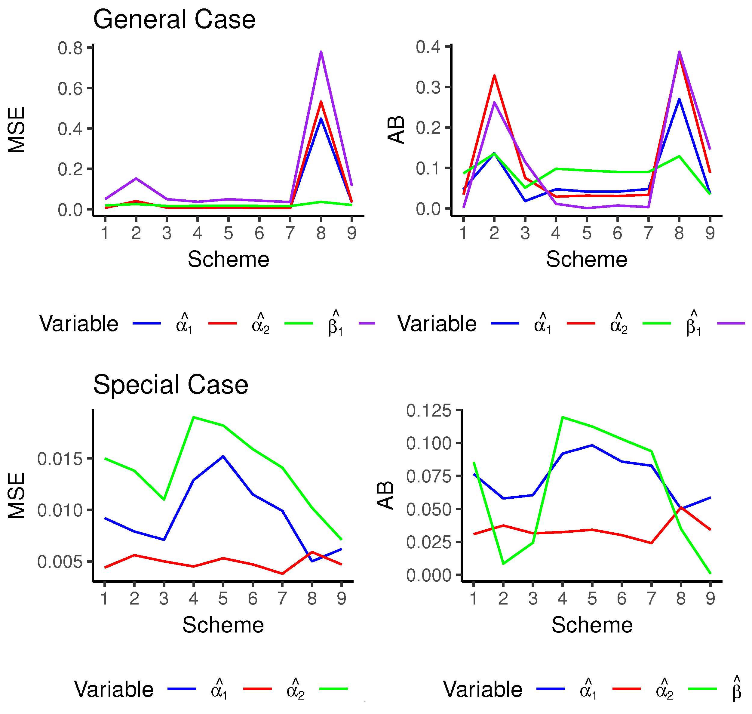
	$\beta$	0.5991	0.0071	0.0009	1.0000	0.9837

show the maximum likelihood estimates, the mean squared errors, the absolute biases and the empirical coverage probabilities (approximate and bootstrap) for the estimate of parameters for the general and special cases, respectively. For ease of comparison, the corresponding graphs are depicted in Figure 2. We observe that the estimation results are generally satisfactory in terms of MSEs and ABs for all censoring schemes. However, censoring schemes 3 and 9, which feature a uniform and smooth censoring of items, relatively outperformed other schemes in terms of both MSE and AB. Moreover, early censoring schemes (1, 4 and 7) performed better than other schemes with respect to the MSE with the same number of n and m. Also, note that relative risk due to cause 1 is given by $p={\displaystyle \frac{{\alpha }_2}{{\alpha }_1+{\alpha }_2}}=0.44$, meaning that, relatively, more data will be due to cause 2 rather than cause 1, resulting in a better estimate of the parameter ${\alpha }_2$, which is very clear in Figure 2.

Moreover, both confidence interval methods produce coverage probabilities of more than the nominated levels; however, the approximate confidence intervals performed better than the bootstrap ones.

Though this study focuses on the MLE approach, future work may compare its performance against Bayesian estimators or EM-type algorithms, particularly in the presence of model misspecification or small sample sizes.

6. Numerical Example

In this section, we study two numerical examples to illustrate our proposed inferential procedure for the Dagum Distribution.

Example 1 (Pneumonia data)

The data concerning investigating the impact of hospital-acquired infections in intensive care include a random subsample of 747 patients from the SIR 3 (Spread of Nosocomial Infections and Resistant Pathogens) cohort study conducted at Charité University Hospital in Berlin, Germany (see [42]). The data are also available in “mvna” R package.

The dataset includes details on pneumonia status at admission, duration of stay in the intensive care unit, and the ICU outcome, which is either hospital death or discharge alive. The competing endpoints are discharge from the unit and death within the unit.

The objective of the study is to examine the impact of pneumonia present at admission on mortality in the unit. Given that pneumonia is a severe illness, it is anticipated that more patients with pneumonia will die compared to those without. Thus, death is the primary event of interest, with discharge serving as the competing event.

Among the 97 patients admitted with pneumonia, 8 were censored before the end of their ICU stay. Therefore, we considered $n=89$ patients with pneumonia present on admission, of which 68 were discharged from hospital (failure cause 1) and 21 were dead (failure cause 2).

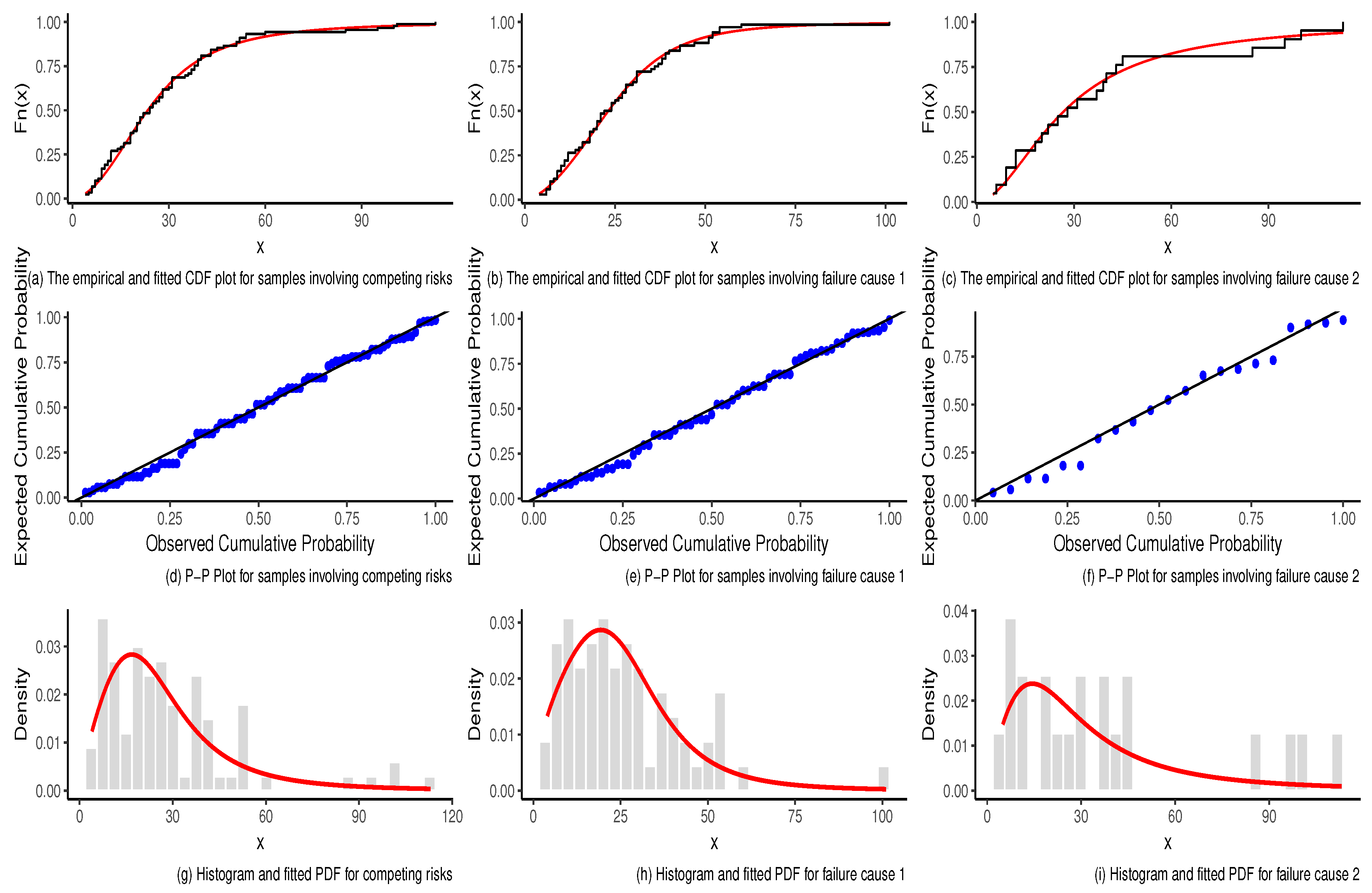
We checked the suitability of fitting the Dagum distribution to the competing risks, failure cause 1 and failure cause 2 data by performing well-known goodness-of-fit tests.

Table 4. The MLEs of the parameters, the gof test statistics and the corresponding p-values (in bracket) for the pneumonia data when testing for the Dagum distribution.

Failure Cause	$\widehat{\mathit{\alpha }}$	$\widehat{\mathit{\beta }}$	$\widehat{\mathit{\lambda }}$	${\mathit{\omega }}^2$ (p-Value)	D (p-Value)
Competing risk	0.65	2.76	29.54	0.0515 (0.8680)	0.0810 (0.6026)
Cause 1	0.43	3.71	33.68	0.0388 (0.9455)	0.0737 (0.8536)
Cause 2	0.98	1.91	27.01	0.0318 (0.9728)	0.1044 (0.9762)

provides the estimation of the parameters as well as the values of the Cramér–von Mises goodness-of-fit test statistic (${\omega }^2$) and the Kolmogorov–Smirnov statistic (D) with their corresponding p-values (in bracket) for the competing risk, failure cause 1 and failure cause 2. Note that $\lambda$ denoted the scale parameter of the general Dagum distribution. All the p-values are sufficiently large to conclude the suitability of the Dagum distribution to model the failure time data. Figure 3 depicts the plots of the empirical and fitted Dagum CDF for competing risks, cause 1 and cause 2 for pneumonia data. Additionally, it includes the P-P plot comparing observed cumulative probabilities with expected cumulative probabilities.

We then generated the progressive Type-II censoring data with effective sample size $m=50$ and the late censoring scheme $R=(0^{\ast }49,39)$ to complete the $n=89$ data. There were $m_1=40$ data due to failure cause 1 (discharge) and $m_2=10$ data due to failure cause 2 (death).

The test statistic for testing the null hypothesis $H_0:{\beta }_1={\beta }_2=\beta$ is equal to $T=21.98$ with a corresponding p-value $=0.00$, which is highly significant. Hence, we used the general model to estimate the unknown parameters.

Table 5. The point and interval estimates of the parameters for the pneumonia data under different censoring schemes.

Parameter	Scheme	MLE	Asymptotic CI	Bootstrap CI
	$R=(0^{\ast }49,39)$	0.4431	(0.3480, 0.5383)	(0.0649, 0.8064)
$\widehat{{\alpha }_1}$	$R=(39,0^{\ast }49)$	0.6174	(0.4889, 0.7460)	(0.1915, 0.9705)
	$R=(1^{\ast }39,0^{\ast }11)$	0.7237	(0.5622, 0.8852)	(0.5659, 1.1051)
	$R=(0^{\ast }49,39)$	1.2127	(0.9171, 1.5083)	(0.9203, 1.8105)
$\widehat{{\alpha }_2}$	$R=(39,0^{\ast }49)$	1.1567	(0.9515, 1.3618)	(0.8555, 1.5977)
	$R=(1^{\ast }39,0^{\ast }11)$	0.9763	(0.7611, 1.1915)	(0.6298, 1.2774)
	$R=(0^{\ast }49,39)$	3.6010	(3.4133, 3.8067)	(3.5409, 3.9979)
$\widehat{{\beta }_1}$	$R=(39,0^{\ast }49)$	3.6437	(2.9231, 4.3643)	(3.5010, 4.2016)
	$R=(1^{\ast }39,0^{\ast }11)$	3.9262	(3.6501, 4.2023)	(3.8772, 4.4468)
	$R=(0^{\ast }49,39)$	2.1934	(1.8898, 2.4970)	(1.9473, 2.5732)
$\widehat{{\beta }_2}$	$R=(39,0^{\ast }49)$	2.0785	(1.8786, 2.7357)	(1.4084, 2.8559)
	$R=(1^{\ast }39,0^{\ast }11)$	1.6731	(1.2871, 2.0591)	(1.2533, 2.1004)

shows the maximum likelihood estimates, the asymptotic confidence intervals and the bootstrap confidence intervals of the unknown parameters $({\alpha }_1,{\beta }_1)$ and $({\alpha }_2,{\beta }_2)$ under different censoring schemes for the failure causes 1 and 2, respectively. It can be seen that, in most cases, the asymptotic confidence intervals are shorter than the bootstrap confidence intervals, indicating superior performance in terms of length.

Example 2 (Leukemia data)

The dataset pertains to 177 acute leukemia patients who underwent stem cell transplantation. The competing risks are the incidence of relapse and death due to transplant-related complications. After excluding 46 censored cases, the dataset includes 131 patients, with 56 cases of relapse and 75 cases of competing events.

This dataset was analyzed by [43] to fit a competing risk regression model incorporating covariates such as age, gender, disease phase, and type of transplant. The data are available in “casebase” R package.

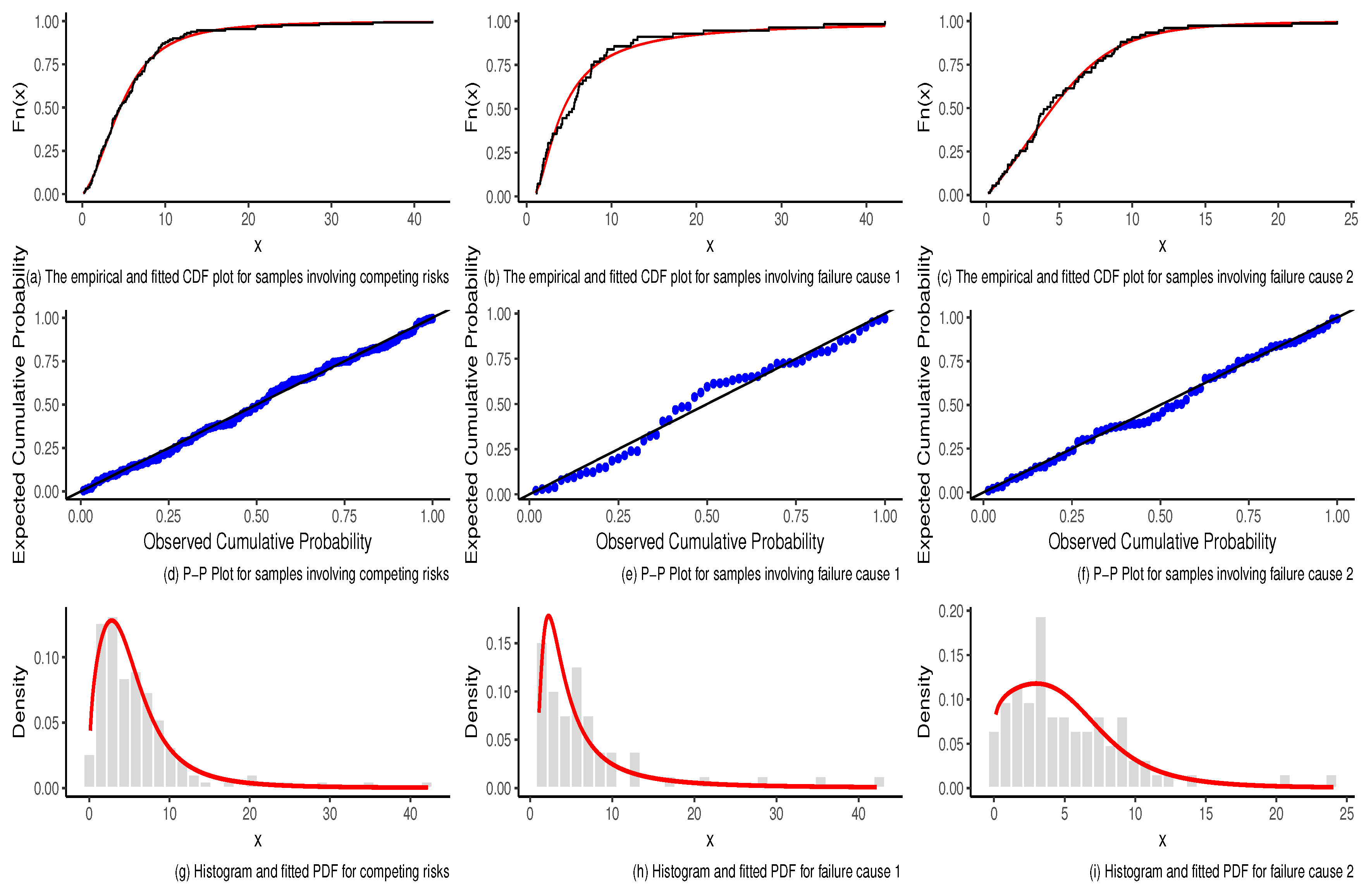
The results of the estimation of the parameters and the goodness-of-fit tests are shown in

Table 6. The MLEs of the parameters, the gof test statistics and the corresponding p-values (in brackets) for the leukemia data when testing for the Dagum distribution.

Failure Cause	$\widehat{\mathit{\alpha }}$	$\widehat{\mathit{\beta }}$	$\widehat{\mathit{\lambda }}$	${\mathit{\omega }}^2$ (p-Value)	D (p-Value)
Competing risk	0.55	2.55	6.57	0.0363 (0.9518)	0.0434 (0.9657)
Cause 1	6.65	1.44	0.94	0.1119 (0.5312)	0.1161 (0.4369)
Cause 2	0.31	3.62	8.14	0.0353 (0.9568)	0.0589 (0.9571)

. As observed, the null hypothesis that the data for the failure cause 1, failure cause 2 and competing risk follow a Dagum distribution is not rejected for any of the three test statistics.

Figure 4 depicts the plots of the empirical CDF, fitted Dagum CDF and P-P plot for competing risks, cause 1 and cause 2 for the leukemia data.

Progressive Type-II censoring data were generated with an effective sample size of $m=40$ using the early censoring scheme $R=(91,0^{\ast }39)$ applied to a complete dataset of size $n=131$. The resulting data included $m_1=18$ observations attributed to failure cause 1 (relapse) and $m_2=22$ observations due to competing events. Note that the sample size $m=40$ is below the conventional threshold for large-sample inference. Therefore, we recommend relying on bootstrap-based intervals to ensure accurate uncertainty quantification.

We test for for the null hypothesis of the equality of shape 2 parameters ${\beta }_1$ and ${\beta }_2$. The test statistic was found to be $T=13.32$ with a p-value equal to 0.003, indicating a high level of significance. Hence, we considered the general case for estimating the parameters.

Table 7. The point and interval estimates of the parameters for the Leukemia data under different censoring schemes.

Parameter	Scheme	MLE	Asymptotic CI	Bootstrap CI
	$R=(0^{\ast }39,91)$	0.7151	(0.5527, 0.8776)	(0.7705, 0.9721)
$\widehat{{\alpha }_1}$	$R=(91,0^{\ast }39)$	0.6406	(0.5539, 0.7272)	(0.5467, 0.8498)
	$R=(3^{\ast }30,1,0^{\ast }9)$	0.9020	(0.7144, 1.0896)	(0.7444, 1.3072)
	$R=(0^{\ast }39,91)$	0.8632	(0.6911, 1.0352)	(0.7383, 0.9778)
$\widehat{{\alpha }_2}$	$R=(91,0^{\ast }39)$	1.4165	(1.2937, 1.5393)	(1.1491, 1.8382)
	$R=(3^{\ast }30,1,0^{\ast }9)$	0.5019	(0.4129, 0.5907)	(0.0809, 0.8638)
	$R=(0^{\ast }39,91)$	3.9742	(3.6741, 4.0743)	(3.9771, 4.2053)
$\widehat{{\beta }_1}$	$R=(91,0^{\ast }39)$	3.7955	(3.2697, 4.3213)	(3.9015, 4.1460)
	$R=(3^{\ast }30,1,0^{\ast }9)$	3.9700	(3.4949, 4.4451)	(4.0222, 4.5507)
	$R=(0^{\ast }39,91)$	1.8320	(1.7128, 1.9513)	(1.7341, 2.0731)
$\widehat{{\beta }_2}$	$R=(91,0^{\ast }39)$	1.4426	(0.7436, 2.1417)	(1.0814, 1.9950)
	$R=(3^{\ast }30,1,0^{\ast }9)$	1.9609	(1.7351, 2.1867)	(1.6369, 2.2743)

presents the maximum likelihood estimates and the asymptotic and bootstrap confidence intervals of the unknown parameters when considering various censoring schemes.

It can be seen that, in most cases, the asymptotic confidence intervals are shorter than the bootstrap confidence intervals when estimating ${\alpha }_1$ and ${\alpha }_2$. However, for estimating ${\beta }_1$ and ${\beta }_2$, the bootstrap confidence intervals are shorter and thus perform better in terms of length.

As shown in Table 7, the asymptotic confidence intervals are generally shorter than the bootstrap confidence intervals for estimating ${\alpha }_1$ and ${\alpha }_2$, except under the conventional Type-II censoring scheme, where the bootstrap confidence intervals are shorter. For ${\beta }_1$, the bootstrap confidence intervals consistently outperform the asymptotic confidence intervals across all schemes in terms of length. In contrast, for ${\beta }_2$, the asymptotic confidence intervals are shorter than the bootstrap confidence intervals under the conventional Type-II censoring scheme and the third smoothing censoring scheme.

7. Concluding Remarks

This paper proposes statistical inference methods to estimate the parameters of the Dagum distribution under progressively Type-II censored data with independent competing risks, including both point and interval estimation. Monte Carlo simulations demonstrate that the proposed methods perform relatively well. The interval estimation obtained from the asymptotic model generally outperforms the bootstrap method. Different censoring schemes affect both point and interval estimation, with early censoring schemes yielding the best results. Moreover, the conventional Type-II censoring scheme performs relatively well. The special case of common shape parameter $\beta$ yields to a closed form for the reliability parameter $R=P(X_{1j}<X_{2j})$ in Remark 1. For a general setting of different values of ${\beta }_1$ and ${\beta }_2$, the reliability parameter R is given by the following:

$$R={\alpha }_1{\beta }_1{\int }_0^{\infty }{(1+x^{-{\beta }_2})}^{-{\alpha }_2}{x}^{-({\beta }_1+1)}{(1+x^{-{\beta }_1})}^{-({\alpha }_1+1)}dx.$$

It is evident that a numerical method is required to evaluate this integral. While this paper focuses on the case $k=2$, extending our methods to systems with more than two failure modes substantially increases the dimensionality of the likelihood functions and, therefore, finding the maximum likelihood estimators becomes more challenging.

For future work, one could consider dependent failure models by fitting a bivariate distribution, such as the bivariate exponential model or bivariate Dagum distribution (see [44]). Additionally, other censoring schemes, such as hybrid censoring, can be explored.

Moreover, future studies could include the incorporation of covariates using regression models, the development of Bayesian estimation procedures, or the modeling of dependent competing risks via bivariate Dagum or copula-based methods. To enhance reproducibility, the R code used for simulations and data analysis is available upon request.