Modified Bimodal Exponential Distribution with Applications

Abstract

In this paper, we introduce a new distribution for modeling bimodal data supported on non-negative real numbers and particularly suited with an excess of very small values. This family of distributions is derived by multiplying the exponential distribution by a fourth-degree polynomial, resulting in a model that better fits the shape of the second mode of the empirical distribution of the data. We study the general density of this new family of distributions, along with its properties, moments, and skewness and kurtosis coefficients. A simulation study is performed to estimate parameters by the maximum likelihood method. Additionally, we present two applications to real-world datasets, demonstrating that the new distribution provides a better fit than the bimodal exponential distribution.

1. Introduction

Weighted distributions frequently occur in research related to survival analysis, analysis of intervention data, ecology and biomedicine, and other areas. Fisher [1] and Rao [2] introduced the concept of weighted distributions to improve the fit of appropriate statistical models; this idea has been used to select an appropriate model for the data observed (see Rao [3]). A random variable Y follows the weighted distribution if its probability density function (pdf) is given by

$$\begin{array}{c}\hfill {\displaystyle ll{f}_Y\left(y\right)=\frac{w\left(y\right)f\left(y\right)}{E\left(w\right(Y\left)\right)},}\end{array}$$

(1)

where f is a density function, and w is a positive function. Analysis and applications using this methodology can be found in Patil and Ord [4], Patil and Rao [5], Gupta and Kirmani [6], Gupta and Tripathi [7], Gupta and Akman [8], Gupta and Kundu [9], Reyes et al. [10], Hassan and Hijazi [11], Gómez-Déniz et al. [12], Chesneau et al. [13], Alzaghal et al. [14], Cortés et al. [15], and others.

Reyes et al. [10] considered the exponential model, $f\left(y\right)=\alpha e^{-\alpha y}$, and the weight function $w\left(y\right)={\left(1-q\alpha \left(y-{\displaystyle \frac{1}{\alpha }}\right)\right)}^2+1$; using (1) they constructed and study the bimodal exponential (BE) distribution, the pdf of which is given by

$$\begin{array}{c}\hfill f_Y(y;\alpha ,q)={\displaystyle \frac{\alpha }{2+q^2}}\left[{\left(1-q\alpha \left(y-{\displaystyle \frac{1}{\alpha }}\right)\right)}^2+1\right]e^{-\alpha y},y\ge 0,\end{array}$$

(2)

with $\alpha >0$ and $q\in \mathbb{R}$. It is denoted by $Y\sim BE(\alpha ,q)$. The BE distribution is bimodal and is an extension of the exponential distribution. Furthermore, it can be used to fit datasets containing zeroes and/or very small values. The motivation for studying these families of bimodal distributions stems from the lack of alternative models that can effectively replace mixture distributions, which—as is well known—present estimation problems when using classical approaches like Bayesian methods (see McLachan and Peel [16]; Marin et al. [17]).

The object of the present work is to modify the BE distribution considering a new function $w(·)$ which increases the flexibility of the second mode. We thus obtain a modified bimodal exponential (MBE) distribution, which we denote by $Y\sim MBE(\alpha ,q)$. We study its properties, estimating the parameters, and compare it with the BE distribution using a real dataset.

The work is organized as follows. In Section 2, we present the pdf of the MBE distribution and study some of its properties. In Section 3, we study the inferential statistics of the MBE distribution, in particular the moments estimators and maximum likelihood (ML) estimators, and present a simulation study. In Section 4, we present two applications to real-world datasets. Finally, Section 5 provides concluding remarks.

2. Density and Properties

In this section, we present the pdf of the MBE distribution and some of its properties.

Proposition 1.

Let $Y\sim MBE(\alpha ,q)$. Then, the density function of Y is given by

$$\begin{array}{c}\hfill f_Y\left(y\right)={\displaystyle \frac{\alpha }{1+9q}}\left(1+q{\alpha }^4{\left(y-{\displaystyle \frac{1}{\alpha }}\right)}^4\right)e^{-\alpha y},y\ge 0,\end{array}$$

(3)

with $\alpha >0$ defining the rate parameter and $q\ge 0$ defining the shape parameter.

Proof. 

Considering $f\left(y\right)=\alpha e^{-\alpha y}$, $w\left(y\right)=1+q{\alpha }^4{\left(y-{\displaystyle \frac{1}{\alpha }}\right)}^4$, and using (1), we obtain the result.

   □

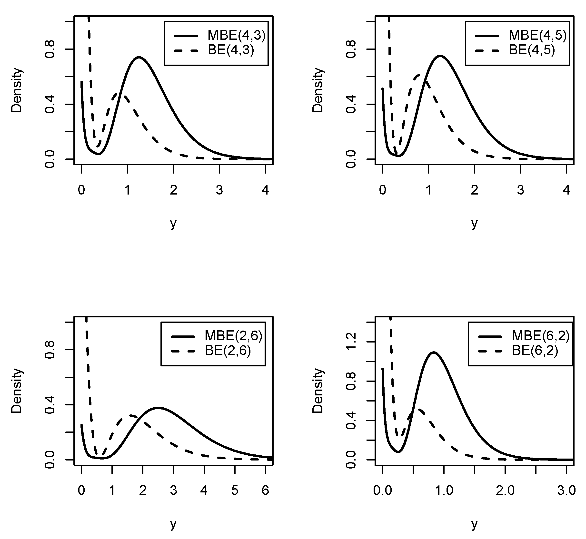
Below, we illustrate graphically the behavior of the density function of the MBE distribution, comparing it with the BE distribution.

Remark 1.

We observe that the MBE can be used to model datasets with an excess of zeroes or very small values, as its support includes zero, and it possesses a mode at zero. We likewise observe that when the parameter $q=0$, the exponential distribution is obtained as a particular case.

Proposition 2.

Let $Y\sim MBE(\alpha ,q)$. The solutions of

$$\begin{array}{c}\hfill q{(\alpha y-1)}^4-4q{(\alpha y-1)}^3+1=0,\end{array}$$

(4)

correspond to the anti-mode and the non-zero mode of the distribution of Y.

Proof. 

This follows directly from analyzing the first derivative of (1) with respect to y.    □

The quartic equation in (4) can be solved analytically using the Cardano–Ferrari formulas (for details, see Abramowitz and Stegun [18]). For numerical solutions, the WolframAlpha computational platform (https://www.wolframalpha.com/) provides an efficient alternative; for more details we refer the reader to Weisstein [19].

Let $Z\sim BE(\alpha ,q)$, and let $Y\sim MBE(\alpha ,q)$.

Table 1. Values of the second modes of the BE and MBE distributions.

$\mathit{\alpha }$	q	Modes
4	3	$M_0\left(Z\right)\approx 0.8190$
		$M_0\left(Y\right)\approx 1.2487$
4	5	$M_0\left(Z\right)\approx 0.7950$
		$M_0\left(Y\right)\approx 1.2492$
2	6	$M_0\left(Z\right)\approx 1.5763$
		$M_0\left(Y\right)\approx 2.4987$
6	2	$M_0\left(Z\right)\approx 0.5610$
		$M_0\left(Y\right)\approx 0.8320$

shows the values of the modes for the BE and MBE distributions with the same parameter values as in Figure 1.

Proposition 3.

Let $Y\sim MBE(\alpha ,q)$ and $Z\sim BE(\alpha ,q)$. Then, the height of the second mode of Y is greater than the height of the second mode of Z for $1\le q\le 25.34$, where the second mode of Y is between ${\displaystyle \frac{4}{\alpha }}$ and ${\displaystyle \frac{5}{\alpha }}$, and Z becomes $M_0\left(Z\right)={\displaystyle \frac{1+2q+\sqrt{q^2-1}}{\alpha q}}$.

Proof. 

For $q\ge 1$, the second mode of Z is given by $M_0\left(Z\right)={\displaystyle \frac{1+2q+\sqrt{q^2-1}}{\alpha q}}$ (see Reyes et al. [10]). The first derivative of $f_Y\left(y\right)$ is given by

$$f_Y^{\prime }\left(y\right)=-{\displaystyle \frac{{\alpha }^2}{1+9q}}(q{(\alpha y-1)}^4-4q{(\alpha y-1)}^3+1)e^{-\alpha y}.$$

Evaluating this at $y={\displaystyle \frac{4}{\alpha }}$ and $y={\displaystyle \frac{5}{\alpha }}$ yields

$$f_Y^{\prime }\left({\displaystyle \frac{4}{\alpha }}\right)=-{\displaystyle \frac{{\alpha }^2}{1+9q}}(1-27q)e^{-4}>0and{f}_Y^{\prime }\left({\displaystyle \frac{5}{\alpha }}\right)=-{\displaystyle \frac{{\alpha }^2}{1+9q}}{e}^{-5}<0.$$

Thus, ${\displaystyle \frac{4}{\alpha }}<M_0\left(Y\right)<{\displaystyle \frac{5}{\alpha }}$, which implies that the height of the second mode of Y is greater than $f_Z\left({\displaystyle \frac{5}{\alpha }}\right)$. Furthermore, we calculate

$$f_Z\left({\displaystyle \frac{3}{\alpha }}\right)=\alpha {\displaystyle \frac{2-4q+4q^2}{2+q^2}}{e}^{-3}and{f}_Y\left({\displaystyle \frac{5}{\alpha }}\right)={\displaystyle \frac{\alpha }{1+9q}}(1+256q)e^{-5}.$$

The inequality $f_Y\left({\displaystyle \frac{5}{\alpha }}\right)\ge f_Z\left({\displaystyle \frac{3}{\alpha }}\right)$ holds for $1\le q\le 25.34$, as established by solving

$$(256e^{-2}-36)q^3+(e^{-2}+32)q^2+(512e^{-2}-14)q+2(e^{-2}-1)\ge 0.$$

Since $f_Y\left(M_0\left(Y\right)\right)>f_Y\left({\displaystyle \frac{5}{\alpha }}\right)$, the proof is complete.   □

Proposition 4.

Let $Y\sim MBE(\alpha ,q)$. Then, the cumulative distribution function (cdf) of Y is given by

$$\begin{array}{ccc}\hfill F_Y\left(y\right)& =& 1-{\displaystyle \frac{e^{-\alpha y}}{1+9q}}\left[\alpha qy({\alpha }^3{y}^3+6\alpha y+8)+(1+9q)\right].\hfill \end{array}$$

(5)

Proof. 

Calculating directly from the definition of the cdf, we have

$$F_Y\left(y\right)={\int }_0^y{f}_Y\left(u\right)du={\int }_0^y{\displaystyle \frac{\alpha }{1+9q}}\left(1+q{\alpha }^4{\left(u-{\displaystyle \frac{1}{\alpha }}\right)}^4\right)e^{-\alpha u}du,$$

and the result is obtained by developing the integral.    □

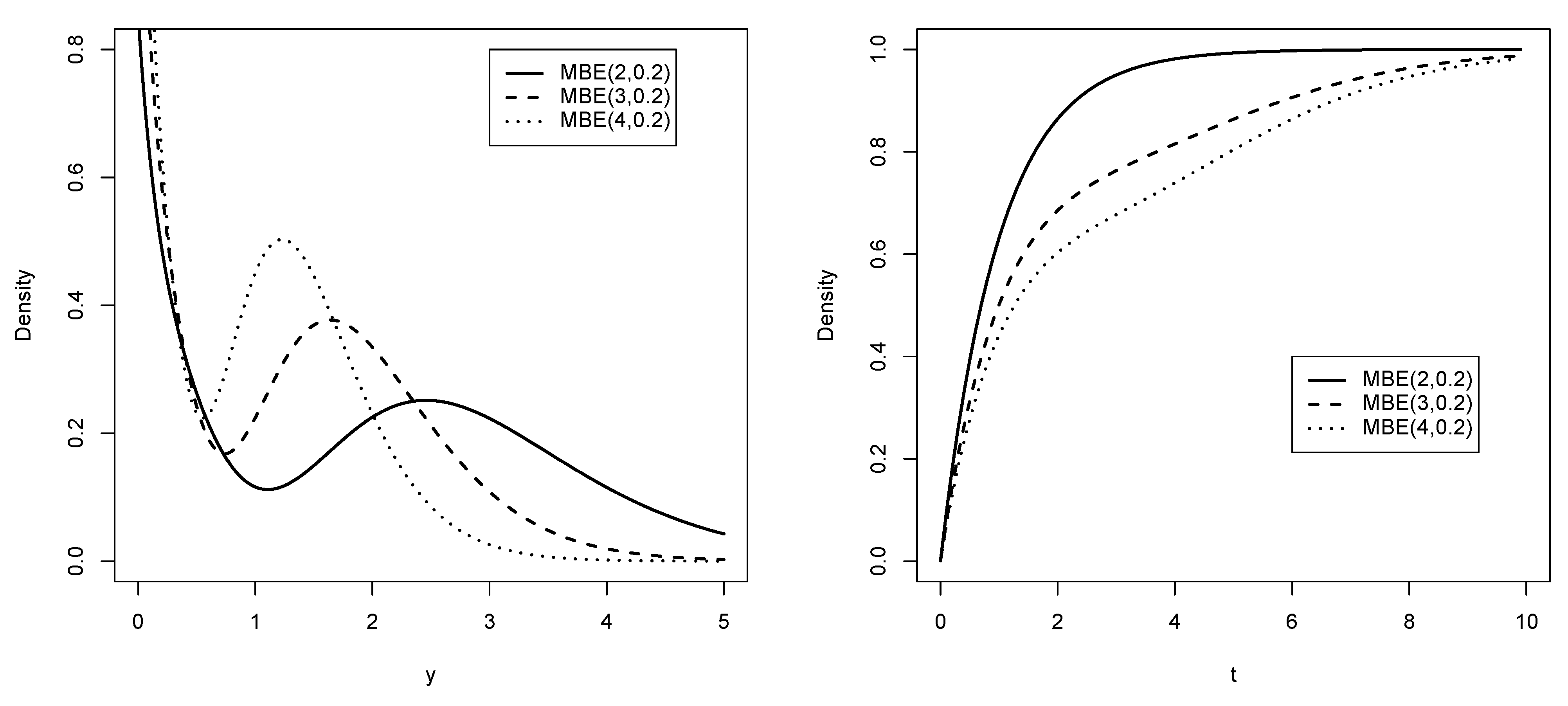
Remark 2.

The BE distribution has a unique mode at zero when $q<1$ (see Reyes et al. [10]); otherwise, like the MBE distribution, it has two modes, as shown in Figure 2. The MBE distribution always has two modes: one at zero and another at a point $x_0>0$, with the latter having a greater height.

Below, we illustrate graphically the behavior of the pdf and cdf of the MBE distribution.

Figure 2. Pdf and cdf for the MBE distribution for values of $\alpha$ and q.

Figure 2. Pdf and cdf for the MBE distribution for values of $\alpha$ and q.

2.1. Order Statistics

Let $Y_1,\dots ,Y_n$ be a random sample of the random variable $Y\sim MBE(\alpha ,q)$; let us denote by $Y_{\left(j\right)}$ the $jth-$ order statistics $j\in \{1,\dots ,n\}$.

Proposition 5.

The pdf of $Y_{\left(j\right)}$ is

$$\begin{array}{cc}\hfill f_{Y_{\left(j\right)}}\left(y\right)& ={\displaystyle \frac{n!\alpha \left(1+q{(\alpha y-1)}^4\right)e^{-\alpha y(n-j+1)}}{(j-1)!(n-j)!{(1+9q)}^n}}{\left\{1+9q-e^{-\alpha y}\left(\alpha qy({\alpha }^3{y}^3+6\alpha y+8)+1+9q\right)\right\}}^{j-1}\\ \times {\left\{\alpha qy({\alpha }^3{y}^3+6\alpha y+8)+1+9q\right\}}^{n-j},y>0.\end{array}$$

In particular, the pdf of the minimum, $Y_{\left(1\right)}$, is

$$f_{Y_{\left(1\right)}}\left(y\right)={\displaystyle \frac{n\alpha \left(1+q{(\alpha y-1)}^4\right)e^{-n\alpha y}}{{(1+9q)}^n}}{\left\{\alpha qy({\alpha }^3{y}^3+6\alpha y+8)+1+9q\right\}}^{n-1},y>0.$$

and the pdf of the maximum, $Y_{\left(n\right)}$, is

$$f_{Y_{\left(n\right)}}\left(y\right)={\displaystyle \frac{n\alpha \left(1+q{(\alpha y-1)}^4\right)e^{-\alpha y}}{{(1+9q)}^n}}{\left\{1+9q-e^{-\alpha y}\left(\alpha qy({\alpha }^3{y}^3+6\alpha y+8)+1+9q\right)\right\}}^{n-1},y>0.$$

Proof. 

Since we are dealing with an absolutely continuous model, the pdf of the $jth-$ order statistics is obtained by applying

$$\begin{array}{ccc}\hfill f_{Y_{\left(j\right)}}\left(y\right)& =& {\displaystyle \frac{n!}{(j-1)!(n-j)!}}f\left(y\right){\left[F\left(y\right)\right]}^{j-1}{[1-F\left(y\right)]}^{n-j},j\in \{1,\dots ,n\}\hfill \end{array}$$

where F and f denote the cdf and pdf of the parent distribution, $Y\sim MBE(\alpha ,q)$, in this case. More precisely, substituting Equations (3) and (5) yields the result.    □

2.2. The Reliability and Hazard Rate Functions

Two important reliability measures are the reliability function and the hazard (failure) rate function. The reliability function of a random variable Y is defined by $R_Y\left(t\right)=1-F_Y\left(t\right)$, where $F_Y$ denotes the cdf of Y. The hazard rate function is defined by $h_Y\left(t\right)=f_Y\left(t\right)/(1-F_Y\left(t\right))$. For the BE distribution, as a direct consequence of Proposition 1 and Proposition 2, both reliability measures can be expressed in closed form. The corresponding expressions are obtained in a straightforward manner.

Proposition 6.

Let $Y\sim MBE(\alpha ,q)$. Then, the hazard function of Y is given by

$$\begin{array}{ccc}\hfill h\left(t\right)& =& {\displaystyle \frac{\alpha \left[1+q{\left(\alpha t-1\right)}^4\right]}{\alpha qt({\alpha }^3{t}^3+6\alpha t+8)+1+9q}}.\hfill \end{array}$$

(6)

Proof. 

By definition of the hazard function, we have

$$\begin{array}{c}\hfill h_Y\left(t\right)=f_Y\left(t\right)/(1-F_Y\left(t\right)),\end{array}$$

and then by replacing $f_Y\left(t\right)$ and $F_Y\left(t\right)$, the result is obtained.    □

To prove the following proposition, we will use the theorem in Glaser [20], together with the idea that to study the behavior of the harzard function $h\left(t\right)$, we can examine the function $\eta \left(t\right)$ defined by $\eta \left(t\right)=-f^{\prime }\left(t\right)/f\left(t\right)$, where $f\left(t\right)$ is the pdf given in (1).

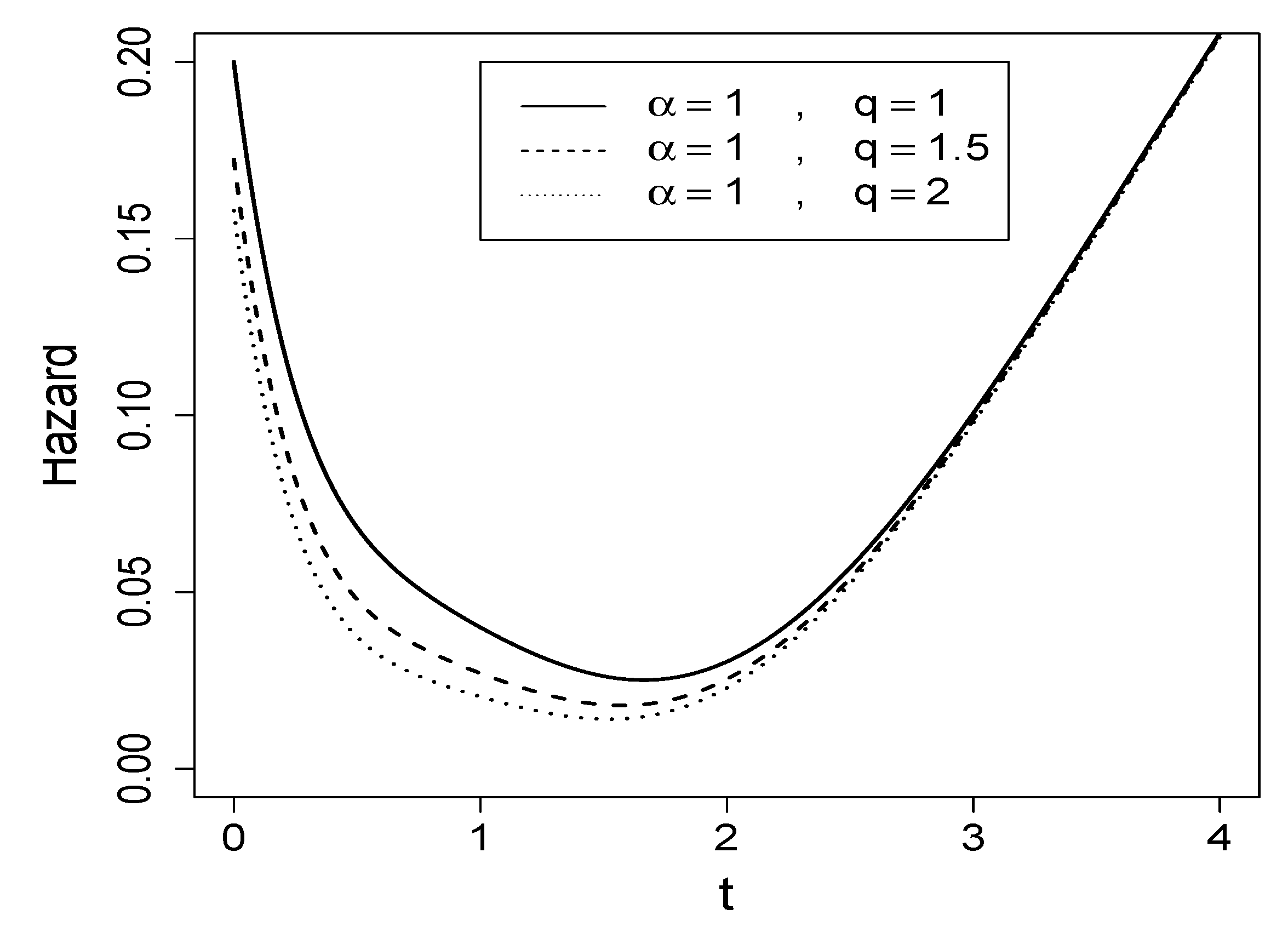
Proposition 7.

Let $T\sim MBE(\alpha ,q)$. Then, the hazard function of T has a bathtub shape.

Proof. 

Using item $c)$ of Glaser’s Theorem [20], we define the functions

$$\begin{array}{c}\hfill \eta \left(t\right)=\alpha -{\displaystyle \frac{4\alpha q{(\alpha t-1)}^3}{1+q{(\alpha t-1)}^4}},\end{array}$$

and the function $g\left(t\right)=1/h\left(t\right)$. Their first derivatives are, respectively,

$$\begin{array}{c}\hfill {\eta }^{\prime }\left(t\right)={\displaystyle \frac{4{\alpha }^{2}q{(\alpha t-1)}^2\left(q{(\alpha t-1)}^4-3\right)}{{\left(1+q{(\alpha t-1)}^4\right)}^2}},and{g}^{\prime }\left(t\right)=\eta \left(t\right)/h\left(t\right)-1.\end{array}$$

If $q\le 3$, we obtain the following: ${\eta }^{\prime }\left(t\right)<0$ in $t\in (0,t_0)$, ${\eta }^{\prime }\left(t_0\right)=0$, and ${\eta }^{\prime }\left(t\right)>0$ for all $t>t_0$ when $t_0={\displaystyle \frac{1}{\alpha }}\left(1+\sqrt[4]{{\displaystyle \frac{3}{q}}}\right)$.

On the other hand, we observe that as $t\to 0^{+}$, $h\left(t\right)\to \alpha (1+q)/(1+9q)$, and $\eta \left(t\right)\to \alpha (1+5q)/(1+q)$, which implies that $\eta \left(t\right)>h\left(t\right)$ as $t\to 0^{+}$. Additionally, evaluating these functions at $t_0$, we have

$$h\left(t_0\right)={\displaystyle \frac{\alpha }{6\sqrt[4]{3q^3}+\sqrt[4]{27q}+3\sqrt{3q}+6q+1}}and\eta \left(t_0\right)=\alpha (1-\sqrt[4]{27q}),$$

yielding $\eta \left(t_0\right)<h\left(t_0\right)$. Since $\eta -h$ is a continuous function for all t, there exists $y_0<t_0$ such that $\eta \left(y_0\right)=h\left(y_0\right)$. Consequently, $g^{\prime }\left(y_0\right)=0$; by applying item $c)$ of Glaser’s Theorem [20], the result follows.

If $q>3$, ${\eta }^{\prime }$ is null at three points:

$$t_1={\displaystyle \frac{1}{\alpha }}\left(1-\sqrt[4]{{\displaystyle \frac{3}{q}}}\right),t_2={\displaystyle \frac{1}{\alpha }}and{t}_3={\displaystyle \frac{1}{\alpha }}\left(1+\sqrt[4]{{\displaystyle \frac{3}{q}}}\right).$$

This is because

$${\eta }^{\prime \prime }\left(t_3\right)=3\alpha \sqrt[4]{3q^3}>0.$$

Since $\eta \left(t\right)$ has a local minimum at $t_3$, the hazard function also attains a local minimum at $t_3$, resulting in a bathtub-shaped hazard function.    □

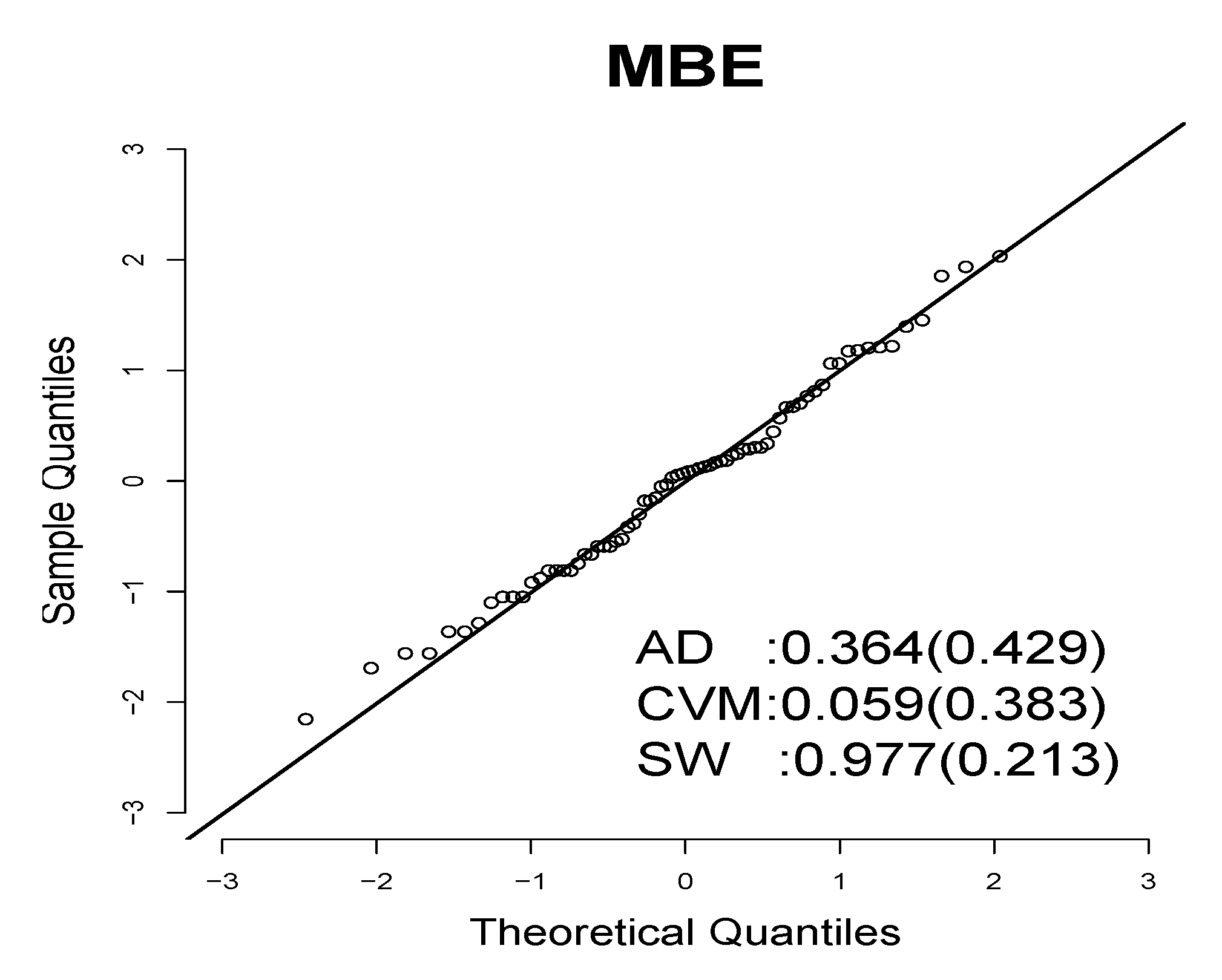
Figure 3 presents the hazard rate function of the MBE distribution for various parameter configurations. Notably, the hazard function exhibits the characteristic bathtub shape, a feature frequently encountered in reliability and survival analysis.

2.3. Moments

The moments of a random variable with modified bimodal exponential distribution are given in the following proposition.

Proposition 8.

If $Y\sim MEB(\alpha ,q)$, the r-th moment of Y is given by

$$\begin{array}{ccc}\hfill {\mu }_r=\mathbb{E}\left[Y^r\right]& =& {\displaystyle \frac{r!}{{\alpha }^r(1+9q)}}[1+q(r^4+6r^3+17r^2+20r+9)].\hfill \end{array}$$

(7)

Proof. 

Calculating directly from the definition, we have

$${\mu }_r=\mathbb{E}\left[Y^r\right]={\int }_0^{\infty }{\displaystyle \frac{y^r}{1+9q}}\left(1+q{\left(\alpha y-1\right)}^4\right)\alpha e^{-\alpha y}dy.$$

The result is obtained by developing the integral.    □

Corollary 1.

Let $Y\sim MEB(\alpha ,q)$; then,

$$\begin{array}{cc}\hfill {\mu }_1=\mathbb{E}\left(Y\right)={\displaystyle \frac{1}{\alpha (1+9q)}}(1+53q),& {\mu }_2=\mathbb{E}\left(Y^2\right)={\displaystyle \frac{2}{{\alpha }^2(1+9q)}}(1+181q),\\ \hfill {\mu }_3=\mathbb{E}\left(Y^3\right)={\displaystyle \frac{6}{{\alpha }^3(1+9q)}}(1+465q),& {\mu }_4=\mathbb{E}\left(Y^4\right)={\displaystyle \frac{24}{{\alpha }^4(1+9q)}}(1+1001q).\end{array}$$

Proof. 

This is an immediate consequence of the previous proposition.    □

Corollary 2.

Let $Y\sim MBE(\alpha ,q)$; then, the expectation and the variance of Y are given by

$$\mathbb{E}\left(Y\right)={\displaystyle \frac{1}{\alpha (1+9q)}}(1+53q),andVar\left(Y\right)={\displaystyle \frac{1}{{\alpha }^2{\left(9q+1\right)}^2}}\left(449q^2+274q+1\right).$$

Corollary 3.

Let $Y\sim MBE(\alpha ,q)$; then, the asymmetry coefficient (${\beta }_1$) and the kurtosis coefficient (${\beta }_2$) of Y are given by

$${\beta }_1={\displaystyle \frac{5722q^3-2634q^2+1758q+2}{{\left(449q^2+274q+1\right)}^{\frac{3}{2}}}},and{\beta }_2={\displaystyle \frac{842,505q^4+891,780q^3+81,654q^2+14,724q+9}{{\left(449q^2+274q+1\right)}^2}},$$

respectively.

Proof. 

Using the expressions obtained in the previous corollary and the following equations, the result is obtained as

$${\beta }_1={\displaystyle \frac{\mathbb{E}{\left[Y-\mathbb{E}\left(Y\right)\right]}^3}{{\left[\mathrm{Var}\left(Y\right)\right]}^{3/2}}}={\displaystyle \frac{{\mu }_3-3{\mu }_2{\mu }_1+2{\mu }_1^3}{{({\mu }_2-{\mu }_1^2)}^{3/2}}},$$

and

$${\beta }_2={\displaystyle \frac{\mathbb{E}{\left[Y-\mathbb{E}\left(Y\right)\right]}^4}{{\left[\mathrm{Var}\left(Y\right)\right]}^2}}={\displaystyle \frac{{\mu }_4-4{\mu }_1{\mu }_3+6{\mu }_1^2{\mu }_2-3{\mu }_1^4}{{({\mu }_2-{\mu }_1^2)}^2}},$$

respectively.    □

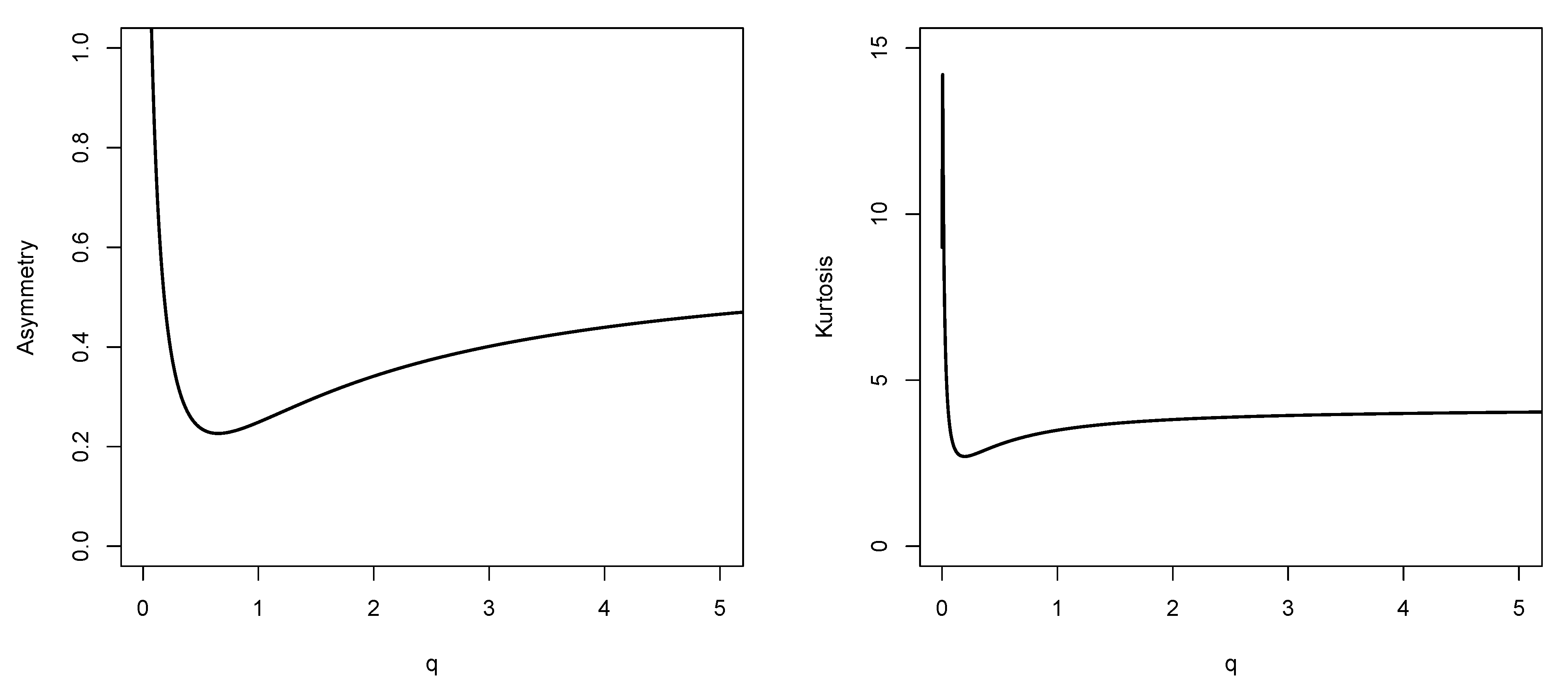
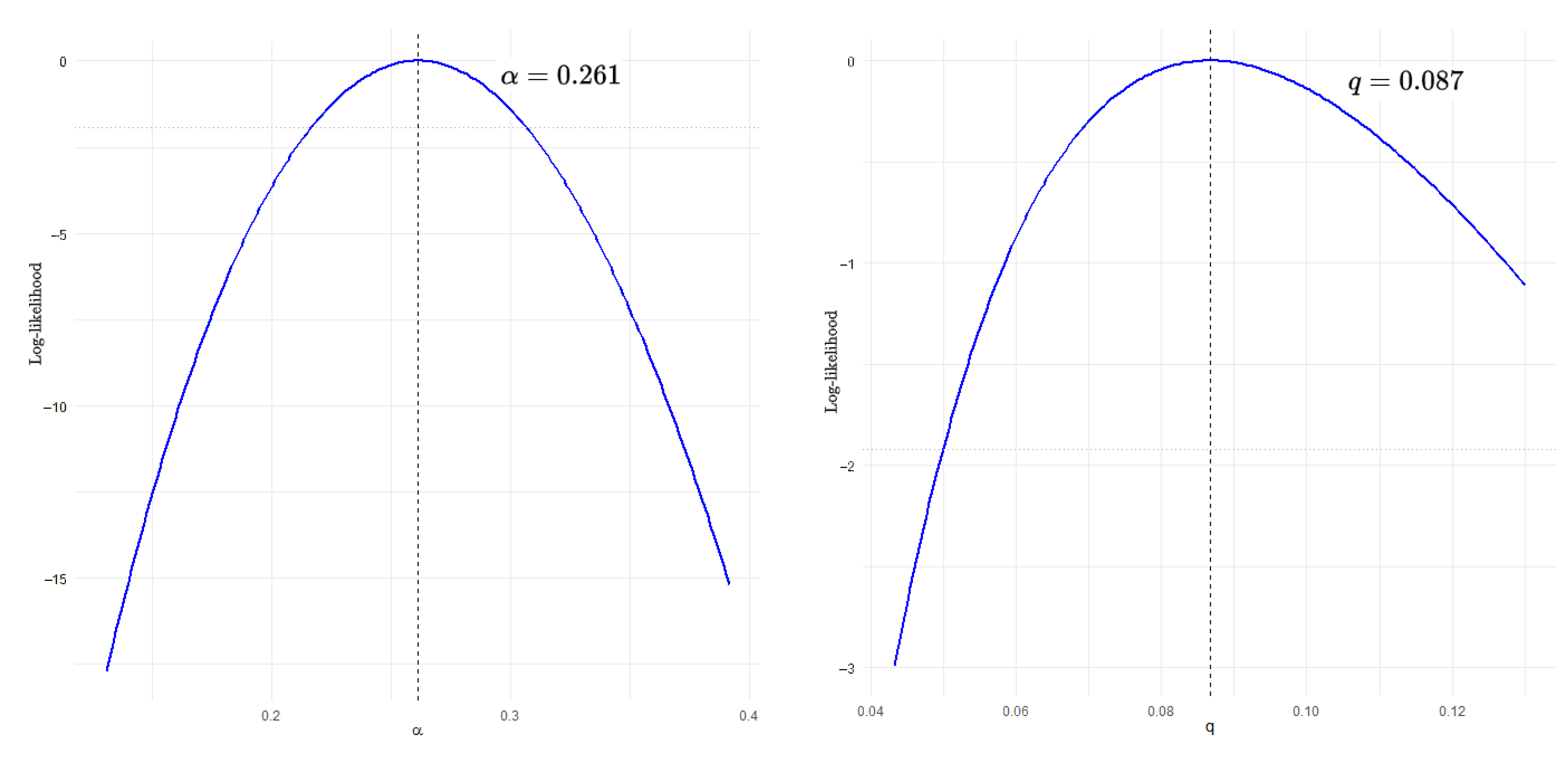
Figure 4 shows the skewness and kurtosis coefficients as a function of the parameter q for the MBE model.

Proposition 9.

Let $Y\sim MBE(\alpha ,q)$. Then, the moment generating function for $\alpha >t$ is given by

$$\begin{array}{c}\hfill M_Y\left(t\right)={\displaystyle \frac{\alpha }{1+9q}}\left\{{(\alpha -t)}^{-1}+q\left[{(\alpha -t)}^{-1}-4\alpha {(\alpha -t)}^{-2}+12{\alpha }^2{(\alpha -t)}^{-3}+24{\alpha }^{3}t{(\alpha -t)}^{-5}\right]\right\}\end{array}$$

Proof. 

Calculating directly from the definition, we have

$$M_Y\left(t\right)=\mathbb{E}\left(e^{tY}\right)={\displaystyle \frac{\alpha }{1+9q}}{\int }_0^{\infty }\left(1+q{(\alpha y-1)}^4\right)e^{-(\alpha -t)y}dy,$$

and then, the result is obtained by calculating the integral for $\alpha >t$.    □

3. Inference

In this section, we discuss statistical inferences from the moment estimators and maximum likelihood estimators.

3.1. Moment Estimators

Proposition 10.

Let $Y_1,\dots ,Y_n$ be a random distributed sample defined as $Y\sim MBE(\alpha ,q)$. Then, the moment estimators $({\widehat{\alpha }}_M,{\widehat{q}}_M)$ of $(\alpha ,q)$ are as follows:

$${\widehat{\alpha }}_M={\displaystyle \frac{1+53{\widehat{q}}_M}{\overline{Y}(1+9{\widehat{q}}_M)}},$$

(8)

$${\widehat{q}}_M={\displaystyle \frac{190{\overline{Y}}^2-53\overline{Y^2}+4\overline{Y}\sqrt{1849{\overline{Y}}^2-704\overline{Y^2}}}{2809\overline{Y^2}-3258{\overline{Y}}^2}},$$

(9)

where $1849{\overline{Y}}^2\ge 704\overline{Y^2}$, the value of ${\widehat{q}}_M$ found is replaced in (8), and ${\widehat{\alpha }}_M$ is obtained.

Proof. 

From Proposition 8 and using the first two equations and following the moments method, we have

$$\overline{Y}={\displaystyle \frac{1+53q}{\alpha (1+9q)}},\overline{Y^2}={\displaystyle \frac{2(1+181q)}{{\alpha }^2(1+9q)}},$$

solving the first equation above for $\alpha$, we obtain ${\widehat{\alpha }}_M$ given in (8). Substituting ${\widehat{\alpha }}_M$ in the second equation above, we obtain the result given in (9).    □

3.2. ML Estimation

We now discuss ML estimation. Given a random sample $Y_1,\dots ,Y_n$ from the distribution of MBE($\alpha ,q$), the log likelihood function can be written as

$$l(\alpha ,q)=nlog\left(\alpha \right)-nlog(1+9q)-\alpha \sum _{i=1}^n{y}_i+\sum _{i=1}^{n}log\left(1+q{(\alpha y_i-1)}^4\right),$$

(10)

and hence, the ML equations are given by

$$\begin{array}{ccc}\hfill {\displaystyle \frac{n}{\alpha }}+4q\sum _{i=1}^n{\displaystyle \frac{y_i{(\alpha y_i-1)}^3}{1+q{(\alpha y_i-1)}^4}}& =& \sum _{i=1}^n{y}_i\hfill \end{array}$$

(11)

$$\begin{array}{ccc}\hfill \sum _{i=1}^n{\displaystyle \frac{{(\alpha y_i-1)}^4}{1+q{(\alpha y_i-1)}^4}}& =& {\displaystyle \frac{9n}{1+9q}}\hfill \end{array}$$

(12)

Solutions for Equations (11) and (12) can be obtained using numerical procedures such as the Newton–Raphson procedure. Alternatively, these estimates can be found by directly maximizing the log-likelihood surface given by (10) and using the optim subroutine in the R software (version 4.3.2) [21].

3.2.1. Regularity Conditions

To establish the consistency and asymptotic normality of the ML estimators of the parameters $(\alpha ,q)$ in the MBE $(\alpha ,q)$ distribution, it is necessary to verify a set of regularity conditions commonly used in likelihood theory (see [22]).

We verify the following regularity conditions:

C1.

Identifiability: The mapping $(\alpha ,q)\mapsto f_Y(y;\alpha ,q)$ is identifiable. That is, if $f_Y(y;{\alpha }_1,q_1)=f_Y(y;{\alpha }_2,q_2)$ for all $y\ge 0$, then $({\alpha }_1,q_1)=({\alpha }_2,q_2)$. This holds because the parameters appear uniquely in both the exponential decay and the quartic polynomial term.

C2.

Parameter space: The parameter space $\Theta =\{(\alpha ,q)\in {\mathbb{R}}^2:\alpha >0,q>0\}$ is an open subset of ${\mathbb{R}}^2$.

C3.

Differentiability: The log-likelihood function ${\ell }_n(\alpha ,q)$ is three times continuously differentiable with respect to both parameters in the interior of $\Theta$.

C4.

Dominated convergence: There exists an integrable function $g\left(y\right)$ such that the partial derivatives of $log{f}_Y(y;\alpha ,q)$ are uniformly dominated by $g\left(y\right)$ in a neighborhood of the true parameter value $({\alpha }_0,q_0)$. This condition ensures the validity of interchanging integration and differentiation—a key requirement for establishing consistency and asymptotic normality.

The partial derivatives of the log-likelihood with respect to $\alpha$ and q involve polynomial terms up to degree four in y multiplied by an exponentially decaying function. A suitable dominating function is

$$g\left(y\right)=C(1+y^4)e^{-{\alpha }^{\prime }y},$$

for some ${\alpha }^{\prime }<{\alpha }_0$ and $C>0$. Since

$${\int }_0^{\infty }(1+y^4)e^{-{\alpha }^{\prime }y}dy<\infty ,$$

this function is integrable over ${\mathbb{R}}^{+}$, thus satisfying condition C4.

C5.

Fisher information: The Fisher information matrix $I(\alpha ,q)$ is positive definite in a neighborhood of the true parameter values. This is supported empirically via simulations and numerically through the computation of the observed Fisher information matrix.

Given that conditions C1–C5 are satisfied, we conclude that the MLEs of $(\alpha ,q)$ are consistent and asymptotically normal:

$$\sqrt{n}\left(\begin{array}{c}{\widehat{\alpha }}_n-\alpha \\ {\widehat{q}}_n-q\end{array}\right)\stackrel{d}{⟶}\mathcal{N}\left(\mathbf{0},I^{-1}(\alpha ,q)\right),\mathrm{as}n\to \infty .$$

Remark 3.

The fulfillment of these conditions was also supported empirically through simulation studies and real data applications, where profile log-likelihood plots confirmed the existence of a unique maximum for the likelihood function. Specifically, the profile likelihood plots for parameters α and q (presented in the Applications section) demonstrate the uniqueness of the MLE, thereby supporting the theoretical assumptions.

3.2.2. Fisher Information Matrix

Let random variable $Y\sim MBE(\alpha ,q)$. For a single observation y, the log-likelihood function for $\mathit{\theta }=(\alpha ,q)$ is

$$log{f}_Y(\mathit{\theta };y)=nlog\left(\alpha \right)-nlog(1+9q)+\sum _{i=1}^{n}log(1+q{(\alpha y_i-1)}^4)-\alpha \sum _{i=1}^n{y}_i.$$

The first derivatives of $log{f}_Y(\mathit{\theta },y)$ are

$$\begin{array}{ccc}\hfill {\displaystyle \frac{\partial log{f}_Y(\mathit{\theta };y)}{\partial \alpha }}& =& {\displaystyle \frac{1}{\alpha }}+{\displaystyle \frac{4qy{(\alpha y-1)}^3}{1+q{(\alpha y-1)}^4}}-y,\hfill \\ \hfill {\displaystyle \frac{\partial log{f}_Y(\mathit{\theta };y)}{\partial q}}& =& -{\displaystyle \frac{9}{1+9q}}+{\displaystyle \frac{{(\alpha y-1)}^4}{1+q{(\alpha y-1)}^4}}.\hfill \end{array}$$

The second derivatives of $log{f}_Y(\mathit{\theta },y)$ are

$$\begin{array}{ccc}\hfill {\displaystyle \frac{{\partial }^{2}log{f}_Y(\mathit{\theta };y)}{\partial {\alpha }^2}}& =& -{\displaystyle \frac{1}{{\alpha }^2}}+{\displaystyle \frac{4q{y}^2{(\alpha y-1)}^2\left(3-q{(\alpha y-1)}^4\right)}{{(1+q{(\alpha y-1)}^4)}^2}},\hfill \\ \hfill {\displaystyle \frac{{\partial }^{2}log{f}_Y(\mathit{\theta };y)}{\partial q^2}}& =& -{\displaystyle \frac{81}{{(1+9q)}^2}}-{\displaystyle \frac{{(\alpha y-1)}^8}{{(1+q{(\alpha y-1)}^4)}^2}},\hfill \\ \hfill {\displaystyle \frac{{\partial }^{2}log{f}_Y(\mathit{\theta };y)}{\partial \alpha \partial q}}& =& {\displaystyle \frac{4y{(\alpha y-1)}^3}{{(1+q{(\alpha y-1)}^4)}^2}}.\hfill \end{array}$$

It can be shown that the Fisher information matrix for the MBE distribution is given by

$$I_F(\alpha ,q)=\left(\begin{array}{cc}{I}_{\alpha \alpha }& I_{\alpha q}\\ I_{q\alpha }& I_{qq}\end{array}\right)$$

with the following elements:

$$\begin{array}{c}\hfill I_{\alpha \alpha }={\displaystyle \frac{1}{{\alpha }^2}}-4q(3a_{22}+q{a}_{26}),I_{q\alpha }=I_{\alpha q}=-4a_{13},and{I}_{qq}=-{\displaystyle \frac{81}{{(1+9q)}^2}}+a_{08},\end{array}$$

where $a_{ij}=E\left[{\displaystyle \frac{Y^i{(\alpha Y-1)}^j}{{(1+q{(\alpha y-1)}^4)}^2}}\right]$, for $i=0,1,2,j=2,3,6,8$, must be computed numerically.

3.2.3. Simulation Study

We used the acceptance or rejection algorithm to generate random realizations of a variable with the MBE ($\alpha ,q$) distribution. The simulation results appear in

Table 2. Simulation of 1000 iterations of the MBE ($\alpha ,q$) model.

n	$\mathit{\alpha }$	q	$\widehat{\mathit{\alpha }}$	$\mathbf{SD}\left(\widehat{\mathit{\alpha }}\right)$	$\mathit{C}\left(\widehat{\mathit{\alpha }}\right)$	$\widehat{\mathit{q}}$	$\mathbf{SD}\left(\widehat{\mathit{q}}\right)$	$\mathit{C}\left(\widehat{\mathit{q}}\right)$
50	1.0	0.2	1.0101	0.0762	94.8	0.2210	0.0777	93.8
100	1.0	0.2	1.0059	0.0534	95.3	0.2120	0.0513	94.7
150	1.0	0.2	1.0002	0.0435	95.9	0.2059	0.0404	94.3
200	1.0	0.2	1.0022	0.0378	95.7	0.2033	0.0344	94.6
50	1.0	0.3	1.0099	0.0697	95.4	0.3388	0.1332	93.1
100	1.0	0.3	1.0022	0.0487	93.6	0.3193	0.0848	95.1
150	1.0	0.3	0.9981	0.0397	95.7	0.3110	0.0664	94.7
200	1.0	0.3	0.9996	0.0344	95.5	0.3079	0.0566	95.8
50	1.0	0.4	1.0092	0.0659	95.6	0.4746	0.2131	94.1
100	1.0	0.4	1.0019	0.0462	94.4	0.4275	0.1239	95.0
150	1.0	0.4	0.9990	0.0377	94.0	0.4191	0.0981	94.3
200	1.0	0.4	1.0011	0.0327	94.9	0.4147	0.0833	95.0
50	2.0	0.2	1.9941	0.1514	94.0	0.2141	0.0747	93.4
100	2.0	0.2	2.0014	0.1068	94.6	0.2094	0.0507	95.0
150	2.0	0.2	2.0011	0.0870	95.7	0.2056	0.0403	95.0
200	2.0	0.2	2.0017	0.0755	94.8	0.2041	0.0346	93.9
50	2.0	0.3	1.9994	0.1382	95.9	0.3312	0.1284	93.5
100	2.0	0.3	2.0028	0.0977	94.7	0.3154	0.0834	95.0
150	2.0	0.3	2.0036	0.0795	95.2	0.3157	0.0678	94.4
200	2.0	0.3	2.0018	0.0690	93.2	0.3066	0.0564	94.4
50	2.0	0.4	2.0014	0.1317	94.9	0.4565	0.2009	92.4
100	2.0	0.4	2.0017	0.0926	93.8	0.4347	0.1276	93.7
150	2.0	0.4	2.0036	0.0756	96.0	0.4203	0.0983	95.0
200	2.0	0.4	2.0018	0.0655	93.6	0.4117	0.0824	94.9
50	3.0	0.2	3.0045	0.2267	95.0	0.2239	0.0789	94.5
100	3.0	0.2	2.9987	0.1599	94.8	0.2107	0.0510	95.1
150	3.0	0.2	2.9968	0.1298	94.4	0.2110	0.0415	96.0
200	3.0	0.2	2.9998	0.1130	95.9	0.2061	0.0349	95.7
50	3.0	0.3	2.9995	0.2077	94.9	0.3365	0.1327	91.5
100	3.0	0.3	3.0024	0.1460	95.4	0.3187	0.0845	95.3
150	3.0	0.3	3.0012	0.1191	94.8	0.3140	0.0672	95.1
200	3.0	0.3	3.0025	0.1033	94.3	0.3089	0.0569	94.2
50	3.0	0.4	3.0110	0.1977	95.3	0.4761	0.2182	91.8
100	3.0	0.4	2.9897	0.1382	94.7	0.4274	0.1242	94.8
150	3.0	0.4	3.0018	0.1133	95.3	0.4201	0.0983	94.3
200	3.0	0.4	3.0004	0.0981	95.1	0.4152	0.0834	94.0

, illustrating the behavior of the ML estimators for 1000 generated samples of sizes 50, 100, 150, and 200 from a population with MBE ($\alpha ,q$) distribution. For each sample generated, ML estimators were computed numerically using the Newton–Raphson procedure. The means of the estimations, the standard deviations (SDs), and the empirical coverage probabilities for 95%, C(·) (in percentages) are presented in Table 2. We observe that, in general, the standard deviation of the estimations diminished when the sample size was increased, suggesting that the ML estimators are consistent. The empirical coverage probabilities approached the nominal level of 95%. The results shown in Table 2 suggest that the ML estimators of $\alpha$ and q show good behavior in small samples.

3.2.4. Algorithm

To implement the algorithm for generating random values from the MBE ($\alpha$, q) distribution (presented in Algorithm 1), we first define the required parameters and random variables:

• n: Size of the output vector (i.e., number of values to be generated).
• Y: A random variable following the MBE ($\alpha$, q) distribution.
• $f_Y\left(y\right)$: The probability density function (pdf) of the MBE distribution defined for $y>0$.
• $l_1$: The lower bound used to define the sampling interval for Y; must satisfy $l_1>0$.
• $l_2$: The upper bound for the pdf $f_Y\left(M_0\left(Y\right)\right)\approx \left({\displaystyle \frac{1+256q}{1+9q}}\right)\alpha e^{-5}$; it must satisfy $l_2>0$.
• $U_1\sim U(-l_1,l_1)$: A uniform random variable on the interval $(-l_1,l_1)$ used to propose candidate values for Y.
• $U_2\sim U(0,l_2)$: A uniform random variable on the interval $(0,l_2)$, which is used in the acceptance/rejection step.

Given parameters $\alpha >0$ and $q>0$, we generate a vector of size n with values from the MBE ($\alpha$, q) distribution using the acceptance or rejection method.

Algorithm 1: Random generation from MBE ($\alpha$, q) distribution

4. Applications

In this section, we analyze two real-world datasets, comparing the fit of the MBE and BE distributions.

4.1. Application to Vanadium Data

The dataset used was collected by the Mining Department of the University of Atacama, Chile, and represents the vanadium measured in 86 ore samples. The data are shown in

Table 3. Vanadium data.

47	37	79	32	24	9	11	63	24	4
14	24	11	33	11	81	9	22	93	188
94	186	238	186	323	263	297	318	190	201
209	131	206	121	105	50	69	167	204	121
152	188	267	212	258	230	232	178	318	212
209	351	24	1	37	53	4	77	92	217
178	110	63	232	29	71	289	142	459	222
111	289	243	180	118	93	47	318	27	6
166	46	157	22	16	65

.

The descriptive statistics of these data are shown in

Table 4. Descriptive statistics for vanadium data.

n	Median	Mean	Variance	${\mathit{\gamma }}_1$	${\mathit{\gamma }}_2$
86	114.50	133.8	10,912.66	0.60	2.64

, where ${\gamma }_1$ is the coefficient of asymmetry of the sample, and ${\gamma }_2$ is the coefficient of kurtosis of the sample.

Using results from Section 3.1, the method of moments estimators was computed, leading to the following values: ${\widehat{\alpha }}_M=0.030$ and ${\widehat{q}}_M=0.171$; these were used as initial estimates for the maximum likelihood approach.

Table 5. Vanadium data: model, ML estimates, AIC values, and BIC values.

Model	ML Estimates	AIC	BIC
MBE($\alpha ,q$)	$\widehat{\alpha }=0.028\left(0.002\right)$,   $\widehat{q}=0.134\left(0.035\right)$	1007.190	1012.099
BE($\alpha ,q$)	$\widehat{\alpha }=0.020\left(0.002\right)$,   $\widehat{q}=3.308\left(0.814\right)$	1046.494	1051.402

shows the ML estimates (with (SE) indicating standard error) for the parameter of the MBE and BE models, as well as the values of the AIC and BIC criteria for each model. For each model, we report the values the Akaike information criterion (AIC) introduced by Akaike [23] and the Bayesian information criterion (BIC) proposed by Schwarz [24].

We observe that the smaller values of the AIC and BIC criteria correspond to the MBE model, indicating that the MBE model fits the data better than the BE model.

In Figure 5 (left), we present a histogram of the vanadium data, as well as the estimated pdfs of the MBE and BE distributions. We observe a good fit between the histogram of the vanadium data and the estimated pdf of the MBE distribution. Figure 5 (right) shows the empirical cdfs with the estimated cdfs of the MBE and BE distributions, which also indicated a good fit between the vanadium data and the BME model.

In Figure 6, the log-likelihood profiles for $\alpha$ and q show a single clear peak, indicating the uniqueness of the maximum likelihood estimator. The well-defined maxima suggest that the optimization converges to a unique solution. This supports the identifiability and stability of the parameter estimates.

We calculated the quantile residuals (QRs) for the MBE and BE distributions. If the model is appropriate for the data, the QR should be a sample of the standard normal model (see Dunn and Smyth [25]). This assumption can be validated with traditional normality tests, like the Anderson–Darling (AD), Cramér–von Mises (CVM), and Shapiro–Wilk (SW) tests. Figure 7 displays the quantile residuals (QRs) for each distribution. The associated p-values from the Anderson–Darling (AD), Cramér–von Mises (CVM), and Shapiro–Wilk (SW) normality tests are reported in parentheses to assess whether the QRs follow a standard normal distribution. As shown in the Figure 7, all three tests support the hypothesis that the QRs from the MBE distribution follow a standard normal distribution. In contrast, the CVM test rejects this hypothesis for the BE distribution, suggesting that the BE model does not provide an adequate fit to the vanadium data.

4.2. Application to Exceedances of Flood Peaks Data

The data correspond to the exceedances of flood peaks (in $m^3$/s) of the Wheaton River near Carcross in Yukon Territory, Canada. The data consist of 72 exceedances for the years 1958–1984, rounded to one decimal place, and are listed in

Table 6. Data on exceedances of Wheaton River floods.

1.7	2.2	14.4	1.1	0.4	20.6	5.3	0.7	1.9	13.0	12.0	9.3
1.4	18.7	8.5	25.5	11.6	14.1	22.1	1.1	2.5	14.4	1.7	37.6
0.6	2.2	39.0	0.3	15.0	11.0	7.3	22.9	1.7	0.1	1.1	0.6
9.0	1.7	7.0	20.1	0.4	2.8	14.1	9.9	10.4	10.7	30.0	3.6
5.6	30.8	13.3	4.2	25.5	3.4	11.9	21.5	27.6	36.4	2.7	64.0
1.5	2.5	27.4	1.0	27.1	20.2	16.8	5.3	9.7	27.5	2.5	27.0

.

Table 7. Descriptive statistics for exceedances of flood peaks data.

n	Median	Mean	Variance	${\mathit{\gamma }}_1$	${\mathit{\gamma }}_2$
72	9.5	12.204	151.216	1.473	5.890

presents descriptive statistics. In it, we compare the fit of the BE distribution with that of the MBE distribution.

Using results from Section 3.1, the method of moments estimators was computed, leading to the following values: ${\widehat{\alpha }}_M=0.238$ and ${\widehat{q}}_M=0.071$; these were used as initial estimates for the maximum likelihood approach.

Table 8. Exceedances of flood peaks data: model, ML estimates, AIC values, and BIC values.

Model	ML Estimate	AIC	BIC
MBE($\alpha ,q$)	$\widehat{\alpha }=0.261\left(0.028\right),\widehat{q}=0.087\left(0.029\right)$	504.803	509.356
BE($\alpha ,q$)	$\widehat{\alpha }=0.205\left(0.014\right),\widehat{q}=3.411\left(0.763\right)$	514.616	519.170

presents the ML estimates for the MBE and BE model parameters, along with their corresponding AIC and BIC values.

The MBE model demonstrates superior fit to the data, as evidenced by its consistently lower AIC and BIC values compared to the BE model.

In Figure 8 (left), we plot the histogram of the flood peak exceedances data overlayed with the estimated pdfs of the MBE and BE distributions. We observe strong agreement between the histogram of flood peak exceedances and the estimated pdf of the MBE distribution. In Figure 8 (right), we plot the empirical cdf along with the estimated cdfs of the MBE and BE distributions, which further demonstrate the good fit between the MBE model and the flood peak exceedances data.

Figure 9 and Figure 10 show the QRs for each distribution. The p-values for the normality tests (AD, CVM, and SW) are shown in parentheses to verify whether the QRs have a standard normal distribution. In Figure 9, we observe that all three tests indicate that the MBE distribution’s QRs follow a standard normal distribution. This is not the case for the BE distribution, as Figure 10 shows that all three tests reject the null hypothesis that the QRs come from a standard normal distribution, indicating that the BE distribution does not fit the flood peak exceedances data well.

Figure 11 demonstrates the ML estimates of $\alpha$ and q, as evidenced by their log-likelihood profiles exhibiting a dominant, isolated peak. The absence of local optima or flat regions confirms that the numerical optimization procedure reliably attains a single, globally optimal solution. These results underscore both the statistical identifiability of the model parameters and the robustness of their estimation.

5. Discussion

Using the methodology introduced by Reyes et al. [10] to generate bimodal distributions with positive support, we employed a new weight function to increase the height of the second mode. We retained the exponential distribution to enable comparison with the BE distribution. The key characteristics of the MBE distribution are as follows:

• The MBE distribution is an extension of the exponential distribution.
• The second mode of the MBE distribution is higher in height than that of the BE distribution.
• The cdf, survival function, hazard function, and moment-generating function are explicit and are represented by simple functions.
• The hazard function is bathtub-shaped.
• The simulation study shows that the ML estimators present good behavior with relatively small sample sizes.
• The two applications demonstrate that the MBE distribution possesses distinct characteristics, including a second mode that is both higher in height and more flexible than that of the BE distribution. Furthermore, the AIC and BIC selection criteria indicate that the MBE distribution provides a better fit for both datasets compared to the BE distribution. This conclusion was further confirmed through a comparison of the QRs of each distribution.
• Finally, exploring new models by substituting the exponential distribution with alternative distributions will be the aim of our future work.