Analyzing Dynamical Behaviors of a Stochastic Competitive Model with a Holling Type-II Functional Response Under Diffusion and the Ornstein–Uhlenbeck Process

Abstract

Recognizing the crucial impacts of dispersal and noise intensity in ecosystems, this article explores a two-species stochastic competitive model with a Holling Type-II functional response, in which the intrinsic growth rates are driven by the Ornstein–Uhlenbeck process. Firstly, we demonstrate the existence and uniqueness of the global solution to the model, as well as confirming the boundedness of the moment. Secondly, we proceed to derive sufficient conditions to guarantee the asymptotic stability of the model’s positive equilibrium point and acquire the value of constant b that will affect this property. This indicates that the weaker the noise intensity, the closer the stochastic model approaches the positive equilibrium of the corresponding deterministic model in the mean sense. Furthermore, we build the model by introducing a proper Lyapunov function and provide sufficient conditions under which a stationary distribution exists. Finally, through several numerical simulations, we yield results indicating that weaker noise can ensure the existence and uniqueness of a stationary distribution. Furthermore, this article extends the existing ones.

1. Introduction

Among population models with competing preys and predator, Lotka [1] and Volterra [2] established the theoretical framework for predator–prey interactions. Species often distribute and disperse across different patches to escape intense competition or overcrowding in the ecosystem [3]. Therefore, the dispersal process is essential to study the persistence and extinction of population models, as well as the stability of populations. Notably, Zhang et al. [4] investigated a nonautonomous competitive Lotka–Volterra [2,5] model with two species, which is suitable for studying patchy environments. We assume that all model coefficients are treated as constants and introduce a Holling Type-II [6,7,8] functional response, and the following model is proposed:

$$\left\{\begin{array}{c}{\displaystyle \frac{d{x}_1(t)}{dt}=x_1(t)\left[r_1-a_1{x}_1(t)-\frac{b_{1}y(t)}{1+b{x}_1(t)}\right]+D\left[x_2(t)-x_1(t)\right],}\hfill \\ {\displaystyle \frac{d{x}_2(t)}{dt}=x_2(t)\left[r_2-a_2{x}_2(t)\right]+D\left[x_1(t)-x_2(t)\right],}\hfill \\ {\displaystyle \frac{dy(t)}{dt}=y(t)\left[r_3-a_3{x}_1(t)-b_{3}y(t)\right],}\hfill \end{array}\right.$$

(1)

where $x_1(t)$ and $y(t)$ denote the population densities of competing species x and y in patch 1, $x_2(t)$ stands for the density of species x in patch 2. Species x can spread between two patches, while species y is restricted to patch 1. The parameter $r_i(i=1,2,3)$ is the intrinsic growth rate of species x and y; $a_1$, $a_2$, and $b_3$ are their respective intra-specific competition rates; and $a_3$ and $b_1$ are the competitive dynamics in patch 1. The diffusion coefficient D governs the dispersal of species x across the two patches. The parameters $r_1$, $r_2$, $r_3$, $a_1$, $a_2$, $a_3$, $b_1$, $b_3$, and D are positive constants. From [9,10,11], we identify four possible ecological equilibria of model (1): $E_0=(0,0,0)$, $E_1=(0,0,\tilde{y})$ with ${\displaystyle \tilde{y}=\frac{r_3}{b_3}}$, $E_2=({\overline{x}}_1,{\overline{x}}_2,0)$, and $E^{*}=(x_1^{*},x_2^{*},y^{*})$.

Nevertheless, population dynamics systems are restricted to various stochastic factors [12], which can cause significant fluctuations in species distribution and abundance, such as intrinsic growth rates, mortality rates, dispersal rates and intraspecific competition rates [13]. The parameters may vary with environmental changes. In existing research, there are two primary methods for incorporating stochastic effects into population systems: linear white noise perturbations [14] and the Ornstein–Uhlenbeck (OU) process [15,16]. As Allen [17] pointed out, the OU process boasts numerous advantages, among which are the stable asymptotic distribution properties and the ease with which its parameters can be fitted to environmental data, which linear white noise cannot achieve. Thereupon, it is considered a more realistic simulation of environmental noise compared to linear white noise perturbations [18,19,20].

The application of biomathematical models is also vital for studying population dynamics in realistic settings. Since environmental stochasticity inevitably influences ecological systems [21], assessing its impact on model predictions is necessary [22]. In this context, Mao et al. [23] explored the limiting behavior of a stochastic Lotka–Volterra formulation. Valenti et al. [24] researched the transient dynamics of various ecosystems under the influence of multiplicative noise by applying the generalized Lotka–Volterra model. Multiple studies [25,26,27,28] have demonstrated the significant impact of stochastic environmental factors on biological populations. The intrinsic growth rate exhibits the highest sensitivity among all parameters in population dynamics, as it significantly influences the survival and reproductive success of offspring [29]. However, when linear white noise perturbations are applied as parameters in stochastic processes, their random fluctuations may not align with real-condition scenarios [30]. Referring to Rudnicki [31], we assume that the intrinsic growth rate $r_i(i=1,2,3)$ is governed by the OU process, with the stochastic term formulated as follows:

$$\begin{array}{c}\hfill d{r}_1(t)={\rho }_1[{\overline{r}}_1-r_1(t)]dt+{\sigma }_{1}d{W}_1(t),\end{array}$$

(2)

$$\begin{array}{c}\hfill d{r}_2(t)={\rho }_2[{\overline{r}}_2-r_2(t)]dt+{\sigma }_{2}d{W}_2(t),\end{array}$$

(3)

$$\begin{array}{c}\hfill d{r}_3(t)={\rho }_3[{\overline{r}}_3-r_3(t)]dt+{\sigma }_{3}d{W}_3(t),\end{array}$$

(4)

where ${\rho }_i$ and ${\sigma }_i$ are positive constants representing the mean-reversion rate and noise intensity, ${\overline{r}}_i$ denotes the long-term equilibrium level of $r_i(t)$, and $W_i(t)$ is an independent standard Brownian motion driving the random perturbations $i=1,2,3$. Through a calculation [32], it is shown that $r_i(t)$ can be characterized by the Gaussian distributions over the interval $[0,t]$, where $\mathbb{E}[r_i(t)]={\overline{r}}_i+[r_i(0)-{\overline{r}}_i]e^{-{\rho }_{i}t}$ and Var${\displaystyle [r_i(t)]=\frac{{\sigma }_i^2}{2{\rho }_i}(1-e^{-2{\rho }_{i}t})}$. The above nonlinear perturbations are introduced to the deterministic model [33]. Therefore, the model combines Equations (1)–(4) as follows:

$$\left\{\begin{array}{c}{\displaystyle d{x}_1(t)=\left\{x_1(t)\left[r_1-a_1{x}_1(t)-\frac{b_{1}y(t)}{1+b{x}_1(t)}\right]+D\left[x_2(t)-x_1(t)\right]\right\}dt,}\hfill \\ {\displaystyle d{x}_2(t)=\left\{x_2(t)\left[r_2-a_2{x}_2(t)\right]+D\left[x_1(t)-x_2(t)\right]\right\}dt,}\hfill \\ {\displaystyle dy(t)=\left\{y(t)\left[r_3-a_3{x}_1(t)-b_{3}y(t)\right]\right\}dt,}\hfill \\ {\displaystyle d{r}_1(t)={\rho }_1[{\overline{r}}_1-r_1(t)]dt+{\sigma }_{1}d{W}_1(t),}\hfill \\ {\displaystyle d{r}_2(t)={\rho }_2[{\overline{r}}_2-r_2(t)]dt+{\sigma }_{2}d{W}_2(t),}\hfill \\ {\displaystyle d{r}_3(t)={\rho }_3[{\overline{r}}_3-r_3(t)]dt+{\sigma }_{3}d{W}_3(t).}\hfill \end{array}\right.$$

(5)

In view of the preceding analysis, it is imperative to develop suitable methodologies and extend current theoretical frameworks to tackle the complexities introduced by the interplay between diffusion and the OU process. In contrast to the existing work, our principal outcomes may be delineated as follows.

(a) Since the Holling Type-II functional response plays a crucial role in predator–prey interactions [6], its incorporation into the stochastic model, which extends the linear functional response of the generalized Lotka–Volterra model to the nonlinear functional response, enhances the practical significance and universality. Thereby, we enable profound analysis of dynamical behaviors for model (5) and derive the pth moment of the solution in model (5).

(b) We obtain sufficient conditions for asymptotic stability, which provides fundamental support for subsequent investigations. Moreover, our conclusion to model (5) generalizes the research conducted by Liu et al. [9], where their formulation represents a specific instance corresponding to the parameter $b=0$ model (5). More relevantly, the constant b will influence the asymptotic stability of the positive equilibria.

(c) By incorporating the OU process innovatively, model (18) extends the foundational framework proposed by Yang et al. [34], which effectively captures model dynamics in non-stationary environments. Thereupon, we attest to the properties of the stationary distribution [35], enabling the characterization of the long-term statistical patterns under stochastic disturbances.

The subsequent sections of this paper are organized as follows. The pth moment of the solution in model (5) is researched in Section 2. Section 3 presents sufficient conditions that ensure asymptotic stability, and Section 4 verifies the properties of the stationary distribution for model (18). In Section 5, we demonstrate the existence of stationary distribution through numerical simulations.

Throughout this paper, let ${\mathbb{R}}^k$ be the k-dimensional Euclidean space, with ${\mathbb{R}}_{+}^k$ and ${\overline{\mathbb{R}}}_{+}^k$ representing its positive and non-negative orthants: ${\mathbb{R}}_{+}^k=\{x=(x_1,\dots ,x_k)\in {\mathbb{R}}^k:x_i>0,1\le i\le k\}$, ${\overline{\mathbb{R}}}_{+}^k=\{x=(x_1,\dots ,x_k)\in {\mathbb{R}}^k:x_i\ge 0,1\le i\le k\}$. The space $C^2({\mathbb{R}}^k,{\overline{\mathbb{R}}}_{+})$ consists of all non-negative, twice continuously differentiable functions $V(x)$ on ${\mathbb{R}}^k$. If A is a matrix, its transpose is indicated by $A^T$.

2. The $\mathit{p}$th Moment of the Solution in Model (5)

In population dynamics, preserving solution positivity in model (5) constitutes a fundamental biological constraint. This section establishes the following results.

Theorem 1.

For any initial value $(x_1(0),x_2(0),y(0),r_1(0),r_2(0),r_3(0))\in {\mathbb{R}}_{+}^3\times {\mathbb{R}}^3$, the system (5) has a unique solution $(x_1(t),x_2(t),y(t),r_1(t),r_2(t),r_3(t))$ defined for all $t\ge 0$. This solution will remain in ${\mathbb{R}}_{+}^3\times {\mathbb{R}}^3$ with probability 1, indicating that $\left(x_1(t),x_2(t),y(t),r_1(t),\right.$ $\left.r_2(t),r_3(t)\right)\in {\mathbb{R}}_{+}^3\times {\mathbb{R}}^3$ for all $t\ge 0$ a.s.(almost surely).

Proof. 

Define a $C^2$-function V: ${\mathbb{R}}_{+}^3\times {\mathbb{R}}^3\to {\mathbb{R}}_{+}$,

$$\begin{array}{cc}\hfill V(x_1,x_2,y,r_1(t),r_2(t),r_3(t))=& (x_1-1-ln{x}_1)+(x_2-1-ln{x}_2)\hfill \\ \hfill & +(y-1-lny)+{\displaystyle \frac{r_1^4}{4}}+{\displaystyle \frac{r_2^4}{4}}+{\displaystyle \frac{r_3^4}{4}}.\hfill \end{array}$$

The non-negativity of the function V is deduced from the inequality $u-1-lnu\ge 0$ for any $u>0$.

Utilizing It$\widehat{\mathrm{o}}$’s formula [22,35,36,37] to $V(x_1,x_2,y,r_1(t),r_2(t),r_3(t))$, we have

$$dV=\mathcal{L}Vdt+r_1^3{\sigma }_{1}d{W}_1(t)+r_2^3{\sigma }_{2}d{W}_2(t)+r_3^3{\sigma }_{3}d{W}_3(t),$$

(6)

where

$$\begin{array}{cc}\hfill {\displaystyle \mathcal{L}V=}& (r_1{x}_1-a_1{x}_1^2-{\displaystyle \frac{b_{1}y{x}_1}{1+b{x}_1}}+D{x}_2-D{x}_1-r_1+a_1{x}_1+{\displaystyle \frac{b_{1}y}{1+b{x}_1}}-{\displaystyle \frac{D{x}_2}{x_1}}+D)\hfill \\ \hfill {\displaystyle }& +(r_2{x}_2-a_2{x}_2^2+D{x}_1-D{x}_2-r_2+a_2{x}_2-{\displaystyle \frac{D{x}_1}{x_2}}+D)\hfill \\ \hfill {\displaystyle }& +(r_{3}y-a_3{x}_{1}y-b_3{y}^2-r_3+a_3{x}_1+b_{3}y)+{\rho }_1({\overline{r}}_1-r_1^4)\hfill \\ \hfill {\displaystyle }& +{\rho }_2({\overline{r}}_2-r_2^4)+{\rho }_3({\overline{r}}_3-r_3^4)+{\displaystyle \frac{3}{2}}({\sigma }_1^2{r}_1^2+{\sigma }_2^2{r}_2^2+{\sigma }_3^2{r}_3^2)\hfill \\ \hfill {\displaystyle \le }& -a_1{x}_1^2-a_2{x}_2^2-b_3{y}^2+{\rho }_1({\overline{r}}_1-r_1^4)+{\rho }_2({\overline{r}}_2-r_2^4)+{\rho }_3({\overline{r}}_3-r_3^4)\hfill \\ \hfill {\displaystyle }& +(a_1+a_3)x_1+a_2{x}_2+b_{3}y+{\displaystyle \frac{2}{3}}{x}_1^{{\displaystyle \frac{3}{2}}}+{\displaystyle \frac{1}{3}}|r_1{|}^3+{\displaystyle \frac{2}{3}}{x}_2^{{\displaystyle \frac{3}{2}}}+{\displaystyle \frac{1}{3}}{|r_2|}^3\hfill \\ \hfill {\displaystyle }& +{\displaystyle \frac{2}{3}}{y}^{{\displaystyle \frac{3}{2}}}+{\displaystyle \frac{1}{3}}{|r_3|}^3-r_1-r_2-r_3+2D+{\displaystyle \frac{3}{2}}({\sigma }_1^2{r}_1^2+{\sigma }_2^2{r}_2^2+{\sigma }_3^2{r}_3^2)\hfill \\ \hfill {\displaystyle \le }& \underset{(x_1,x_2,y)\in {\mathbb{R}}_{+}^3}{sup}[-a_1{x}_1^2-a_2{x}_2^2-b_3{y}^2+(a_1+a_3)x_1+a_2{x}_2+b_{3}y.\hfill \\ \hfill {\displaystyle }& \left.+{\displaystyle \frac{2}{3}}{x}_1^{{\displaystyle \frac{3}{2}}}+{\displaystyle \frac{2}{3}}{x}_2^{{\displaystyle \frac{3}{2}}}+{\displaystyle \frac{2}{3}}{y}^{{\displaystyle \frac{3}{2}}}\right]+\underset{(r_1,r_2,r_3)\in {\mathbb{R}}^3}{sup}[{\rho }_1({\overline{r}}_1-r_1^4)+{\rho }_2({\overline{r}}_2-r_2^4).\hfill \\ \hfill {\displaystyle }& +{\rho }_3({\overline{r}}_3-r_3^4)+{\displaystyle \frac{1}{3}}|r_1{|}^3+{\displaystyle \frac{1}{3}}|r_2{|}^3+{\displaystyle \frac{1}{3}}{|r_3|}^3+{\displaystyle \frac{3}{2}}({\sigma }_1^2{r}_1^2+{\sigma }_2^2{r}_2^2+{\sigma }_3^2{r}_3^2)\hfill \\ \hfill {\displaystyle }& -r_1-r_2-r_3+2D]\hfill \\ \hfill {\displaystyle \le }& k_1,\hfill \end{array}$$

(7)

where $k_1>0$ (independent of the initial conditions). By following a similar proof to [34], we can gain the desired conclusion. Hence, the proof of Theorem 1 is completed. □

Theorem 2.

Let $(x_1(t),x_2(t),y(t),r_1(t),r_2(t),r_3(t))$ be the solution of model (4) with initial value $(x_1(0),x_2(0),y(0),r_1(0),r_2(0),r_3(0))\in {\mathbb{R}}_{+}^3\times {\mathbb{R}}^3$. Then, for all $p\ge 1$, there exists a constant $g(p)$ such that

$$\begin{array}{cc}\hfill {\displaystyle \underset{t\to \infty }{lim\; sup}}& \mathbb{E}{x}_i^p\le g(p),i=1,2.\hfill \end{array}$$

Additionally,

$$\begin{array}{cc}\hfill {\displaystyle \underset{t\to \infty }{lim\; sup}}& \mathbb{E}{\displaystyle \frac{log{x}_i(t)}{t}}\le 0,i=1,2a.s.\hfill \end{array}$$

Proof. 

Define a Lyapunov function [38,39]

$$\begin{array}{c}\hfill V(x_1(t),x_2(t),y(t),r_1(t),r_2(t),r_3(t))={\displaystyle \frac{{(x_1+x_2+y)}^p}{p}}+{\displaystyle \frac{r_1^{4p}}{4p}}+{\displaystyle \frac{r_2^{4p}}{4p}}+{\displaystyle \frac{r_3^{4p}}{4p}},\end{array}$$

where $p\ge 1$, and it can be derived by using It$\widehat{\mathrm{o}}$’s formula such that

$$\begin{array}{cc}\hfill {\displaystyle \mathcal{L}V\le }& {(x_1+x_2+y)}^{p-1}\left[-a_1{x}_1^2-a_2{x}_2^2-b_3{y}^2+r_1{x}_1+r_2{x}_2+r_{3}y\right]\hfill \\ \hfill {\displaystyle }& -\sum _{i=1}^3{\rho }_i{r}_i^{4p}+{\displaystyle \frac{4p-1}{2}}\sum _{i=1}^3{\sigma }_i^2{r}_i^{4p-2}.\hfill \end{array}$$

To simplify subsequent analysis, we denote

$$\begin{array}{c}\hfill m(t)=x_1+x_2+y,\end{array}$$

that is

$$\begin{array}{cc}\hfill {\displaystyle \mathcal{L}V\le }& -{\displaystyle \frac{1}{3}}min\left\{a_1,a_2,b_3\right\}{m}^{p+1}+|r_1|m^p+|r_2|m^p+|r_3|m^p-\sum _{i=1}^3{\rho }_i{r}_i^{4p}\hfill \\ \hfill {\displaystyle }& +{\displaystyle \frac{4p-1}{2}}\sum _{i=1}^3{\sigma }_i^2{r}_i^{4p-2}\hfill \\ \hfill {\displaystyle \le }& -{\displaystyle \frac{1}{3}}min\left\{a_1,a_2,b_3\right\}{m}^{p+1}+{\displaystyle \frac{6p}{2p+1}}{m}^{(1+{\displaystyle \frac{1}{2p}})}-\sum _{i=1}^3{\rho }_i{r}_i^{4p}+{\displaystyle \frac{4p-1}{2}}\sum _{i=1}^3{\sigma }_i^2{r}_i^{4p-2}\hfill \\ \hfill {\displaystyle }& +{\displaystyle \frac{1}{2p+1}}|r_1{|}^{2p+1}+{\displaystyle \frac{1}{2p+1}}|r_2{|}^{2p+1}+{\displaystyle \frac{1}{2p+1}}{|r_3|}^{2p+1}\hfill \\ \hfill {\displaystyle \le }& -{\displaystyle \frac{1}{6}}min\left\{a_1,a_2,b_3\right\}{m}^{p+1}-{\displaystyle \frac{1}{2}}\sum _{i=1}^3{\rho }_i{r}_i^{4p}+k_2+k_3,\hfill \end{array}$$

(8)

where the above inequalities are derived from the following results:

$$\begin{array}{c}\hfill {\left|\sum _{i=1}^k{a}_i\right|}^p\le k^{p-1}\sum _{i=1}^k{|a_i|}^p,p\ge 1,\end{array}$$

$$\begin{array}{c}\hfill ab\le {\displaystyle \frac{a^p}{p}}+{\displaystyle \frac{b^q}{q}},\forall a,b\ge 0,p>1,q>1,{\displaystyle \frac{1}{p}}+{\displaystyle \frac{1}{q}}=1,\end{array}$$

and

$$\begin{array}{cc}\hfill {\displaystyle k_2}& =\underset{(x_1,x_2,y)\in {\mathbb{R}}_{+}^3}{sup}\left(-{\displaystyle \frac{1}{6}}min\left\{a_1,a_2,b_3\right\}{m}^{p+1}+{\displaystyle \frac{6p}{2p+1}}{m}^{(1+{\displaystyle \frac{1}{2p}})}\right)\hfill \\ & {\displaystyle <}+\infty ,\hfill \\ \hfill {\displaystyle k_3}& =\underset{(r_1,r_2,r_3)\in {\mathbb{R}}^3}{sup}\left(-{\displaystyle \frac{1}{2}}\sum _{i=1}^3{\rho }_i{r}_i^{4p}+{\displaystyle \frac{4p-1}{2}}\sum _{i=1}^3{\sigma }_i^2{r}_i^{4p-2}+{\displaystyle \frac{1}{2p+1}}{|r_1|}^{2p+1}\right.\hfill \\ \hfill {\displaystyle }& \left.+{\displaystyle \frac{1}{2p+1}}|r_2{|}^{2p+1}+{\displaystyle \frac{1}{2p+1}}{|r_3|}^{2p+1}\right)\hfill \\ & {\displaystyle <}+\infty .\hfill \end{array}$$

For any ${\displaystyle 0<\frac{\delta }{4p}<\frac{r_i}{2}}$, $i=1,2,3$, by virtue of Equation (8), we obtain

$$\begin{array}{cc}\hfill \mathcal{L}& (e^{\delta t}V(x_1(t),x_2(t),y(t),r_1(t),r_2(t),r_3(t)))=e^{\delta t}(\delta V+\mathcal{L}V)\hfill \\ \hfill {\displaystyle =}& e^{\delta t}\left(-{\displaystyle \frac{1}{6}}min\{a_1,a_2,b_3\}{m}^{p+1}+{\displaystyle \frac{\delta }{p}}{m}^p+{\displaystyle \frac{1}{2}}\sum _{i=1}^3{\rho }_i{({\overline{r}}_i-r_i)}^{4p}\right.\hfill \\ \hfill {\displaystyle }& \left.+{\displaystyle \frac{\delta }{4p}}\sum _{i=1}^3{r}_i^{4p}+k_2+k_3\right)\hfill \\ \hfill {\displaystyle \le }& \overline{k}(p)e^{\delta t},\hfill \end{array}$$

where

$$\begin{array}{cc}\hfill \overline{k}(p)=& -{\displaystyle \frac{1}{6}}min\{a_1,a_2,b_3\}{m}^{p+1}+{\displaystyle \frac{\delta }{p}}{m}^p+{\displaystyle \frac{1}{2}}\sum _{i=1}^3{\rho }_i{({\overline{r}}_i-r_i)}^{4p}\hfill \\ \hfill {\displaystyle }& +{\displaystyle \frac{\delta }{4p}}\sum _{i=1}^3{r}_i^{4p}+k_2+k_3<+\infty .\hfill \end{array}$$

Hence,

$$\begin{array}{cc}\hfill {\displaystyle E(e^{\delta t})=}& V(x_1(0),x_2(0),y(0),r_1(0),r_2(0),r_3(0))+\mathbb{E}{\int }_0^t{e}^{\delta s}(\delta V+\mathcal{L}V)ds\hfill \\ \hfill {\displaystyle \le }& V(x_1(0),x_2(0),y(0),r_1(0),r_2(0),r_3(0))+\mathbb{E}{\int }_0^t\overline{k}(p)e^{\delta s}\hfill \\ \hfill {\displaystyle \le }& V(x_1(0),x_2(0),y(0),r_1(0),r_2(0),r_3(0))+{\displaystyle \frac{\overline{k}(p)}{\delta }}(e^{\delta t}-1),\hfill \end{array}$$

which indicates that

$$\begin{array}{c}\hfill \underset{t\to \infty }{lim\; sup}\mathbb{E}V(x_1(t),x_2(t),y(t),r_1(t),r_2(t),r_3(t))\le {\displaystyle \frac{\overline{k}(p)}{\delta }}=k(p)a.s.\end{array}$$

The properties of processes $r_i(t)(i=1,2,3)$, combined with the continuity of the Lyapunov function V, guarantee the existence of a constant $g(p)>0$ for which

$$\begin{array}{c}\hfill \mathbb{E}\left[{(x_1+x_2+y)}^p\right]\le g(p),t\ge 0a.s.\end{array}$$

Then, define

$$\begin{array}{c}\hfill N(t)={(x_1+x_2+y)}^p=m^p.\end{array}$$

Utilizing It$\widehat{\mathrm{o}}$’s formula to $N(t)$, we acquire

$$\begin{array}{cc}\hfill {\displaystyle \mathcal{L}N=}& p{m}^{p-1}\left[-a_1{x}_1^2-a_2{x}_2^2-b_3{y}^2-2D{x}_2+r_1{x}_1+r_2{x}_2+r_{3}y\right]\hfill \\ \hfill {\displaystyle \le }& {\displaystyle \frac{1}{3}}pmin\left\{a_1,a_2,b_3\right\}{m}^{p+1}+{\displaystyle \frac{6p^2}{2p+1}}{m}^{1+{\displaystyle \frac{1}{2p}}}+{\displaystyle \frac{p}{2p+1}}{|r_1|}^{2p+1}\hfill \\ \hfill {\displaystyle }& +{\displaystyle \frac{p}{2p+1}}|r_2{|}^{2p+1}+{\displaystyle \frac{p}{2p+1}}{|r_3|}^{2p+1}.\hfill \end{array}$$

For sufficiently small $\theta >0$ and $n\theta \le t\le (n+1)\theta$, $n=1,2$, …, the following holds:

$$\begin{array}{c}\hfill \mathbb{E}\left[\underset{n\theta \le t\le (n+1)\theta }{sup}{m}^p(t)\right]\le \mathbb{E}\left[m^p(n\theta )\right]+I_1,\end{array}$$

where

$$\begin{array}{cc}\hfill I_1=& \mathbb{E}\left[\underset{n\theta \le t\le (n+1)\theta }{sup}\left|{\int }_{n\theta }^t\mathcal{L}Nds\right|\right]\hfill \\ \hfill {\displaystyle \le }& {\displaystyle \frac{6p^2}{2p+1}}\mathbb{E}\left[{\int }_{n\theta }^{(n+1)\theta }{m}^{1+{\displaystyle \frac{1}{2p}}}(s)ds\right]+{\displaystyle \frac{p}{2p+1}}\mathbb{E}\left[{\int }_{n\theta }^{(n+1)\theta }\left(|r_1{|}^{2p+1}(s)\right.\right.\hfill \\ \hfill {\displaystyle }& \left.+|r_2{|}^{2p+1}(s)+{|r_3|}^{2p+1}(s)\right)ds]\hfill \\ \hfill {\displaystyle \le }& {\displaystyle \frac{6p^2}{2p+1}}\theta \mathbb{E}\left[\underset{n\theta \le t\le (n+1)\theta }{sup}{m}^{1+{\displaystyle \frac{1}{2p}}}(t)\right]+{\displaystyle \frac{p}{2p+1}}\theta \mathbb{E}\left[\underset{n\theta \le t\le (n+1)\theta }{sup}\left(|r_1{|}^{2p+1}(t)\right.\right.\hfill \\ \hfill {\displaystyle }& \left.+|r_2{|}^{2p+1}(t)+{|r_3|}^{2p+1}(t)\right)].\hfill \end{array}$$

Take $\theta >0$ to be sufficiently small, ensuring $I_1<g(p)$, which yields

$$\begin{array}{c}\hfill \mathbb{E}\left[\underset{n\theta \le t\le (n+1)\theta }{sup}{m}^p(t)\right]<2g(p).\end{array}$$

Let $ϵ$ be an arbitrary positive constant, and through Chebyshev’s inequality [22], it follows that

$$\begin{array}{c}\hfill \mathbb{P}\left\{\underset{n\theta \le t\le (n+1)\theta }{sup}{m}^p(t)>{(n\theta )}^{1+ϵ}\right\}\le {\displaystyle \frac{2g(p)}{{(n\theta )}^{1+ϵ}}},n=1,2,....\end{array}$$

The Borel–Cantelli lemma [22] implies that there exists an integer-valued random variable $n_0(\omega )$ such that for almost all $\omega \in \Omega$,

$$\begin{array}{c}\hfill \underset{n\theta \le t\le (n+1)\theta }{sup}{m}^p(t)\le {(n\theta )}^{1+ϵ}\end{array}$$

holds for $n\ge n_0$. Therefore, for almost all $\omega \in \Omega$ satisfying $n\ge n_0$ and $n\theta \le t\le (n+1)\theta$, we derive

$$\begin{array}{c}\hfill {\displaystyle \frac{log{m}^p(t)}{logt}}\le {\displaystyle \frac{(1+ϵ)log(n\theta )}{log(n\theta )}}=1+ϵ.\end{array}$$

Thus,

$$\begin{array}{c}\hfill \underset{t\to \infty }{lim\; sup}{\displaystyle \frac{log{m}^p(t)}{logt}}\le 1+ϵa.s.\end{array}$$

Taking $ϵ\to 0$, we obtain

$$\begin{array}{c}\hfill \underset{t\to \infty }{lim\; sup}{\displaystyle \frac{log{m}^p(t)}{logt}}\le 1a.s.\end{array}$$

That is,

$$\underset{t\to \infty }{lim\; sup}{\displaystyle \frac{log{m}^p(t)}{logt}}\le {\displaystyle \frac{1}{p}}a.s.$$

(9)

As a result,

$$\begin{array}{c}\hfill \underset{t\to \infty }{lim\; sup}{\displaystyle \frac{logm(t)}{t}}=\underset{t\to \infty }{lim\; sup}{\displaystyle \frac{logm(t)}{logt}}·\underset{t\to \infty }{lim\; sup}{\displaystyle \frac{logt}{t}}\le 0,\end{array}$$

it indicates

$$\begin{array}{c}\hfill \underset{t\to \infty }{lim\; sup}{\displaystyle \frac{log{x}_i(t)}{t}}\le 0,i=1,2,3a.s.\end{array}$$

The proof of Theorem 2 is demonstrated. □

3. Asymptotic Stability of ${\mathit{E}}^{*}$

Regarding the stochastic model (5), which lacks the positive equilibria, we build a suitable Lyapunov function to demonstrate the asymptotic stability of solutions near the equilibria of model (1).

Theorem 3.

Let ${(x_1(t),x_2(t),y(t),r_1(t),r_2(t),r_3(t))}^T$ be the solution of system (5) with any initial value ${(x_1(0),x_2(0),y(0),r_1(0),r_2(0),r_3(0))}^T\in {\mathbb{R}}_{+}^3\times {\mathbb{R}}^3$, and there exists the coexistence equilibrium point $E^{*}$ of model (1). If the conditions $(a_1-{\sigma }_1)(b_3-{\sigma }_3)>a_3{b}_1$, $a_2>{\sigma }_2$ are satisfied, then the solution ${(x_1(t),x_2(t),y(t),r_1(t),r_2(t),r_3(t))}^T$ has the following property:

$$\begin{array}{cc}\hfill {\displaystyle \underset{t\to \infty }{lim\; sup}}& {\displaystyle \frac{1}{t}}\mathbb{E}{\int }_0^t[{(x_1(s)-x_1^{*})}^2+{(x_2(s)-x_2^{*})}^2+{(y(s)-y^{*})}^2+{(r_1(s)-{\overline{r}}_1)}^2\hfill \\ \hfill {\displaystyle }& +{(r_2(s)-{\overline{r}}_2)}^2+{(r_3(s)-{\overline{r}}_3)}^2]ds\hfill \\ \hfill {\displaystyle }& \le {\displaystyle \frac{{\sigma }_1}{4D{x}_2^{*}{\rho }_1\mathcal{N}}}+{\displaystyle \frac{{\sigma }_2}{4D{x}_1^{*}{\rho }_2\mathcal{N}}}+{\displaystyle \frac{b_1{\sigma }_3}{4a_{3}D{x}_2^{*}{\rho }_3\mathcal{N}}},\hfill \end{array}$$

where

$$\begin{array}{cc}\hfill {\displaystyle \mathcal{N}:=}& min\left\{\left({\displaystyle \frac{a_1-{\sigma }_1}{D{x}_2^{*}}}-{\displaystyle \frac{b_{1}b{y}^{*}}{D{x}_2^{*}(1+b{x}_1^{*})}}-{\displaystyle \frac{2b_1ϵ}{D{x}_2^{*}}}\right),{\displaystyle \frac{a_2-{\sigma }_2}{D{x}_1^{*}}},\left({\displaystyle \frac{b_1(b_3-{\sigma }_3)}{a_{3}D{x}_2^{*}}}-{\displaystyle \frac{b_1}{2D{x}_2^{*}ϵ}}\right),\right.\hfill \\ \hfill {\displaystyle }& \left.{\displaystyle \frac{1}{4{\sigma }_{1}D{x}_2^{*}}},{\displaystyle \frac{1}{4{\sigma }_{2}D{x}_1^{*}}},{\displaystyle \frac{b_1}{4{\sigma }_3{a}_{3}D{x}_2^{*}}}\right\}\hfill \end{array}$$

(10)

and $ϵ>0$ is a constant that satisfies

$$\begin{array}{c}\hfill {\displaystyle \frac{a_3}{b_3-{\sigma }_3}<ϵ<\frac{a_1-{\sigma }_1}{b_1}.}\end{array}$$

Proof. 

Let

$${\displaystyle {\tilde{x}}_1=\frac{x_1}{x_1^{*}},{\tilde{x}}_2=\frac{x_2}{x_2^{*}}.}$$

Since $(x_1^{*},x_2^{*},y^{*})$ is the equilibrium of system (1), we acquire

$$\left\{\begin{array}{c}{\displaystyle {\overline{r}}_1-a_1{x}_1^{*}-\frac{b_1{y}^{*}}{1+b{x}_1^{*}}+\frac{D{x}_2^{*}}{x_1^{*}}-D=0,}\hfill \\ {\displaystyle {\overline{r}}_2-a_2{x}_2^{*}+\frac{D{x}_1^{*}}{x_2^{*}}-D=0,}\hfill \\ {\displaystyle {\overline{r}}_3-a_3{x}_1^{*}-b_3^{*}=0.}\hfill \end{array}\right.$$

(11)

Define

$$\begin{array}{c}\hfill {\displaystyle V_1(x_1,r_1)=x_1-x_1^{*}-x_1^{*}ln\frac{x_1}{x_1^{*}}+\frac{1}{4{\rho }_1{\sigma }_1}{(r_1-{\overline{r}}_1)}^2,}\\ \hfill V_2(x_2,r_2)=x_2-x_2^{*}-x_2^{*}ln{\displaystyle \frac{x_2}{x_2^{*}}}+{\displaystyle \frac{1}{4{\rho }_2{\sigma }_2}}{(r_2-{\overline{r}}_2)}^2.\end{array}$$

Applying It$\widehat{\mathrm{o}}$’s formula (10) to $V_1$ and in the light of the first equality of (11), we have

$$\begin{array}{cc}\hfill {\displaystyle \mathcal{L}{V}_1=}& \left(1-{\displaystyle \frac{x_1^{*}}{x_1}}\right)\left[x_1\left(r_1-a_1{x}_1-{\displaystyle \frac{b_{1}y}{1+b{x}_1}}\right)+D(x_2-x_1)\right]-{\displaystyle \frac{1}{2{\sigma }_1}}{(r_1-{\overline{r}}_1)}^2+{\displaystyle \frac{{\sigma }_1}{4{\rho }_1}}\hfill \\ \hfill {\displaystyle =}& (x_1-x_1^{*})\left[\left(r_1-{\overline{r}}_1+{\overline{r}}_1-a_1{x}_1-{\displaystyle \frac{b_{1}y}{1+b{x}_1}}\right)+{\displaystyle \frac{D(x_2-x_1)}{x_1}}\right]\hfill \\ \hfill {\displaystyle }& -{\displaystyle \frac{1}{2{\sigma }_1}}{(r_1-{\overline{r}}_1)}^2+{\displaystyle \frac{{\sigma }_1}{4{\rho }_1}}\hfill \\ \hfill {\displaystyle =}& (x_1-x_1^{*})\left[-a_1(x_1-x_1^{*})-b_1\left({\displaystyle \frac{y}{1+b{x}_1}}-{\displaystyle \frac{y^{*}}{1+b{x}_1^{*}}}\right)+D\left({\displaystyle \frac{x_2}{x_1}}-{\displaystyle \frac{x_2^{*}}{x_1^{*}}}\right)\right]\hfill \\ \hfill {\displaystyle }& +(x_1-x_1^{*})(r_1-{\overline{r}}_1)+{\displaystyle \frac{1}{2{\sigma }_1}}{(r_1-{\overline{r}}_1)}^2+{\displaystyle \frac{{\sigma }_1}{4{\rho }_1}}\hfill \\ \hfill \le & -a_1{(x_1-x_1^{*})}^2-b_1(x_1-x_1^{*})\left({\displaystyle \frac{y}{1+b{x}_1}}-{\displaystyle \frac{y^{*}}{1+b{x}_1^{*}}}\right)+D\left(x_2-{\displaystyle \frac{x_1{x}_2^{*}}{x_1^{*}}}\right.\hfill \\ \hfill {\displaystyle }& \left.-{\displaystyle \frac{x_1^{*}{x}_2}{x_1}}+x_2^{*}\right)+{\sigma }_1{(x_1-x_1^{*})}^2+{\displaystyle \frac{1}{4{\sigma }_1}}{(r_1-{\overline{r}}_1)}^2-{\displaystyle \frac{1}{2{\sigma }_1}}{(r_1-{\overline{r}}_1)}^2+{\displaystyle \frac{{\sigma }_1}{4{\rho }_1}}\hfill \\ \hfill {\displaystyle =}& -(a_1-{\sigma }_1){(x_1-x_1^{*})}^2-b_1(x_1-x_1^{*})\left({\displaystyle \frac{y}{1+b{x}_1}}-{\displaystyle \frac{y^{*}}{1+b{x}_1^{*}}}\right)+D{x}_2^{*}\hfill \\ \hfill {\displaystyle }& \times \left({\tilde{x}}_2-{\tilde{x}}_1-{\displaystyle \frac{{\tilde{x}}_2}{{\tilde{x}}_1}}+1\right)-{\displaystyle \frac{1}{4{\sigma }_1}}{(r_1-{\overline{r}}_1)}^2+{\displaystyle \frac{{\sigma }_1}{4{\rho }_1}}\hfill \\ \hfill {\displaystyle =}& -(a_1-{\sigma }_1){(x_1-x_1^{*})}^2-b_1(x_1-x_1^{*})\left[{\displaystyle \frac{y-y*}{1+b{x}_1}}-{\displaystyle \frac{b{y}^{*}(x_1-x_1^{*})}{(1+b{x}_1)(1+b{x}_1^{*})}}\right]\hfill \\ \hfill {\displaystyle }& +D{x}_2^{*}\left({\tilde{x}}_2-{\tilde{x}}_1-{\displaystyle \frac{{\tilde{x}}_2}{{\tilde{x}}_1}}+1\right)-{\displaystyle \frac{1}{4{\sigma }_1}}{(r_1-{\overline{r}}_1)}^2+{\displaystyle \frac{{\sigma }_1}{4{\rho }_1}}\hfill \\ \hfill {\displaystyle =}& -\left[(a_1-{\sigma }_1)-{\displaystyle \frac{b_{1}b{y}^{*}}{(1+b{x}_1)(1+b{x}_1^{*})}}\right]{(x_1-x_1^{*})}^2-{\displaystyle \frac{b_1}{1+b{x}_1}}(x_1-x_1^{*})(y-y^{*})\hfill \\ \hfill {\displaystyle }& +D{x}_2^{*}\left({\tilde{x}}_2-{\tilde{x}}_1-{\displaystyle \frac{{\tilde{x}}_2}{{\tilde{x}}_1}}+1\right)-{\displaystyle \frac{1}{4{\sigma }_1}}{(r_1-{\overline{r}}_1)}^2+{\displaystyle \frac{{\sigma }_1}{4{\rho }_1}},\hfill \end{array}$$

(12)

where Young’s inequality [22] is employed: $(x_1-x_1^{*})(r_1-{\overline{r}}_1)\le {\sigma }_1{(x_1-x_1^{*})}^2+{\displaystyle \frac{1}{4{\sigma }_1}}{(r_1-{\overline{r}}_1)}^2$ and ${\sigma }_1\in (0,a_1)$ is a sufficiently small constant.

Similarly, based on the second equality of (4), we obtain

$$\begin{array}{cc}\hfill {\displaystyle \mathcal{L}{V}_2=}& \left(1-{\displaystyle \frac{x_2^{*}}{x_2}}\right)[x_2(r_2-a_2{x}_2)+D(x_1-x_2)]-{\displaystyle \frac{1}{2{\sigma }_2}}{(r_2-{\overline{r}}_2)}^2+{\displaystyle \frac{{\sigma }_2}{4{\rho }_2}}\hfill \\ \hfill {\displaystyle =}& (x_2-x_2^{*})\left[-a_2(x_2-x_2^{*})+D\left({\displaystyle \frac{x_1}{x_2}}-{\displaystyle \frac{x_1^{*}}{x_2^{*}}}\right)\right]+(x_2-x_2^{*})(r_2-{\overline{r}}_2)\hfill \\ \hfill {\displaystyle }& -{\displaystyle \frac{1}{2{\sigma }_2}}{(r_2-{\overline{r}}_2)}^2+{\displaystyle \frac{{\sigma }_2}{4{\rho }_2}}\hfill \\ \hfill {\displaystyle \le }& -a_2{(x_2-x_2^{*})}^2+D\left(x_1-{\displaystyle \frac{x_1{x}_2^{*}}{x_2}}-{\displaystyle \frac{x_2{x}_1^{*}}{x_2^{*}}}+x_1^{*}\right)+{\sigma }_2{(x_2-x_2^{*})}^2\hfill \\ \hfill {\displaystyle }& +{\displaystyle \frac{1}{4{\sigma }_2}}{(r_2-{\overline{r}}_2)}^2-{\displaystyle \frac{1}{2{\sigma }_2}}{(r_2-{\overline{r}}_2)}^2+{\displaystyle \frac{{\sigma }_2}{4{\rho }_2}}\hfill \\ \hfill {\displaystyle =}& -(a_2-{\sigma }_2){(x_2-x_2^{*})}^2+D{x}_1^{*}\left({\tilde{x}}_1-{\tilde{x}}_2-{\displaystyle \frac{{\tilde{x}}_1}{{\tilde{x}}_2}}+1\right)-{\displaystyle \frac{1}{4{\sigma }_2}}{(r_2-{\overline{r}}_2)}^2+{\displaystyle \frac{{\sigma }_2}{4{\rho }_2}},\hfill \end{array}$$

(13)

where Young’s inequality [22] is employed: $(x_2-x_2^{*})(r_2-{\overline{r}}_2)\le {\sigma }_2{(x_2-x_2^{*})}^2+{\displaystyle \frac{1}{4{\sigma }_2}}{(r_2-{\overline{r}}_2)}^2$ and ${\sigma }_2\in (0,a_2)$ is a sufficiently small constant.

Then, define

$$\begin{array}{c}\hfill {\displaystyle V_3(x_1,x_2,r_1,r_2)=\frac{V_1(x_1,r_1)}{D{x}_2^{*}}+\frac{V_2(x_2,r_2)}{D{x}_1^{*}}.}\end{array}$$

By combining (12) and (13) as follows,

$$\begin{array}{cc}\hfill {\displaystyle \mathcal{L}{V}_3\le }& -\left[(a_1-{\sigma }_1)-{\displaystyle \frac{b_{1}b{y}^{*}}{(1+b{x}_1)(1+b{x}_1^{*})}}\right]{\displaystyle \frac{{(x_1-x_1^{*})}^2}{D{x}_2^{*}}}-{\displaystyle \frac{a_2-{\sigma }_2}{D{x}_1^{*}}}{(x_2-x_2^{*})}^2\hfill \\ \hfill {\displaystyle }& +\left(2-{\displaystyle \frac{{\tilde{x}}_1}{{\tilde{x}}_2}}-{\displaystyle \frac{{\tilde{x}}_2}{{\tilde{x}}_1}}\right)-{\displaystyle \frac{b_1}{D{x}_2^{*}(1+b{x}_1)}}(x_1-x_1^{*})(y-y^{*})+{\displaystyle \frac{{\sigma }_1}{4D{x}_2^{*}{\rho }_1}}\hfill \\ \hfill {\displaystyle }& -{\displaystyle \frac{1}{4{\sigma }_{1}D{x}_2^{*}}}{(r_1-{\overline{r}}_1)}^2-{\displaystyle \frac{1}{4{\sigma }_{2}D{x}_1^{*}}}{(r_2-{\overline{r}}_2)}^2+{\displaystyle \frac{{\sigma }_2}{4D{x}_1^{*}{\rho }_2}}\hfill \\ \hfill {\displaystyle \le }& -\left[(a_1-{\sigma }_1)-{\displaystyle \frac{b_{1}b{y}^{*}}{(1+b{x}_1)(1+b{x}_1^{*})}}\right]{\displaystyle \frac{{(x_1-x_1^{*})}^2}{D{x}_2^{*}}}-{\displaystyle \frac{a_2-{\sigma }_2}{D{x}_1^{*}}}{(x_2-x_2^{*})}^2\hfill \\ \hfill {\displaystyle }& -{\displaystyle \frac{b_1}{D{x}_2^{*}(1+b{x}_1)}}(x_1-x_1^{*})(y-y^{*})+{\displaystyle \frac{{\sigma }_1}{4D{x}_2^{*}{\rho }_1}}-{\displaystyle \frac{1}{4{\sigma }_{1}D{x}_2^{*}}}{(r_1-{\overline{r}}_1)}^2\hfill \\ \hfill {\displaystyle }& -{\displaystyle \frac{1}{4{\sigma }_{2}D{x}_1^{*}}}{(r_2-{\overline{r}}_2)}^2+{\displaystyle \frac{{\sigma }_2}{4D{x}_1^{*}{\rho }_2}}.\hfill \end{array}$$

(14)

Define

$$\begin{array}{c}\hfill {\displaystyle V_4(y,r_3)=y-y^{*}-y^{*}ln\frac{y}{y^{*}}+\frac{1}{4{\rho }_3{\sigma }_3}{(r_3-{\overline{r}}_3)}^2.}\end{array}$$

Then

$$\begin{array}{cc}\hfill {\displaystyle \mathcal{L}{V}_4=}& \left(1-{\displaystyle \frac{y^{*}}{y}}\right)[y(r_3-a_3{x}_1-b_{3}y)]-{\displaystyle \frac{1}{2{\sigma }_3}}(r_3-{\overline{r}}_3)+{\displaystyle \frac{{\sigma }_3}{4{\rho }_3}}\hfill \\ \hfill {\displaystyle =}& (y-y^{*})[(r_3-{\overline{r}}_3)-a_3(x_1-x_1^{*})-b_3(y-y^{*})]-{\displaystyle \frac{1}{2{\sigma }_3}}{(r_3-{\overline{r}}_3)}^2+{\displaystyle \frac{{\sigma }_3}{4{\rho }_3}}\hfill \\ \hfill {\displaystyle \le }& -b_3{(y-y^{*})}^2+{\sigma }_3{(y-y^{*})}^2+{\displaystyle \frac{1}{4{\sigma }_3}}{(r_3-{\overline{r}}_3)}^2-a_3(x_1-x_1^{*})(y-y^{*})\hfill \\ \hfill {\displaystyle }& -{\displaystyle \frac{1}{2{\sigma }_3}}{(r_3-{\overline{r}}_3)}^2+{\displaystyle \frac{{\sigma }_3}{4{\rho }_3}}\hfill \\ \hfill {\displaystyle =}& -(b_3-{\sigma }_3){(y-y^{*})}^2-a_3(x_1-x_1^{*})(y-y^{*})-{\displaystyle \frac{1}{4{\sigma }_3}}{(r_3-{\overline{r}}_3)}^2+{\displaystyle \frac{{\sigma }_3}{4{\rho }_3}},\hfill \end{array}$$

(15)

where Young’s inequality [22] is employed: $(y-y^{*})(r_3-{\overline{r}}_3)\le {\sigma }_3{(y-y^{*})}^2-{\displaystyle \frac{1}{4{\sigma }_3}}{(r_3-{\overline{r}}_3)}^2$ and ${\sigma }_3\in (0,b_3)$ is a sufficiently little constant.

Define

$$\begin{array}{c}\hfill V(x_1,x_2,y,r_1,r_2,r_3)=V_3(x_1,x_2,r_1,r_2)+c{V}_4(y,x_3).\end{array}$$

According to (14) and (15) as follows

$$\begin{array}{cc}\hfill {\displaystyle \mathcal{L}V\le }& -\left[(a_1-{\sigma }_1)-{\displaystyle \frac{b_{1}b{y}^{*}}{(1+b{x}_1)(1+b{x}_1^{*})}}\right]{\displaystyle \frac{{(x_1-x_1^{*})}^2}{D{x}_2^{*}}}-{\displaystyle \frac{a_2-{\sigma }_2}{D{x}_1^{*}}}{(x_2-x_2^{*})}^2\hfill \\ \hfill {\displaystyle }& -c(b_3-{\sigma }_3){(y-y^{*})}^2-\left[{\displaystyle \frac{b_1}{D{x}_2^{*}(1+b{x}_1)}}+c{a}_3\right](x_1-x_1^{*})(y-y^{*})\hfill \\ \hfill {\displaystyle }& -{\displaystyle \frac{1}{4{\sigma }_{1}D{x}_2^{*}}}{(r_1-{\overline{r}}_1)}^2-{\displaystyle \frac{1}{4{\sigma }_{2}D{x}_1^{*}}}{(r_2-{\overline{r}}_2)}^2-{\displaystyle \frac{c}{4{\sigma }_3}}{(r_3-{\overline{r}}_3)}^2\hfill \\ \hfill {\displaystyle }& +{\displaystyle \frac{{\sigma }_1}{4D{x}_2^{*}{\rho }_1}}+{\displaystyle \frac{{\sigma }_2}{4D{x}_1^{*}{\rho }_2}}+{\displaystyle \frac{c{\sigma }_3}{4{\rho }_3}},\hfill \end{array}$$

where

$$\begin{array}{c}\hfill c={\displaystyle \frac{b_1}{a_{3}D{x}_2^{*}}}.\end{array}$$

Additionally,

$$\begin{array}{cc}\hfill {\displaystyle \mathcal{L}V\le }& -\left[(a_1-{\sigma }_1)-{\displaystyle \frac{b_{1}b{y}^{*}}{(1+b{x}_1)(1+b{x}_1^{*})}}\right]{\displaystyle \frac{{(x_1-x_1^{*})}^2}{D{x}_2^{*}}}-{\displaystyle \frac{a_2-{\sigma }_2}{D{x}_1^{*}}}{(x_2-x_2^{*})}^2\hfill \\ \hfill {\displaystyle }& +\left[{\displaystyle \frac{b_1}{D{x}_2^{*}(1+b{x}_1)}}+{\displaystyle \frac{b_1}{D{x}_2^{*}}}\right]\times \left[ϵ{(x_1-x_1^{*})}^2+{\displaystyle \frac{1}{4ϵ}}{(y-y^{*})}^2\right]\hfill \\ \hfill {\displaystyle }& -{\displaystyle \frac{b_1(b_3-{\sigma }_3)}{a_{3}D{x}_2^{*}}}{(y-y^{*})}^2-{\displaystyle \frac{1}{4{\sigma }_{1}D{x}_2^{*}}}{(r_1-{\overline{r}}_1)}^2-{\displaystyle \frac{1}{4{\sigma }_{2}D{x}_1^{*}}}{(r_2-{\overline{r}}_2)}^2\hfill \\ \hfill {\displaystyle }& -{\displaystyle \frac{b_1}{4{\sigma }_3{a}_{3}D{x}_2^{*}}}{(r_3-{\overline{r}}_3)}^2+{\displaystyle \frac{{\sigma }_1}{4D{x}_2^{*}{\rho }_1}}+{\displaystyle \frac{{\sigma }_2}{4D{x}_1^{*}{\rho }_2}}+{\displaystyle \frac{b_1{\sigma }_3}{4a_{3}D{x}_2^{*}{\rho }_3}}\hfill \\ \hfill {\displaystyle \le }& -\left[(a_1-{\sigma }_1)-{\displaystyle \frac{b_{1}b{y}^{*}}{(1+b{x}_1^{*})}}\right]{\displaystyle \frac{{(x_1-x_1^{*})}^2}{D{x}_2^{*}}}-{\displaystyle \frac{a_2-{\sigma }_2}{D{x}_1^{*}}}{(x_2-x_2^{*})}^2\hfill \\ \hfill {\displaystyle }& -{\displaystyle \frac{b_1(b_3-{\sigma }_3)}{a_{3}D{x}_2^{*}}}{(y-y^{*})}^2+{\displaystyle \frac{2b_1}{D{x}_2^{*}}}\times \left[ϵ{(x_1-x_1^{*})}^2+{\displaystyle \frac{1}{4ϵ}}{(y-y^{*})}^2\right]\hfill \\ \hfill {\displaystyle }& -{\displaystyle \frac{1}{4{\sigma }_{1}D{x}_2^{*}}}{(r_1-{\overline{r}}_1)}^2-{\displaystyle \frac{1}{4{\sigma }_{2}D{x}_1^{*}}}{(r_2-{\overline{r}}_2)}^2-{\displaystyle \frac{b_1}{4{\sigma }_3{a}_{3}D{x}_2^{*}}}{(r_3-{\overline{r}}_3)}^2\hfill \\ \hfill {\displaystyle }& +{\displaystyle \frac{{\sigma }_1}{4D{x}_2^{*}{\rho }_1}}+{\displaystyle \frac{{\sigma }_2}{4D{x}_1^{*}{\rho }_2}}+{\displaystyle \frac{b_1{\sigma }_3}{4a_{3}D{x}_2^{*}{\rho }_3}}\hfill \\ \hfill {\displaystyle =}& -\left[{\displaystyle \frac{a_1-{\sigma }_1}{D{x}_2^{*}}}-{\displaystyle \frac{b_{1}b{y}^{*}}{D{x}_2^{*}(1+b{x}_1^{*})}}-{\displaystyle \frac{2b_1ϵ}{D{x}_2^{*}}}\right]{(x_1-x_1^{*})}^2-{\displaystyle \frac{a_2-{\sigma }_2}{D{x}_1^{*}}}{(x_2-x_2^{*})}^2\hfill \\ \hfill {\displaystyle }& -\left[{\displaystyle \frac{b_1(b_3-{\sigma }_3)}{a_{3}D{x}_2^{*}}}-{\displaystyle \frac{b_1}{2D{x}_2^{*}ϵ}}\right]{(y-y^{*})}^2-{\displaystyle \frac{1}{4{\sigma }_{1}D{x}_2^{*}}}{(r_1-{\overline{r}}_1)}^2-{\displaystyle \frac{1}{4{\sigma }_{2}D{x}_1^{*}}}{(r_2-{\overline{r}}_2)}^2\hfill \\ \hfill {\displaystyle }& -{\displaystyle \frac{b_1}{4{\sigma }_3{a}_{3}D{x}_2^{*}}}{(r_3-{\overline{r}}_3)}^2+{\displaystyle \frac{{\sigma }_1}{4D{x}_2^{*}{\rho }_1}}+{\displaystyle \frac{{\sigma }_2}{4D{x}_1^{*}{\rho }_2}}+{\displaystyle \frac{b_1{\sigma }_3}{4a_{3}D{x}_2^{*}{\rho }_3}},\hfill \end{array}$$

(16)

where Young’s inequality [22] is employed: $-(x_1-x_1^{*})(y-y^{*})\le ϵ{(x_1-x_1^{*})}^2+{\displaystyle \frac{1}{4ϵ}}{(y-y^{*})}^2$ and $ϵ\ge 0$ is a constant that satisfies

$$\begin{array}{c}\hfill {\displaystyle \frac{a_3}{b_3-{\sigma }_3}}<ϵ<{\displaystyle \frac{a_1-{\sigma }_1}{b_1}}.\end{array}$$

From (16), we attain

$$\begin{array}{cc}\hfill {\displaystyle dV\le }& \left[-\left({\displaystyle \frac{a_1-{\sigma }_1}{D{x}_2^{*}}}-{\displaystyle \frac{b_{1}b{y}^{*}}{D{x}_2^{*}(1+b{x}_1^{*})}}-{\displaystyle \frac{2b_1ϵ}{D{x}_2^{*}}}\right){(x_1-x_1^{*})}^2-{\displaystyle \frac{a_2-{\sigma }_2}{D{x}_1^{*}}}{(x_2-x_2^{*})}^2\right.\hfill \\ \hfill {\displaystyle }& -\left({\displaystyle \frac{b_1(b_3-{\sigma }_3)}{a_{3}D{x}_2^{*}}}-{\displaystyle \frac{b_1}{2D{x}_2^{*}ϵ}}\right){(y-y^{*})}^2+{\displaystyle \frac{{\sigma }_1}{4D{x}_2^{*}{\rho }_1}}+{\displaystyle \frac{{\sigma }_2}{4D{x}_1^{*}{\rho }_2}}+{\displaystyle \frac{b_1{\sigma }_3}{4a_{3}D{x}_2^{*}{\rho }_3}}\hfill \\ \hfill {\displaystyle }& \left.-{\displaystyle \frac{1}{4{\sigma }_{1}D{x}_2^{*}}}{(r_1-{\overline{r}}_1)}^2-{\displaystyle \frac{1}{4{\sigma }_{2}D{x}_1^{*}}}{(r_2-{\overline{r}}_2)}^2-{\displaystyle \frac{b_1}{4{\sigma }_3{a}_{3}D{x}_2^{*}}}{(r_3-{\overline{r}}_3)}^2\right]dt\hfill \\ \hfill {\displaystyle }& +{\displaystyle \frac{r_1-{\overline{r}}_1}{2{\rho }_{1}D{x}_2^{*}}}d{W}_1(t)+{\displaystyle \frac{r_2-{\overline{r}}_2}{2{\rho }_{2}D{x}_1^{*}}}d{W}_2(t)+{\displaystyle \frac{b_1}{2{\rho }_3{a}_{3}D{x}_2^{*}}}(r_3-{\overline{r}}_3)d{W}_3(t).\hfill \end{array}$$

(17)

Through the integration of Equation (17) from 0 to t and taking the mathematical expectation [40,41] on both sides, we derive

$$\begin{array}{cc}\hfill {\displaystyle \mathbb{E}V(t)-\mathbb{E}V(0)\le }& -\left[{\displaystyle \frac{a_1-{\sigma }_1}{D{x}_2^{*}}}-{\displaystyle \frac{b_{1}b{y}^{*}}{D{x}_2^{*}(1+b{x}_1^{*})}}-{\displaystyle \frac{2b_1ϵ}{D{x}_2^{*}}}\right]\mathbb{E}{\int }_0^t{(x_1(s)-x_1^{*})}^{2}ds\hfill \\ \hfill {\displaystyle }& -{\displaystyle \frac{a_2-{\sigma }_2}{D{x}_1^{*}}}\mathbb{E}{\int }_0^t{(x_2(s)-x_2^{*})}^{2}ds-\left[{\displaystyle \frac{b_1(b_3-{\sigma }_3)}{a_{3}D{x}_2^{*}}}-{\displaystyle \frac{b_1}{2D{x}_2^{*}ϵ}}\right]\hfill \\ \hfill {\displaystyle }& \times \mathbb{E}{\int }_0^t{(y(s)-y^{*})}^{2}ds-{\displaystyle \frac{1}{4{\sigma }_{1}D{x}_2^{*}}}\mathbb{E}{\int }_0^t{(r_1(s)-{\overline{r}}_1)}^{2}ds\hfill \\ \hfill {\displaystyle }& -{\displaystyle \frac{1}{4{\sigma }_{2}D{x}_1^{*}}}\mathbb{E}{\int }_0^t{(r_2(s)-{\overline{r}}_2)}^{2}ds-{\displaystyle \frac{b_1}{4{\sigma }_3{a}_{3}D{x}_2^{*}}}\mathbb{E}{\int }_0^t{(r_3(s)-{\overline{r}}_3)}^{2}ds\hfill \\ \hfill {\displaystyle }& +{\displaystyle \frac{{\sigma }_1}{4D{x}_2^{*}{\rho }_1}}t+{\displaystyle \frac{{\sigma }_2}{4D{x}_1^{*}{\rho }_2}}t+{\displaystyle \frac{b_1{\sigma }_3}{4a_{3}D{x}_2^{*}{\rho }_3}}t.\hfill \end{array}$$

Thus,

$$\begin{array}{cc}\hfill {\displaystyle \underset{t\to \infty }{lim\; sup}}& {\displaystyle \frac{1}{t}}\mathbb{E}{\int }_0^t\left[\left({\displaystyle \frac{a_1-{\sigma }_1}{D{x}_2^{*}}}-{\displaystyle \frac{b_{1}b{y}^{*}}{D{x}_2^{*}(1+b{x}_1^{*})}}-{\displaystyle \frac{2b_1ϵ}{D{x}_2^{*}}}\right){(x_1(s)-x_1^{*})}^2+{\displaystyle \frac{a_2-{\sigma }_2}{D{x}_1^{*}}}{(x_2(s)-x_2^{*})}^2\right.\hfill \\ \hfill {\displaystyle }& +\left({\displaystyle \frac{b_1(b_3-{\sigma }_3)}{a_{3}D{x}_2^{*}}}-{\displaystyle \frac{b_1}{2D{x}_2^{*}ϵ}}\right){(y(s)-y^{*})}^2+{\displaystyle \frac{1}{4{\sigma }_{1}D{x}_2^{*}}}{(r_1(s)-{\overline{r}}_1)}^2\hfill \\ \hfill {\displaystyle }& \left.+{\displaystyle \frac{1}{4{\sigma }_{2}D{x}_1^{*}}}{(r_2(s)-{\overline{r}}_2)}^2+{\displaystyle \frac{b_1}{4{\sigma }_3{a}_{3}D{x}_2^{*}}}{(r_3(s)-{\overline{r}}_3)}^2\right]ds\hfill \\ \hfill {\displaystyle }& \le {\displaystyle \frac{{\sigma }_1}{4D{x}_2^{*}{\rho }_1}}+{\displaystyle \frac{{\sigma }_2}{4D{x}_1^{*}{\rho }_2}}+{\displaystyle \frac{b_1{\sigma }_3}{4a_{3}D{x}_2^{*}{\rho }_3}}\hfill \end{array}$$

and hence

$$\begin{array}{cc}\hfill {\displaystyle \underset{t\to \infty }{lim\; sup}}& {\displaystyle \frac{1}{t}}\mathbb{E}{\int }_0^t\left[{(x_1(s)-x_1^{*})}^2+{(x_2(s)-x_2^{*})}^2+{(y(s)-y^{*})}^2+{(r_1(s)-{\overline{r}}_1^{*})}^2+{(r_2(s)-{\overline{r}}_2^{*})}^2\right.\hfill \\ \hfill {\displaystyle }& \left.+{(r_2(s)-{\overline{r}}_2^{*})}^2\right]ds\hfill \\ \hfill {\displaystyle }& \le {\displaystyle \frac{{\sigma }_1}{4D{x}_2^{*}{\rho }_1\mathcal{N}}}+{\displaystyle \frac{{\sigma }_2}{4D{x}_1^{*}{\rho }_2\mathcal{N}}}+{\displaystyle \frac{b_1{\sigma }_3}{4a_{3}D{x}_2^{*}{\rho }_3\mathcal{N}}},\hfill \end{array}$$

where

$$\begin{array}{cc}\hfill {\displaystyle \mathcal{N}:=}& min\left\{\left({\displaystyle \frac{a_1-{\sigma }_1}{D{x}_2^{*}}}-{\displaystyle \frac{b_{1}b{y}^{*}}{D{x}_2^{*}(1+b{x}_1^{*})}}-{\displaystyle \frac{2b_1ϵ}{D{x}_2^{*}}}\right),{\displaystyle \frac{a_2-{\sigma }_2}{D{x}_1^{*}}},\left({\displaystyle \frac{b_1(b_3-{\sigma }_3)}{a_{3}D{x}_2^{*}}}-{\displaystyle \frac{b_1}{2D{x}_2^{*}ϵ}}\right),\right.\hfill \\ \hfill {\displaystyle }& \left.{\displaystyle \frac{1}{4{\sigma }_{1}D{x}_2^{*}}},{\displaystyle \frac{1}{4{\sigma }_{2}D{x}_1^{*}}},{\displaystyle \frac{b_1}{4{\sigma }_3{a}_{3}D{x}_2^{*}}}\right\}.\hfill \end{array}$$

This proof of Theorem 3 is completed. □

Remark 1.

Model (5) incorporates a Holling Type-II functional response and coincides with model (1.5) in [9] when the parameter $b=0$, which extends and deepens Liu’s [9] framework.

Remark 2.

It is evident that model (5) has the equilibrium point $E^{*}=(x_1^{*},x_2^{*},y^{*})$ with ${\displaystyle x_1^{*}=x_2^{*}=\frac{{\overline{r}}_2}{a_2}}$ and ${\displaystyle y^{*}=\left(\frac{1}{b}+\frac{{\overline{r}}_2}{a_2}\right)\left({\overline{r}}_1+\frac{a_1{\overline{r}}_2}{a_2}\right)}$. The equilibrium point $E^{*}$ depends on the constant b, and the mathematical expression (10) reveals that the increasing b negatively impacts the characteristics described in Theorem 3.

4. Stationary Distribution

According to ${\displaystyle r_1={\overline{r}}_1+m_1(t),r_2={\overline{r}}_2+m_2(t),r_3={\overline{r}}_3+m_3(t)}$, the proposed model (5) converts to the following stochastic model (18) when the parameter $b=0$:

$$\left\{\begin{array}{c}{\displaystyle d{x}_1(t)=\left\{x_1(t)\left[{\overline{r}}_1+m_1(t)-a_1{x}_1(t)-b_{1}y(t)\right]+D\left[x_2(t)-x_1(t)\right]\right\}dt,}\hfill \\ {\displaystyle d{x}_2(t)=\left\{x_2(t)\left[{\overline{r}}_2+m_2(t)-a_2{x}_2(t)\right]+D\left[x_1(t)-x_2(t)\right]\right\}dt,}\hfill \\ {\displaystyle dy(t)=\left\{y(t)\left[{\overline{r}}_3+m_3(t)-a_3{x}_1(t)-b_{3}y(t)\right]\right\}dt,}\hfill \\ {\displaystyle d{m}_1(t)=-{\rho }_1{m}_1(t)dt+{\sigma }_{1}d{W}_1(t),}\hfill \\ {\displaystyle d{m}_2(t)=-{\rho }_2{m}_2(t)dt+{\sigma }_{2}d{W}_2(t),}\hfill \\ {\displaystyle d{m}_3(t)=-{\rho }_3{m}_3(t)dt+{\sigma }_{3}d{W}_3(t).}\hfill \end{array}\right.$$

(18)

However, the analysis typically focuses on establishing the existence and properties of stationary distributions for stochastic dynamical systems lacking equilibrium points, which constitute the mathematical foundation for studying statistical behaviors [16,42]. In this section, we derive sufficient conditions under which the stochastic model (18) possesses a unique stationary distribution, thereby guaranteeing its ergodicity and stochastic stability.

To lay the groundwork for the subsequent result, we introduce a Markov process [43] in ${\mathbb{R}}^d$, governed by a stochastic differential equation of the following form:

$$\begin{array}{c}\hfill {\displaystyle dZ(t)=b(Z(t))dt+\sum _{i=1}^k{\sigma }_i(Z(t))d{W}_i(t),}\end{array}$$

where $Z(t)$ donates a homogeneous Markov process, and we hereby derive the subsequent lemma.

Lemma 1.

Let the vectors $b(Z)$, ${\sigma }_1(Z),\dots ,{\sigma }_k(Z)$ be continuous functions of Z, defined for $t\ge t_0$ and $Z\in {\mathbb{R}}^d$.

$(\mathrm{I})$ There exists a universal constant B defined over the entire domain of the function that satisfies

$$\begin{array}{c}\hfill {\displaystyle \left|b(Z_1)-b(Z_2)\right|+\sum _{i=1}^k\left|{\sigma }_i(Z_1)-{\sigma }_i(Z_2)\right|\le B\left|Z_1-Z_2\right|}\end{array}$$

and

$$\begin{array}{c}\hfill {\displaystyle \left|b(Z)\right|+\sum _{i=1}^k\left|{\sigma }_i(Z)\right|\le B\left(1+\left|Z\right|\right).}\end{array}$$

$(\mathrm{II})$ A non-negative $C^2$-function $U(Z)$ in ${\mathbb{R}}^d$ that satisfies $\mathcal{L}U(Z)\le -1$ outside some compact set exists.

That is, $Z(t)$ follows a stationary Markov process [44].

The condition (I) is to ensure the existence and uniqueness of the solution, which we have proved in Theorem 1. In light of the positive equilibrium state $E^{*}=(x_1^{*},x_2^{*},y^{*})$, we provide the following significant theorem.

Theorem 4.

If the following condition holds

$$\begin{array}{c}\hfill {\displaystyle \omega <min\left\{\left(a_1-{\sigma }_1+b_1{\sigma }_1+\frac{a_3}{4{\sigma }_3}\right){(x_1^{*})}^2,\left(a_2-{\sigma }_2\right){(x_2^{*})}^2,\left(b_3-\frac{{\sigma }_3}{2}+a_3{\sigma }_3+\frac{b_1}{4{\sigma }_1}\right){(y^{*})}^2\right\},}\end{array}$$

where ${\displaystyle \omega =\frac{D^2}{2{\sigma }_1}+\frac{D^2}{2{\sigma }_2}+2D(x_1^{*}+x_2^{*})+\frac{{\sigma }_1}{2{\rho }_1}+\frac{{\sigma }_2}{2{\rho }_2}+\frac{{\sigma }_3}{2{\rho }_3}}$, then model (18) has a stationary distribution $\pi (·)$.

Proof. 

Theorem 1 proves the existence of a global solution for model (5), which satisfies Condition (I) in Lemma 1. Hence, we still proceed to verify Condition (II) to further prove Theorem 4, which requires the construction of a non-negative $C^2$-function $V(x_1,x_2,y,m_1,m_2,m_3)$ defined on ${\mathbb{R}}_{+}^3\times {\mathbb{R}}^3$ and a compact set $U\in {\mathbb{R}}_{+}^3\times {\mathbb{R}}^3$ such that $\mathcal{L}V<-C$(C is an arbitrary positive constant) whenever $(x_1,x_2,y,m_1,m_2,m_3)$ lies outside U in $({\mathbb{R}}_{+}^3\times {\mathbb{R}}^3)$.

Define a positive definite $C^2$-function V

$$\begin{array}{cc}\hfill {\displaystyle V(x_1,x_2,y,m_1,m_2,m_3)=}& \left(x_1-x_1^{*}-x_1^{*}ln{\displaystyle \frac{x_1}{x_1^{*}}}\right)+\left(x_2-x_2^{*}-x_2^{*}ln{\displaystyle \frac{x_2}{x_2^{*}}}\right)\hfill \\ \hfill {\displaystyle }& +\left(y-y^{*}-y^{*}ln{\displaystyle \frac{y}{y^{*}}}\right)+{\displaystyle \frac{m_1^2}{2{\rho }_1{\sigma }_1}}\hfill \\ \hfill {\displaystyle }& +{\displaystyle \frac{m_2^2}{2{\rho }_2{\sigma }_2}}+{\displaystyle \frac{m_3^2}{2{\rho }_3{\sigma }_3}}\hfill \end{array}$$

where $(x_1^{*},x_2^{*},y^{*})$ is the positive equilibrium point of system (18) and satisfies

$$\begin{array}{c}\hfill {\displaystyle a_1{x}_1^{*}+b_1{y}^{*}-\frac{D{x}_2^{*}}{x_1^{*}}+D={\overline{r}}_1,a_2{x}_2^{*}-\frac{D{x}_1^{*}}{x_2^{*}}+D={\overline{r}}_2,a_3{x}_1^{*}+b_3{y}^{*}={\overline{r}}_3.}\end{array}$$

(19)

Next, set

${\displaystyle V_1=x_1-x_1^{*}-x_1^{*}ln\frac{x_1}{x_1^{*}}}$, ${\displaystyle V_2=x_2-x_2^{*}-x_2^{*}ln\frac{x_2}{x_2^{*}}}$,

${\displaystyle V_3=y-y^{*}-y^{*}ln\frac{y}{y^{*}}}$, ${\displaystyle V_4=\frac{m_1^2}{2{\rho }_1{\sigma }_1}+\frac{m_2^2}{2{\rho }_2{\sigma }_2}+\frac{m_3^2}{2{\rho }_3{\sigma }_3}}$.

Employing It$\widehat{\mathrm{o}}$’s formula and conditions (19), we yield

$$\begin{array}{cc}\hfill {\displaystyle \mathcal{L}{V}_1}& =\left(x_1-x_1^{*}\right)\left({\overline{r}}_1-a_1{x}_1-b_{1}y+{\displaystyle \frac{D{x}_2}{x_1}}-D+m_1\right)\hfill \\ \hfill & =\left(x_1-x_1^{*}\right)\left(a_1{x}_1^{*}+b_1{y}^{*}-{\displaystyle \frac{D{x}_2^{*}}{x_1^{*}}}-a_1{x}_1-b_{1}y+{\displaystyle \frac{D{x}_2}{x_1}}+m_1\right)\hfill \\ \hfill & =-a_1{\left(x_1-x_1^{*}\right)}^2-b_1(x_1-x_1^{*})(y-y^{*})+m_1(x_1-x_1^{*})\hfill \\ \hfill & +D\left(x_2+x_2^{*}-{\displaystyle \frac{x_1{x}_2^{*}}{x_1^{*}}}-{\displaystyle \frac{x_2{x}_1^{*}}{x_1}}\right)\hfill \\ \hfill & \le -\left(a_1-{\displaystyle \frac{{\sigma }_1}{2}}+b_1{\sigma }_1\right){\left(x_1-x_1^{*}\right)}^2-{\displaystyle \frac{b_1}{4{\sigma }_1}}{(y-y^{*})}^2+{\displaystyle \frac{m_1^2}{2{\sigma }_1}}\hfill \\ \hfill & +{\displaystyle \frac{{\sigma }_2{(x_2-x_2^{*})}^2}{2}}+{\displaystyle \frac{D^2}{2{\sigma }_2}}+2D{x}_2^{*},\hfill \end{array}$$

(20)

where ${\displaystyle m_1(x_1-x_1^{*})\le \frac{{\sigma }_1{(x_1-x_1^{*})}^2}{2}+\frac{m_1^2}{2{\sigma }_1}}$, ${\displaystyle (x_1-x_1^{*})(y-y^{*})\le {\sigma }_1{(x_1-x_1^{*})}^2+\frac{1}{4{\sigma }_1}{(y-y^{*})}^2}$, ${\displaystyle D(x_2-x_2^{*})\le \frac{{\sigma }_2{(x_2-x_2^{*})}^2}{2}+\frac{D^2}{2{\sigma }_2}}$ are used.

Similarly, in view of $V_2$, $V_3$ and $V_4$, we obtain

$$\begin{array}{cc}\hfill {\displaystyle \mathcal{L}{V}_2}& =\left(x_2-x_2^{*}\right)\left({\overline{r}}_2-a_2{x}_2+{\displaystyle \frac{D{x}_1}{x_2}}-D+m_2\right)\hfill \\ \hfill & =\left(x_2-x_2^{*}\right)\left(a_2{x}_2^{*}-{\displaystyle \frac{D{x}_1^{*}}{x_2^{*}}}-a_2{x}_2+{\displaystyle \frac{D{x}_1}{x_2}}+m_2\right)\hfill \\ \hfill & =-a_2{\left(x_2-x_2^{*}\right)}^2+m_2(x_2-x_2^{*})+D\left(x_1+x_1^{*}-{\displaystyle \frac{x_2{x}_1^{*}}{x_2^{*}}}-{\displaystyle \frac{x_1{x}_2^{*}}{x_2}}\right)\hfill \\ \hfill & \le -\left(a_2-{\displaystyle \frac{{\sigma }_2}{2}}\right){\left(x_2-x_2^{*}\right)}^2+{\displaystyle \frac{m_2^2}{2{\sigma }_2}}+{\displaystyle \frac{{\sigma }_1{(x_1-x_1^{*})}^2}{2}}+{\displaystyle \frac{D^2}{2{\sigma }_1}}+2D{x}_1^{*},\hfill \end{array}$$

(21)

$$\begin{array}{cc}\hfill {\displaystyle \mathcal{L}{V}_3}& =\left(y-y^{*}\right)\left({\overline{r}}_3-a_3{x}_1-b_{3}y+m_3\right)\hfill \\ \hfill & =\left(y-y^{*}\right)\left(a_3{x}_1^{*}+b_3{y}^{*}-a_3{x}_1-b_{3}y+m_3\right)\hfill \\ \hfill & =-b_3{\left(y-y^{*}\right)}^2-a_3(y-y^{*})(x_1-x_1^{*})+m_3(y-y^{*})\hfill \\ \hfill & \le -\left(b_3-{\displaystyle \frac{{\sigma }_3}{2}}+a_3{\sigma }_3\right){\left(y-y^{*}\right)}^2-{\displaystyle \frac{a_3}{4{\sigma }_3}}{(x_1-x_1^{*})}^2+{\displaystyle \frac{m_3^2}{2{\sigma }_3}},\hfill \end{array}$$

(22)

$$\begin{array}{cc}\hfill {\displaystyle \mathcal{L}{V}_4}& =-{\displaystyle \frac{1}{{\sigma }_1}}{m}_1^2-{\displaystyle \frac{1}{{\sigma }_2}}{m}_2^2-{\displaystyle \frac{1}{{\sigma }_3}}{m}_3^2+{\displaystyle \frac{{\sigma }_1}{2{\rho }_1}}+{\displaystyle \frac{{\sigma }_2}{2{\rho }_2}}+{\displaystyle \frac{{\sigma }_3}{2{\rho }_3}}.\hfill \end{array}$$

(23)

By combining (20)–(23), we have

$$\begin{array}{cc}\hfill {\displaystyle \mathcal{L}V}& \le -\left(a_1-{\sigma }_1+b_1{\sigma }_1+{\displaystyle \frac{a_3}{4{\sigma }_3}}\right){\left(x_1-x_1^{*}\right)}^2-\left(a_2-{\sigma }_2\right){\left(x_2-x_2^{*}\right)}^2\hfill \\ \hfill & -\left(b_3-{\displaystyle \frac{{\sigma }_3}{2}}+a_3{\sigma }_3+{\displaystyle \frac{b_1}{4{\sigma }_1}}\right){\left(y-y^{*}\right)}^2-{\displaystyle \frac{m_1^2}{{\sigma }_1}}-{\displaystyle \frac{m_2^2}{{\sigma }_2}}-{\displaystyle \frac{m_3^2}{{\sigma }_3}}+\omega ,\hfill \end{array}$$

where ${\displaystyle \omega =\frac{D^2}{2{\sigma }_1}+\frac{D^2}{2{\sigma }_2}+2D(x_1^{*}+x_2^{*})+\frac{{\sigma }_1}{2{\rho }_1}+\frac{{\sigma }_2}{2{\rho }_2}+\frac{{\sigma }_3}{2{\rho }_3}}$.

Then, if the condition

$$\begin{array}{c}\hfill {\displaystyle \omega <min\left\{\left(a_1-{\sigma }_1+b_1{\sigma }_1+\frac{a_3}{4{\sigma }_3}\right){(x_1^{*})}^2,\left(a_2-{\sigma }_2\right){(x_2^{*})}^2,\left(b_3-\frac{{\sigma }_3}{2}+a_3{\sigma }_3+\frac{b_1}{4{\sigma }_1}\right){(y^{*})}^2\right\}}\end{array}$$

is satisfied, the ellipsoid ${\displaystyle -\left(a_1-{\sigma }_1+b_1{\sigma }_1+\frac{a_3}{4{\sigma }_3}\right){\left(x_1-x_1^{*}\right)}^2-\left(a_2-{\sigma }_2\right){\left(x_2-x_2^{*}\right)}^2-(b_3.\left.-\frac{{\sigma }_3}{2}+a_3{\sigma }_3+\frac{b_1}{4{\sigma }_1}\right){\left(y-y^{*}\right)}^2-\frac{m_1^2}{{\sigma }_1}-\frac{m_2^2}{{\sigma }_2}-\frac{m_3^2}{{\sigma }_3}+\omega =0}$ lies entirely in ${\mathbb{R}}_{+}^3\times {\mathbb{R}}^3$. We take U to be a neighborhood of the ellipsoid with $\overline{U}\subseteq {\mathbb{R}}_{+}^3\times {\mathbb{R}}^3$, where $\overline{U}$ stands for the compact closure of U. Thereupon, for ${\displaystyle (x_1,x_2,y,m_1,m_2,m_3)\in {\mathbb{R}}_{+}^3\times {\mathbb{R}}^3\setminus U}$, $\mathcal{L}V<-C$, which indicates Condition II in Lemma (1) holds. Accordingly, this proof of Theorem 4 is finished. □

Remark 3.

From Theorem 4, there exists a stationary distribution for model (18) when the diffusion coefficients D and ${\sigma }_i$ are sufficiently small.

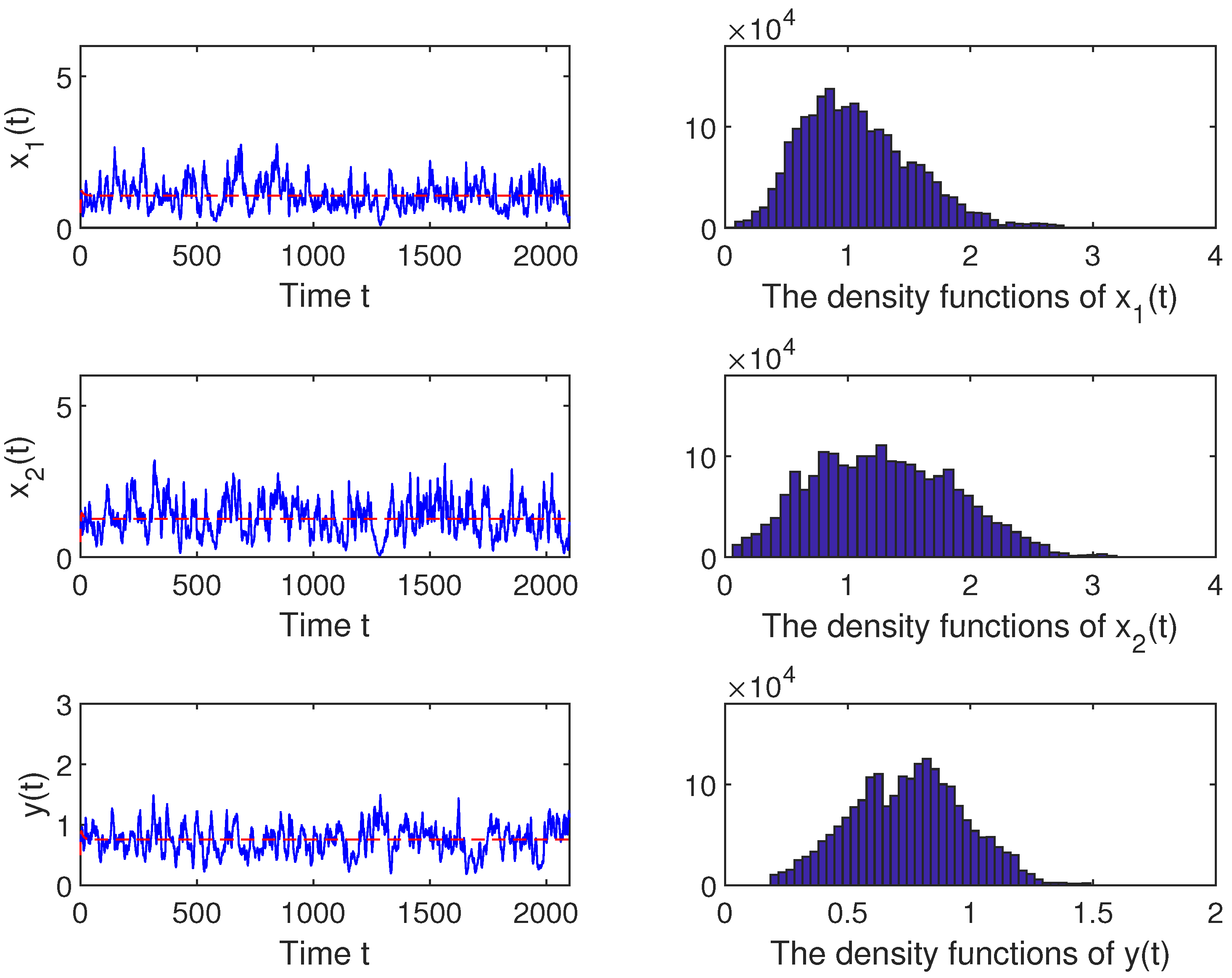
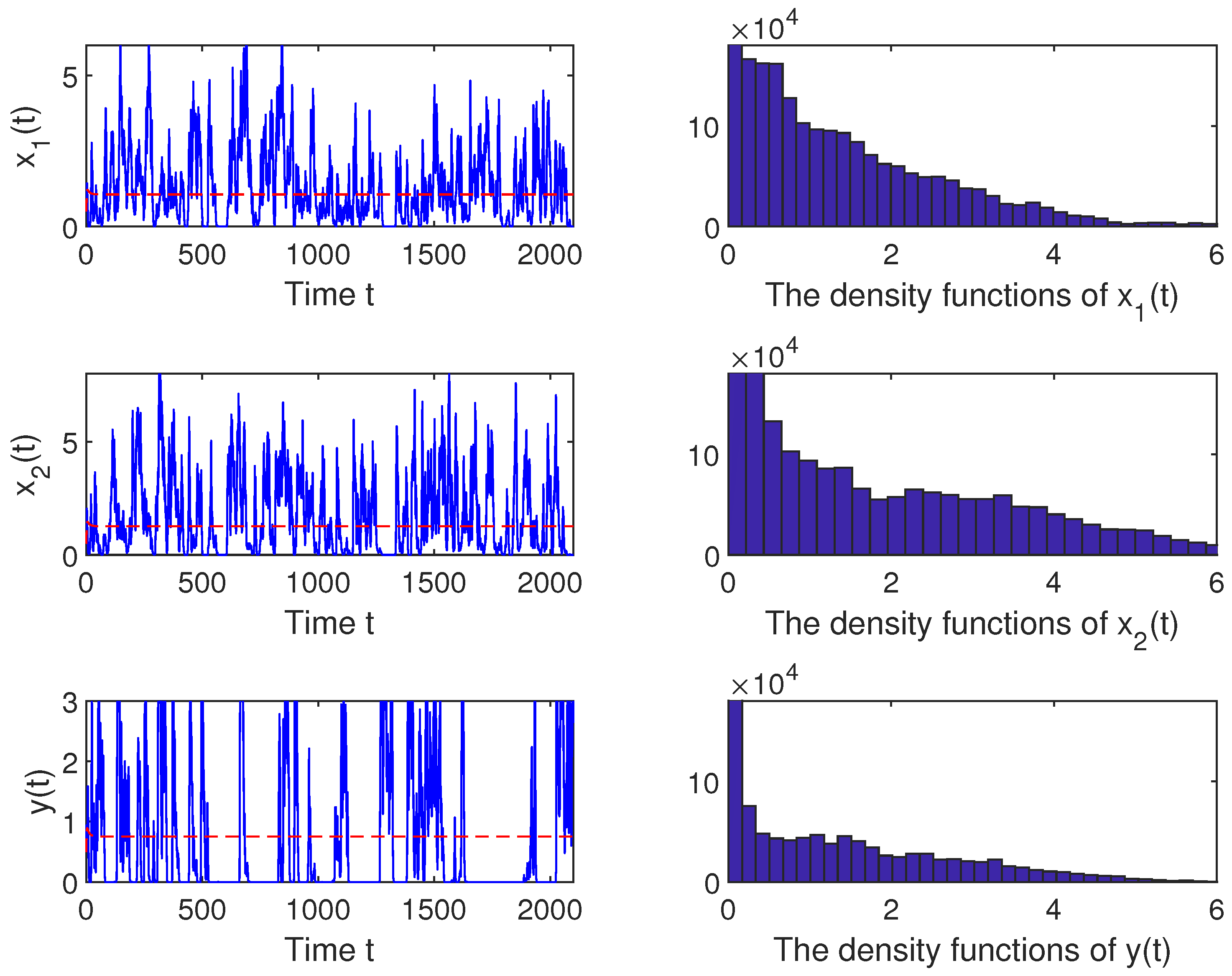
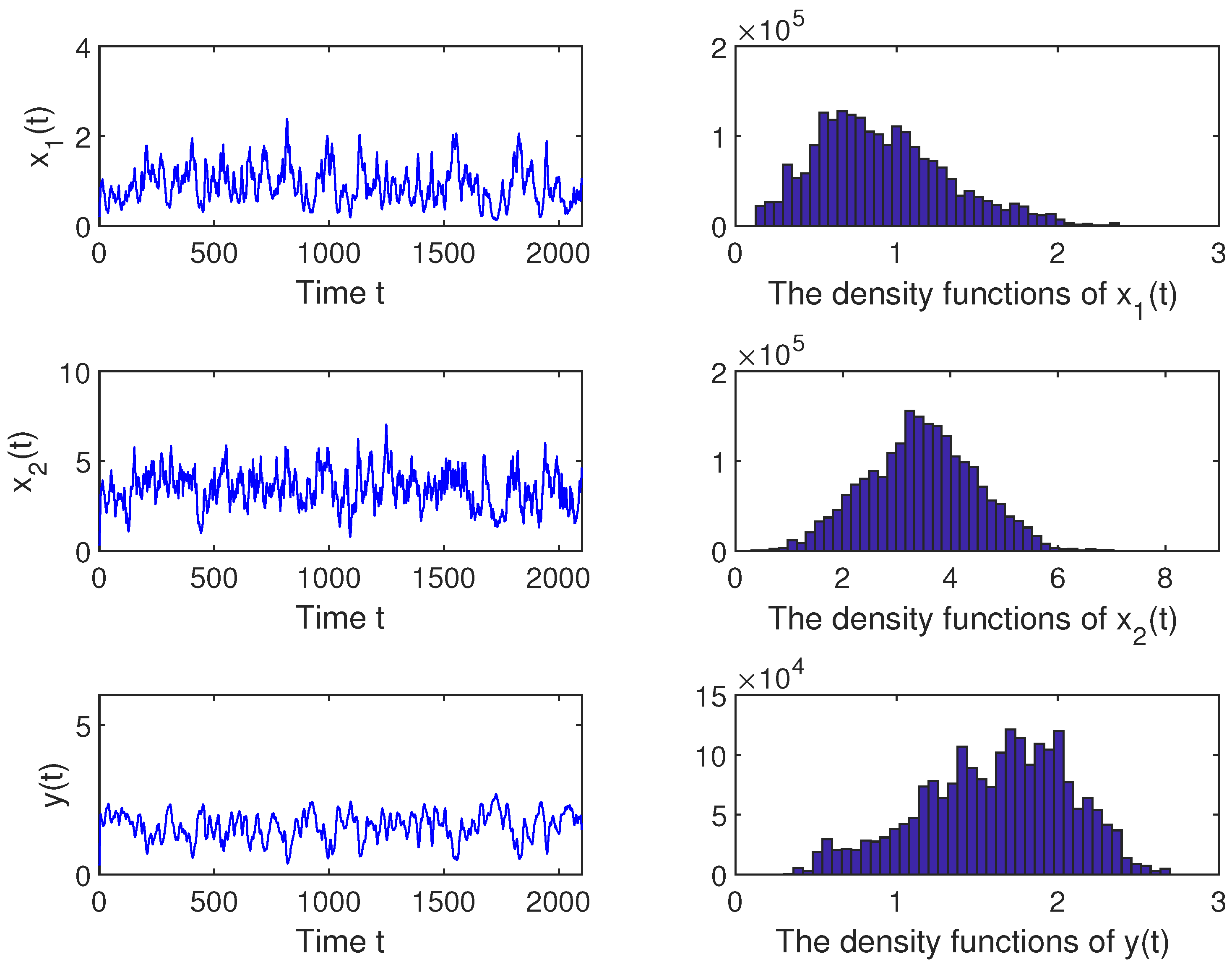
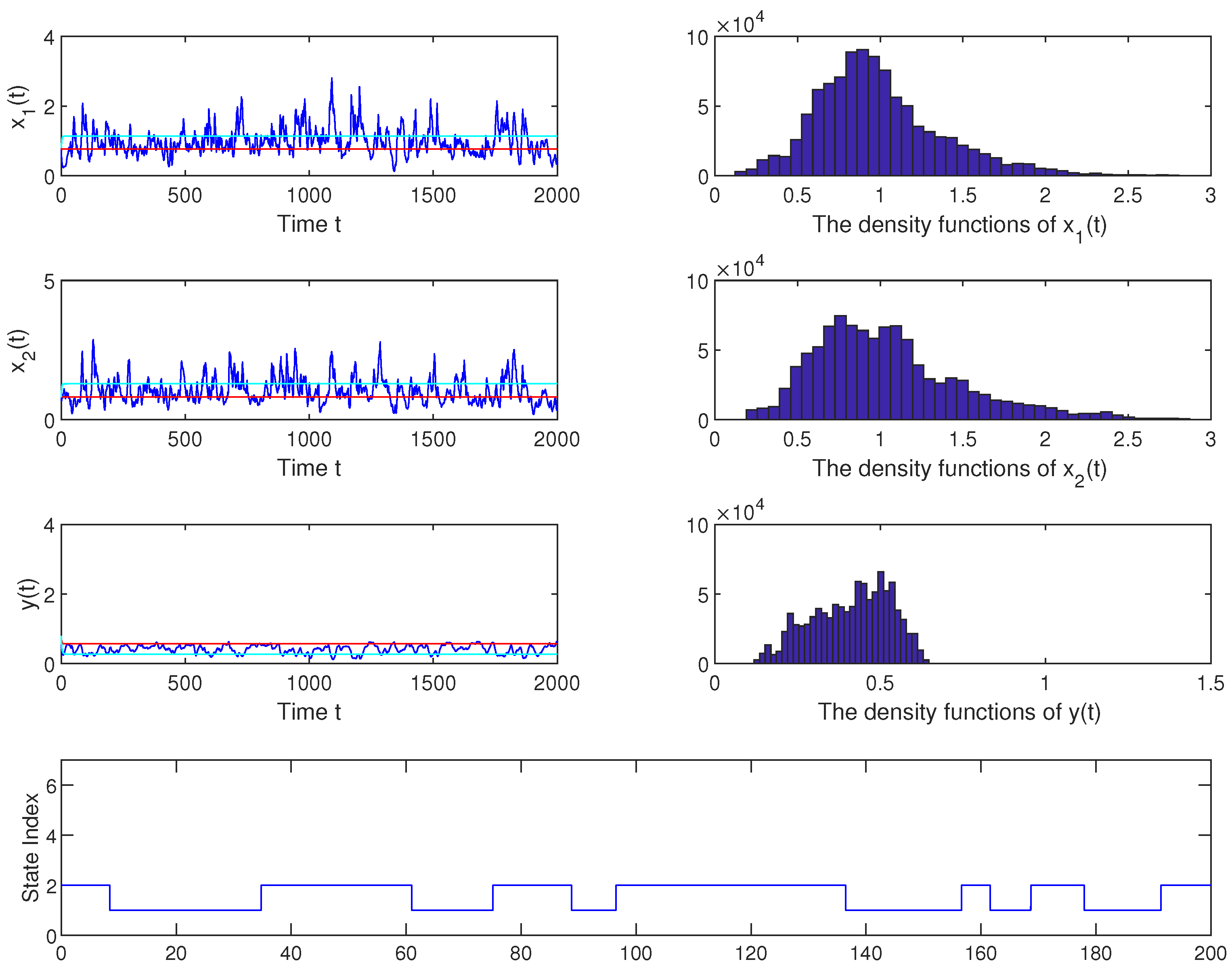
5. Numerical Simulation

Following Higham’s [45] work, we implement the Milstein method in this section to verify the above analytical results.

We perform numerical analysis on model (18) with the OU process, providing simulation-based evidence to verify the analytical conclusions derived in this paper. More specifically, the validation is conducted in four parts: (i) We numerically simulate both scenarios where the prerequisite conditions are satisfied and violated, thereby verifying that the property holds. (ii) Under the assumptions of Theorem 1, we examine whether the numerical results align with the theoretical predictions. (iii) We discover that $95\%$ or more of the solution distribution lie within a neighborhood. (iv) We extend the baseline model (5) by introducing a Markov regime-switching mechanism.

Case 1. We set the parameters $a_1=0.7$, $a_2=0.6$, $a_3=0.15$, $b_1=0.15$, $b_3=0.85$, $D=0.25$, $b=0.1$, ${\rho }_1={\rho }_2={\rho }_3=0.1$, ${\overline{r}}_1={\overline{r}}_2={\overline{r}}_3=0.8$, ${\sigma }_1={\sigma }_2=0.2$ and ${\sigma }_3=0.1$, the condition of $(a_1-{\sigma }_1)(b_3-{\sigma }_3)>a_3{b}_1$ and $a_2>{\sigma }_2$ are satisfied. Then, gain the positive equilibria $E^{*}(x_1^{*},x_2^{*},y^{*})=(0.9936,1.3333,0.7658)$ of model (1) and ${\displaystyle \underset{t\to \infty }{lim\; sup}\frac{1}{t}\mathbb{E}{\int }_0^t[{(x_1(s)-x_1^{*})}^2+{(x_2(s)-x_2^{*})}^2+{(y(s)-y^{*})}^2+{(r_1(s)-{\overline{r}}_1)}^2+{(r_2(s)-{\overline{r}}_2)}^2+{(r_3(s)-{\overline{r}}_3)}^2]}$ ${\displaystyle ds=5e-6}$, ${\displaystyle \frac{{\sigma }_1}{4D{x}_2^{*}{\rho }_1\mathcal{N}}+\frac{{\sigma }_2}{4D{x}_1^{*}{\rho }_2\mathcal{N}}+\frac{b_1{\sigma }_3}{4a_{3}D{x}_2^{*}{\rho }_3\mathcal{N}}=5.8093}$. Thus, according to Theorem 3, it conforms to the property ${\displaystyle \underset{t\to \infty }{lim\; sup}\frac{1}{t}\mathbb{E}{\int }_0^t[{(x_1(s)-x_1^{*})}^2+{(x_2(s)-x_2^{*})}^2+{(y(s)-y^{*})}^2+{(r_1(s)-{\overline{r}}_1)}^2+{(r_2(s)-{\overline{r}}_2)}^2+{(r_3(s)-{\overline{r}}_3)}^2]}$ ${\displaystyle ds\le \frac{{\sigma }_1}{4D{x}_2^{*}{\rho }_1\mathcal{N}}+\frac{{\sigma }_2}{4D{x}_1^{*}{\rho }_2\mathcal{N}}+\frac{b_1{\sigma }_3}{4a_{3}D{x}_2^{*}{\rho }_3\mathcal{N}}}$ as Figure 1.

In Figure 2, we change the noise intensity to ${\sigma }_1=0.6$, ${\sigma }_2=0.7$ and ${\sigma }_3=0.8$, while keeping all other parameters identical to Case 1. Through a calculation, $(a_1-{\sigma }_1)(b_3-{\sigma }_3)=0.0050$ and $a_3{b}_1=0.0225$, which violate the condition of $(a_1-{\sigma }_1)(b_3-{\sigma }_3)>a_3{b}_1$ and $a_2>{\sigma }_2$. We confirm ${\displaystyle \underset{t\to \infty }{lim\; sup}\frac{1}{t}\mathbb{E}{\int }_0^t[{(x_1(s)-x_1^{*})}^2+{(x_2(s)-x_2^{*})}^2+{(y(s)-y^{*})}^2+{(r_1(s)-{\overline{r}}_1)}^2+{(r_2(s)-{\overline{r}}_2)}^2+{(r_3(s)-{\overline{r}}_3)}^2]}$ ${\displaystyle ds=26e-5}$, ${\displaystyle \frac{{\sigma }_1}{4D{x}_2^{*}{\rho }_1\mathcal{N}}+\frac{{\sigma }_2}{4D{x}_1^{*}{\rho }_2\mathcal{N}}+\frac{b_1{\sigma }_3}{4a_{3}D{x}_2^{*}{\rho }_3\mathcal{N}}=-17.4729}$. Therefore, it is inconsistent with the conclusion of Theorem 3.

Case 2. We set the parameters $a_1=0.58$, $a_2=0.21$, $a_3=0.35$, $b_1=0.29$, $b_3=0.3$, $D=0.05$, ${\rho }_1={\rho }_2={\rho }_3=0.1$, ${\overline{r}}_1={\overline{r}}_2={\overline{r}}_3=0.8$, ${\sigma }_1={\sigma }_2=0.1$ and ${\sigma }_3=0.01$. Through a calculation, we gain the positive equilibria $E^{*}(x_1^{*},x_2^{*},y^{*})=(0.8191,3.6252,1.7110)$ of model (5). In view of Theorem 4, the parameter ${\displaystyle \omega =\frac{D^2}{2{\sigma }_1}+\frac{D^2}{2{\sigma }_2}+2D(x_1^{*}+x_2^{*})+\frac{{\sigma }_1}{2{\rho }_1}+\frac{{\sigma }_2}{2{\rho }_2}+\frac{{\sigma }_3}{2{\rho }_3}=1.4348}$ satisfies the criterion that ${\displaystyle \omega <min\left\{\left(a_1-{\sigma }_1+b_1{\sigma }_1+\frac{a_3}{4{\sigma }_3}\right){(x_1^{*})}^2,\left(a_2-{\sigma }_2\right){(x_2^{*})}^2,\right.\left.\left(b_3-\frac{{\sigma }_3}{2}+a_3{\sigma }_3+\frac{b_1}{4{\sigma }_1}\right){(y^{*})}^2\right\}=1.4419}$. Thus, the stochastic model (18) with the OU process has a unique stationary distribution as illustrated in Figure 3.

We choose the same parameters $a_1$, $a_2$, $a_3$, $b_1$, $b_3$, and D as Case 2, then figure a three-dimensional scatter plot of the model (18) distribution. Figure 2 reveals that over $95\%$ of the population is confined to a neighborhood (calculated with the radius $R\le 0.5929$), exhibiting an approximate circular or elliptical geometry centered at $E^{*}(x_1^{*},x_2^{*},y^{*})$ (marked by the red star in Figure 4).

Case 3. Considering the corresponding model (5) with the incorporation of Markov switching [43], we provide the following model.

$$\left\{\begin{array}{c}{\displaystyle d{x}_1(t)=\left\{x_1(t)\left[r_1-a_1{x}_1(t)-\frac{b_{1}y(t)}{1+b{x}_1(t)}\right]+D\left[x_2(t)-x_1(t)\right]\right\}dt,}\hfill \\ {\displaystyle d{x}_2(t)=\left\{x_2(t)\left[r_2-a_2{x}_2(t)\right]+D\left[x_1(t)-x_2(t)\right]\right\}dt,}\hfill \\ {\displaystyle dy(t)=\left\{y(t)\left[r_3-a_3{x}_1(t)-b_{3}y(t)\right]\right\}dt,}\hfill \\ {\displaystyle d{r}_1(t)={\rho }_1[{\overline{r}}_1(r(t))-r_1(t)]dt+{\sigma }_1(r(t))d{W}_1(t),}\hfill \\ {\displaystyle d{r}_2(t)={\rho }_2[{\overline{r}}_2(r(t))-r_2(t)]dt+{\sigma }_2(r(t))d{W}_2(t),}\hfill \\ {\displaystyle d{r}_3(t)={\rho }_3[{\overline{r}}_3(r(t))-r_3(t)]dt+{\sigma }_3(r(t))d{W}_3(t),}\hfill \end{array}\right.$$

(24)

where $r(t)$ represents a continuous-time Markov chain taking values in a finite state space $\mathcal{M}=\left\{1,2,\dots ,N\right\}$ and operating on a probability space. The OU process $r_i$ follows the normal distribution $\mathbb{N}=\left({\sum }_{k\in \mathcal{M}}{\pi }_k{\overline{r}}_i(k),{\sum }_{k\in \mathcal{M}}{\pi }_k\left[{\displaystyle \frac{{\sigma }_i^2(k)}{2{\rho }_i(k)}}+{\left({\overline{r}}_i(k)-{\sum }_{j\in \mathcal{M}}{\pi }_j{\overline{r}}_i(j)\right)}^2\right]\right)$ by calculation when $t\to \infty$ (see [43]).

Then, we set the parameters $a_1=0.7$, $a_2=0.6$, $a_3=0.15$, $b_1=0.15$, $b_3=0.85$, $D=0.25$, $b=0.1$, ${\rho }_1={\rho }_2={\rho }_3=0.1$, ${\overline{r}}_1(1)=0.6$, ${\overline{r}}_2(1)=0.5$, ${\overline{r}}_3(1)=0.6$, ${\sigma }_1(1)=0.1$, ${\sigma }_2(1)=0.1$, ${\sigma }_3(1)=0.01$, ${\overline{r}}_1(2)=0.8$, ${\overline{r}}_2(2)=0.8$, ${\overline{r}}_3(2)=0.4$, ${\sigma }_1(2)=0.2$, ${\sigma }_2(2)=0.2$, ${\sigma }_3(2)=0.03$ and formulate $r(t)$ as a Markov chain in model (5). It is evident that after incorporating the Markov chain, species $x_1$, $x_2$, and y can coexist in Figure 5.

6. Conclusions

In this paper, we study a stochastic competitive Lotka–Volterra model (5) incorporating two species with a Holling Type-II under diffusion and the OU process. The growth and mortality rates are driven by the OU process, and we investigate their effects on population dynamics and ecosystem stability. Next, our analysis demonstrates the existence and uniqueness of the global solution to model (5), as well as the boundedness of moments and the asymptotic behavior of the solution. Moreover, we derive sufficient conditions for the asymptotic stability of the positive equilibrium point by using the Lyapunov function, and we further derive the constant b affecting the property. Additionally, we introduce a transformation and gain the sufficient criteria that guarantee the existence of a stationary distribution for model (18). It is worth mentioning that we generalize Liu’s work, where parameter $b=0$ for model (1.5) in [9]. Finally, we build several numerical simulations of model (18), verifying the existence of a unique stationary distribution. And simulations show that at least $95\%$ of the population is distributed within a circular or elliptical neighborhood centered at $E^{*}(x_1^{*},x_2^{*},y^{*})$ with a non-zero radius. We also implement numerical simulations for a regime-switching competitive ecosystem model combining diffusion and OU processes, hence formulating $r(t)$ in model (5) as a Markov chain. These findings highlight the significant influence of noise intensity and dispersal on the stability and persistence of species in fragmented habitats.

However, several aspects warrant further investigation. Due to the addition of the Holling Type-II functional response to model (5), the complexity has increased. This paper does not theoretically establish the extinction property, nor do the numerical simulations demonstrate a more pronounced extinction effect with increasing noise intensity. In the future, we will continue to study the extinction property. Additionally, since the current asymptotic stability results of the model are only valid in the mean sense, we hope to remove the mean condition and achieve almost surely global asymptotic stability results on the basis of the existing research [46] in the future. At long last, subsequent research can introduce the Black–Karasinski process [39] and spatial factors [12] into model (5), which is more meaningful in actual works.

References

1. Lotka, A.J. Undamped oscillations derived from the law of mass action. J. Am. Chem. Soc. 1920, 42, 1595–1599. [Google Scholar] [CrossRef]
2. Volterra, V. Variazioni e Fluttuazioni del Numero d’Individui in Specie Animali Conviventi; Societá Anonima Tipografica “Leonardo da Vinci”: Rome, Italy, 1927; Volume 2. [Google Scholar]
3. Wu, S.; Wang, Y.; Geng, D. Dynamic and pattern formation of a diffusive predator-prey model with indirect prey-taxis and indirect predator-taxis. Nonlinear Anal. Real World Appl. 2025, 84, 104299. [Google Scholar] [CrossRef]
4. Zhang, J.; Chen, L.; Chen, X.D. Persistence and global stability for two-species nonautonomous competition Lotka-Volterra patch-system with time delay. Nonlinear Anal. Real World Appl. 1999, 37, 1019–1028. [Google Scholar] [CrossRef]
5. Lotka, A.J. Elements of Physical Biology; Williams & Wilkins: Philadelphia, PA, USA, 1925. [Google Scholar]
6. Ji, C.; Jiang, D.; Shi, N. Analysis of a predator-prey model with modified Leslie-Gower and Holling-type II schemes with stochastic perturbation. J. Math. Anal. Appl. 2009, 359, 482–498. [Google Scholar] [CrossRef]
7. Danane, J.; Yavuz, M.; Yıldız, M. Stochastic modeling of three-species Prey-Predator model driven by Lévy Jump with Mixed Holling-II and Beddington-DeAngelis functional responses. Fractal Fract. 2023, 7, 751. [Google Scholar] [CrossRef]
8. Alnafisah, Y.; El-Shahed, M. Deterministic and Stochastic Prey-Predator Model for Three Predators and a Single Prey. Axioms 2022, 11, 156. [Google Scholar] [CrossRef]
9. Liu, Q.; Chen, Q. Asymptotic stability of a stochastic Lotka-Volterra competition model with dispersion and Ornstein-Uhlenbeck process. Appl. Math. Lett. 2024, 157, 109163. [Google Scholar] [CrossRef]
10. Nguyen, D.H.; Yin, G. Coexistence and exclusion of stochastic competitive Lotka-Volterra models. J. Differ. Equ. 2017, 262, 1192–1225. [Google Scholar] [CrossRef]
11. Hening, A.; Nguyen, D.H. Coexistence and extinction for stochastic Kolmogorov systems. Ann. Appl. Probab. 2018, 28, 1893–1942. [Google Scholar] [CrossRef]
12. Su, T.; Kao, Y.; Jiang, D. Dynamical behaviors of a stochastic SIR epidemic model with reaction-diffusion and spatially heterogeneous transmission rate. Chaos Solitons Fractals 2025, 195, 116283. [Google Scholar] [CrossRef]
13. Mohd, M.H.; Murray, R.; Plank, M.J.; Godsoe, W. Effects of dispersal and stochasticity on the presence-absence of multiple species. Ecol. Model. 2016, 342, 49–59. [Google Scholar] [CrossRef]
14. Ji, W.; Zhang, Y.; Liu, M. Dynamical bifurcation and explicit stationary density of a stochastic population model with Allee effects. Appl. Math. Lett. 2021, 111, 106662. [Google Scholar] [CrossRef]
15. Maller, R.A.; Müller, G.; Szimayer, A. Ornstein-Uhlenbeck processes and extensions. In Handbook of Financial Time Series; Springer: Berlin/Heidelberg, Germany, 2009; pp. 421–437. [Google Scholar]
16. Wu, S.; Yuan, S.; Lan, G.; Zhang, T. Understanding the dynamics of hepatitis B transmission: A stochastic model with vaccination and Ornstein-Uhlenbeck process. Appl. Math. Comput. 2024, 476, 128766. [Google Scholar] [CrossRef]
17. Allen, E. Environmental variability and mean-reverting processes. Discrete Contin. Dyn. Syst. Ser. B. 2016, 21, 2073–2089. [Google Scholar] [CrossRef]
18. Zhou, Y.; Jiang, D. Dynamical behavior of a stochastic SIQR epidemic model with Ornstein-Uhlenbeck process and standard incidence rate after dimensionality reduction. Commun. Nonlinear Sci. Numer. Simul. 2023, 116, 106878. [Google Scholar] [CrossRef]
19. Wang, H.; Zuo, W.; Jiang, D. Dynamical analysis of a stochastic epidemic HBV model with log-normal Ornstein-Uhlenbeck process and vertical transmission term. Chaos Solitons Fractals 2023, 177, 114235. [Google Scholar] [CrossRef]
20. Su, X.; Zhang, X.; Jiang, D. Dynamics of a stochastic HBV infection model with general incidence rate, cell-to-cell transmission, immune response and Ornstein-Uhlenbeck process. Chaos Solitons Fractals 2024, 186, 115208. [Google Scholar] [CrossRef]
21. Rudnicki, R.; Pichór, K. Influence of stochastic perturbation on prey-predator systems. Math. Biosci. 2007, 206, 108–119. [Google Scholar] [CrossRef]
22. Mao, X. Stochastic Differential Equations and Applications; Elsevier: Amsterdam, The Netherlands, 2007. [Google Scholar]
23. Mao, X.; Sabanis, S.; Renshaw, E. Asymptotic behaviour of the stochastic Lotka-Volterra model. J. Math. Anal. Appl. 2003, 287, 141–156. [Google Scholar] [CrossRef]
24. Valenti, D.; Giuffrida, A.; Denaro, G.; Pizzolato, N.; Curcio, L.; Mazzola, S.; Basilone, G. Noise induced phenomena in the dynamics of two competing species. Math. Model. Nat. Phenom. 2016, 11, 74. [Google Scholar] [CrossRef]
25. Xia, Y.; Yuan, S. Survival analysis of a stochastic predator-prey model with prey refuge and fear effect. J. Biol. Dyn. 2020, 14, 871–892. [Google Scholar] [CrossRef] [PubMed]
26. Mondal, S.; Samanta, G.P. Impact of fear on a predator-prey system with prey-dependent search rate in deterministic and stochastic environment. Nonlinear Dyn. 2021, 104, 2931–2959. [Google Scholar] [CrossRef]
27. Zhang, Y.; Gao, S.; Chen, S. A stochastic predator-prey eco-epidemiological model with the fear effect. Appl. Math. Lett. 2022, 134, 108300. [Google Scholar] [CrossRef]
28. Mondal, B.; Ghosh, U.; Sarkar, S.; Tiwari, P.K. A generalist predator-prey system with the effects of fear and refuge in deterministic and stochastic environments. Math. Comput. Simul. 2024, 225, 968–991. [Google Scholar] [CrossRef]
29. Liu, M.; Wang, K. Global stability of a nonlinear stochastic predator-prey system with Beddington-DeAngelis functional response. Commun. Nonlinear Sci. Numer. Simul. 2011, 16, 1114–1121. [Google Scholar] [CrossRef]
30. Zhou, B.; Jiang, D.; Hayat, T. Analysis of a stochastic population model with mean-reverting Ornstein-Uhlenbeck process and Allee effects. Commun. Nonlinear Sci. Numer. Simul. 2022, 111, 106450. [Google Scholar] [CrossRef]
31. Rudnicki, R. Long-time behaviour of a stochastic prey-predator model. Stoch. Processes Their Appl. 2003, 108, 93–107. [Google Scholar] [CrossRef]
32. Zhou, B.; Jiang, D.; Han, B.; Hayat, T. Threshold dynamics and density function of a stochastic epidemic model with media coverage and mean-reverting Ornstein-Uhlenbeck process. Math. Comput. Simul. 2022, 196, 15–44. [Google Scholar] [CrossRef]
33. Liu, Q.; Jiang, D. Periodic solution and stationary distribution of stochastic predator-prey models with higher-order perturbation. J. Nonlinear Sci. 2018, 28, 423–442. [Google Scholar] [CrossRef]
34. Yang, Q.; Zhang, X.; Jiang, D. Dynamical behaviors of a stochastic food chain system with Ornstein-Uhlenbeck process. J. Nonlinear Sci. 2022, 32, 34. [Google Scholar] [CrossRef]
35. Ge, J.; Ji, W.; Liu, M. Threshold behavior of a stochastic predator-prey model with fear effect and regime-switching. Appl. Math. Lett. 2025, 164, 109476. [Google Scholar] [CrossRef]
36. Hieu, N.T.; Nguyen, D.H.; Nguyen, N.N.; Yin, G. Analyzing a class of stochastic SIRS models under imperfect vaccination. J. Frankl. Inst. 2024, 361, 1284–1302. [Google Scholar] [CrossRef]
37. Yang, A.; Wang, H.; Yuan, S. Tipping time in a stochastic Leslie predator-prey model. Chaos Solitons Fractals 2023, 171, 113439. [Google Scholar] [CrossRef]
38. Blanchini, F.; Miani, S. A new class of universal Lyapunov functions for the control of uncertain linear systems. IEEE Trans. Autom. Control 2002, 44, 641–647. [Google Scholar] [CrossRef]
39. Han, B.; Jiang, D. Global dynamics of a stochastic smoking epidemic model driven by Black-Karasinski process. Appl. Math. Lett. 2025, 160, 109324. [Google Scholar] [CrossRef]
40. Mu, X.; Jiang, D. Dynamics caused by the mean-reverting Ornstein-Uhlenbeck process in a stochastic predator-prey model with stage structure. Chaos Solitons Fractals 2024, 179, 114445. [Google Scholar] [CrossRef]
41. Roozen, H. An asymptotic solution to a two-dimensional exit problem arising in population dynamics. SIAM J. Appl. Math. 1989, 49, 1793–1810. [Google Scholar] [CrossRef]
42. Ji, C.; Jiang, D. Dynamics of a stochastic density dependent predator-prey system with Beddington-DeAngelis functional response. J. Math. Anal. Appl. 2011, 381, 441–453. [Google Scholar] [CrossRef]
43. Ma, C.; Zhang, X.; Yuan, R. Dynamic analysis of a stochastic regime-switching Lotka-Volterra competitive system with distributed delays and Ornstein-Uhlenbeck process. Chaos Solitons Fractals 2025, 190, 115765. [Google Scholar] [CrossRef]
44. Khasminskii, R. Stochastic Stability of Differential Equations; Springer Science & Business Media: Berlin/Heidelberg, Germany, 2011; Volume 66. [Google Scholar]
45. Higham, D.J. An algorithmic introduction to numerical simulation of stochastic differential equations. SIAM Rev. 2001, 43, 525–546. [Google Scholar] [CrossRef]
46. Li, X.; Liu, Q. Asymptotical stability of a stochastic SIQRS epidemic model with log-normal Ornstein-Uhlenbeck process. Appl. Math. Lett. 2025, 166, 109551. [Google Scholar] [CrossRef]
Figure 1. The solutions of the stochastic model (5) with the OU process and its density function under the parameter conditions in Case 1. The blue lines stand for the solution of model (5), and the red lines represent the solution of deterministic model (1).
Axioms 14 00443 g001
Figure 2. The conditions ( a 1 σ 1 ) ( b 3 σ 3 ) > a 3 b 1 and a 2 > σ 2 are not satisfied.
Axioms 14 00443 g002
Figure 3. The solutions of the stochastic model (18) with the OU process under the parameter conditions in Case 2; the density function diagrams of x 1 ( t ) , x 2 ( t ) and y ( t ) .
Axioms 14 00443 g003
Figure 4. The distribution of the stochastic model (18) around point E * = ( 0.8191 , 3.6252 , 1.7110 ) .
Axioms 14 00443 g004
Figure 5. The solution of model (5) and its density function, where the blue line denotes the stochastic model (5) with regime switching, the red line and cyan line denotes r = 1 and r = 2 in the corresponding determine model, respectively. The last image is the partial state-switching trajectory.
Axioms 14 00443 g005
Disclaimer/Publisher’s Note: The statements, opinions and data contained in all publications are solely those of the individual author(s) and contributor(s) and not of MDPI and/or the editor(s). MDPI and/or the editor(s) disclaim responsibility for any injury to people or property resulting from any ideas, methods, instructions or products referred to in the content.