Copula-Based Bivariate Modified Fréchet–Exponential Distributions: Construction, Properties, and Applications

Abstract

The classical exponential model, despite its flexibility, fails to describe data with non-constant failure or between-event dependency. To overcome this limitation, two new bivariate lifetime distributions are introduced in this paper. The Farlie–Gumbel–Morgenstern (FGM)-based and Ali–Mikhail–Haq (AMH)-based modified Fréchet–exponential (MFE) models, by embedding the flexible MEF margin in the FGM and AMH copulas. The resulting distributions accommodate a wide range of positive or negative dependence while retaining analytical traceability. Closed-form expressions for the joint and marginal density, survival, hazard, and reliability functions are derived, together with product moments and moment-generating functions. Unknown parameters are estimated through the maximum likelihood estimation (MLE) and inference functions for margins (IFM) methods, with asymptotic confidence intervals provided for these parameters. An extensive Monte Carlo simulation quantifies the bias, mean squared error, and interval coverage, indicating that IFM retains efficiency while reducing computational complexity for moderate sample sizes. The models are validated using two real datasets, from the medical sector regarding the infection recurrence times of 30 kidney patients undergoing peritoneal dialysis, and from the economic sector regarding the growth of the gross domestic product (GDP). Overall, the proposed copula-linked MFE distributions provide a powerful and economical framework for survival analysis, reliability, and economic studies.

1. Introduction

The exponential distribution is widely used in applied statistics due to its simplicity and memoryless property, which makes it suitable for modeling the time between independent events. However, in many real-world applications, the failure rate is often not constant. This limitation of the exponential distribution has led to the development of several generalizations, such as the Marshall–Olkin exponential [1], weighted exponential [2], Kumaraswamy Marshall–Olkin exponential [3], and Lomax exponential distributions [4], among others. These models provide greater flexibility in modeling complex datasets, such as those with varying failure rates.

One such generalization is the modified MFE distribution [5], which demonstrates better results in modeling real-world datasets compared to other versions of the exponential distribution. This makes the MFE distribution particularly attractive and relevant for medical and economic applications.

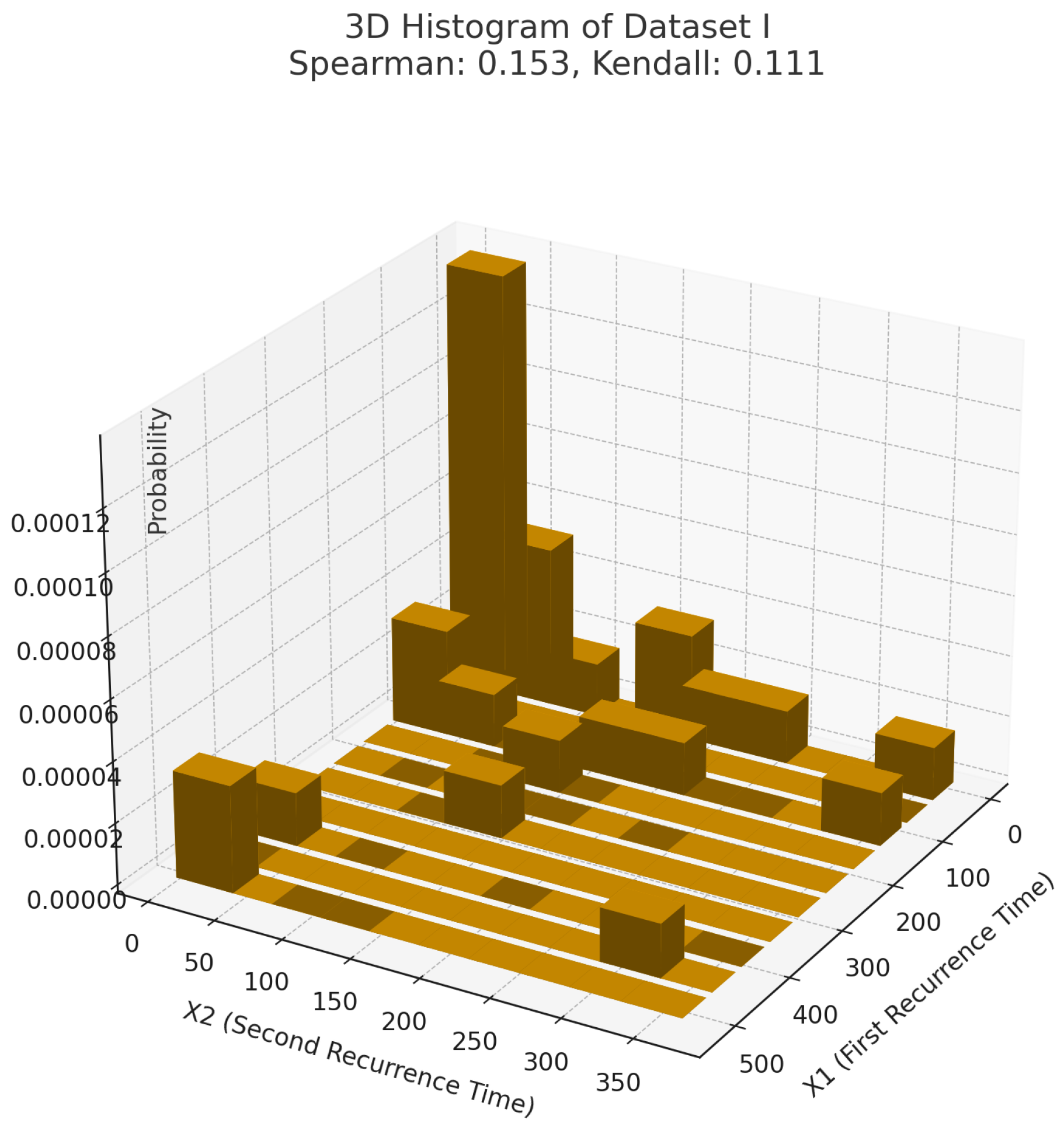
In the context of dialysis patients, infection at the catheter insertion site is a critical complication. Each time an infection occurs, the catheter must be removed, the infection treated, and a new catheter reinserted. This cycle continues throughout the patient’s treatment, making the recurrence times between infections—denoted as $X_1$ (first recurrence time) and $X_2$ (second recurrence time)—a vital measure for predicting future complications and optimizing patient care.

A random variable X is said to follow the MFE distribution with parameters $\lambda$$>0$ as a scale parameter and $\alpha$$>0$ as a shape parameter if the probability density function (pdf) is given by

$$f_{MFED}\left(x\right)={\displaystyle \frac{\alpha \lambda e^{-\lambda x-{\left(1-e^{-\lambda x}\right)}^{\alpha }}{\left(1-e^{-\lambda x}\right)}^{\left(\alpha -1\right)}}{1-e^{-1}}},x>0,$$

(1)

while the cumulative distribution function (cdf) is given by

$$F_{MFED}\left(x\right)={\displaystyle \frac{e^{-{\left(1-e^{-\lambda x}\right)}^{\alpha }}-1}{e^{-1}-1}},x>0.$$

(2)

In recent years, copula-based models have gained significant attention in modeling complex dependence structures across various fields such as finance, hydrology, and reliability engineering (Nelsen [6]; Joe [7]). Among these, the FGM and AMH families have proven particularly valuable due to their flexibility and ease of construction (Durante and Sempi [8]). At the same time, modifications of classical lifetime distributions, such as the Fréchet–exponential distribution, have been proposed to improve model fitting to real-world data.

In this study, we introduce two new copula-based distributions: the FGM-based modified Fréchet–exponential (FGMBMFE) distribution and the AMH-based modified Fréchet–exponential (AMHBMFE) distribution. These models aim to capture a broader range of dependence structures and tail behaviors by integrating copula dependence into the baseline modified Fréchet–exponential distribution. The construction of these models leverages the respective properties of the FGM and AMH copulas, providing flexible yet tractable formulations suitable for various applications.

The main objective of this work is to develop the theoretical properties of the FGMBMFE and AMHBMFE distributions, including their marginal behaviors, joint distributions, and dependence characteristics. To assess the practical performance of the proposed models, several numerical experiments and real-data applications are presented in later sections. These examples are intended to illustrate the estimation techniques, such as the maximum likelihood estimation (MLE) and inference functions for margins (IFM) methods, as well as to evaluate the models’ efficiency and goodness of fit. See, for example, [9,10,11,12,13,14,15,16].

Copulas are functions that combine multivariate distribution functions with uniform $(0,1)$ margins according to Nelsen [6]. An easy way to describe a multivariate distribution with a dependent structure is to use a copula. The n-dimensional copula (C) exists for all $x_1$, …, $x_n$, and if F is continuous, then C is defined only by $F(x_1,\dots ,x_n)=C(F_1\left(x_1\right),\dots ,F_n\left(x_n\right))$. According to Sklar [17], the cdf and pdf copulas for the two random variables $X_1$ and $X_2$, with distribution functions $F_1\left(x_1\right)$ and $F_2\left(x_2\right)$, are as follows:

$$F(x_1,x_2)=C(F_1\left(x_1\right),F_2\left(x_2\right))$$

(3)

and

$$f(x_1,x_2)=f_1\left(x_1\right)f_2\left(x_2\right)c(F_1\left(x_1\right),F_2\left(x_2\right)).$$

(4)

There are many bivariate distributions obtained using copula functions, such as the bivariate generalized exponential distribution using the Clayton copula in [18], the bivariate generalized exponential distribution using the FGM and Plackett copulas in [19], the bivariate Weibull distribution using the FGM copula in [20], and other bivariate distributions using copula functions.

This paper introduces two bivariate models: the FGM-based modified Fréchet–exponential (FGMBMFE) distribution and the AMH-based modified Fréchet–exponential (AMHBMFE) distribution. These models are designed to analyze the recurrence times of infections in kidney patients using portable dialysis machines. By providing enhanced predictions and facilitating improved infection risk management. These models aim to contribute to better patient outcomes. Another application is related to GDP growth.

Table 1. The joint cdf and pdf of the FGM and AMH copulas.

Copula	$C(F_1\left(x_1\right),F_2\left(x_2\right))$	$c(F_1\left(x_1\right),F_2\left(x_2\right))$	$\theta$
FGM	$F_1\left(x_1\right)F_2\left(x_2\right)(1+\theta (1-F_1\left(x_1\right))(1-F_2\left(x_2\right)))$	$1+\theta (1-2F_1\left(x_1\right))(1-2F_2\left(x_2\right))$	$\theta \in \{-1,1\}$
AMH	${\displaystyle \frac{F_1\left(x_1\right)F_2\left(x_2\right)}{1-\theta (1-F_1\left(x_1\right))(1-F_2\left(x_2\right))}}$	${\displaystyle \frac{1-\theta +2\theta \left(\frac{F_1\left(x_1\right)F_2\left(x_2\right)}{1-\theta (1-F_1\left(x_1\right))(1-F_2\left(x_2\right))}\right)}{{(1-\theta (1-F_1\left(x_1\right))(1-F_2\left(x_2\right)))}^2}}$	$\theta \in \{-1,1\}$

presents the joint cdf and pdf for the FGM and AMH copulas.

The FGM copula is one of the well-known parametric copula families. This family was first introduced by Gumbel [21]. The formula for the Kendall’s and Spearman’s correlation coefficients of the FGM copula was derived by Fredricks and Nelsen [22] as follows:

$${\rho }_{Kendall}={\displaystyle \frac{\theta }{3}}\mathrm{and}{\rho }_{Spearman}={\displaystyle \frac{2}{9}}\theta .$$

The AMH copula is also popular like the FGM copula and it was first presented by Ali, Mikhail, and Haq [23]. The formula for the Kendall’s and Spearman’s correlation coefficients of the AMH copula are discussed by Kumar [24] as follows:

(1)

For $\theta \in (-1,1)$, the Kendall’s correlation coefficient is ${\rho }_{Kendall}=1-{\displaystyle \frac{\left({\left(1-\theta \right)}^{2}log\left(1-\theta \right)+\theta \right)}{3{\theta }^2}}$, or approximately $[0,{\displaystyle \frac{1}{3}}]$.

(2)

For $\theta \in \{-1,1\}$, the Spearman’s correlation coefficient is ${\rho }_{Spearman}$ = $[33-48log2,4{\pi }^2-39]$, or approximately $[-0.2711,0.4784]$.

This study derives important reliability functions, hazard functions, and product moments for the bivariate modified Fréchet–exponential distribution based on the FGM and AMH copulas. We also obtain the moment-generating function for these models, providing additional insights into their properties. Furthermore, we estimate the unknown parameters of both the FGM- and AMH-based models using two estimation methods: Maximum likelihood estimation (MLE) and inference functions for matrices (IFM). The asymptotic confidence intervals for the model parameters are also computed to evaluate the precision of these estimates.

This research aims to explore the usefulness of the modified Fréchet–exponential distribution, in conjunction with the FGM and AMH copulas, for modeling the infection recurrence times of kidney patients using portable dialysis machines, and also for modeling GDP growth with exports of goods and services. The proposed model provides insights into the temporal dynamics of infection recurrence, which can assist medical professionals in anticipating infection risks and optimizing treatment protocols. Additionally, this approach contributes to the growing body of literature on the application of bivariate statistical models in medical case studies, offering a new perspective on handling recurrence data in healthcare settings.

This paper is organized as follows: we present the two bivariate modified Fréchet–exponential distributions based on the FGM and AMH copulas in Section 2. Section 3 discusses some statistical features of the bivariate copula distribution, while Section 4 outlines the parameter estimation methods for the proposed models. The asymptotic confidence intervals are introduced in Section 5. A simulation study in Section 6 compares the efficiency of the models and estimation methods. Section 7 presents the application of real-world data related to the medical and economic fields. Finally, Section 8 concludes with remarks on the utility of the proposed models for data analysis.

2. Bivariate Modified Fréchet–Exponential Distribution

Using Sklar’s theorem [17], we obtain the joint cdf and pdf of the BMFE distribution for any copula using Equations (3) and (4) in addition to the cdf and the pdf of the MFE model.

$$F(x_1,x_2)=C({\displaystyle \frac{e^{-{\Delta }_1^{{\alpha }_1}}-1}{e^{-1}-1}},{\displaystyle \frac{e^{-{\Delta }_2^{{\alpha }_2}}-1}{e^{-1}-1}}),$$

(5)

$$\begin{array}{cc}\hfill f(x_1,x_2)& ={\alpha }_1{\lambda }_1{\left(1-e^{-1}\right)}^{-2}{e}^{-{\lambda }_1{x}_1-{\Delta }_1^{{\alpha }_1}}{\Delta }_1^{\left({\alpha }_1-1\right)}{\alpha }_2{\lambda }_2{e}^{-{\lambda }_2{x}_2-{\Delta }_2^{{\alpha }_2}}{\Delta }_2^{\left({\alpha }_2-1\right)}c({\displaystyle \frac{e^{-{\Delta }_1^{{\alpha }_1}}-1}{e^{-1}-1}},{\displaystyle \frac{e^{-{\Delta }_2^{{\alpha }_2}}-1}{e^{-1}-1}}),\hfill \end{array}$$

(6)

where ${\Delta }_i=1-e^{-{\lambda }_i{x}_i}$. Equations (5) and (6) are utilized to create two BMFE distributions based on the FGM and AMH copulas in the following subsections.

2.1. Survival Functions and Joint Survival Structure

The marginal survival function of the MFE distribution is given by

$$R_i\left(x_i\right)=1-F_{MFED}\left(x_i\right)={\displaystyle \frac{e^{-1}-e^{-{\Delta }_i^{{\alpha }_i}}}{e^{-1}-1}},\mathrm{where}{\Delta }_i=1-e^{-{\lambda }_i{x}_i},i=1,2.$$

Using Sklar’s theorem in the survival domain, the joint survival function of the bivariate model is given by

$$R(x_1,x_2)=Pr(X_1>x_1,X_2>x_2)=\overline{C}(R_1\left(x_1\right),R_2\left(x_2\right)),$$

where $\overline{C}$ is the survival copula defined by

$$\overline{C}(u,v)=u+v-1+C(1-u,1-v).$$

Joint Survival Function for FGM Copula

The survival copula corresponding to the FGM copula is

$${\overline{C}}_{FGM}(u,v)=uv\left[1+\theta (1-u)(1-v)\right],\theta \in [-1,1].$$

Hence, the joint survival function of the FGM-based bivariate MFE distribution model becomes

$$R_{FGM}(x_1,x_2)=R_1\left(x_1\right)R_2\left(x_2\right)\left[1+\theta (1-R_1\left(x_1\right))(1-R_2\left(x_2\right))\right].$$

This expression provides a mathematically rigorous and practically useful formulation for analyzing joint reliability in the presence of dependence between marginal lifetimes. A similar approach may be used to derive the joint survival function using the AMH copula.

2.2. FGM Bivariate Modified Fréchet–Exponential (FGMBMFE) Distribution

Applying the FGM copula transformation described in Table 1, we obtain the following cdf and pdf functions for the FGMBMFE distribution:

$$F(x_1,x_2)={\left(e^{-1}-1\right)}^{-2}\left(e^{-{\Delta }_1^{{\alpha }_1}}-1\right)\left(e^{-{\Delta }_2^{{\alpha }_2}}-1\right)\left(1+\theta \left({\displaystyle \frac{e^{-1}-e^{-{\Delta }_1^{{\alpha }_1}}}{e^{-1}-1}}\right)\left({\displaystyle \frac{e^{-1}-e^{-{\Delta }_2^{{\alpha }_2}}}{e^{-1}-1}}\right)\right)$$

and

$$\begin{array}{cc}\hfill f(x_1,x_2)& ={\displaystyle \frac{{\alpha }_1{\lambda }_1{\alpha }_2{\lambda }_2}{{(1-e^{-1})}^2}}·e^{-{\lambda }_1{x}_1-{\Delta }_1^{{\alpha }_1}}·{\Delta }_1^{{\alpha }_1-1}·e^{-{\lambda }_2{x}_2-{\Delta }_2^{{\alpha }_2}}·{\Delta }_2^{{\alpha }_2-1}\hfill \\ \hfill & ·\left[1+\theta \left(1-2·{\displaystyle \frac{e^{-{\Delta }_1^{{\alpha }_1}}-1}{e^{-1}-1}}\right)\left(1-2·{\displaystyle \frac{e^{-{\Delta }_2^{{\alpha }_2}}-1}{e^{-1}-1}}\right)\right],\hfill \end{array}$$

(7)

respectively, where $x_1,x_2>0$ and ${\alpha }_1,{\lambda }_1,{\alpha }_2,{\lambda }_2>0,-1<\theta <1.$

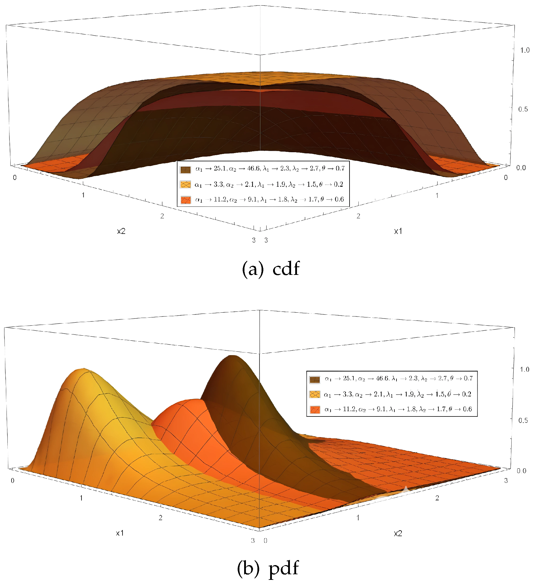
Figure 1 displays the behavior of the FGMBMFE distribution by presenting the cdf and pdf plots for different combinations of the parameters ${\alpha }_1,{\lambda }_1,{\alpha }_2,$ ${\lambda }_2$, and $\theta$, showing the adaptability of the joint cdf and pdf in modeling bivariate skewed data. The graphs were generated using Mathematica 11 by evaluating the closed-form expressions derived in this section. These 3D plots highlight the influence of the parameters on the distribution’s shape and tail behavior.

The joint pdf and cdf of the FGMBMFE distribution displays various shapes depending on the values of its parameters, indicating the joint pdf’s capacity to simulate bivariate skewed data. Although the mathematical properties of the FGMBMFE distributions have been established, it is important to highlight their practical significance. The flexibility introduced through the FGM copula allows the model to capture weak to moderate dependence structures between variables, which are often encountered in reliability engineering and environmental studies. Moreover, the modified Fréchet–exponential marginals enable better modeling of skewed and heavy-tailed data, which cannot be adequately captured by classical exponential or normal models. Therefore, the FGMBMFE distribution provides a useful tool for practitioners seeking models that combine flexibility in marginal behavior with explicit control over dependence, making it valuable for real-world applications where such features are observed.

2.3. AMH Bivariate Modified Fréchet–Exponential (AMHBMFE) Distribution

Applying the AMH copula transformation described in Table 1 with Equations (5) and (6), we obtain the following cdf and pdf for the AMHBMFE distribution:

$$F(x_1,x_2)={\displaystyle \frac{\left(e^{-{\Delta }_1^{{\alpha }_1}}-1\right)\left(e^{-{\Delta }_2^{{\alpha }_2}}-1\right)}{{(e^{-1}-1)}^{-2}-\theta \left(\left(e^{-1}-e^{-{\Delta }_1^{{\alpha }_1}}\right)\left(e^{-1}-e^{-{\Delta }_2^{{\alpha }_2}}\right)\right)}}$$

(8)

and

$$\begin{array}{cc}\hfill f(x_1,x_2)& ={\alpha }_1{\lambda }_1{e}^{-{\lambda }_1{x}_1-{\Delta }_1^{{\alpha }_1}}{\left(1-e^{-1}\right)}^{-2}{\Delta }_1^{\left({\alpha }_1-1\right)}{\alpha }_2{\lambda }_2{e}^{-{\lambda }_2{x}_2-{\Delta }_2^{{\alpha }_2}}{\Delta }_2^{\left({\alpha }_2-1\right)}\hfill \\ \hfill & \left(1-\theta +{\displaystyle \frac{2\theta \left(e^{-{\Delta }_1^{{\alpha }_1}}-1\right)\left(e^{-{\Delta }_2^{{\alpha }_2}}-1\right)}{{(e^{-1}-1)}^{-2}-\theta \left(e^{-1}-e^{-{\Delta }_1^{{\alpha }_1}}\right)\left(e^{-1}-e^{-{\Delta }_2^{{\alpha }_2}}\right)}}\right)\times \hfill \\ \hfill & {\left(1-\theta \left({\displaystyle \frac{e^{-1}-e^{-{\Delta }_1^{{\alpha }_1}}}{e^{-1}-1}}\right)\left({\displaystyle \frac{e^{-1}-e^{-{\Delta }_2^{{\alpha }_2}}}{e^{-1}-1}}\right)\right)}^{-2},\hfill \end{array}$$

(9)

respectively, with $x_1,x_2>0$, ${\alpha }_1,{\lambda }_1,{\alpha }_2,{\lambda }_2>0,\mathrm{and}-1<\theta <1.$

Figure 2 displays the behavior of the AMHBMFE distribution by presenting the cdf and pdf plots for different combinations of the parameters ${\alpha }_1,{\lambda }_1,{\alpha }_2,$ ${\lambda }_2$, and $\theta$, showing the adaptability of the joint cdf and pdf in modeling bivariate skewed data. The graphs were generated using Mathematica 11 by evaluating the closed-form expressions derived in this section. These 3D plots highlight the influence of the parameters on the distribution’s shape and tail behavior.

In addition, the properties of the AMHBMFE distribution offer significant practical advantages. The use of the AMH copula introduces greater flexibility in capturing a wider range of dependence structures, including both positive and negative associations between variables. This flexibility makes the AMHBMFE distribution particularly suitable for modeling real-world datasets where complex, nonlinear dependence patterns are present. Furthermore, modified Fréchet–exponential marginals retain their ability to model skewed and heavy-tailed data, improving the applicability of the distribution to fields such as finance, environmental science, and engineering. Consequently, the AMHBMFE distribution serves as a robust alternative to classical bivariate models, offering both improved marginal behavior and a more adaptable dependence structure.

Since the derivations and properties of the FGMBMFE distribution have been thoroughly presented, and noting the structural similarity between the FGMBMFE and AMHBMFE distributions, which differ mainly in the choice of the copula function (FGM versus AMH), it is deemed sufficient to infer the corresponding properties of the AMHBMFE distribution by analogy. The underlying marginal distributions remain the same, and the main distinction lies in the dependence structure modeled by the AMH copula, which offers greater flexibility. Therefore, detailed derivations for the AMHBMFE distribution are omitted for brevity, without loss of generality.

3. Properties of FGMBMFE Distribution

In this section, we discuss some of the most important statistical properties of the FGMBMFE distribution, including marginal distributions, generating random variables, product moments, and moment-generating and reliability functions.

3.1. Marginal Distributions

The marginal distributions are obtained by modifying the classical Fréchet–exponential distribution to enhance its flexibility and adapt it to a broader range of data characteristics. Specifically, adjustments are made to the original distribution’s scale and shape parameters to allow for greater control over skewness and tail behavior. These modified marginals are then used as the foundational components in the construction of the proposed joint models, wherein the dependence structure between variables is captured using the FGM and AMH copulas, respectively. This approach ensures that both the marginal properties and the dependence behavior are accurately modeled, providing a comprehensive and robust framework for analyzing complex data.

The marginal density functions for $X_1$ and $X_2$, respectively, are

$$f(x_1;{\alpha }_1,{\lambda }_1)={\displaystyle \frac{{\alpha }_1{\lambda }_1{e}^{-{\lambda }_1{x}_1-{\Delta }_1^{{\alpha }_1}}{\Delta }_1^{\left({\alpha }_1-1\right)}}{1-e^{-1}}},x_1>0,{\alpha }_1,{\lambda }_1>0$$

(10)

and

$$f(x_2;{\alpha }_2,{\lambda }_2)={\displaystyle \frac{{\alpha }_2{\lambda }_2{e}^{-{\lambda }_2{x}_2-{\Delta }_2^{{\alpha }_2}}{\Delta }_2^{\left({\alpha }_2-1\right)}}{1-e^{-1}}},x_2>0,{\alpha }_2,{\lambda }_2>0,$$

(11)

which are the modified Fréchet–exponential distribution as shown in Equation (1).

3.2. Generating Random Variables

Nelsen [6] discussed how to generate a sample from a given joint distribution. When using the conditional distribution method, the joint distribution function is as follows:

$$f(x_1,x_2)=f\left(x_1\right)f\left(x_2\right|x_1).$$

The following steps generate a bivariate sample using the conditional technique:

• Generate U and V independently from a uniform $(0,1)$ distribution.
• Set $X_1={\lambda }_1{[-ln(1-U)]}^{{\alpha }_1}.$
• Set $F\left(x_2\right|x_1)=V$ to find $X_2$ by numerical simulation.
• Repeat steps 1–3, n times to obtain $(x_{1i},x_{2i}),i=1,2,\dots ,n.$

3.3. Moment-Generating Function

If the random variable $\left(X_1,X_2\right)$ is distributed as FGMMFE, then the moment-generating function of $\left(X_1,X_2\right)$ is given by

$$\begin{array}{cc}\hfill M_{x_1,x_2}(t_1,t_2)& =E\left(e^{t_1{x}_1}{e}^{t_2{x}_2}\right)={\int }_0^{\infty }{\int }_0^{\infty }{e}^{t_1{x}_1}{e}^{t_2{x}_2}f(x_1,x_2)d{x}_{1}d{x}_2\hfill \\ \hfill & =m_1{m}_2(1+\theta )+{\displaystyle \frac{4\theta }{{\left(e^{-1}-1\right)}^2}}(m_{11}{m}_{22}-m_{11}{m}_2-m_1{m}_{22}+m_1{m}_2)\hfill \\ \hfill & +{\displaystyle \frac{2\theta }{e^{-1}-1}}(-m_{11}{m}_2+m_1{m}_2-m_1{m}_{22}+m_1{m}_2),\hfill \end{array}$$

(12)

where

$$m_1=\sum _{n_1=0}^{\infty }\sum _{m_1=0}^{\infty }\left({\displaystyle \genfrac{}{}{0pt}{}{\left(n_1+1\right){\alpha }_1-1}{m_1}}\right){\displaystyle \frac{{(-1)}^{n_1+m_1}{\alpha }_1}{n_1!\left(1-e^{-1}\right){\lambda }_1}}{\displaystyle \frac{1}{(m_1+1)\left(1-\frac{t}{(m_1+1){\lambda }_1}\right)}}.$$

$$m_2=\sum _{n_2=0}^{\infty }\sum _{m_2=0}^{\infty }\left({\displaystyle \genfrac{}{}{0pt}{}{\left(n_2+1\right){\alpha }_2-1}{m_2}}\right){\displaystyle \frac{{(-1)}^{n_2+m_2}{\alpha }_2}{n_2!\left(1-e^{-1}\right){\lambda }_2}}{\displaystyle \frac{1}{(m_2+1)\left(1-\frac{t}{(m_2+1){\lambda }_2}\right)}}.$$

$$m_{11}=\sum _{n_1=0}^{\infty }\sum _{k_1=0}^{\infty }\sum _{m_1=0}^{\infty }\left({\displaystyle \genfrac{}{}{0pt}{}{\left(n_1+1\right){\alpha }_1+k_1-1}{m_1}}\right){\displaystyle \frac{{(-1)}^{n_1+k_1+m_1}{\alpha }_1}{n_1!k_1!\left(1-e^{-1}\right){\lambda }_1}}{\displaystyle \frac{1}{(m_1+1)\left(1-\frac{t}{(m_1+1){\lambda }_1}\right)}}.$$

and

$$m_{22}=\sum _{n_2=0}^{\infty }\sum _{k_2=0}^{\infty }\sum _{m_2=0}^{\infty }\left({\displaystyle \genfrac{}{}{0pt}{}{\left(n_2+1\right){\alpha }_2+k_2-1}{m_2}}\right){\displaystyle \frac{{(-1)}^{n_2+k_2+m_2}{\alpha }_2}{n_2!k_2!\left(1-e^{-1}\right){\lambda }_2}}{\displaystyle \frac{1}{(m_2+1)\left(1-\frac{t}{(m_2+1){\lambda }_2}\right)}}.$$

It must be clarified that the above series converges under the condition that $t<{\lambda }_1$ and $t<{\lambda }_2$.

3.4. Product Moments

If the random variable $\left(X_1,X_2\right)$ is distributed as FGMMFE, then its rth and sth moments around zero can be expressed as follows:

$$\begin{array}{cc}\hfill {\mu }_{rs}^{\prime }& =E\left(X_1^r{X}_2^s\right)={\int }_0^{\infty }{\int }_0^{\infty }{x}^r{x}^{s}f(x_1,x_2)d{x}_{1}d{x}_2\hfill \\ \hfill & ={\mu }_1{\mu }_2(1+\theta )+{\displaystyle \frac{4\theta }{{\left(e^{-1}-1\right)}^2}}({\mu }_{11}{\mu }_{22}-{\mu }_{11}{\mu }_2-{\mu }_1{\mu }_{22}+{\mu }_1{\mu }_2)\hfill \\ \hfill & +{\displaystyle \frac{2\theta }{e^{-1}-1}}(-{\mu }_{11}{\mu }_2+{\mu }_1{\mu }_2-{\mu }_1{\mu }_{22}+{\mu }_1{\mu }_2),\hfill \end{array}$$

(13)

where ${\mu }_1={\sum }_{n_1=0}^{\infty }{\sum }_{m_1=0}^{\infty }\left(\begin{array}{c}\left(n_1+1\right){\alpha }_1-1\\ m_1\end{array}\right){\displaystyle \frac{{(-1)}^{n_1+m_1}{\alpha }_1}{n_1!\left(1-e^{-1}\right){(m_1+1)}^{r+1}{\lambda }_1^r}}\Gamma (r+1),$

${\mu }_2={\sum }_{n_2=0}^{\infty }{\sum }_{m_2=0}^{\infty }\left(\begin{array}{c}\left(n_2+1\right){\alpha }_2-1\\ m_2\end{array}\right){\displaystyle \frac{{(-1)}^{n_2+m_2}{\alpha }_2}{n_2!\left(1-e^{-1}\right){(m_2+1)}^{s+1}{\lambda }_2^s}}\Gamma (s+1),$

${\mu }_{11}={\sum }_{n_1=0}^{\infty }{\sum }_{k_1=0}^{\infty }{\sum }_{m_1=0}^{\infty }\left(\begin{array}{c}\left(n_1+1\right){\alpha }_1+k_1-1\\ m_1\end{array}\right){\displaystyle \frac{{(-1)}^{n_1+k_1+m_1}{\alpha }_1}{n_1!k_1!\left(1-e^{-1}\right){(m_1+1)}^{r+1}{\lambda }_1^r}}\Gamma (r+1)$ and

${\mu }_{22}={\sum }_{n_2=0}^{\infty }{\sum }_{k_2=0}^{\infty }{\sum }_{m_2=0}^{\infty }\left(\begin{array}{c}\left(n_2+1\right){\alpha }_2+k_2-1\\ m_2\end{array}\right){\displaystyle \frac{{(-1)}^{n_2+k_1+m_2}{\alpha }_2}{n_1!k_1!\left(1-e^{-1}\right){(m_2+1)}^{s+1}{\lambda }_2^s}}\Gamma (s+1).$

These series converge for positive parameter values that are already achieved.

3.5. Reliability Function

According to Osmetti and Chiodini [25], using the reliability function it is easier to describe a joint survival function as a copula of its marginal survival functions, where $X_1$ and $X_2$ are random variables with survival functions $R\left(x_1\right)$ and $R\left(x_2\right)$. The reliability function of the marginal distributions is defined as $R(x_j;{\alpha }_j,{\lambda }_j)=1-F(x_j;{\alpha }_j,{\lambda }_j)={\displaystyle \frac{e^{-1}-e^{-{\left(1-e^{-{\lambda }_j{x}_j}\right)}^{{\alpha }_j}}}{e^{-1}-1}};x>0,{\alpha }_j,{\lambda }_j>0,j=1,2.$

The expression of the joint survival function with copula is defined as follows:

$$R(x_1,x_2)=C(R\left(x_1\right),R\left(x_2\right)),$$

hence, the reliability function of the FGMBMFE distribution is

$$\begin{array}{cc}\hfill R(x_1,x_2)& ={\left(e^{-1}-1\right)}^{-2}(e^{-1}-e^{-{\Delta }_1^{{\alpha }_1}})(e^{-1}-e^{-{\Delta }_2^{{\alpha }_2}})\left(1+\theta \left({\displaystyle \frac{e^{-{\Delta }_1^{{\alpha }_1}}-1}{e^{-1}-1}}\right)\left({\displaystyle \frac{e^{-{\Delta }_2^{{\alpha }_2}}-1}{e^{-1}-1}}\right)\right).\hfill \end{array}$$

(14)

For the first time, Basu [26] defined the bivariate hazard rate function as

$$h(x_1,x_2)={\displaystyle \frac{f(x_1,x_2)}{R(x_1,x_2)}},$$

then, the hazard rate function of FGMBW distribution is written as

$$\begin{array}{cc}\hfill h(x_1,x_2)& ={\displaystyle \frac{{\alpha }_1{\lambda }_1{\alpha }_2{\lambda }_2{e}^{-{\lambda }_1{x}_1-{\Delta }_1^{{\alpha }_1}}}{(e^{-1}-e^{-{\Delta }_1^{{\alpha }_1}})(e^{-1}-e^{-{\Delta }_2^{{\alpha }_2}})}}\times {\displaystyle \frac{{\Delta }_1^{\left({\alpha }_1-1\right)}{e}^{-{\lambda }_2{x}_2-{\Delta }_2^{{\alpha }_2}}{\Delta }_2^{\left({\alpha }_2-1\right)}}{\left(1+\theta \left(\frac{e^{-{\Delta }_1^{{\alpha }_1}}-1}{e^{-1}-1}\right)\left(\frac{e^{-{\Delta }_2^{{\alpha }_2}}-1}{e^{-1}-1}\right)\right)}}\hfill \\ \hfill & \left[1+\theta \left(1-2\times {\displaystyle \frac{e^{-{\Delta }_1^{{\alpha }_1}}-1}{e^{-1}-1}}\right)\left(1-2\times {\displaystyle \frac{e^{-{\Delta }_2^{{\alpha }_2}}-1}{e^{-1}-1}}\right)\right].\hfill \end{array}$$

(15)

4. Parameter Estimation

This section introduces two estimation techniques, the maximum likelihood estimation (MLE) and the inference functions for margins (IFM), which are utilized to estimate the unknown parameters of the FGMBMFE and AMHBMFE distributions; see [27,28] for more details on these techniques.

4.1. Maximum Likelihood Estimation

The maximum likelihood estimator is a one-step parametric approach used to estimate all model parameters together. The log-likelihood function based on copulas is displayed as

$$logL=\sum _{j=1}^n\left[log\left(f_1\left(x_{1j}\right)f_2\left(x_{2j}\right)c(F_1\left(x_{1j}\right),F_2\left(x_{2j}\right);\theta )\right)\right].$$

(16)

Assume ${\Delta }_{1i}=1-e^{-{\lambda }_1{x}_{1i}}$ and ${\Delta }_{2i}=1-e^{-{\lambda }_2{x}_{2i}}$, then the log-likelihood functions of the FGMBMFE and AMHBMEFE distributions are given by

$$\begin{array}{cc}\hfill LogL& =nlog\left({\alpha }_1{\alpha }_2{\lambda }_1{\lambda }_2\right)-2nlog(1-e^{-1})-\sum _{i=1}^n{\lambda }_1{x}_{1i}-\sum _{i=1}^n{\Delta }_{1i}^{{\alpha }_1}-\sum _{i=1}^n{\lambda }_2{x}_{2i}-\sum _{i=1}^n{\Delta }_{2i}^{{\alpha }_2}\hfill \\ \hfill & +\left({\alpha }_1-1\right)\sum _{i=1}^{n}log{\Delta }_{1i}+\left({\alpha }_2-1\right)\sum _{i=1}^{n}log{\Delta }_{2i}+\sum _{i=1}^{n}log\left(c({\displaystyle \frac{e^{-{\Delta }_1^{{\alpha }_1}}-1}{e^{-1}-1}},{\displaystyle \frac{e^{-{\Delta }_2^{{\alpha }_2}}-1}{e^{-1}-1}})\right).\hfill \end{array}$$

(17)

By differentiating the log-likelihood function in Equation (17) when considering each parameter separately, the estimates of all the FGMBMFE parameters are derived as follows:

$$\begin{array}{cc}\hfill {\displaystyle \frac{\partial logL}{\partial {\alpha }_1}}& ={\displaystyle \frac{n}{{\alpha }_1}}-\sum _{i=1}^n{\Delta }_{1i}^{{\alpha }_1}log{\Delta }_{1i}+\sum _{i=1}^{n}log{\Delta }_{1i}+\sum _{i=1}^n{\displaystyle \frac{2{\left(e^{-1}-1\right)}^{-1}\theta \left(a(x_{2i};{\lambda }_2,{\alpha }_2)\right)e^{-{\Delta }_{1i}^{{\alpha }_1}}{\Delta }_{1i}^{{\alpha }_1}log{\Delta }_{1i}}{(1+\theta \left(a(x_{1i};{\lambda }_1,{\alpha }_1)\right)\left(a(x_{2i};{\lambda }_2,{\alpha }_2)\right))}},\hfill \end{array}$$

$$\begin{array}{cc}\hfill {\displaystyle \frac{\partial logL}{\partial {\alpha }_2}}& ={\displaystyle \frac{n}{{\alpha }_2}}-\sum _{i=1}^n{\Delta }_{2i}^{{\alpha }_2}log{\Delta }_{2i}+\sum _{i=1}^{n}log{\Delta }_{2i}+\sum _{i=1}^n{\displaystyle \frac{2{\left(e^{-1}-1\right)}^{-1}\theta \left(a(x_{1i};{\lambda }_1,{\alpha }_1)\right)e^{-{\Delta }_{2i}^{{\alpha }_2}}{\Delta }_{2i}^{{\alpha }_2}log{\Delta }_{2i}}{(1+\theta \left(a(x_{1i};{\lambda }_1,{\alpha }_1)\right)\left(a(x_{2i};{\lambda }_2,{\alpha }_2)\right))}},\hfill \end{array}$$

$$\begin{array}{cc}\hfill {\displaystyle \frac{\partial logL}{\partial {\lambda }_1}}& ={\displaystyle \frac{n}{{\lambda }_1}}-\sum _{i=1}^n{x}_{1i}-{\alpha }_1\sum _{i=1}^n{x}_{1i}{e}^{-{\lambda }_1{x}_{1i}}log{\Delta }_{1i}^{{\alpha }_1-1}+\left({\alpha }_1-1\right)\sum _{i=1}^n{\displaystyle \frac{x_{1i}{e}^{-{\lambda }_1{x}_{1i}}}{{\Delta }_{1i}}}\hfill \\ \hfill & +\sum _{i=1}^n{\displaystyle \frac{2{\left(e^{-1}-1\right)}^{-1}\theta \left(a(x_{2i};{\lambda }_2,{\alpha }_2)\right)e^{-{\Delta }_{1i}^{{\alpha }_1}}{\alpha }_1{x}_{1i}{e}^{-{\lambda }_1{x}_{1i}}{\Delta }_{1i}^{{\alpha }_1-1}}{(1+\theta \left(a(x_{1i};{\lambda }_1,{\alpha }_1)\right)\left(a(x_{2i};{\lambda }_2,{\alpha }_2)\right))}},\hfill \end{array}$$

$$\begin{array}{cc}\hfill {\displaystyle \frac{\partial logL}{\partial {\lambda }_2}}& ={\displaystyle \frac{n}{{\lambda }_2}}-\sum _{i=1}^n{x}_{2i}-{\alpha }_2\sum _{i=1}^n{x}_{2i}{e}^{-{\lambda }_2{x}_{2i}}log{\Delta }_{2i}^{{\alpha }_2-1}+\left({\alpha }_2-1\right)\sum _{i=1}^n{\displaystyle \frac{x_{2i}{e}^{-{\lambda }_2{x}_{2i}}}{{\Delta }_{2i}}}\hfill \\ \hfill & +\sum _{i=1}^n{\displaystyle \frac{2{\left(e^{-1}-1\right)}^{-1}\theta \left(a(x_{1i};{\lambda }_1,{\alpha }_1)\right)e^{-{\Delta }_{2i}^{{\alpha }_2}}{\alpha }_2{x}_{2i}{e}^{-{\lambda }_2{x}_{2i}}{\Delta }_{2i}^{{\alpha }_2-1}}{(1+\theta \left(a(x_{1i};{\lambda }_1,{\alpha }_1)\right)\left(a(x_{2i};{\lambda }_2,{\alpha }_2)\right))}}\hfill \end{array}$$

and

$${\displaystyle \frac{\partial logL}{\partial \theta }}=\sum _{i=1}^n{\displaystyle \frac{\left(a(x_{1i};{\lambda }_1,{\alpha }_1)\right)\left(a(x_{2i};{\lambda }_2,{\alpha }_2)\right)}{(1+\theta \left(a(x_{1i};{\lambda }_1,{\alpha }_1)\right)\left(a(x_{2i};{\lambda }_2,{\alpha }_2)\right))}},$$

where $a(x_j;{\lambda }_j,{\alpha }_j)=1-2\left({\displaystyle \frac{e^{-{\left(1-e^{-{\lambda }_j{x}_j}\right)}^{{\alpha }_j}}-1}{e^{-1}-1}}\right).$

By maximizing the log-likelihood function for each parameter individually, the parameter estimates are obtained.

For the AMHBMFE distribution, by differentiating the log-likelihood function in Equation (17) for each parameter separately, the estimates of all the parameters of AMHBMFE are derived as follows:

$$\begin{array}{cc}\hfill {\displaystyle \frac{\partial logL}{\partial {\alpha }_1}}& ={\displaystyle \frac{n}{{\alpha }_1}}-\sum _{i=1}^n{\Delta }_{1i}^{{\alpha }_1}log{\Delta }_{1i}+\sum _{i=1}^{n}log{\Delta }_{1i}+\sum _{i=1}^n{\displaystyle \frac{2e^{-{\Delta }_{1i}^{{\alpha }_1}}{\Delta }_{1i}^{{\alpha }_1}(1-v)\theta log{\Delta }_{1i}}{\left(e^{-1}-1\right)(1-\theta w(x_{1i},x_{2i}))}}\hfill \\ \hfill & +\sum _{i=1}^n{\displaystyle \frac{2e^{-{\Delta }_{1i}^{{\alpha }_1}}v{\Delta }_{1i}^{{\alpha }_1}\theta log{\Delta }_{1i}(u(1-v)\theta -1)}{\left(e^{-1}-1\right){(1-\theta w(x_{1i},x_{2i}))}^2(1-\theta +2\theta \frac{uv}{1-\theta w(x_{1i},x_{2i})})}},\hfill \end{array}$$

$$\begin{array}{cc}\hfill {\displaystyle \frac{\partial logL}{\partial {\alpha }_2}}& ={\displaystyle \frac{n}{{\alpha }_2}}-\sum _{i=1}^n{\Delta }_{2i}^{{\alpha }_2}log{\Delta }_{2i}+\sum _{i=1}^{n}log{\Delta }_{2i}+\sum _{i=1}^n{\displaystyle \frac{2e^{-{\Delta }_{2i}^{{\alpha }_2}}{\Delta }_{2i}^{{\alpha }_2}(1-u)\theta log{\Delta }_{2i}}{\left(e^{-1}-1\right)(1-\theta w(x_{1i},x_{2i}))}}\hfill \\ \hfill & +\sum _{i=1}^n{\displaystyle \frac{2e^{-{\Delta }_{2i}^{{\alpha }_2}}uv{\Delta }_{2i}^{{\alpha }_2}(1-u){\theta }^{2}log{\Delta }_{2i}}{\left(e^{-1}-1\right){(1-\theta w(x_{1i},x_{2i}))}^2(1-\theta +2\theta \frac{uv}{1-\theta w(x_{1i},x_{2i})})}}\hfill \\ \hfill & -\sum _{i=1}^n{\displaystyle \frac{2e^{-{\Delta }_{2i}^{{\alpha }_2}}u{\Delta }_{2i}^{{\alpha }_2}\theta log{\Delta }_{2i}}{\left(e^{-1}-1\right)(1-\theta w(x_{1i},x_{2i}))(1-\theta +2\theta \frac{uv}{1-\theta w(x_{1i},x_{2i})})}},\hfill \end{array}$$

$$\begin{array}{cc}\hfill {\displaystyle \frac{\partial logL}{\partial {\lambda }_1}}& ={\displaystyle \frac{n}{{\lambda }_1}}-\sum _{i=1}^n{x}_{1i}-{\alpha }_1\sum _{i=1}^n{x}_{1i}{e}^{-{\lambda }_1{x}_{1i}}log{\Delta }_{1i}^{{\alpha }_1-1}+({\alpha }_1-1)\sum _{i=1}^n{\displaystyle \frac{x_{1i}{e}^{-{\lambda }_1{x}_{1i}}}{{\Delta }_{1i}}}\hfill \\ \hfill & +\sum _{i=1}^n{\displaystyle \frac{2e^{-{\Delta }_{1i}^{{\alpha }_1}-{\lambda }_1{x}_{1i}}{\Delta }_{1i}^{{\alpha }_1-1}(1-v)x_{1i}{\alpha }_1\theta }{(e^{-1}-1)(1-\theta w(x_{1i},x_{2i}))}}\hfill \\ \hfill & +\sum _{i=1}^n{\displaystyle \frac{2e^{-{\Delta }_{1i}^{{\alpha }_1}-{\lambda }_1{x}_{1i}}uv{\Delta }_{1i}^{{\alpha }_1-1}(1-v)x_{1i}{\alpha }_1{\theta }^2}{(e^{-1}-1){(1-\theta w(x_{1i},x_{2i}))}^2(1-\theta +2\theta \frac{uv}{1-\theta w(x_{1i},x_{2i})})}}\hfill \\ \hfill & -\sum _{i=1}^n{\displaystyle \frac{2e^{-{\Delta }_{1i}^{{\alpha }_1}-{\lambda }_1{x}_{1i}}v{\Delta }_{1i}^{{\alpha }_1-1}{x}_{1i}{\alpha }_1\theta }{(e^{-1}-1)(1-\theta w(x_{1i},x_{2i}))(1-\theta +2\theta \frac{uv}{1-\theta w(x_{1i},x_{2i})})}}.\hfill \end{array}$$

$$\begin{array}{cc}\hfill {\displaystyle \frac{\partial logL}{\partial {\lambda }_2}}& ={\displaystyle \frac{n}{{\lambda }_2}}-\sum _{i=1}^n{x}_{2i}-{\alpha }_2\sum _{i=1}^n{x}_{2i}{e}^{-{\lambda }_2{x}_{2i}}log{\Delta }_{2i}^{{\alpha }_2-1}+\left({\alpha }_2-1\right)\sum _{i=1}^n{\displaystyle \frac{x_{2i}{e}^{-{\lambda }_2{x}_{2i}}}{{\Delta }_{2i}}}\hfill \\ \hfill & +\sum _{i=1}^n{\displaystyle \frac{2e^{-{\Delta }_{2i}^{{\alpha }_2}-{\lambda }_2{x}_{2i}}{\Delta }_{2i}^{{\alpha }_2-1}(1-u)x_{2i}{\alpha }_2\theta }{\left(e^{-1}-1\right)(1-\theta w(x_{1i},x_{2i}))(1-\theta +2\theta \frac{uv}{1-\theta w(x_{1i},x_{2i})})}}\hfill \\ \hfill & +\sum _{i=1}^n{\displaystyle \frac{2e^{-{\Delta }_{2i}^{{\alpha }_2}-{\lambda }_2{x}_{2i}}uv{\Delta }_{2i}^{{\alpha }_2-1}(1-u)x_{2i}{\alpha }_{21}{\theta }^2}{\left(e^{-1}-1\right){(1-\theta w(x_{1i},x_{2i}))}^2(1-\theta +2\theta \frac{uv}{1-\theta w(x_{1i},x_{2i})})}}\hfill \\ \hfill & -\sum _{i=1}^n{\displaystyle \frac{2e^{-{\Delta }_{2i}^{{\alpha }_2}-{\lambda }_2{x}_{2i}}u{\Delta }_{2i}^{{\alpha }_2-1}{x}_{2i}{\alpha }_2\theta }{\left(e^{-1}-1\right)(1-\theta w(x_{1i},x_{2i}))(1-\theta +2\theta \frac{uv}{1-\theta w(x_{1i},x_{2i})})}}\hfill \end{array}$$

and

$$\begin{array}{cc}\hfill {\displaystyle \frac{\partial logL}{\partial \theta }}& =\sum _{i=1}^n\left({\displaystyle \frac{{(1-\theta w(x_{1i},x_{2i}))}^2}{(1-\theta +2\theta \frac{uv}{1-\theta w(x_{1i},x_{2i})})}}\right)\hfill \\ \hfill & ({\displaystyle \frac{\frac{2uv(1-u)(1-v)\theta }{{(1-\theta w(x_{1i},x_{2i}))}^2}+\frac{2uv}{1-\theta w(x_{1i},x_{2i})}-1}{{(1-\theta w(x_{1i},x_{2i}))}^2}}+{\displaystyle \frac{2(1-u)(1-v)(1-\theta +2\theta \frac{uv}{1-\theta w(x_{1i},x_{2i})})}{{(1-\theta w(x_{1i},x_{2i}))}^3}}),\hfill \end{array}$$

where $w(x_{1i},x_{2i})=(1-{\displaystyle \frac{e^{-{\left(1-e^{-{\lambda }_1{x}_{1i}}\right)}^{{\alpha }_1}}-1}{e^{-1}-1}})(1-{\displaystyle \frac{e^{-{\left(1-e^{-{\lambda }_2{x}_{2i}}\right)}^{{\alpha }_2}}-1}{e^{-1}-1}})$, $u={\displaystyle \frac{e^{-{\left(1-e^{-{\lambda }_1{x}_1}\right)}^{{\alpha }_1}}-1}{e^{-1}-1}}$ and $v={\displaystyle \frac{e^{-{\left(1-e^{-{\lambda }_2{x}_2}\right)}^{{\alpha }_2}}-1}{e^{-1}-1}}.$

4.2. Inference Functions for Margins (IFM)

Joe [7] proposed this parametric approach with two estimation steps. Each marginal distribution is estimated separately in the first step.

$$log{L}_1=\sum _{i=1}^{n}log\left(f_1(x_{1i;}{\alpha }_1,{\lambda }_1)\right)\mathrm{and}log{L}_2=\sum _{i=1}^{n}log\left(f_2(x_{2i;}{\alpha }_2,{\lambda }_2)\right).$$

(18)

Using the ML estimates of the marginals ${\widehat{F}}_1(x_{1i;}{\alpha }_1,{\lambda }_1)$ and ${\widehat{F}}_2(x_{2i;}{\alpha }_2,{\lambda }_2)$, the copula parameter is estimated in the second step by maximizing the log-likelihood function of the copula density. The log-likelihood function of the MFE distribution is defined as follows:

$$log{L}_j=nlog\left({\alpha }_j{\lambda }_j\right)-nlog\left(1-e^{-1}\right)-\sum _{i=1}^n{\lambda }_j{x}_{ji}-\sum _{i=1}^n{\left(1-e^{-{\lambda }_j{x}_{ji}}\right)}^{{\alpha }_j}+\left({\alpha }_j-1\right)\sum _{i=1}^{n}log\left(1-e^{-{\lambda }_j{x}_{ji}}\right).$$

The log-likelihood equations can be simultaneously solved to obtain the MLEs $({\widehat{\alpha }}_1,{\widehat{\lambda }}_1,{\widehat{\alpha }}_2,{\widehat{\lambda }}_2)$ as follows:

$${\displaystyle \frac{\partial logL}{{\alpha }_j}}{{|}_{{\alpha }_j={\widehat{\alpha }}_j}=0,{\displaystyle \frac{\partial logL}{{\lambda }_j}}|}_{{\lambda }_j={\widehat{\lambda }}_j}=0,j=1,2,$$

then

$$\widehat{F}\left(x_{ji;{\widehat{\alpha }}_j,{\widehat{\lambda }}_j}\right)={\displaystyle \frac{e^{-{\left(1-e^{-{\widehat{\lambda }}_j{x}_{ji}}\right)}^{{\widehat{\alpha }}_j}}-1}{e^{-1}-1}},$$

by considering the previous step, the IFM estimate of the copula function parameter is defined by

$${\displaystyle \frac{\partial l\left(\theta \right)}{\partial \theta }}=\sum _{i=1}^{n}log\left(C({\widehat{F}}_1\left(x_{1i}\right),{\widehat{F}}_2\left(x_{2i}\right)\right).$$

(19)

The estimators of each parameter are obtained by differentiating the log-likelihood functions in Equation (18) with respect to each parameter separately. For the FGMBMFE distribution, the log-likelihood function is differentiated to $\theta$ as follows:

$$\begin{array}{c}\hfill {\displaystyle \frac{\partial l_{IFM}\left(\theta \right)}{\partial \theta }}=\sum _{i=1}^n{\displaystyle \frac{\left(a(x_{1i};{\lambda }_1,{\alpha }_1)\right)\left(a(x_{2i};{\lambda }_2,{\alpha }_2)\right)}{(1+\theta \left(a(x_{1i};{\lambda }_1,{\alpha }_1)\right)\left(a(x_{2i};{\lambda }_2,{\alpha }_2)\right))}}.\end{array}$$

For the AMHBMFE distribution, the log-likelihood function is differentiated with respect to $\theta$ as follows:

$$\begin{array}{cc}\hfill {\displaystyle \frac{\partial l_{IFM}\left(\theta \right)}{\partial \theta }}& =\sum _{i=1}^n\left({\displaystyle \frac{{(1-\theta w(x_{1i},x_{2i}))}^2}{(1-\theta +2\theta \frac{F_1\left(x_1\right)v}{1-\theta w(x_{1i},x_{2i})})}}\right)\hfill \\ \hfill & \left[{\displaystyle \frac{\frac{2uv(1-u)(1-v)\theta }{{(1-\theta w(x_{1i},x_{2i}))}^2}+\frac{2uv}{1-\theta w(x_{1i},x_{2i})}-1}{{(1-\theta w(x_{1i},x_{2i}))}^2}}+{\displaystyle \frac{2(1-u)(1-v)(1-\theta +2\theta \frac{uv}{1-\theta w(x_{1i},x_{2i})})}{{(1-\theta w(x_{1i},x_{2i}))}^3}}\right].\hfill \end{array}$$

Solving the following nonlinear equation requires numerical techniques, such as the nonlinear optimization algorithm.

$${\displaystyle \frac{\partial l_{IFM}\left(\theta \right)}{\partial \theta }}{|}_{\theta =\widehat{\theta }}=0.$$

5. Asymptotic Confidence Intervals

In this section, we present asymptotic confidence intervals using estimate methods. So, we can propose asymptotic confidence intervals via ML and IFM approaches to construct confidence intervals for the parameters. We begin by obtaining $I({\widehat{\alpha }}_1,{\widehat{\lambda }}_1,{\widehat{\alpha }}_2,{\widehat{\lambda }}_2,\widehat{\theta })$, which is the observed inverse Fisher information matrix and is defined as

$$I({\widehat{\alpha }}_1,{\widehat{\lambda }}_1,{\widehat{\alpha }}_2,{\widehat{\lambda }}_2,\widehat{\theta })=\left(\begin{array}{ccccc}-l_{{\widehat{\alpha }}_1{\widehat{\alpha }}_1}^{″}& -l_{{\widehat{\alpha }}_1{\widehat{\lambda }}_1}^{″}& -l_{{\widehat{\alpha }}_1{\widehat{\alpha }}_2}^{″}& -l_{{\widehat{\alpha }}_1{\widehat{\lambda }}_2}^{″}& -l_{{\widehat{\alpha }}_1\widehat{\theta }}^{″}\\ -l_{{\widehat{\lambda }}_1{\widehat{\alpha }}_1}^{″}& -l_{{\widehat{\lambda }}_1{\widehat{\lambda }}_1}^{″}& -l_{{\widehat{\lambda }}_1{\widehat{\alpha }}_2}^{″}& -l_{{\widehat{\lambda }}_1{\widehat{\lambda }}_2}^{″}& -l_{{\widehat{\lambda }}_1\widehat{\theta }}^{″}\\ -l_{{\widehat{\alpha }}_2{\widehat{\alpha }}_1}^{″}& -l_{{\widehat{\alpha }}_2{\widehat{\lambda }}_1}^{″}& -l_{{\widehat{\alpha }}_2{\widehat{\alpha }}_2}^{″}& -l_{{\widehat{\alpha }}_2{\widehat{\lambda }}_2}^{″}& -l_{{\widehat{\alpha }}_2\widehat{\theta }}^{″}\\ -l_{{\widehat{\lambda }}_2{\widehat{\alpha }}_1}^{″}& -l_{{\widehat{\lambda }}_2{\widehat{\lambda }}_1}^{″}& -l_{{\widehat{\lambda }}_2{\widehat{\alpha }}_2}^{″}& I_{{\widehat{\lambda }}_2{\widehat{\lambda }}_2}^{″}& -l_{{\widehat{\lambda }}_2\widehat{\theta }}^{″}\\ -l_{\widehat{\theta }{\widehat{\alpha }}_1}^{″}& -l_{\widehat{\theta }{\widehat{\lambda }}_1}^{″}& -l_{\widehat{\theta }{\widehat{\alpha }}_2}^{″}& -l_{\widehat{\theta }{\widehat{\lambda }}_2}^{″}& -l_{\widehat{\theta }\widehat{\theta }}^{″}\end{array}\right).$$

(20)

We can derive the $(1-\delta )100\%$ confidence intervals of the parameters ${\lambda }_i,{\alpha }_i$, and $\theta$ by using the observed inverse Fisher information matrix, as in the following forms:

$${\widehat{\alpha }}_i\pm Z_{\delta /2}\sqrt{I_{{\widehat{\alpha }}_i{\widehat{\alpha }}_i}},{\widehat{\lambda }}_i\pm Z_{\delta /2}\sqrt{I_{{\widehat{\lambda }}_i{\widehat{\lambda }}_i}};i=1,2\mathrm{and}\widehat{\theta }\pm Z_{\delta /2}\sqrt{I_{\widehat{\theta }\widehat{\theta }}},$$

where $Z_{\delta }$ denotes the upper percentile of the standard normal distribution.

In the next section, we assess the performance of the proposed bivariate models through numerical studies and a simulation analysis, highlighting their practical advantages compared to other models.

6. Simulation Study

In this section, a simulation study is conducted to investigate and analyze the behavior of the parameters of the BMFE distribution based on the FGM and AMH copulas. This study relies on a Monte Carlo simulation that is used to generate random samples, where 1000 samples of size 25, 50, 75, and 125 use three different cases with parameter values as follows:

Case 1: (${\alpha }_1=1.5,{\lambda }_1=2.1,{\alpha }_2=1.3,{\lambda }_2=1.7,\theta =0.8$);

Case 2: (${\alpha }_1=1.2,{\lambda }_1=1.8,{\alpha }_2=0.9,{\lambda }_2=1.4,\theta =-0.8$);

Case 3: (${\alpha }_1=1.7,{\lambda }_1=2,{\alpha }_2=1.1,{\lambda }_2=1.6,\theta =0.12$).

In this study, the bias, mean squared error (MSE), and the length of asymptotic confidence intervals (L.CIs), and the dependence structure measures are evaluated through simulation. The results are summarized in

Table 2. Estimates, biases, MSEs, and L.CIs of FGMBMFE and AMHBMFE distributions under MLE and IFM for different sample sizes.

n			FGMBMFE				AMHBMFE
			Mean	Bias	MSE	L.CI	Mean	Bias	MSE	L.CI
25		${\widehat{\alpha }}_1$	1.61781	0.117812	0.180932	1.667415	1.67187	0.17187	0.248508	1.95414
		${\widehat{\lambda }}_1$	2.24067	0.140666	0.295764	2.131860	2.28389	0.183888	0.416106	2.52865
	MLE	${\widehat{\alpha }}_2$	1.408	0.108004	0.12796	1.402242	1.41578	0.115777	0.139728	1.4653
		${\widehat{\lambda }}_2$	1.82501	0.125014	0.190839	1.712456	1.826	0.125998	0.258217	1.99195
		$\widehat{\theta }$	0.683557	−0.116443	0.175266	1.641099	0.527871	−0.272129	0.363311	2.36279
		${\widehat{\alpha }}_1$	1.68628	0.186284	0.297023	2.136380	1.70452	0.204521	0.294891	2.12871
		${\widehat{\lambda }}_1$	2.30976	0.209756	0.456316	2.648699	2.32595	0.225946	0.463021	2.66739
	IFM	${\widehat{\alpha }}_2$	1.46994	0.169945	0.200906	1.757028	1.43959	0.139589	0.173867	1.63454
		${\widehat{\lambda }}_2$	1.89757	0.197573	0.324814	2.234161	1.85529	0.155294	0.289078	2.10763
		$\widehat{\theta }$	0.679633	−0.120367	0.176681	1.647712	0.714295	−0.0857054	0.107952	1.28796
		${\widehat{\alpha }}_1$	1.55953	0.0595266	0.070121	1.038031	1.59308	0.0930841	0.0930713	1.1959
		${\widehat{\lambda }}_1$	2.17167	0.071669	0.125129	1.38664	2.19933	0.0993338	0.164588	1.59032
50	MLE	${\widehat{\alpha }}_2$	1.35926	0.0592639	0.050016	0.876679	1.38577	0.0857665	0.0781013	1.09551
		${\widehat{\lambda }}_2$	1.77017	0.070172	0.0813061	1.11776	1.79738	0.0973834	0.132723	1.4281
		$\widehat{\theta }$	0.732559	−0.0674406	0.0960584	1.21494	0.705056	−0.094944	0.11235	1.31393
		${\widehat{\alpha }}_1$	1.60092	0.100918	0.119312	1.35403	1.59371	0.0937115	0.102271	1.25361
		${\widehat{\lambda }}_1$	2.21274	0.112738	0.202101	1.76226	2.20083	0.100831	0.169955	1.61604
50	IFM	${\widehat{\alpha }}_2$	1.37929	0.0792905	0.0720575	1.05227	1.37832	0.0783184	0.078705	1.09973
		${\widehat{\lambda }}_2$	1.79498	0.0949752	0.124665	1.38407	1.7963	0.0962981	0.142614	1.48036
		$\widehat{\theta }$	0.730071	−0.0699291	0.0974737	1.22385	0.77042	−0.0295803	0.0419582	0.802961
75		${\widehat{\alpha }}_1$	1.55381	0.0538076	0.057015	0.93601	1.56875	0.0687469	0.0612703	0.970311
		${\widehat{\lambda }}_1$	2.16046	0.0604569	0.105025	1.27038	2.16887	0.0688698	0.104698	1.2684
	MLE	${\widehat{\alpha }}_2$	1.3469	0.0468989	0.0391085	0.775214	1.3591	0.0590997	0.0518116	0.892277
		${\widehat{\lambda }}_2$	1.75671	0.0567128	0.0703294	1.03957	1.76273	0.0627315	0.0876882	1.1608
		$\widehat{\theta }$	0.733181	−0.066819	0.072273	1.05384	0.743911	−0.0560888	0.0577824	0.942288
		${\widehat{\alpha }}_1$	1.56814	0.0681357	0.0712292	1.0462	1.5662	0.0662017	0.0619475	0.975659
		${\widehat{\lambda }}_1$	2.16757	0.0675699	0.125194	1.387	2.1726	0.0725989	0.105452	1.27296
	IFM	${\widehat{\alpha }}_2$	1.35688	0.0568831	0.0460231	0.840957	1.35634	0.0563402	0.0543705	0.91405
		${\widehat{\lambda }}_2$	1.76753	0.0675266	0.0841092	1.13686	1.76103	0.0610301	0.0893673	1.17186
		$\widehat{\theta }$	0.732447	−0.067553	0.0737542	1.06458	0.765806	−0.0341939	0.0265853	0.63916
125		${\widehat{\alpha }}_1$	1.52816	0.0281627	0.0267728	0.641406	1.54693	0.046927	0.0348915	0.73227
		${\widehat{\lambda }}_1$	2.1286	0.0286001	0.0574574	0.939635	2.15134	0.0513372	0.0640921	0.99244
	MLE	${\widehat{\alpha }}_2$	1.32764	0.0276357	0.021428	0.573822	1.33361	0.0336072	0.0228689	0.59281
		${\widehat{\lambda }}_2$	1.73081	0.0308074	0.0394195	0.77829	1.73147	0.0314727	0.0493143	0.87057
		$\widehat{\theta }$	0.775862	−0.0241382	0.0428208	0.811173	0.779677	−0.0203227	0.0137209	0.45914
		${\widehat{\alpha }}_1$	1.536	0.0359959	0.0329659	0.711735	1.54481	0.0448121	0.0356807	0.74042
		${\widehat{\lambda }}_1$	2.13753	0.037528	0.0702314	1.03885	2.14967	0.0496739	0.0650053	0.99949
	IFM	${\widehat{\alpha }}_2$	1.33379	0.0337933	0.0250633	0.620591	1.33219	0.0321872	0.0230875	0.59567
		${\widehat{\lambda }}_2$	1.73796	0.0379618	0.0463531	0.843967	1.73093	0.030931	0.0496457	0.87348
		$\widehat{\theta }$	0.775392	−0.0246081	0.0438235	0.820615	0.778094	−0.0219057	0.0138538	0.46132

,

Table 3. Spearman’s and Kendall’s coefficients for the FGMBMFE distribution based on 1000 simulations in case 1.

n	${\mathit{\rho }}_{\mathbf{Kendall}}$	$min\left({\mathit{\rho }}_{\mathbf{Kendall}}\right)$	$max\left({\mathit{\rho }}_{\mathbf{Kendall}}\right)$	${\mathit{\rho }}_{\mathbf{Spearman}}$	$min\left({\mathit{\rho }}_{\mathbf{Spearman}}\right)$	$max\left({\mathit{\rho }}_{\mathbf{Spearman}}\right)$
25	0.185111	−0.246667	0.566667	0.265303	−0.352308	0.742308
50	0.178582	−0.160816	0.449796	0.262744	−0.247059	0.648211
75	0.173700	−0.0392793	0.383063	0.257343	−0.0507824	0.555875
125	0.178534	0.0178065	0.425548	0.265637	0.0324301	0.620160

,

Table 4. The Kendall’s and Spearman’s correlation coefficients for the AMHBMFE distribution for 1000 simulations in case 1.

n	AMHBMFE
	${\mathit{\rho }}_{\mathit{Kendall}}$	$\mathit{MIN}\left({\mathit{\rho }}_{\mathit{Kendall}}\right)$	$\mathit{MAX}\left({\mathit{\rho }}_{\mathit{Kendall}}\right)$	${\mathit{\rho }}_{\mathit{Spearman}}$	$\mathit{MIN}\left({\mathit{\rho }}_{\mathit{Spearman}}\right)$	$\mathit{MAX}\left({\mathit{\rho }}_{\mathit{Spearman}}\right)$
25	0.23956	−0.133333	0.573333	0.338708	−0.216923	0.758462
50	0.241463	−0.0938776	0.502041	0.349741	−0.126242	0.704874
75	0.234533	0.021982	0.49982	0.342429	0.0338549	0.681508
125	0.230938	0.0567742	0.414194	0.338325	0.0921106	0.577272

,

Table 5. The estimates for the FGMBMFE and AMHBMFE distributions (case 2).

n			FGMBMFE				AMHBMFE
			Mean	Bias	MSE	L.CI	Mean	Bias	MSE	L.CI
25		${\widehat{\alpha }}_1$	1.29133	0.0913331	0.117179	1.341898	1.28236	0.0823551	0.0901078	1.176703
		${\widehat{\lambda }}_1$	1.9371	0.137095	0.261362	2.004017	1.91082	0.110821	0.210754	1.798608
	MLE	${\widehat{\alpha }}_2$	0.96599	0.0659896	0.0476267	0.855495	0.954008	0.0540085	0.0502882	0.879068
		${\widehat{\lambda }}_2$	1.51658	0.116578	0.188526	1.702069	1.50668	0.106682	0.185689	1.689194
		$\widehat{\theta }$	−0.650332	0.149668	0.204135	1.771117	−0.642971	0.157029	0.232297	1.889334
		${\widehat{\alpha }}_1$	1.33947	0.139469	0.166486	1.599483	1.35043	0.150427	0.164107	1.587999
		${\widehat{\lambda }}_1$	2.00847	0.208468	0.389188	2.445416	2.01441	0.214405	0.402857	2.488067
	IFM	${\widehat{\alpha }}_2$	1.00368	0.103675	0.0782049	1.096249	0.999169	0.0991688	0.0888002	1.168136
		${\widehat{\lambda }}_2$	1.59736	0.197361	0.303481	2.159498	1.58636	0.186357	0.304455	2.162959
		$\widehat{\theta }$	−0.643966	0.156034	0.205554	1.777288	−0.605784	0.194216	0.267786	2.028523
			Mean	Bias	MSE	L.CI	Mean	Bias	MSE	L.CI
50		${\widehat{\alpha }}_1$	1.25085	0.0508488	0.0510733	0.885838	1.24648	0.0464816	0.0405325	0.789201
		${\widehat{\lambda }}_1$	1.87887	0.0788712	0.138227	1.457461	1.86086	0.0608587	0.094859	1.20733
	MLE	${\widehat{\alpha }}_2$	0.93834	0.0383401	0.0213382	0.572698	0.934623	0.0346231	0.0220619	0.582247
		${\widehat{\lambda }}_2$	1.47169	0.0716908	0.0856713	1.147370	1.47071	0.0707135	0.0838214	1.13492
		$\widehat{\theta }$	−0.725132	0.0748682	0.0925727	1.192675	−0.678457	0.121543	0.156686	1.55168
		${\widehat{\alpha }}_1$	1.27738	0.0773828	0.0733394	1.061526	1.26932	0.0693173	0.0580995	0.94487
		${\widehat{\lambda }}_1$	1.91193	0.11193	0.181919	1.677674	1.89472	0.0947165	0.14374	1.48619
	IFM	${\widehat{\alpha }}_2$	0.948415	0.0484153	0.0286958	0.664041	0.959682	0.0596815	0.0379578	0.763724
		${\widehat{\lambda }}_2$	1.49316	0.0931648	0.109782	1.298827	1.51817	0.11817	0.137412	1.45311
		$\widehat{\theta }$	−0.7236	0.0764003	0.0946006	1.205682	−0.674285	0.125715	0.161569	1.57567
75		${\widehat{\alpha }}_1$	1.23018	0.0301838	0.0280283	0.656674	1.23649	0.0364885	0.0254434	0.625279
		${\widehat{\lambda }}_1$	1.83404	0.034036	0.0670973	1.0154	1.85261	0.0526127	0.0645457	0.995909
	MLE	${\widehat{\alpha }}_2$	0.927682	0.0276817	0.0141941	0.467025	0.925366	0.0253657	0.0147171	0.475551
		${\widehat{\lambda }}_2$	1.45168	0.0516762	0.0574641	0.939689	1.44759	0.0475877	0.0566139	0.932712
		$\widehat{\theta }$	−0.754346	0.0456543	0.0685671	1.02646	−0.710082	0.0899182	0.108208	1.28948
		${\widehat{\alpha }}_1$	1.24165	0.0416484	0.0373366	0.757449	1.24946	0.0494634	0.0357657	0.741343
		${\widehat{\lambda }}_1$	1.85306	0.0530603	0.0940045	1.20188	1.86857	0.0685704	0.0891279	1.17029
	IFM	${\widehat{\alpha }}_2$	0.935196	0.035196	0.0186891	0.535896	0.93355	0.0335498	0.0206676	0.563548
		${\widehat{\lambda }}_2$	1.4666	0.0665953	0.0740802	1.06693	1.46354	0.0635421	0.0783335	1.09713
		$\widehat{\theta }$	−0.753035	0.0469647	0.0698473	1.036	−0.711065	0.0889354	0.11005	1.30041
125		${\widehat{\alpha }}_1$	1.22603	0.0260346	0.0169735	0.510707	1.22386	0.0238586	0.0161538	0.498223
		${\widehat{\lambda }}_1$	1.83507	0.0350717	0.0503187	0.879328	1.83364	0.0336397	0.0435771	0.818305
	MLE	${\widehat{\alpha }}_2$	0.915297	0.0152973	0.00808686	0.352514	0.91418	0.0141796	0.00742043	0.337676
		${\widehat{\lambda }}_2$	1.42268	0.022678	0.0309619	0.689763	1.4233	0.0232955	0.0336549	0.719135
		$\widehat{\theta }$	−0.769173	0.0308272	0.0437211	0.819656	−0.760706	0.0392937	0.0583219	0.946677
		${\widehat{\alpha }}_1$	1.22827	0.0282713	0.0200099	0.554509	1.23363	0.0336277	0.0206085	0.562742
		${\widehat{\lambda }}_1$	1.84049	0.0404894	0.0586582	0.949403	1.84698	0.0469809	0.0548329	0.917924
	IFM	${\widehat{\alpha }}_2$	0.921189	0.0211885	0.0102407	0.39669	0.917587	0.0175872	0.00953746	0.382827
		${\widehat{\lambda }}_2$	1.43787	0.0378721	0.0403342	0.787268	1.42968	0.0296812	0.0441404	0.823577
		$\widehat{\theta }$	−0.768689	0.0313109	0.0447653	0.829386	−0.761297	0.0387027	0.0595626	0.956694

,

Table 6. The Spearman’s and Kendall’s coefficients for the FGMBMFE distribution for 1000 simulations in case 2.

n	FGMBMFE
	${\mathit{\rho }}_{\mathit{Kendall}}$	$\mathit{MIN}\left({\mathit{\rho }}_{\mathit{Kendall}}\right)$	$\mathit{MAX}\left({\mathit{\rho }}_{\mathit{Kendall}}\right)$	${\mathit{\rho }}_{\mathit{Spearman}}$	$\mathit{MIN}\left({\mathit{\rho }}_{\mathit{Spearman}}\right)$	$\mathit{MAX}\left({\mathit{\rho }}_{\mathit{Spearman}}\right)$
25	−0.172778	−0.566667	0.18	−0.25035	−0.766923	0.28
50	−0.176961	−0.444898	0.0693878	−0.260113	−0.663289	0.112029
75	−0.180992	−0.369369	0.0717117	−0.267751	−0.546202	0.119886
125	−0.177503	−0.339871	0.0686452	−0.263941	−0.488104	0.103754

,

Table 7. The Spearman’s and Kendall’s coefficients for the AMHBMFE distribution for 1000 simulations in case 2.

n	AMHBMFE
	${\mathit{\rho }}_{\mathit{Kendall}}$	$\mathit{MIN}\left({\mathit{\rho }}_{\mathit{Kendall}}\right)$	$\mathit{MAX}\left({\mathit{\rho }}_{\mathit{Kendall}}\right)$	${\mathit{\rho }}_{\mathit{Spearman}}$	$\mathit{MIN}\left({\mathit{\rho }}_{\mathit{Spearman}}\right)$	$\mathit{MAX}\left({\mathit{\rho }}_{\mathit{Spearman}}\right)$
25	−0.14144	−0.46	0.38	−0.20382	−0.649231	0.509231
50	−0.142622	−0.435102	0.147755	−0.209123	−0.609124	0.216903
75	−0.150508	−0.393874	0.0904505	−0.22149	−0.557013	0.119289
125	−0.152586	−0.303742	0.0658065	−0.225742	−0.430968	0.101917

,

Table 8. The estimates for the FGMBMFE and AMHBMFE distributions: case 3.

n			FGMBMFE				AMHBMFE
			Mean	Bias	MSE	L.CI	Mean	Bias	MSE	L.CI
25		${\widehat{\alpha }}_1$	1.82114	0.121137	0.348688	2.314753	1.70593	0.00593023	0.316991	2.20704
		${\widehat{\lambda }}_1$	2.14932	0.14932	0.339829	2.28516	2.06429	0.064289	0.292981	2.12181
	MLE	${\widehat{\alpha }}_2$	1.19006	0.0900602	0.108877	1.29346	1.11623	0.0162304	0.0817118	1.12054
		${\widehat{\lambda }}_2$	1.77087	0.170872	0.297358	2.137597	1.66997	0.0699677	0.240828	1.92371
		$\widehat{\theta }$	0.105598	−0.0144021	0.349959	2.31897	−0.09603	−0.21603	0.479196	2.71358
		${\widehat{\alpha }}_1$	1.92734	0.227336	0.436561	2.59005	1.9434	0.243403	0.41133	2.51409
		${\widehat{\lambda }}_1$	2.19632	0.196317	0.386184	2.43603	2.20457	0.204566	0.385865	2.43503
	IFM	${\widehat{\alpha }}_2$	1.23554	0.135536	0.130406	1.41558	1.22137	0.121365	0.129013	1.408
		${\widehat{\lambda }}_2$	1.80184	0.201839	0.329612	2.25054	1.77552	0.175517	0.309501	2.18081
		$\widehat{\theta }$	0.128135	0.00813524	0.317041	2.20721	0.0683087	−0.0516913	0.304348	2.16258
50		${\widehat{\alpha }}_1$	1.80918	0.10918	0.179909	1.66269	1.75643	0.0564337	0.167861	1.60606
		${\widehat{\lambda }}_1$	2.10094	0.100942	0.177367	1.65091	2.06294	0.0629384	0.156472	1.55062
	MLE	${\widehat{\alpha }}_2$	1.15524	0.0552437	0.0454963	0.836131	1.13699	0.036994	0.0581125	0.944976
		${\widehat{\lambda }}_2$	1.69251	0.0925134	0.125293	1.38755	1.67313	0.0731304	0.149944	1.51793
		$\widehat{\theta }$	0.123927	0.00392699	0.190726	1.71195	0.0236721	−0.0963279	0.247321	1.94947
		${\widehat{\alpha }}_1$	1.82533	0.125332	0.180697	1.66633	1.81116	0.11116	0.140895	1.47141
		${\widehat{\lambda }}_1$	2.10693	0.106935	0.179179	1.65932	2.09177	0.0917725	0.143467	1.48478
	IFM	${\widehat{\alpha }}_2$	1.16328	0.0632771	0.0472912	0.852464	1.17331	0.0733088	0.0614599	0.971811
		${\widehat{\lambda }}_2$	1.6963	0.0962955	0.123568	1.37797	1.71383	0.113833	0.156347	1.55
		$\widehat{\theta }$	0.125908	0.00590823	0.180316	1.66457	0.108684	−0.0113161	0.154809	1.54235
75		${\widehat{\alpha }}_1$	1.77265	0.0726477	0.0962047	1.21586	1.75626	0.0562577	0.0888874	1.16871
		${\widehat{\lambda }}_1$	2.05606	0.0560563	0.100637	1.24355	2.05197	0.0519674	0.0923813	1.19146
	MLE	${\widehat{\alpha }}_2$	1.14503	0.0450301	0.0304719	0.684283	1.13519	0.0351921	0.0344108	0.727166
		${\widehat{\lambda }}_2$	1.66985	0.0698458	0.0859399	1.14917	1.65455	0.0545496	0.0866125	1.15366
		$\widehat{\theta }$	0.0960069	−0.0239931	0.129547	1.41091	0.056476	−0.063524	0.153999	1.53831
		${\widehat{\alpha }}_1$	1.77441	0.0744127	0.095512	1.21148	1.77808	0.0780778	0.0845452	1.1398
		${\widehat{\lambda }}_1$	2.056	0.0559958	0.100416	1.24219	2.06585	0.0658528	0.0890231	1.1696
	IFM	${\widehat{\alpha }}_2$	1.14567	0.0456711	0.0304802	0.684376	1.14389	0.0438899	0.0346777	0.72998
		${\widehat{\lambda }}_2$	1.66864	0.0686419	0.0833972	1.13204	1.66249	0.062489	0.0869325	1.15579
		$\widehat{\theta }$	0.0953265	−0.0246735	0.127556	1.40003	0.0895031	−0.0304969	0.121419	1.36593
125		${\widehat{\alpha }}_1$	1.74344	0.0434363	0.0456751	0.837772	1.75076	0.0507617	0.049053	0.868198
		${\widehat{\lambda }}_1$	2.03557	0.035573	0.0590672	0.952707	2.04361	0.0436137	0.0548472	0.918044
	MLE	${\widehat{\alpha }}_2$	1.12722	0.0272183	0.0166665	0.506067	1.12296	0.0229577	0.0154234	0.486829
		${\widehat{\lambda }}_2$	1.63918	0.0391767	0.0457665	0.83861	1.62889	0.0288913	0.0501872	0.878178
		$\widehat{\theta }$	0.120094	0.0000942831	0.0746173	1.07079	0.0867976	−0.0332024	0.0713956	1.04742
		${\widehat{\alpha }}_1$	1.74352	0.0435236	0.0457304	0.838279	1.75272	0.0527155	0.0486691	0.864794
		${\widehat{\lambda }}_1$	2.03544	0.0354385	0.0590447	0.952525	2.04501	0.0450122	0.0549017	0.9185
	IFM	${\widehat{\alpha }}_2$	1.1273	0.0272955	0.0166501	0.505818	1.12394	0.023936	0.0153866	0.486248
		${\widehat{\lambda }}_2$	1.63879	0.0387919	0.0457512	0.83847	1.63036	0.0303559	0.0496024	0.873047
		$\widehat{\theta }$	0.119707	−0.000293364	0.074069	1.06685	0.0896946	−0.0303054	0.0687931	1.02815

,

Table 9. The Spearman’s and Kendall’s coefficients for the FGMBMFE distribution for 1000 simulations in case 3.

n	FGMBMFE
	${\mathit{\rho }}_{\mathit{Kendall}}$	$\mathit{MIN}\left({\mathit{\rho }}_{\mathit{Kendall}}\right)$	$\mathit{MAX}\left({\mathit{\rho }}_{\mathit{Kendall}}\right)$	${\mathit{\rho }}_{\mathit{Spearman}}$	$\mathit{MIN}\left({\mathit{\rho }}_{\mathit{Spearman}}\right)$	$\mathit{MAX}\left({\mathit{\rho }}_{\mathit{Spearman}}\right)$
25	0.0332111	−0.386667	0.44	0.0467821	−0.543846	0.609231
50	0.0271782	−0.296327	0.32898	0.0404533	−0.425402	0.488019
75	0.0222138	−0.188468	0.258378	0.0326211	−0.293229	0.387482
125	0.0272396	−0.136	0.30271	0.0403929	−0.201634	0.450851

and

Table 10. The Spearman’s and Kendall’s coefficients for the AMHBMFE distribution for 1000 simulations in case 3.

n	AMHBMFE
	${\mathit{\rho }}_{\mathit{Kendall}}$	$\mathit{MIN}\left({\mathit{\rho }}_{\mathit{Kendall}}\right)$	$\mathit{MAX}\left({\mathit{\rho }}_{\mathit{Kendall}}\right)$	${\mathit{\rho }}_{\mathit{Spearman}}$	$\mathit{MIN}\left({\mathit{\rho }}_{\mathit{Spearman}}\right)$	$\mathit{MAX}\left({\mathit{\rho }}_{\mathit{Spearman}}\right)$
25	0.0368533	−0.306667	0.48	0.0517154	−0.443846	0.645385
50	0.0373486	−0.31102	0.337143	0.0549217	−0.454982	0.490516
75	0.0283719	−0.2	0.251171	0.0424104	−0.28771	0.362447
125	0.0248516	−0.146323	0.250581	0.0371883	−0.212289	0.367183

, and they demonstrate the following findings:

• Table 2, Table 5 and Table 8 presents the performance of the estimators in terms of bias, MSE, and L.CIs for various sample sizes. As the sample size increases while keeping the vector $\Omega =({\alpha }_1,{\lambda }_1,{\alpha }_2,{\lambda }_2,\theta )$ fixed, both the MSE and the length of the confidence intervals decrease.
• Table 3, Table 4, Table 6, Table 7, Table 9 and Table 10 report the minimum, mean, and maximum of Kendall’s and Spearman’s correlation coefficients, respectively, for the FGMBMFE and AMHBMFE distributions under case 1, case 2, and case 3, respectively, with 1000 simulations. These results highlight the behavior of dependence measures across different sample sizes.
• Table 5 and Table 8 compare the IFM and MLE estimation methods. As the sample size increases, the differences in bias and MSE between the two methods diminish, suggesting consistency in the estimation. Despite this, the MLE method consistently yields lower total MSE, indicating superior performance over the IFM method.

The IFM method operates through a two-step procedure—first estimating the marginal parameters, and then estimating the copula parameter using those estimates. However, the MLE method outperforms the IFM approach overall.

The IFM method proves to be an effective estimation approach, utilizing a two-step procedure: first, estimating the parameters of the marginal distributions; and second, subsequently estimating the copula parameter while incorporating the initial marginal estimates. Nevertheless, the MLE method consistently outperforms the IFM method, as evidenced by the lower total mean squared error observed for the MLE estimates compared to those obtained via the IFM approach. Table 3 and Table 4 explore the mean, the minimum, and the maximum of the Kendall’s and Spearman’s correlation coefficients for the FGMBMFE and AMHBMFE distributions, respectively, with 1000 simulations and various sample sizes n within case 1.

Table 5 displays the average estimates of the parameters, mean square errors, biases, and the length of asymptotic confidence intervals (L.CIs) in the case with the following parameters: (${\alpha }_1=1.2,{\lambda }_1=1.8,{\alpha }_2=0.9,{\lambda }_2=1.4,\theta =-0.8$).

Table 6 and Table 7 present the mean, the minimum, and the maximum of the Kendall’s and Spearman’s correlation coefficients of the FGMBMFE and AMHBMFE distributions, respectively, with 1000 simulations and different sample sizes n within case 2.

Table 8 displays the average estimates of the parameters, mean square errors, biases, and the length of L.CIs in case 3: (${\alpha }_1=1.7,{\lambda }_1=2,{\alpha }_2=1.1,{\lambda }_2=1.6,\theta =0.12$). Table 9 and Table 10 explore the mean, the minimum, and the maximum of the correlation coefficient of the Kendall’s and Spearman’s correlation coefficients for the FGMBMFE and AMHBMFE distributions with 1000 simulations and various sample sizes n, within case 3.

7. Application

In this section, two practical datasets are used to assess the performance of the BMFE distribution based on the FGM and AMH copulas. The bivariate Lomax exponential and the bivariate weighted exponential distributions are considered for evaluation purposes, where both are based on the FGM and AMH copulas. The negative of the log-likelihood function (-LL), Akaike information criterion (AIC) [29], and the Bayesian information criterion (BIC) [30] are utilized to test the goodness of fit of the BMFE to the real-data examples. The goodness of fit (Kolmogorov–Smirnov) test for one sample was used to compare univariate distributions such as the modified Fréchet–exponential [5], Lomax exponential [4], and weighted exponential [2] distributions that were used to create bivariate distributions based on the FGM and AMH copulas. The standard deviation and confidence intervals are calculated for parameters of the BMFE distribution based on the FGM and AMH copulas to compare the MLE and IFM methods for estimation.

7.1. Dataset I

Dataset I represents the infection recurrence time for 30 kidney patients using a portable dialysis machine. The infection occurs at the point of insertion of the catheter, and when it occurs the catheter must be removed, the infection cleared up, and then the catheter reinserted. Recurrence times are times from insertion until the next infection, this data was taken from [31]. Let $X_1$ refer to the first recurrence time and $X_2$ to the second recurrence time, as follows: $X_1$ = (8, 23, 22, 447, 30, 24, 7, 511, 53, 15, 7, 141, 96, 149, 536, 17, 185, 292, 22, 15, 152, 402, 13, 39, 12, 113, 132, 34, 2, 130) and $X_2$ = (16, 13, 28, 318, 12, 245, 9, 30, 196, 154, 333, 8, 38, 70, 25, 4, 117, 114, 159, 108, 362, 24, 66, 46, 40, 201, 156, 30, 25, 26).

Figure 3 displays the probability histogram of dataset I with the Spearman’s and Kendall’s correlation coefficients.

Table 11. MLEs, K-S statistics, and p-values for dataset I.

Model	MLEs		K-S	p-Value
$MFE\left({\alpha }_1,{\lambda }_1;x_1\right)$	0.76874541979	0.00532169982	0.151961	0.494497
$MFE\left({\alpha }_2,{\lambda }_2;x_2\right)$	1.54756	0.00816335223	0.143362	0.570293
$LE(a_1,b_1;x_1)$	0.00810891	4.66424	0.249023	0.048975
$LE(a_2,b_2;x_2)$	0.0101464	91.9023	0.179106	0.292585
$WE({\alpha }_1,{\beta }_1;x_1)$	102329	0.00826674	0.257733	0.037608
$WE({\alpha }_2,{\beta }_2;x_2)$	36.6276	0.010359	0.186133	0.251235

gives the MLEs of parameters of the MFE, LE, and WE distributions with their K-S statistics and p-values for $X_1$ and $X_2$.

Table 12. The estimates of bivariate distributions based on FGM copula for dataset I.

Distribution	Estimation Methods	Estimates					-LL	AIC	BIC
FGMBMFE	MLE	$0.76905$	$0.0053$	$1.0429$	$0.008139$	$0.3919$	338.5908	687.182	694.188
${(\alpha }_1{,\lambda }_1{,\alpha }_2{,\lambda }_2,\theta )$	IFM	$0.76874$	$0.0053$	$1.04596$	$0.00816$	$0.3908$	338.591	687.182	694.188
FGMBLE	MLE	0.00812	4.75427	0.0099878	94.9215	0.34007	339.880	689.76	696.766
${(a}_1{,b}_1{,a}_2{,b}_2,\theta )$	IFM	0.00810	4.66424	0.0101464	91.9023	0.33630	339.885	689.77	696.776
FGMBWE	MLE	170.411	0.00833	36.37973	0.01018	0.33307	340.841	691.682	698.688
${(\alpha }_1{,\lambda }_1{,\alpha }_2{,\lambda }_2,\theta )$	IFM	102329	0.00826	36.6276	0.01035	0.15763	341.141	692.282	699.288

gives the estimates of bivariate distributions based on the FGM copula for dataset I.

From Table 12 and

Table 13. The estimates of bivariate distributions based on AMH copula for dataset I.

Distribution	Estimation Methods	Estimates					-LL	AIC	BIC
FGMBMFE	MLE	$0.77126$	$0.00535$	$1.0452$	$0.00811$	$0.4558$	338.4948	686.99	693.996
${(\alpha }_1{,\lambda }_1{,\alpha }_2{,\lambda }_2,\theta )$	IFM	0.76874	0.00532	1.04596	0.00816	0.45596	338.495	686.99	693.996
FGMBLE	MLE	0.00809	5.2529	0.009773	64.906	0.48170	339.7017	689.403	696.409
${(a}_1{,b}_1{,a}_2{,b}_2,\theta )$	IFM	0.00810	4.66424	0.010146	91.9023	0.43503	339.716	689.432	696.438
FGMBWE	MLE	161.16	0.008293	34.921	0.01004	0.44423	340.6513	691.303	698.309
${(\alpha }_1{,\lambda }_1{,\alpha }_2{,\lambda }_2,\theta )$	IFM	102329	0.008266	36.6276	0.01035	0.20694	341.067	692.134	699.14

, it can be seen that the bivariate modified Fréchet–exponential distributions based on the FGM and AMH copulas are better than the bivariate Lomax exponential distribution based on the FGM and AMH copulas, as well as the bivariate weighted exponential distribution based on the FGM and AMH copulas; and also the bivariate distributions based on the AMH copula are better than the bivariate distributions based on the FGM copula.

Table 14. The standard deviation and asymptotic confidence intervals of estimated parameters.

Distribution		${\mathit{\alpha }}_1$	${\mathit{\lambda }}_1$	${\mathit{\alpha }}_2$	${\mathit{\lambda }}_2$	$\mathit{\theta }$
FGMBMFE	ML	0.769054114	0.00536380583	1.042915406	0.0081393703	0.3919585252
	SD	0.155808	0.00158691	0.223948	0.00221098	0.486314
	L.CI	0.610767	0.0062207	0.877877	0.00866705	1.90635
	IFM	0.768745419	0.0053216998	1.045956503	0.0081633522	0.3908345611
	SD	0.155867	0.0015762	0.224653	0.0022161	0.485786
	L.CI	0.610997	0.00617872	0.88064	0.00868712	1.90428
AMHBMFE	ML	0.77126440	0.0053581	1.045241110	0.00811892608	0.4559213285
	SD	0.1556173	0.00158571	0.22360878	0.00220992	0.43976259
	L.CI	0.61002	0.00621599	0.876546	0.0086629	1.72387
	IFM	0.768745419	0.0053216998	1.045956503	0.0081633522	0.455959844
	SD	0.155145	0.00157715	0.223576	0.00222011	0.440682
	L.CI	0.60817	0.00618243	0.876418	0.00870285	1.72747

gives the standard deviation and asymptotic confidence intervals of the estimated parameters of the bivariate modified Fréchet–exponential distribution based on the FGM and AMH copulas.

From Table 14, we can see that the MLE approach gives results better than the IFM approach. Whereas the sum of the standard deviation of the parameters when using the MLE method is less than the sum of the standard deviation when using the IFM method.

7.2. Dataset II

Dataset II is taken from [32], and consists of 31 yearly time-series observations from 1980 to 2010 with two variables, where the first variable $X_1$ represents exports of goods and services, and the second variable $X_2$ represents gross domestic product (GDP) growth, as follows: $X_1$ is (30.51, 33.37, 27.03, 25.48, 22.35, 19.91, 15.73, 12.56, 17.32, 17.89, 20.05, 27.82, 28.4, 25.84, 22.57, 22.55, 20.75, 18.84, 16.21, 15.05, 16.2, 17.48, 18.32, 21.8, 28.23, 30.34, 29.95, 30.25, 33.04, 24.96, 21.35) and $X_2$ is (10.01, 3.76, 9.91, 7.4, 6.09, 2.6, 2.65, 2.52, 7.93, 4.97, 5.7, 1.08, 4.43, 2.9, 3.97, 4.64, 4.99, 5.49, 4.04, 6.11, 5.37, 3.54, 2.37, 3.19, 4.09, 4.48, 6.85, 7.09, 7.16, 4.65, 5.15).

Figure 4 shows the probability histogram of dataset II with the Spearman’s and Kendall’s correlation coefficients.

Table 15. MLEs, K-S statistics, and p-values for dataset III.

Model	MLEs		K-S	p-Value
$MFE\left({\alpha }_1,{\lambda }_1;x_1\right)$	$41.8827$	$0.172586$	0.103855	0.892785
$MFE\left({\alpha }_2,{\lambda }_2;x_2\right)$	$6.986$	$0.446105$	0.0860774	0.976051
$LE(a_1,b_1;x_1)$	0.110038	2.64241 × ${10}^7$	0.150119	0.489105
$LE(a_2,b_2;x_2)$	0.483366	158.078	0.0636484	0.999628
$WE\left(\right({\alpha }_1,{\beta }_1;x_1)$	0.000396094	0.0870431	0.344642	0.001296
$WE\left(\right({\alpha }_2,{\beta }_2;x_2)$	0.000193983	0.399626	0.212642	0.122231

gives the MLEs of parameters of the MFE, LE, and WE distributions with their K-S statistics and p-values for $X_1$ and $X_2.$ 

Table 16. The estimates of bivariate distributions based on FGM copula for dataset II.

Distribution	Estimation Methods	Estimates					-LL	AIC	BIC
FGMBMFE	MLE	$41.0461$	$0.1714$	$6.9901$	$0.4447$	$0.7256$	164.239	338.478	345.648
${(\alpha }_1{,\lambda }_1{,\alpha }_2{,\lambda }_2,\theta )$	IFM	$41.8827$	$0.172586$	$6.986$	$0.4461$	$0.7211$	164.241	338.482	345.652
FGMBLE	MLE	0.12845	1.151 × ${10}^8$	0.47976	149.33	0.66762	165.026	340.052	347.222
${(a}_1{,b}_1{,a}_2{,b}_2,\theta )$	IFM	0.110038	2.642 × ${10}^7$	0.48336	158.07	0.75011	166.165	342.33	349.5
FGMBWE	MLE	0.004098	0.09263016	0.00478	0.4334	0.99998	187.751	385.502	392.672
${(\alpha }_1{,\lambda }_1{,\alpha }_2{,\lambda }_2,\theta )$	IFM	0.000396	0.0870431	0.00019	0.3996	0.99999	187.993	385.986	393.156

gives the estimates of bivariate distributions based on the FGM copula for dataset II.

Table 17. The estimates of bivariate distributions based on AMH copula for dataset II.

Distribution	Estimation Methods	Estimates					-LL	AIC	BIC
FGMBMFE	MLE	$40.8523$	$0.1718$	$7.0850$	$0.4476$	$0.5896$	164.228	338.456	345.626
${(\alpha }_1{,\lambda }_1{,\alpha }_2{,\lambda }_2,\theta )$	IFM	$41.8827$	$0.172586$	$6.986$	$0.4461$	$0.584437$	$164.234$	338.468	345.638
FGMBLE	MLE	0.12874	1.123 × ${10}^8$	0.48128	149.66	0.56379	164.99	339.98	347.15
${(a}_1{,b}_1{,a}_2{,b}_2,\theta )$	IFM	0.11003	2.642 × ${10}^7$	0.483366	158.07	0.631781	166.095	342.19	349.36
FGMBWE	MLE	0.00410	0.0906531	0.005035	0.4347	0.999998	185.246	380.492	387.662
${(\alpha }_1{,\lambda }_1{,\alpha }_2{,\lambda }_2,\theta )$	IFM	0.00039	0.0870431	0.000193	0.3996	0.999999	185.509	381.018	388.188

gives the estimates of bivariate distributions based on the AMH copula for dataset II. From Table 16 and Table 17, it can be seen that the bivariate modified Fréchet–exponential distribution based on the FGM and AMH copulas is better than the bivariate Lomax exponential distribution based on the same copulas, as well as the bivariate weighted exponential distribution. Furthermore, the bivariate distributions based on the AMH copula are relatively better than the bivariate distributions based on the FGM copula with respect to the minimum.

Table 18. The standard deviation and asymptotic confidence intervals of estimated parameters.

Distribution		${\mathit{\alpha }}_1$	${\mathit{\lambda }}_1$	${\mathit{\alpha }}_2$	${\mathit{\lambda }}_2$	$\mathit{\theta }$
FGMBMFE	ML	41.046163	0.17146429	6.990115277	0.444778158	0.725612
	SD	20.8879	0.0265165	2.22278	0.0759616	0.514824
	L.CI	81.8805	0.103945	8.7133	0.29777	2.01811
	IFM	41.8826958	0.1725862462	6.985995709	0.4461050575	0.721112
	SD	21.4717	0.0267325	2.2045	0.075665	0.511766
	L.CI	84.1691	0.104791	8.64166	0.296607	2.00612
AMHBMFE	ML	40.85232547	0.1718792244	7.084660803	0.4476439564	0.5896481533
	SD	20.8721	0.0264827	2.24367	0.0759429	0.321536
	L.CI	81.8187	0.103812	8.7952	0.297696	1.26042
	IFM	41.8826958	0.1725862462	6.985995709	0.4461050575	0.58443678
	SD	23.0358	0.0283152	2.17237	0.074917	0.322555
	L.CI	90.3005	0.110995	8.51571	0.293675	1.26441

gives the standard deviation and asymptotic confidence intervals of estimates of the bivariate modified Fréchet–exponential distribution based on the FGM and AMH copulas for dataset II.

From Table 18, we can see that the MLE approach gives better results than the IFM approach; whereas the sum of the standard deviation of the parameters when using the MLE method is less than the sum of the standard deviation when using the IFM method.

8. Conclusions

This paper introduced two bivariate modified Fréchet–exponential distributions based on the FGM and AMH copulas. A simulation study was carried out to analyze the behavior of the parameters of these distributions. The study revealed that the ranges of the Kendall’s and Spearman’s correlation coefficients for 1000 simulations were influenced by the values of $\theta$, as previously noted by Fredricks [22] and Nelsen [6] for the FGM copula and by Kumar [24] for the AMH copula.

To evaluate the performance of the proposed models, two practical datasets were analyzed. The results demonstrated that the BMFE distribution based on the FGM and AMH copulas outperformed the bivariate Lomax exponential distribution and the bivariate weighted exponential distribution based on the same copulas. Additionally, the distributions constructed using the AMH copula provided better results than those based on the FGM copula. It is important to note that the datasets used to illustrate the performance of the proposed FGMBMFE and AMHBMFE distributions exhibit a relatively strong linear dependence structure. To provide a more comprehensive evaluation, the classical bivariate normal distribution, which is known to be particularly suitable for modeling linear relationships, was also included as a competing model. This comparison allowed us to assess whether the proposed models could offer advantages even in scenarios where the linear dependence assumption is most appropriate. Lastly, the results indicated that the MLE approach produced superior outcomes compared with the IFM approach.

In future work, it would be interesting to construct new versions of the proposed distributions by using different copula functions, such as the Clayton or Gumbel copulas, to allow more flexibility in modeling different types of dependence between variables. Another possible extension is to develop multivariate versions (with more than two variables) to cover more complex data situations.

References

1. Marshall, A.W.; Olkin, I. A new method for adding a parameter to a family of distributions with application to the exponential and Weibull families. Biometrika 1997, 84, 641–652. [Google Scholar] [CrossRef]
2. Gupta, R.D.; Kundu, D. A new class of weighted xponential distributions. Statistics 2009, 43, 621–634. [Google Scholar] [CrossRef]
3. George, R.; Thobias, S. Kumaraswamy marshall-olkin exponential distribution. Commun. Stat. Theory Methods 2019, 48, 1920–1937. [Google Scholar] [CrossRef]
4. Ijaz, M.; Asim, S.M.; Alamgir. Lomax exponential distribution with an application to real-life data. PLoS ONE 2019, 14, e0225827. [Google Scholar] [CrossRef]
5. Farhat, A.T.; Ramadan, D.A.; El-Desouky, B.S. Statistical Inference of Modified Frechet–Exponential Distribution with Applications to Real-Life Data. Appl. Math. Inf. Sci. 2023, 17, 109–124. [Google Scholar]
6. Nelsen, R.B. An Introduction to Copulas; Springer: New York, NY, USA, 2006. [Google Scholar]
7. Joe, H. Asymptotic efficiency of the two-stage estimation method for copula-based models. J. Multivar. Anal. 2005, 94, 401–419. [Google Scholar] [CrossRef]
8. Fabrizio, D.; Sempi, C. Principles of Copula Theory; CRC Press: Boca Raton, FL, USA, 2016; Volume 474. [Google Scholar]
9. Haj Ahmad, H.; Almetwally, E.M.; Ramadan, D.A. Investigating the Relationship between Processor and Memory Reliability in Data Science: A Bivariate Model Approach. Mathematics 2023, 11, 2142. [Google Scholar] [CrossRef]
10. Flores, A.Q. Testing Copula Functions as a Method to Derive Bivariate Weibull Distributions. In Proceedings of the American Political Science Association (APSA), Annual Meeting 2009, Toronto, ON, Canada, 3–6 September 2009; Volume 4.3. [Google Scholar]
11. Verrill, S.P.; Evans, J.W.; Kretschmann, D.E.; Hatfield, C.A. Asymptotically efficient estimation of a bivariate Gaussian–Weibull distribution and an introduction to the associated pseudo-truncated Weibull. Commun. Stat. Theory Methods 2015, 44, 2957–2975. [Google Scholar] [CrossRef]
12. Qura, M.E.; Fayomi, A.; Kilai, M.; Almetwally, E.M. Bivariate power Lomax distribution with medical applications. PLoS ONE 2023, 18, e0282581. [Google Scholar] [CrossRef]
13. El-Sherpieny, E.S.A.; Muhammed, H.Z.; Almetwally, E.M. Bivariate Chen distribution based on copula function: Properties and application of diabetic nephropathy. J. Stat. Theory Pract. 2022, 16, 54. [Google Scholar] [CrossRef]
14. Abd Elgawad, M.A.; Alawady, M.A.; Barakat, H.M.; Mansour, G.M.; Husseiny, I.A.; Alyami, S.A.; Mohamed, M.O. Bivariate power Lomax Sarmanov distribution: Statistical properties, Reliability measures, and Parameter estimation. Alex. Eng. J. 2025, 113, 593–610. [Google Scholar] [CrossRef]
15. Al-Shomrani, A.A. New bivariate family of distributions based on any copula function: Statistical properties. Heliyon 2023, 9, e15160. [Google Scholar] [CrossRef] [PubMed]
16. Almetwally, E.M.; Muhammed, H.Z. On a Bivariate Frechet Distribution. J. Stat. Appl. Prob. 2020, 9, 1–21. [Google Scholar]
17. Sklar, A. Random variables, joint distribution functions, and copulas. Kybernetika 1973, 9, 449–460. [Google Scholar]
18. Kundu, D.; Gupta, R.D. Bivariate generalized exponential distribution. J. Multivar. Anal. 2009, 100, 581–593. [Google Scholar] [CrossRef]
19. Abd Elaal, M.K.; Jarwan, R.S. Inference of bivariate generalized exponential distribution based on copula functions. Appl. Math. Sci. 2017, 11, 1155–1186. [Google Scholar]
20. Almetwally, E.M.; Muhammed, H.Z.; El-Sherpieny, E.S.A. Bivariate Weibull Distribution: Properties and Different Methods of Estimation. Ann. Data Sci. 2020, 7, 163–193. [Google Scholar] [CrossRef]
21. Gumbel, E.J. Bivariate exponential distributions. J. Am. Stat. Assoc. 1960, 55, 698–707. [Google Scholar] [CrossRef]
22. Fredricks, G.A.; Nelsen, R.B. On the relationship between Spearman’s rho and Kendall’s tau for pairs of continuous random variables. J. Stat. Plan. Inference 2007, 137, 2143–2150. [Google Scholar] [CrossRef]
23. Ali, M.M.; Mikhail, N.N.; Haq, M.S. A class of bivariate distributions including the bivariate logistic. J. Multivar. Anal. 1978, 8, 405–412. [Google Scholar] [CrossRef]
24. Kumar, P. Probability distributions and estimation of Ali-Mikhail-Haq copula. Appl. Math. Sci. 2010, 4, 657–666. [Google Scholar]
25. Osmetti, S.A.; Chiodini, P.M. A method of moments to estimate bivariate survival functions: The copula approach. Statistica 2011, 71, 469–488. [Google Scholar]
26. Basu, A.P. Bivariate failure rate. J. Am. Stat. Assoc. 1971, 66, 103–104. [Google Scholar] [CrossRef]
27. Kim, G.; Silvapulle, M.J.; Silvapulle, P. Comparison of semiparametric and parametric methods for estimating copulas. Comput. Stat. Data Anal. 2007, 51, 2836–2850. [Google Scholar] [CrossRef]
28. Weiß, G. Copula parameter estimation by maximum-likelihood and minimum-distance estimators: A simulation study. Comput. Stat. 2011, 26, 31–54. [Google Scholar] [CrossRef]
29. Akaike, H. A new look at the statistical model identification. IEEE Trans. Autom. Control 1974, 19, 716–723. [Google Scholar] [CrossRef]
30. Schwarz, G. Estimating the dimension of a model. Ann. Stat. 1978, 6, 461–464. [Google Scholar] [CrossRef]
31. McGilchrist, C.A.; Aisbett, C.W. Regression with frailty in survival analysis. Biometrics 1991, 47, 461–466. [Google Scholar] [CrossRef]
32. El-Sherpieny, E.A.; Muhammed, H.Z.; Almetwally, E.M. FGM bivariate Weibull distribution. In Proceedings of the Annual Conference in Statistics (53rd), Computer Science, and Operations Research, Institute of Statistical Studies and Research, Cairo, Egypt, 3–5 December 2018; pp. 55–77. [Google Scholar]
Figure 1. Plots of the cdf and pdf of the FGMBMFE distribution for various values of parameters.
Axioms 14 00431 g001
Figure 2. Plots of the cdf and pdf of the AMHBMFE distribution for various values of parameters.
Axioms 14 00431 g002
Figure 3. The probability histogram of dataset I with the Spearman’s and Kendall’s correlation coefficients.
Axioms 14 00431 g003
Figure 4. The probability histogram of dataset II with the Spearman’s and Kendall’s correlation coefficients.
Axioms 14 00431 g004