Optimizing a Bayesian Method for Estimating the Hurst Exponent in Behavioral Sciences

Abstract

The Bayesian Hurst–Kolmogorov (HK) method estimates the Hurst exponent of a time series more accurately than the age-old Detrended Fluctuation Analysis (DFA), especially when the time series is short. However, this advantage comes at the cost of computation time. The computation time increases exponentially with the time series length N, easily exceeding several hours for $N=1024$, limiting the utility of the HK method in real-time paradigms, such as biofeedback and brain–computer interfaces. To address this issue, we have provided data on the estimation accuracy of the Hurst exponent H for synthetic time series as a function of a priori known values of H, the time series length, and the simulated sample size from the posterior distribution n—a critical step in the Bayesian estimation method. The simulated sample from the posterior distribution as small as $n=25$ suffices to estimate H with reasonable accuracy for a time series as short as 256. Using a larger simulated sample from the posterior distribution—that is, $n>50$—provides only a marginal gain in accuracy, which might not be worth trading off with computational efficiency. Results from empirical time series on stride-to-stride intervals in humans walking and running on a treadmill and overground corroborate these findings—specifically, allowing reproduction of the rank order of $\widehat{H}$ for time series containing as few as 32 data points. We recommend balancing the simulated sample size from the posterior distribution of H with the user’s computational resources, advocating for a minimum of $n=50$. Larger sample sizes can be considered based on time and resource constraints when employing the HK process to estimate the Hurst exponent. The present results allow the reader to make judgments to optimize the Bayesian estimation of the Hurst exponent for real-time applications.

1. Introduction

A robust measure of the strength of long-range temporal correlations in time series is the Hurst exponent, H, named by Mandelbrot [1] in honor of pioneering work by Edwin Hurst in hydrology [2]. In the parlance of linear statistics, H quantifies how the measurements’ $SD$-like variations grow across progressively longer timescales, indicating how the correlation among sequential measurements might decay across longer separations in time. H describes a single fractal-scaling estimate of power-law decay in autocorrelation $\rho$ for lag k as ${\rho }_k={\displaystyle \frac{{|k+1|}^{2H}-{2\left|k\right|}^{2H}+{|k-1|}^{2H}}{2}}\simeq {\displaystyle \frac{H(2H-1)}{k^{2-2H}}},k=0,1,\dots$, for which H reveals the degree of persistence ($0.5<H<1.0$; that is, large values typically follow large values) or anti-persistence ($0<H<0.5$; that is, small values typically follow large values and vice versa).

Throughout this manuscript, we follow a standard convention in statistical physics and time series analysis: we use H to denote the actual or theoretical value of the Hurst exponent (e.g., in simulations), and $\widehat{H}$ to denote its estimated value from empirical data or numerical procedures. This distinction is essential when evaluating the estimation accuracy or comparing methods.

H has become a central inferential statistic in diverse fields, including meteorology [3,4,5], economics [6,7,8,9,10], ethology [11,12], bioinformatics [13,14,15], and physiology [16,17,18,19]. In behavioral sciences, successful examples of inferences made using the H statistic include interpretations about feedforward and forward processes in postural control [20,21,22], system-wide coordination [23,24], cognition [25,26,27,28,29], and perception–action [30,31,32], among countless others. H has also proved to be an effective measure differentiating among adults with healthy and pathological cardiovascular functioning [33,34,35], as well as movement systems [36,37,38,39,40,41]. H is also becoming a statistical benchmark for developing rehabilitative interventions [42,43,44] and quantifying the effectiveness of those interventions [45,46,47].

The most common method of estimating H is Detrended Fluctuation Analysis (DFA) [48,49]. DFA’s ability to assess the strength of long-range temporal correlations embedded in time series that seem non-stationary and to prevent the false detection of long-range temporal correlations that are a byproduct of non-stationarity make it superior to many other methods. Numerical analysis has shown that DFA confers several advantages when the data trend’s functional form is not known a priori [50,51]. Nonetheless, DFA has several shortcomings which none of the existing alternatives overcome [52,53,54,55,56,57,58,59,60]. For instance, DFA does not accurately assess the strength of long-range temporal correlations when the time series is brief [54,55,59], producing a positive bias in its central tendency in addition to a large dispersion [52,53,56,57,58,60]. Another significant challenge arises in processes inherently exhibiting a crossover between regions of different scales, which leads to a breakdown of scaling properties at short scales—a phenomenon, known as finite size effects, which occurs when the limited length of a time series prevents reliable estimation of scaling behavior at short scales. Performing DFA on such time series can distort the estimated H value, with the extent of distortion depending on the DFA’s order and the degree of short-range correlations, ultimately compromising the accuracy of the analysis [61,62]. DFA requires a time series consisting of at least 500 measurements to accurately estimate H, severely limiting its application under time constraints or when collecting longer time series is not practical, such as in pathological populations who cannot participate in a study for an extended time due to fatigue [56]. Finally, DFA is precariously sensitive to the time series length, typically overestimating H, a trend that is further exaggerated when used with brief time series [53,63].

An alternative approach to estimating H—not well known in behavioral sciences—is a Bayesian approach used to assess the Hurst–Kolmogorov (HK) process in hydrology [64]. In this method—which we call the “HK method”, Tyralis and Koutsoyiannis [64] proposed a Bayesian-inspired technique that defines the posterior distribution from which to sample H.

We previously compared the performance of the HK method and DFA using simulated and empirical time series [65]. We demonstrated that the HK method consistently outperforms DFA in three ways using synthetic time series with a priori known values of H. The HK method (i) accurately assesses long-range temporal correlations when the measurement time series is short, (ii) shows minimal dispersion about the central tendency, and (iii) yields a point estimate that does not depend on the length of the measurement time series or its underlying Hurst exponent. Furthermore, comparing the two methods using empirical human behavioral time series supported these simulation results. We also showed that the HK method balances the Type I and Type II errors associated with inferential statistics performed on the estimated $\widehat{H}$ (we use $\widehat{H}$ to distinguish the estimated value of the Hurst exponent from the ground truth H). It reduces the likelihood of the Type II error by not missing an effect of an independent factor when it exists, without increasing the likelihood of the Type I error by finding an effect of an independent factor when it does not exist. DFA nonetheless confers an advantage in computing time—owing to the simple and linear nature of computations, even though these results provide a convincing argument for choosing the computationally expensive HK method over DFA. Therefore, computational efficiency, particularly for high-throughput and real-time applications, is critical to successfully implementing the HK method.

The HK method is computationally expensive, owing to its roots in the Bayesian framework. The computation time increases exponentially with the time series length N. When performed on a personal computer, the computation time could easily exceed several hours for $N\ge 1024$—typical time-series length in behavioral sciences (e.g., stride interval time series, RT time series). This problem becomes even more challenging when dealing with physiological measurements recorded over longer times (e.g., breathing rate variability, heart rate variability, functional near-infrared spectroscopy (fNIRS)) or at higher frequencies (e.g., the center of pressure, CoP; electroencephalogram, EEG; electromyography, EMG). Moreover, the computational limitation makes implementing the HK method in real-time paradigms, such as biofeedback and brain–computer interfaces, impractical. Computationally optimizing the HK method for accurately estimating H, that is, $\widehat{H}$, is, therefore, critical for promoting the adoption of the HK method as a standard approach to estimating the Hurst exponent in behavioral sciences.

To address the computational bottleneck that currently limits the broader adoption of the HK method, the present study systematically investigates the trade-off between estimation accuracy and computational efficiency. We provide a comprehensive evaluation of the minimum number of posterior samples required to reliably estimate the Hurst exponent across a range of time series lengths and a priori known values of H. This evaluation includes both synthetic fractional Gaussian noise (fGn) and empirical stride interval time series during human locomotion. We begin by outlining the mathematical foundations and implementation of the HK method, followed by a detailed description of the synthetic and empirical datasets used to benchmark its performance. We then present simulation results that reveal how accuracy stabilizes with as few as 25–50 posterior samples, and we demonstrate that this level of sampling suffices to recover the empirical rank order of H across walking and running conditions. We conclude with a discussion of how these results can guide the optimization of the HK method for real-time applications, such as biofeedback and brain–computer interfaces, and how the method can be extended to other domains of behavioral and physiological variability. In doing so, we aim to make the HK method a more practical, scalable, and theoretically grounded tool for estimating fractal temporal dynamics in short and noisy time series.

2. Methods

2.1. The HK Method for Estimating the Hurst Exponent

As noted above, a recently introduced Bayesian approach to estimating H [64] shows remarkable promise in addressing fundamental limitations with DFA. In previous work, we have demonstrated that the HK method outperforms DFA in several contexts [65]. Our current interest is investigating the HK method’s performance trade-offs related to computational efficiency. Results presented later in the subsequent sections demonstrate that the HK method is entirely accurate in recovering H from time series even when sacrificing some accuracy for enhanced computational efficiency. Below, we provide a brief overview of the HK method while referring the reader to the foundational work for additional mathematical details and proofs [64]. Our notation generally follows that original work.

The foundation for the method originates in the definition of fGn as an instance of a process with Hurst–Kolmogorov (HK) properties [66] defined as

$$\begin{array}{c}\hfill {\rho }_k={\displaystyle \frac{{|k+1|}^{2H}-{2\left|k\right|}^{2H}+{|k-1|}^{2H}}{2}}\simeq {\displaystyle \frac{H(2H-1)}{k^{2-2H}}},k=0,1,\dots ,\end{array}$$

(1)

such that H is the Hurst exponent, k is the time lag, and ${\rho }_k$ is the autocorrelation function at each successive value of k. If $H=0.5$, then ${\rho }_k$ is 1 when $k=0$ but zero for $k>0$. If $0<H<0.5$, then ${\rho }_k$ is negative at lag 1 before damping zero when $k>1$. Lastly, if $0.5<H<1$, then ${\rho }_k$ is positive and slowly decays towards zero, and as $H\to 1$, ${\rho }_k$ asymptotically approaches 0.

Following the approach of Tyralis and Koutsoyiannis [64], we derive the posterior distribution of the Hurst exponent H (denoted $\mathit{\phi }$ for notational convenience) given an observed time series ${\mathbf{x}}_n$ of length n. The posterior is proportional to a likelihood function based on the multivariate normal distribution, using an autocorrelation matrix ${\mathbf{R}}_n$ parameterized by H. The general form of the unnormalized posterior density is given by:

$$\begin{array}{c}\hfill \pi (\mathit{\phi }\mid {\mathbf{x}}_n)\propto {\left|{\mathbf{R}}_n\right|}^{-1/2}{\left[{\mathbf{e}}_n^T{\mathbf{R}}_n^{-1}{\mathbf{e}}_n{\mathbf{x}}_n^T{\mathbf{R}}_n^{-1}{\mathbf{x}}_n-{\left({\mathbf{e}}_n^T{\mathbf{R}}_n^{-1}{\mathbf{e}}_n\right)}^2\right]}^{-(n-1)/2}\\ \hfill {\left({\mathbf{e}}_n^T{\mathbf{R}}_n^{-1}{\mathbf{e}}_n\right)}^{n/2-1},\end{array}$$

(2)

where:

• ${\mathbf{x}}_n={(x_1,x_2,\dots ,x_n)}^T$ is the observed time series of length n;
• ${\mathbf{R}}_n$ is the $n\times n$ autocorrelation matrix with entries determined by the lag-k autocorrelation function for fractional Gaussian noise (fGn), parameterized by H (see Equation (1));
• ${\mathbf{e}}_n$ is an $n\times 1$ column vector of ones;
• $|{\mathbf{R}}_n|$ denotes the determinant of ${\mathbf{R}}_n$;
• ${\mathbf{R}}_n^{-1}$ is the inverse of the autocorrelation matrix.

This expression forms the basis for the accept–reject algorithm used to draw samples from the posterior distribution of H. For computational convenience and numerical stability—especially during optimization and sampling—we take the natural logarithm of the posterior density, yielding:

$$\begin{array}{c}\hfill ln\pi (\mathit{\phi }\mid {\mathbf{x}}_n)\propto {\displaystyle \frac{1}{2}}ln|{\mathbf{R}}_n|-{\displaystyle \frac{n-1}{2}}ln\left[{\mathbf{e}}_n^T{\mathbf{R}}_n^{-1}{\mathbf{e}}_n{\mathbf{x}}_n^T{\mathbf{R}}_n^{-1}{\mathbf{x}}_n-{\left({\mathbf{e}}_n^T{\mathbf{R}}_n^{-1}{\mathbf{e}}_n\right)}^2\right]+\\ \hfill {\displaystyle \frac{n-2}{2}}ln\left({\mathbf{e}}_n^T{\mathbf{R}}_n^{-1}{\mathbf{e}}_n\right).\end{array}$$

(3)

Equation (3) is algebraically equivalent to Equation (2) but is expressed in log-transformed form to improve numerical precision and simplify computation. The log-posterior is evaluated repeatedly during the accept–reject sampling of H, allowing us to draw n posterior samples, from which we compute the point estimate $\widehat{H}$ as the posterior median. The quadratic forms in Equation (3) derive from the inverse of a symmetric, positive-definite autocorrelation matrix and are efficiently computed using the Levinson algorithm (Algorithm 4.7.2, Golub and Van Loan [67], p. 235) for a given input time series ${\mathbf{x}}_n$ and autocorrelation function ${\rho }_k$.

Accept–reject algorithms are standard tools for sampling from posterior distributions and serve as the backbone of implementing the HK method [68]. Let $f\left(x\right)$ be a probability density function (PDF) from which it is difficult to sample. $f\left(x\right)$ is the “target distribution” and can be sampled using Monte Carlo methods. First, one samples a simpler “proposal distribution”, where $Mg\left(x\right)$ has the same domain as $f\left(x\right)$ and M is a constant large enough to ensure that $g\left(x\right)\ge f\left(x\right)$. Theoretically, the proposal distribution, $g\left(x\right)$, can be any number of distributions, such as uniform, Gaussian, exponential, etc. However, the algorithm gains computational efficiency when the overall shape of $g\left(x\right)$ is similar to f. Second, $f\left(x\right)$ is evaluated at the value obtained by sampling $g\left(x\right)$, the proposal distribution. Third, a sample is drawn from $U\left(x\right)\sim \mathrm{Uniform}(0,Mg(x\left)\right)$. If $U\left(x\right)\le f\left(x\right)$, then the value proposed by sampling $g\left(x\right)$ is accepted as a valid sample. Otherwise, the proposal is rejected, and the algorithm is re-initialized. This process repeats until n samples are obtained, where n is the number of samples desired from the posterior distribution. We seek to understand appropriate values of n that balance estimation accuracy and computational efficiency.

In experiments reported in the subsequent sections, we employ this accept–reject algorithm to sample H from its posterior distribution (Algorithm A.5, Robert and Casella [68], p. 49). The target distribution $f\left(x\right)$ is Equation (3) and $g\left(x\right)\sim \mathrm{Uniform}(0,1)$. That uniform distribution makes sense for $g\left(x\right)$ because it shares the same domain of H and hence Equation (3), namely $(0,1)$ [64]. A numerical optimization routine determines M by finding the maximum of Equation (3) as a function of H. We use the median of the posterior distribution of H as the point estimate $\widehat{H}$, consistent with Bayesian decision theory, because it is more robust to skewed posteriors and minimizes expected absolute error loss [69]. Synthetic time series of fractional Gaussian noise (fGn) empirical time series of stride-to-stride intervals from walking and running humans were analyzed using the R [70] programming environment using the inferH() function as part of the “HKprocess” package [71].

2.2. Generating Synthetic Time Series with A Priori Known Values of the Hurst Exponent

The Davies–Harte algorithm [72] was used to generate fGn, which can be tuned to exhibit varying degrees and directions of autocorrelation consistent with Equation (1). fGn time series were generated in R 4.2.2 [70] using the function fgn_sim() from the package “fractalRegression” [73]. The function fgn_sim() has two inputs: the time series length, N, and the Hurst exponent, H. We generated 1000 synthetic fGn time series for each combination of six different time series lengths ($N=32,64,128,256,512,1024$) and nine different a priori known values of H ($H=0.1,0.2,\dots ,0.9$). We submitted all synthetic time series to the HK method in R [70] using the function inferH() from the package “HKprocess” [71]. The function inferH() has two inputs: the time series, $x_N$, and the simulated sample size from the posterior distribution of H, n. The HK method was performed for a progressively larger sample from the posterior distribution of H, covering an extensive range with the sample size ranging from 1 to 25 with increments of 1 and from 25 to 500 with increments of 25, that is, $n=1,2,\dots ,25,50,75,\dots ,500$.

2.3. Empirical Stride Interval Time Series Across Various Locomotion Modes and Support Surface

Stride interval time series were reanalyzed from a published study on walking and running dynamics on a treadmill and an overground surface [74]. Eight adults (5 women and 3 men; $30.5\pm 11.5$ years, $Mean\pm 1s.d.$) participated in exchange for monetary compensation after providing informed consent approved by the University of Nebraska Medical College’s Institutional Review Board. All participants met the following criteria: (i) they could give informed consent; (ii) they could walk without the aid of a cane or other device; and (iii) they had not been diagnosed with any neurological disease or lower limb disability, injury, or illness.

Participants performed treadmill walking and running on a Bodyguard Commercial 312C Treadmill (top speed: $12.0$ mph; speed adjustments: $0.1$ mph). They also performed overground walking and running on the university’s indoor track, which spans 200 m and features inner, middle, and outer lanes. Each participant wore a Trigno^TM 4 Contact FSR (Force-Sensitive Resistor) sensor (Delsys Inc., Boston, MA, USA) under each foot, with the first and second channels capturing relative pressure at the heel and midfoot. A Trigno^TM Personal Monitor (TPM) datalogger attached to the participant’s body stored the data recorded from the FSR sensors.

Each participant performed four 20 min trials across two days. On the first day, participants walked and ran either on the treadmill or the indoor track. On the second day, separated by at least two but no more than seven days, they locomoted on the alternate surface. Preferred walking and running speeds were determined during treadmill locomotion trials using a previously established protocol [75]. Stride intervals were calculated as the difference between consecutive heel strikes, with the stride interval time series cropped to $N=983$ for consistency. We submitted segments of stride interval time series of lengths $N=32,64,128,256,512,983$ (maximum available length) to the HK method just as we did for synthetic fGn time series. We also computed H for these time series using the canonical first-order DFA [65].

The time series length, $N=32,64,128,256,512,1024$, spans a range representative of empirical use cases in behavioral and physiological sciences. Shorter lengths ($N=32$ to 128) reflect scenarios in which data collection is constrained by clinical limitations, participant fatigue, or limited trial durations—common in studies involving older adults or pathological populations. Intermediate lengths ($N=256$ and 512) are commonly used in studies of gait and cognitive performance, offering a balance between statistical reliability and recording feasibility. The upper bound of $N=1024$ approximates the maximum available length of our empirical stride interval time series ($N=983$) and reflects high-resolution recordings often encountered in well-controlled laboratory environments (e.g., EEG, EMG, or long-duration gait trials). This selection ensures that our simulations and benchmarks comprehensively capture the range of data constraints encountered in both experimental and applied settings.

This study addresses a pressing methodological gap in the fractal analysis of short time series. It contributes to the growing work on fractal analyses in behavioral and physiological sciences by addressing a critical practical limitation of the Bayesian HK method—namely, its computational inefficiency for short or real-time time series. While prior work has shown that the HK method outperforms traditional estimators like DFA in accuracy and robustness [65,76], its adoption has been limited due to high computational demands. By systematically quantifying the trade-off between accuracy and computational load across a range of empirically relevant time series lengths and posterior sample sizes, we provide practical guidance for applying the HK method in time-sensitive paradigms, such as biofeedback, brain–computer interfaces, and ambulatory health monitoring. These contexts increasingly rely on short and noisy time series, for which traditional methods like DFA are known to be biased or unstable. Our results demonstrate that even with as few as $n=25$ posterior samples, the HK method yields accurate and stable estimates of the Hurst exponent, enabling its broader application in both experimental research and translational settings. Thus, this study bridges the gap between theoretical methodological advances and their real-world applicability in movement science, cognitive neuroscience, and clinical monitoring.

3. Results

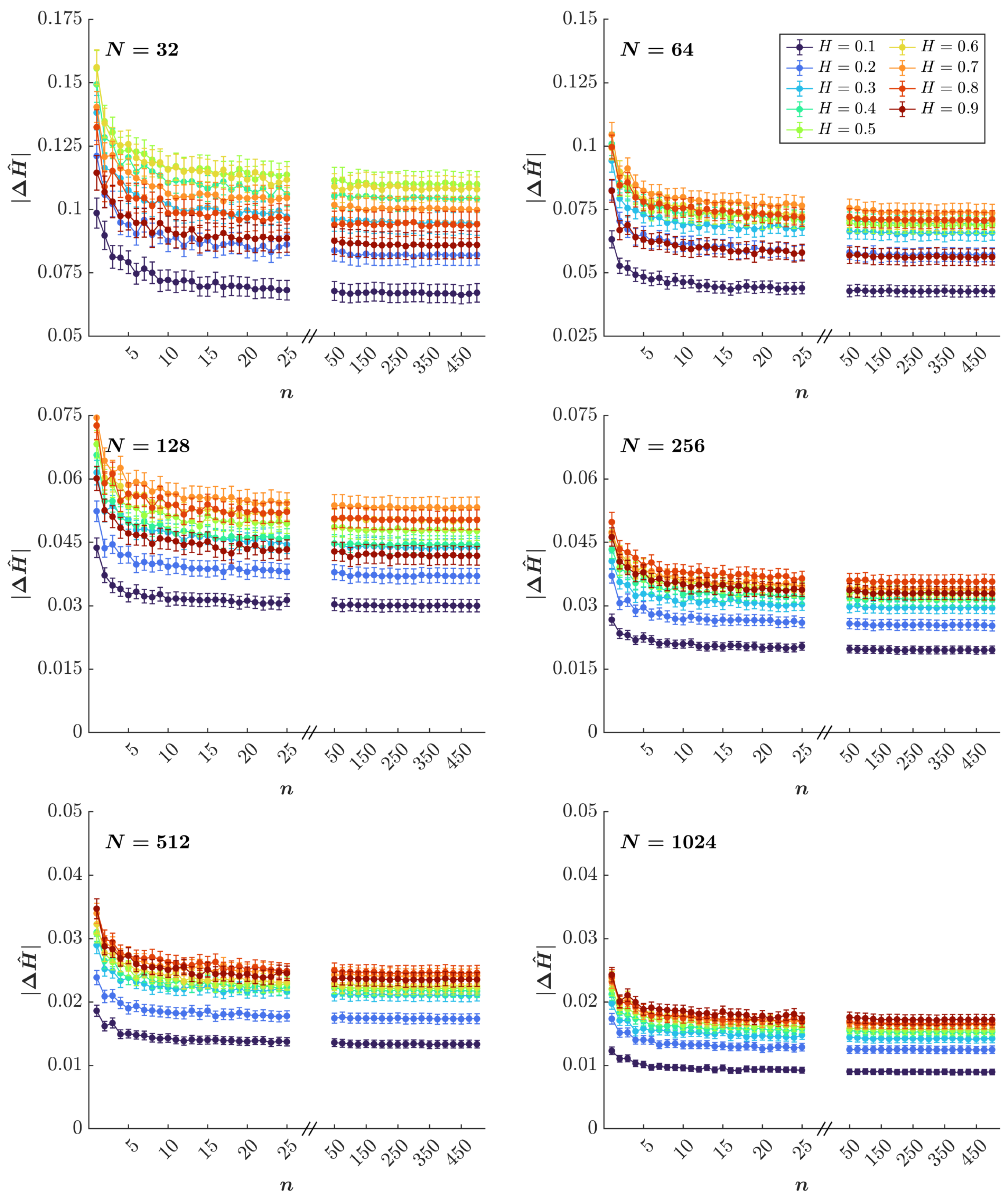
3.1. Simulation Results

Figure 1 and Figure 2 provide a summary visualization of the simulation results for each combination of the a priori known values of the Hurst exponent ($H=0.1,0.2,\dots ,0.9$), the time series length ($N=32,64,\dots ,1024$), and the sample size of H desired from the posterior distribution of H ($n=1,2,\dots ,25,50,75,\dots ,500$). As a general preview, $\widehat{H}$ estimated using the HK method closely matches the actual H for time series containing as few as 128 values (Figure 1, middle left). For shorter time series—$N=32,64$—the HK method visibly overestimates $\widehat{H}$ for smaller actual H. It underestimates $\widehat{H}$ for larger actual H (Figure 1, top left and top right respectively). Shorter time series—$N=32,64,128$—show more closely matching values of $\widehat{H}$ and H for larger posterior samples of H. Still, this trend was not apparent for longer time series—$N=256,512,1024$ (Figure 1, middle right, bottom left, and bottom right, respectively). Nonetheless, the sample size of H desired from the posterior distribution does not seem to influence the fidelity of $\widehat{H}$ for a sufficiently large sample size of H desired from the posterior distribution, that is, $n=50$.

When $N=32$, a very short time series compared to the DFA standard of >500, the estimated $\widehat{H}$ shows a large discrepancy (>0.1) with the actual H in terms of the absolute error (Figure 2, top left). Although this discrepancy sharply reduced with the sample size of H desired from the posterior distribution, almost reaching an asymptote by $n=25$, the absolute error remains considerably high even for $n=500$. For a relatively longer yet considerably short time series—$N=64$—the absolute error reduces with the sample size of H desired from the posterior distribution, reaching a lower asymptotic value of <0.1 (Figure 2, top right). However, this discrepancy is still sufficient to mask the typically observed differences in the Hurst exponent of empirical time series across two groups. For instance, the Hurst exponent of stride-to-stride interval time series during walking shows a difference of the order of $0.1$ across various task conditions (e.g., [42,43,44]). However, a discrepancy of the order of $0.1$ in the estimation of H can potentially mask these differences, resulting in false negatives in statistical tests. The trend was comparable for time series with $N=124$ except for the absolute error reaching a lower asymptotic value of ∼0.05 (Figure 2, middle left).

When $N=256$, the absolute error in the estimated $\widehat{H}$ falls within a much lower range of tolerance (<0.05) even with a very small sample of H from the posterior distribution (Figure 2, middle right). Again, the absolute error sharply reduces with n, reaching an even lower asymptotic value of ∼0.04 by $n=25$. Longer time series with $N=512$ and $N=1024$ also show similar trends except for much lower asymptotic values of absolute error: <0.03 and <0.02, respectively, by $n=25$ (Figure 2, bottom left and bottom right, respectively). In short, a relatively small sample size of H desired from the posterior distribution when using the accept–reject algorithm of the HK method suffices to estimate $\widehat{H}$ with very high accuracy. Increasing the sample size of H desired from the posterior distribution considerably increases the computational cost but confers no additional advantage in terms of the accuracy of estimating the Hurst exponent.

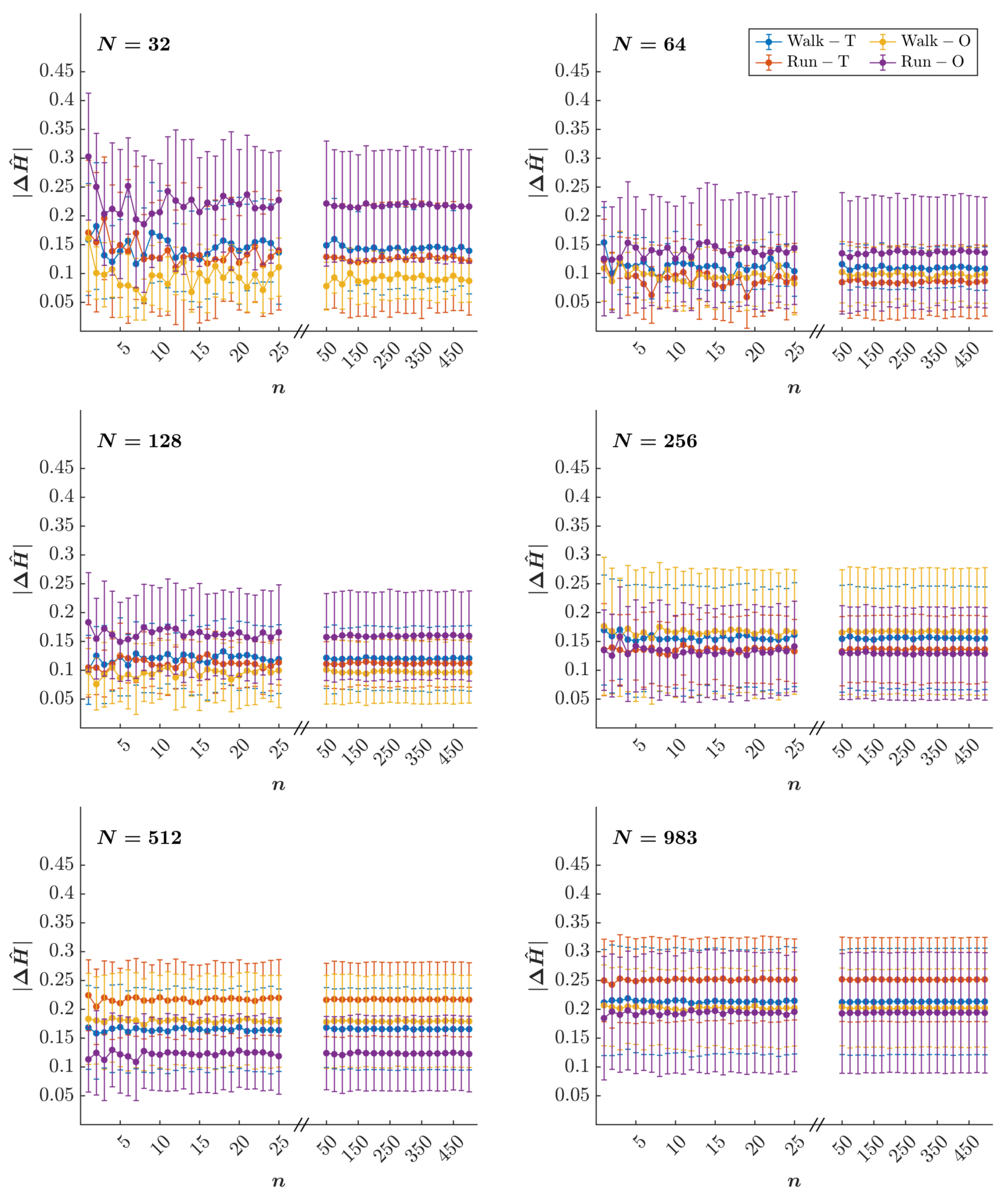
3.2. Empirical Results

Figure 3 and Figure 4 provide a summary visualization of the empirical results for stride interval time series of various lengths ($N=32,64,\dots ,983$) subjected to the HK method with the sample size of H desired from the posterior distribution of H ($n=1,2,\dots ,25,50,75,\dots ,500$). The Hurst exponent, $\widehat{H}$, estimated using the HK method for empirical time series, preserved the same rank order as the $\widehat{H}$ estimated using the first-order DFA for time series with as few as 32 data points. Figure 3 and Figure 4 clearly illustrate that the estimation of $\widehat{H}$ using the HK method is fairly stable even at 50 samples in the posterior distribution of H. This stability highlights the robustness of the HK method in maintaining consistent estimates, even with relatively small sample sizes. However, it is important to contextualize the apparent “smaller value” derived from the HK method: this result does not imply inferiority in its estimation capacity. Instead, it reflects a crucial distinction in methodology. The DFA is known to overestimate $\widehat{H}$ systematically [53,63]. Consequently, though numerically lower, the HK method’s results are more conservative and potentially closer to the actual dynamics of the time series. Thus, the “smaller value” provided by the HK method should be seen as a safeguard against the overestimation tendencies of DFA, ensuring a more reliable ranking and consistent interpretation of empirical $\widehat{H}$.

The Hurst exponent, H, provides a valuable lens for understanding the temporal structure of variability in systems like human movement. Healthy and adaptable systems exhibit an optimal balance between stability and flexibility, reflected in H values. For stride-to-stride variations in walking and running, H values close to 1 indicate an ideal temporal structure that is ordered, stable, and sufficiently variable to allow adaptability. DFA has been the standard for estimating H, with numerous studies reporting values near 1 for young and healthy adults under various task constraints, both on treadmills and overground [77,78,79,80,81,82,83,84,85,86,87,88,89,90,91,92]. Reductions in H have been documented in older adults and pathological populations [37,38,39,40,41]. These reductions correlate with decreased adaptability and an increased risk of falls [39,93,94,95,96].

While DFA has proven useful, its tendency to overestimate $\widehat{H}$ underscores the importance of comparing it with alternative methods like the HK method. The HK method provides a more conservative estimate of $\widehat{H}$, avoiding overestimation, and the figure demonstrates its robust performance in preserving the rank order of $\widehat{H}$, even with small sample sizes. Moreover, the stability of $\widehat{H}$ estimates from the HK method, evident at as few as 50 samples in the posterior distribution, suggests its reliability in capturing the underlying temporal structure. Given the empirical importance of stride-to-stride variations as a marker of task constraints and physiological health, these comparisons between DFA and the HK method offer an essential test case for refining the analytical methods used to assess movement system adaptability.

4. Discussion

The HK method offers several advantages over DFA in estimating the Hurst exponent of a time series, especially when the time series is short [65]. Nonetheless, these advantages come at the cost of computation time. The HK method is computationally expensive due to its Bayesian roots. Computationally optimizing the HK method for accurately estimating $\widehat{H}$ is, therefore, critical for promoting the adoption of the HK method over DFA for estimating the Hurst exponent in behavioral sciences. To address this issue, we have provided data on the accuracy of the Hurst exponent estimated using the HK method for synthetic time series as a function of a priori known values of H, the time series length, and the sample size of H from the posterior distribution of H—a parameter related to the Bayesian estimation that influences the accuracy of $\widehat{H}$ and computation time. A simulated sample from the posterior distribution of H as small as $n=25$ suffices to estimate the Hurst exponent with reasonable accuracy. Using a larger simulated sample from the posterior distribution of H—that is, $n>50$—provides only a marginal gain in accuracy, which might not be worth trading off with computational efficiency. Results from empirical time series on stride-to-stride intervals in humans walking and running on a treadmill and overground corroborate these findings—specifically, allowing reproduction of the rank order of $\widehat{H}$ for time series containing as few as 32 data points. We suggest balancing the simulated sample size from the posterior distribution of H with the computational resources available to the user, preferring a minimum of $n=50$ and opting for larger sample sizes based on time and resource constraints. The present results allow the reader to make judgments to optimize the Bayesian estimation of the Hurst exponent for real-time applications.

Although the present study focuses on stride interval time series from walking and running, the HK method’s applicability extends well beyond locomotor behavior. In previous work, we have applied fractal analyses, including HK-based estimation of the Hurst exponent, to behavioral and psychological time series such as response time inter-tap intervals [65]. These studies demonstrate the broader relevance of the HK method across diverse domains where long-range temporal correlations may reveal meaningful individual and task-related differences. We intentionally narrowed the empirical scope of the current manuscript to focus on optimizing computational trade-offs under well-characterized conditions, where the DFA-HK comparison has clear interpretability. Future research will extend these optimizations to other domains, including those marked by stronger nonstationarities or structural variability, to further evaluate the robustness and generalizability of the HK framework.

Empirical data pose several other issues that might undermine the accuracy of H estimated using the HK method. These issues might include strong trends [97,98,99], nonstationarities [97,100], and scaling “crossovers”—that is, long-range temporal correlations not following the same scaling law for all timescales leading to two or even multiple scaling exponents [49,50,101,102]. While these issues warrant consideration, their impact may be less severe in practice since they predominantly manifest at longer timescales. This temporal localization of anomalies suggests that the HK method remains viable for shorter-term analyses, where these effects are minimal. Nevertheless, quantifying the precise influence of trends, nonstationarities, and crossovers on estimation accuracy within a Bayesian framework represents an important direction for future research, as it would help establish clearer boundaries for the method’s reliable application.

A critical yet often overlooked factor in estimating and interpreting the Hurst exponent H is the choice of timescale over which correlations are assessed. In many real-world behavioral and physiological datasets, the underlying dynamics are not stationary across all timescales; instead, they may exhibit different correlation structures at different temporal resolutions [49,50,101,102]. This phenomenon, commonly referred to as multiscaling or scaling crossover, can result in misleading or averaged-out estimates of H when a single global exponent is assumed. While both DFA and the HK method attempt to characterize long-range temporal correlations via a single H, their sensitivity to changes in scaling behavior across timescales differs. DFA, being inherently scale-local through its box-size decomposition, may be more sensitive to scaling crossovers but also more prone to misestimations in short or noisy time series. The HK method, by contrast, assumes stationarity and a consistent correlation structure across scales, potentially smoothing over finer-scale variability. Therefore, when using the HK method in empirical settings where nonstationarities or multiple regimes are likely, it becomes crucial to consider the possibility that H may not be constant across timescales. Future work should incorporate scale-dependent extensions of the HK framework or model comparison strategies that allow users to detect and adapt to timescale-specific correlation structures. This approach would help clarify whether changes in $\widehat{H}$ reflect actual dynamical shifts or artifacts of the analysis scale, ultimately enhancing the interpretability and robustness of fractal analyses in complex systems.

The HK method demonstrates several advantages over DFA for estimating the Hurst exponent of time series, particularly for shorter datasets. Despite these advantages, the method’s wider adoption has been limited by its substantial computational demands. To address this limitation, we have systematically determined the minimum required sample size from the posterior distribution of H that maintains estimation accuracy. This optimization guidance enables researchers to select appropriate parameters that balance computational efficiency with estimation precision. Such optimization is particularly valuable for real-time applications like biofeedback paradigms and brain–computer interfaces, where rapid, successive H estimations are essential for system responsiveness.

While synthetic fGn provides a valuable testbed for benchmarking estimator performance under controlled conditions, behavioral time series often depart from these idealized assumptions, exhibiting nonstationarities, trends, and structural discontinuities. To address this, we have conducted a follow-up investigation, in which we evaluated the robustness of the HK method under various forms of empirical irregularity—including embedded contaminants and trends. These analyses reveal that, although the HK method maintains high estimation fidelity under many realistic perturbations, certain conditions (e.g., strong contamination polynomial trends) can bias $\widehat{H}$ if left uncorrected. Nonetheless, the HK method still outperforms in terms of the Hurst estimation accuracy. This underscores the importance of appropriate preprocessing and the need for diagnostic strategies when applying fractal methods to real behavioral data. We now cite this forthcoming study to provide readers with a more comprehensive understanding of the HK method’s generalizability beyond synthetic settings [76].

One limitation of the present study is that we focused primarily on the accuracy of point estimates of $\widehat{H}$ and did not characterize the variability or shape of the posterior distribution across different sample sizes. In real-world applications—especially those involving nonstationary or noisy behavioral data—understanding the spread and structure of the posterior could be crucial for interpreting uncertainty and for downstream inference. While our results suggest that $n=25$ or 50 suffices for accurate estimation of $\widehat{H}$, we did not evaluate whether smaller posterior samples systematically underestimate uncertainty. A rigorous investigation of this issue would require a dedicated analysis across a range of empirical datasets and modeling conditions, which we consider an important direction for future research. Such work would help determine when richer posterior sampling is warranted to capture underlying variability and guide more cautious interpretation of $\widehat{H}$ estimates in complex behavioral systems.

This lightweight computational profile positions the HK method as viable for embedded systems and biofeedback platforms, where rapid estimation with minimal data is often essential. Our approach resonates with broader advances in data-driven modeling that emphasize efficiency for real-time decision-making in dynamical systems. For example, Cheng et al. [103] provide a comprehensive review of machine learning methods integrated with data assimilation and uncertainty quantification to enhance predictive accuracy in high-dimensional systems. These objectives mirror our focus on improving the feasibility of estimating fractal dynamics in short time series. Similarly, Zhong et al. [104] show how reduced-order modeling and latent data assimilation enable real-time forecasting in complex, nonlinear systems such as wildfire spread. These frameworks illustrate the growing relevance of balancing model complexity with computational efficiency—an imperative our work directly addresses by identifying minimal posterior sample sizes needed to preserve accuracy in Bayesian Hurst exponent estimation. Together, these contributions help lay the groundwork for broader adoption of real-time, uncertainty-aware modeling approaches in behavioral and physiological sciences.

Importantly, while we do not report specific benchmarks for computational runtime or memory usage—given the variability introduced by different systems and implementations—all simulations and analyses were conducted on a standard consumer-grade laptop (Intel Core i7, 16GB RAM). Notably, reducing the simulated posterior sample size to as few as 25 substantially lowers the computational load, making the Bayesian HK method accessible for real-time or near-real-time applications. This lightweight computational profile positions the method as viable for embedded systems and biofeedback platforms, where rapid estimation with minimal data is often essential.

An important consideration in any Bayesian framework is the sensitivity of posterior estimates to the choice of prior distribution. In this study, we adopted a uniform prior over the interval $(0,1)$ for the Hurst exponent H, consistent with the original HK method [64]. This uninformative prior ensures generality of the Bayesian Hurst estimation and avoids biasing the estimation toward any particular value of H. Our simulations suggest that, under this prior, the HK method reliably converges to accurate estimates of $\widehat{H}$ across a wide range of time series lengths and posterior sample sizes. Importantly, we observed no systematic bias or inflation of estimation error that would indicate prior-related distortion, even under challenging conditions such as short time series or extreme values of H. Nonetheless, in contexts where prior domain knowledge about H exists—such as cardiovascular physiology or climate modeling—informative priors (e.g., Beta distributions) could be incorporated to improve estimation under small-sample or noisy conditions. Future work should systematically evaluate the impact of such prior choices, particularly in data-limited applications, to balance estimation fidelity with domain-specific expectations.

The implications of the present findings extend well beyond behavioral and movement sciences. The Hurst exponent has a long history of use in diverse domains such as finance, climate science, and physiology, where long-range temporal correlations are used to characterize underlying system dynamics and assess risk, resilience, or pathology. In finance, H helps quantify the degree of memory in asset returns or volatility processes [105], informing portfolio optimization and risk management strategies [106]. In climate science, H is used to model persistence in temperature and precipitation records [107], with implications for forecasting and understanding climate variability. In physiology, H is a key descriptor of temporal complexity in cardiovascular, respiratory, and neural signals [17], and has been shown to differentiate between healthy and pathological states [35,108]. By demonstrating that accurate estimation of $\widehat{H}$ is achievable with small sample sizes and reduced computational cost, the current results may inform new methodologies in these fields—particularly in high-frequency trading, real-time climate monitoring, or ambulatory health monitoring—where data are noisy, short, and computational resources may be constrained [101]. The HK method’s balance of accuracy and efficiency, therefore, positions it as a powerful tool across disciplines where detecting changes in long-range dependence is essential for diagnostics, prediction, or control.

To further illustrate the practical utility of the optimized HK method, consider a real-time clinical monitoring scenario in Parkinson’s disease. Gait variability in Parkinsonian patients is known to increase in irregularity as motor symptoms progress, and the Hurst exponent has been proposed as a marker for quantifying long-range temporal correlations in stride intervals [109,110]. A wearable system equipped with inertial sensors could stream stride interval time series to a mobile device, where the HK method—optimized to use as few as $n=25$ posterior samples—could rapidly estimate $\widehat{H}$ in near real time. This would allow for continuous, on-the-fly assessment of motor stability, enabling early detection of deterioration, personalized medication titration, or adaptive cueing interventions [111,112]. Similarly, in cardiovascular monitoring, the method could be applied to heart rate variability data gathered from consumer-grade wearables to flag early signs of autonomic imbalance in at-risk populations [108,113]. These examples underscore the feasibility and clinical relevance of low-latency, high-fidelity fractal analysis using the HK method, especially in applications where computational efficiency and data limitations have previously precluded its use.

References

1. Mandelbrot, B.B.; Wallis, J.R. Computer experiments with fractional Gaussian noises: Part 1, Averages and variances. Water Resour. Res. 1969, 5, 228–241. [Google Scholar] [CrossRef]
2. Hurst, H.E. Long-term storage capacity of reservoirs. Trans. Am. Soc. Civ. Eng. 1951, 116, 770–799. [Google Scholar] [CrossRef]
3. Efstathiou, M.; Varotsos, C. On the altitude dependence of the temperature scaling behaviour at the global troposphere. Int. J. Remote Sens. 2010, 31, 343–349. [Google Scholar] [CrossRef]
4. Ivanova, K.; Ausloos, M. Application of the detrended fluctuation analysis (DFA) method for describing cloud breaking. Phys. A Stat. Mech. Its Appl. 1999, 274, 349–354. [Google Scholar] [CrossRef]
5. Tatli, H.; Dalfes, H.N. Long-time memory in drought via detrended fluctuation analysis. Water Resour. Manag. 2020, 34, 1199–1212. [Google Scholar] [CrossRef]
6. Alvarez-Ramirez, J.; Alvarez, J.; Rodriguez, E. Short-term predictability of crude oil markets: A detrended fluctuation analysis approach. Energy Econ. 2008, 30, 2645–2656. [Google Scholar] [CrossRef]
7. Grau-Carles, P. Empirical evidence of long-range correlations in stock returns. Phys. A Stat. Mech. Its Appl. 2000, 287, 396–404. [Google Scholar] [CrossRef]
8. Ivanov, P.C.; Yuen, A.; Podobnik, B.; Lee, Y. Common scaling patterns in intertrade times of US stocks. Phys. Rev. E 2004, 69, 056107. [Google Scholar] [CrossRef]
9. Liu, Y.; Cizeau, P.; Meyer, M.; Peng, C.K.; Stanley, H.E. Correlations in economic time series. Phys. A Stat. Mech. Its Appl. 1997, 245, 437–440. [Google Scholar] [CrossRef]
10. Liu, Y.; Gopikrishnan, P.; Cizeau, P.; Meyer, M.; Peng, C.-K.; Stanley, H.E. Statistical properties of the volatility of price fluctuations. Phys. Rev. E 1999, 60, 1390. [Google Scholar] [CrossRef]
11. Alados, C.L.; Huffman, M.A. Fractal long-range correlations in behavioural sequences of wild chimpanzees: A non-invasive analytical tool for the evaluation of health. Ethology 2000, 106, 105–116. [Google Scholar] [CrossRef]
12. Bee, M.A.; Kozich, C.E.; Blackwell, K.J.; Gerhardt, H.C. Individual variation in advertisement calls of territorial male green frogs, Rana clamitans: Implications for individual discrimination. Ethology 2001, 107, 65–84. [Google Scholar] [CrossRef]
13. Buldyrev, S.; Dokholyan, N.; Goldberger, A.; Havlin, S.; Peng, C.K.; Stanley, H.; Viswanathan, G. Analysis of DNA sequences using methods of statistical physics. Phys. A Stat. Mech. Its Appl. 1998, 249, 430–438. [Google Scholar] [CrossRef]
14. Mantegna, R.N.; Buldyrev, S.V.; Goldberger, A.L.; Havlin, S.; Peng, C.K.; Simons, M.; Stanley, H.E. Linguistic features of noncoding DNA sequences. Phys. Rev. Lett. 1994, 73, 3169. [Google Scholar] [CrossRef]
15. Peng, C.K.; Buldyrev, S.; Goldberger, A.; Havlin, S.; Simons, M.; Stanley, H. Finite-size effects on long-range correlations: Implications for analyzing DNA sequences. Phys. Rev. E 1993, 47, 3730. [Google Scholar] [CrossRef]
16. Castiglioni, P.; Faini, A. A fast DFA algorithm for multifractal multiscale analysis of physiological time series. Front. Physiol. 2019, 10, 115. [Google Scholar] [CrossRef]
17. Goldberger, A.L.; Amaral, L.A.; Hausdorff, J.M.; Ivanov, P.C.; Peng, C.K.; Stanley, H.E. Fractal dynamics in physiology: Alterations with disease and aging. Proc. Natl. Acad. Sci. USA 2002, 99, 2466–2472. [Google Scholar] [CrossRef] [PubMed]
18. Hardstone, R.; Poil, S.S.; Schiavone, G.; Jansen, R.; Nikulin, V.V.; Mansvelder, H.D.; Linkenkaer-Hansen, K. Detrended fluctuation analysis: A scale-free view on neuronal oscillations. Front. Physiol. 2012, 3, 450. [Google Scholar] [CrossRef] [PubMed]
19. Peng, C.K.; Mietus, J.; Hausdorff, J.; Havlin, S.; Stanley, H.E.; Goldberger, A.L. Long-range anticorrelations and non-Gaussian behavior of the heartbeat. Phys. Rev. Lett. 1993, 70, 1343. [Google Scholar] [CrossRef]
20. Delignières, D.; Torre, K.; Bernard, P.L. Transition from persistent to anti-persistent correlations in postural sway indicates velocity-based control. PLoS Comput. Biol. 2011, 7, e1001089. [Google Scholar] [CrossRef]
21. Duarte, M.; Sternad, D. Complexity of human postural control in young and older adults during prolonged standing. Exp. Brain Res. 2008, 191, 265–276. [Google Scholar] [CrossRef] [PubMed]
22. Lin, D.; Seol, H.; Nussbaum, M.A.; Madigan, M.L. Reliability of COP-based postural sway measures and age-related differences. Gait Posture 2008, 28, 337–342. [Google Scholar] [CrossRef]
23. Chen, Y.; Ding, M.; Kelso, J.S. Long memory processes (1/fα type) in human coordination. Phys. Rev. Lett. 1997, 79, 4501. [Google Scholar] [CrossRef]
24. Diniz, A.; Wijnants, M.L.; Torre, K.; Barreiros, J.; Crato, N.; Bosman, A.M.; Hasselman, F.; Cox, R.F.; Van Orden, G.C.; Delignières, D. Contemporary theories of 1/f noise in motor control. Hum. Mov. Sci. 2011, 30, 889–905. [Google Scholar] [CrossRef]
25. Allegrini, P.; Menicucci, D.; Bedini, R.; Fronzoni, L.; Gemignani, A.; Grigolini, P.; West, B.J.; Paradisi, P. Spontaneous brain activity as a source of ideal 1/f noise. Phys. Rev. E 2009, 80, 061914. [Google Scholar] [CrossRef]
26. Gilden, D.L.; Thornton, T.; Mallon, M.W. 1/f noise in human cognition. Science 1995, 267, 1837–1839. [Google Scholar] [CrossRef]
27. Kello, C.T.; Brown, G.D.; Ferrer-i Cancho, R.; Holden, J.G.; Linkenkaer-Hansen, K.; Rhodes, T.; Van Orden, G.C. Scaling laws in cognitive sciences. Trends Cogn. Sci. 2010, 14, 223–232. [Google Scholar] [CrossRef] [PubMed]
28. Stephen, D.G.; Stepp, N.; Dixon, J.A.; Turvey, M. Strong anticipation: Sensitivity to long-range correlations in synchronization behavior. Phys. A Stat. Mech. Its Appl. 2008, 387, 5271–5278. [Google Scholar] [CrossRef]
29. Van Orden, G.C.; Holden, J.G.; Turvey, M.T. Self-organization of cognitive performance. J. Exp. Psychol. Gen. 2003, 132, 331–350. [Google Scholar] [CrossRef]
30. Mangalam, M.; Conners, J.D.; Kelty-Stephen, D.G.; Singh, T. Fractal fluctuations in muscular activity contribute to judgments of length but not heaviness via dynamic touch. Exp. Brain Res. 2019, 237, 1213–1226. [Google Scholar] [CrossRef]
31. Mangalam, M.; Chen, R.; McHugh, T.R.; Singh, T.; Kelty-Stephen, D.G. Bodywide fluctuations support manual exploration: Fractal fluctuations in posture predict perception of heaviness and length via effortful touch by the hand. Hum. Mov. Sci. 2020, 69, 102543. [Google Scholar] [CrossRef] [PubMed]
32. Mangalam, M.; Carver, N.S.; Kelty-Stephen, D.G. Global broadcasting of local fractal fluctuations in a bodywide distributed system supports perception via effortful touch. Chaos Solitons Fractals 2020, 135, 109740. [Google Scholar] [CrossRef]
33. Ashkenazy, Y.; Lewkowicz, M.; Levitan, J.; Havlin, S.; Saermark, K.; Moelgaard, H.; Thomsen, P.B. Discrimination between healthy and sick cardiac autonomic nervous system by detrended heart rate variability analysis. Fractals 1999, 7, 85–91. [Google Scholar] [CrossRef]
34. Ho, K.K.; Moody, G.B.; Peng, C.K.; Mietus, J.E.; Larson, M.G.; Levy, D.; Goldberger, A.L. Predicting survival in heart failure case and control subjects by use of fully automated methods for deriving nonlinear and conventional indices of heart rate dynamics. Circulation 1997, 96, 842–848. [Google Scholar] [CrossRef] [PubMed]
35. Peng, C.K.; Havlin, S.; Hausdorff, J.; Mietus, J.; Stanley, H.; Goldberger, A. Fractal mechanisms and heart rate dynamics: Long-range correlations and their breakdown with disease. J. Electrocardiol. 1995, 28, 59–65. [Google Scholar] [CrossRef]
36. Bartsch, R.; Plotnik, M.; Kantelhardt, J.W.; Havlin, S.; Giladi, N.; Hausdorff, J.M. Fluctuation and synchronization of gait intervals and gait force profiles distinguish stages of Parkinson’s disease. Phys. A Stat. Mech. Its Appl. 2007, 383, 455–465. [Google Scholar] [CrossRef]
37. Hausdorff, J.M.; Mitchell, S.L.; Firtion, R.; Peng, C.K.; Cudkowicz, M.E.; Wei, J.Y.; Goldberger, A.L. Altered fractal dynamics of gait: Reduced stride-interval correlations with aging and Huntington’s disease. J. Appl. Physiol. 1997, 82, 262–269. [Google Scholar] [CrossRef]
38. Hausdorff, J.M.; Ashkenazy, Y.; Peng, C.K.; Ivanov, P.C.; Stanley, H.E.; Goldberger, A.L. When human walking becomes random walking: Fractal analysis and modeling of gait rhythm fluctuations. Phys. A Stat. Mech. Its Appl. 2001, 302, 138–147. [Google Scholar] [CrossRef]
39. Hausdorff, J.M. Gait dynamics, fractals and falls: Finding meaning in the stride-to-stride fluctuations of human walking. Hum. Mov. Sci. 2007, 26, 555–589. [Google Scholar] [CrossRef]
40. Herman, T.; Giladi, N.; Gurevich, T.; Hausdorff, J. Gait instability and fractal dynamics of older adults with a “cautious” gait: Why do certain older adults walk fearfully? Gait Posture 2005, 21, 178–185. [Google Scholar] [CrossRef]
41. Kobsar, D.; Olson, C.; Paranjape, R.; Hadjistavropoulos, T.; Barden, J.M. Evaluation of age-related differences in the stride-to-stride fluctuations, regularity and symmetry of gait using a waist-mounted tri-axial accelerometer. Gait Posture 2014, 39, 553–557. [Google Scholar] [CrossRef] [PubMed]
42. Mangalam, M.; Skiadopoulos, A.; Siu, K.C.; Mukherjee, M.; Likens, A.; Stergiou, N. Leveraging a virtual alley with continuously varying width modulates step width variability during self-paced treadmill walking. Neurosci. Lett. 2022, 793, 136966. [Google Scholar] [CrossRef] [PubMed]
43. Raffalt, P.C.; Stergiou, N.; Sommerfeld, J.H.; Likens, A.D. The temporal pattern and the probability distribution of visual cueing can alter the structure of stride-to-stride variability. Neurosci. Lett. 2021, 763, 136193. [Google Scholar] [CrossRef] [PubMed]
44. Raffalt, P.C.; Sommerfeld, J.H.; Stergiou, N.; Likens, A.D. Stride-to-stride time intervals are independently affected by the temporal pattern and probability distribution of visual cues. Neurosci. Lett. 2023, 792, 136909. [Google Scholar] [CrossRef]
45. Kaipust, J.P.; McGrath, D.; Mukherjee, M.; Stergiou, N. Gait variability is altered in older adults when listening to auditory stimuli with differing temporal structures. Ann. Biomed. Eng. 2013, 41, 1595–1603. [Google Scholar] [CrossRef]
46. Marmelat, V.; Duncan, A.; Meltz, S.; Meidinger, R.L.; Hellman, A.M. Fractal auditory stimulation has greater benefit for people with Parkinson’s disease showing more random gait pattern. Gait Posture 2020, 80, 234–239. [Google Scholar] [CrossRef]
47. Vaz, J.R.; Knarr, B.A.; Stergiou, N. Gait complexity is acutely restored in older adults when walking to a fractal-like visual stimulus. Hum. Mov. Sci. 2020, 74, 102677. [Google Scholar] [CrossRef]
48. Peng, C.K.; Buldyrev, S.V.; Havlin, S.; Simons, M.; Stanley, H.E.; Goldberger, A.L. Mosaic organization of DNA nucleotides. Phys. Rev. E 1994, 49, 1685. [Google Scholar] [CrossRef]
49. Peng, C.K.; Havlin, S.; Stanley, H.E.; Goldberger, A.L. Quantification of scaling exponents and crossover phenomena in nonstationary heartbeat time series. Chaos 1995, 5, 82–87. [Google Scholar] [CrossRef]
50. Bashan, A.; Bartsch, R.; Kantelhardt, J.W.; Havlin, S. Comparison of detrending methods for fluctuation analysis. Phys. A Stat. Mech. Its Appl. 2008, 387, 5080–5090. [Google Scholar] [CrossRef]
51. Grech, D.; Mazur, Z. Statistical properties of old and new techniques in detrended analysis of time series. Acta Phys. Pol. Ser. B 2005, 36, 2403. [Google Scholar]
52. Almurad, Z.M.; Delignières, D. Evenly spacing in detrended fluctuation analysis. Phys. A Stat. Mech. Its Appl. 2016, 451, 63–69. [Google Scholar] [CrossRef]
53. Delignieres, D.; Ramdani, S.; Lemoine, L.; Torre, K.; Fortes, M.; Ninot, G. Fractal analyses for ‘short’ time series: A re-assessment of classical methods. J. Math. Psychol. 2006, 50, 525–544. [Google Scholar] [CrossRef]
54. Dlask, M.; Kukal, J. Hurst exponent estimation from short time series. Signal Image Video Process. 2019, 13, 263–269. [Google Scholar] [CrossRef]
55. Katsev, S.; L’Heureux, I. Are Hurst exponents estimated from short or irregular time series meaningful? Comput. Geosci. 2003, 29, 1085–1089. [Google Scholar] [CrossRef]
56. Marmelat, V.; Meidinger, R.L. Fractal analysis of gait in people with Parkinson’s disease: Three minutes is not enough. Gait Posture 2019, 70, 229–234. [Google Scholar] [CrossRef]
57. Ravi, D.K.; Marmelat, V.; Taylor, W.R.; Newell, K.M.; Stergiou, N.; Singh, N.B. Assessing the temporal organization of walking variability: A systematic review and consensus guidelines on detrended fluctuation analysis. Front. Physiol. 2020, 11, 562. [Google Scholar] [CrossRef]
58. Roume, C.; Ezzina, S.; Blain, H.; Delignières, D. Biases in the simulation and analysis of fractal processes. Comput. Math. Methods Med. 2019, 2019, 4025305. [Google Scholar] [CrossRef]
59. Schaefer, A.; Brach, J.S.; Perera, S.; Sejdić, E. A comparative analysis of spectral exponent estimation techniques for 1/fβ processes with applications to the analysis of stride interval time series. J. Neurosci. Methods 2014, 222, 118–130. [Google Scholar] [CrossRef]
60. Yuan, Q.; Gu, C.; Weng, T.; Yang, H. Unbiased detrended fluctuation analysis: Long-range correlations in very short time series. Phys. A Stat. Mech. Its Appl. 2018, 505, 179–189. [Google Scholar] [CrossRef]
61. Höll, M.; Kantz, H. The relationship between the detrendend fluctuation analysis and the autocorrelation function of a signal. Eur. Phys. J. B 2015, 88, 1–7. [Google Scholar] [CrossRef]
62. Kiyono, K. Establishing a direct connection between detrended fluctuation analysis and Fourier analysis. Phys. Rev. E 2015, 92, 042925. [Google Scholar] [CrossRef]
63. Stroe-Kunold, E.; Stadnytska, T.; Werner, J.; Braun, S. Estimating long-range dependence in time series: An evaluation of estimators implemented in R. Behav. Res. Methods 2009, 41, 909–923. [Google Scholar] [CrossRef]
64. Tyralis, H.; Koutsoyiannis, D. A Bayesian statistical model for deriving the predictive distribution of hydroclimatic variables. Clim. Dyn. 2014, 42, 2867–2883. [Google Scholar] [CrossRef]
65. Likens, A.D.; Mangalam, M.; Wong, A.Y.; Charles, A.C.; Mills, C. Better than DFA? A Bayesian method for estimating the Hurst exponent in behavioral sciences. arXiv 2023, arXiv:2301.11262. [Google Scholar]
66. Koutsoyiannis, D. Climate change, the Hurst phenomenon, and hydrological statistics. Hydrol. Sci. J. 2003, 48, 3–24. [Google Scholar] [CrossRef]
67. Golub, G.H.; Van Loan, C.F. Matrix Computations; John Hopkins University Press: Baltimore, MD, USA, 2013. [Google Scholar]
68. Robert, C.P.; Casella, G.; Casella, G. Monte Carlo Statistical Methods; Springer: New York, NY, USA, 1999; Volume 2. [Google Scholar]
69. Gelman, A.; Carlin, J.B.; Stern, H.S.; Rubin, D.B. Bayesian Data Analysis; Chapman and Hall/CRC: Boca Raton, FL, USA, 1995. [Google Scholar]
70. R Core Team. R: A Language and Environment for Statistical Computing. R Version 4.0.4 2024. Available online: https://www.R-project.org/ (accessed on 31 March 2023).
71. Tyralis, H. Package ‘HKprocess’. R Package Version 0.1-1 2022. Available online: https://cran.r-project.org/package=HKprocess (accessed on 31 March 2023).
72. Davies, R.B.; Harte, D. Tests for Hurst effect. Biometrika 1987, 74, 95–101. [Google Scholar] [CrossRef]
73. Likens, A.; Wiltshire, T. fractalRegression: An R Package for Fractal Analyses and Regression 2021. Available online: https://github.com/aaronlikens/fractalRegression (accessed on 31 March 2023).
74. Wilson, T.; Mangalam, M.; Stergiou, N.; Likens, A. Multifractality in stride-to-stride variations reveals that walking entails tuning and adjusting movements more than running. Hum. Mov. Sci. 2023, 3, 1294545. [Google Scholar]
75. Martin, P.E.; Rothstein, D.E.; Larish, D.D. Effects of age and physical activity status on the speed-aerobic demand relationship of walking. J. Appl. Physiol. 1992, 73, 200–206. [Google Scholar] [CrossRef]
76. Mangalam, M.; Likens, A.D. Precision in brief: The Bayesian Hurst-Kolmogorov method for assessing long-range temporal correlations in short behavioral time series. Entropy 2025, 27, 500. [Google Scholar] [CrossRef]
77. Agresta, C.E.; Goulet, G.C.; Peacock, J.; Housner, J.; Zernicke, R.F.; Zendler, J.D. Years of running experience influences stride-to-stride fluctuations and adaptive response during step frequency perturbations in healthy distance runners. Gait Posture 2019, 70, 376–382. [Google Scholar] [CrossRef] [PubMed]
78. Bellenger, C.R.; Arnold, J.B.; Buckley, J.D.; Thewlis, D.; Fuller, J.T. Detrended fluctuation analysis detects altered coordination of running gait in athletes following a heavy period of training. J. Sci. Med. Sport 2019, 22, 294–299. [Google Scholar] [CrossRef] [PubMed]
79. Brahms, C.M.; Zhao, Y.; Gerhard, D.; Barden, J.M. Long-range correlations and stride pattern variability in recreational and elite distance runners during a prolonged run. Gait Posture 2020, 92, 487–492. [Google Scholar] [CrossRef]
80. Bollens, B.; Crevecoeur, F.; Nguyen, V.; Detrembleur, C.; Lejeune, T. Does human gait exhibit comparable and reproducible long-range autocorrelations on level ground and on treadmill? Gait Posture 2010, 32, 369–373. [Google Scholar] [CrossRef]
81. Ducharme, S.W.; Liddy, J.J.; Haddad, J.M.; Busa, M.A.; Claxton, L.J.; van Emmerik, R.E. Association between stride time fractality and gait adaptability during unperturbed and asymmetric walking. Hum. Mov. Sci. 2018, 58, 248–259. [Google Scholar] [CrossRef]
82. Fairley, J.A.; Sejdić, E.; Chau, T. The effect of treadmill walking on the stride interval dynamics of children. Hum. Mov. Sci. 2010, 29, 987–998. [Google Scholar] [CrossRef] [PubMed]
83. Fuller, J.T.; Amado, A.; van Emmerik, R.E.; Hamill, J.; Buckley, J.D.; Tsiros, M.D.; Thewlis, D. The effect of footwear and footfall pattern on running stride interval long-range correlations and distributional variability. Gait Posture 2016, 44, 137–142. [Google Scholar] [CrossRef]
84. Fuller, J.T.; Bellenger, C.R.; Thewlis, D.; Arnold, J.; Thomson, R.L.; Tsiros, M.D.; Robertson, E.Y.; Buckley, J.D. Tracking performance changes with running-stride variability when athletes are functionally overreached. Int. J. Sport. Physiol. Perform. 2017, 12, 357–363. [Google Scholar] [CrossRef]
85. Hausdorff, J.M.; Peng, C.K.; Ladin, Z.; Wei, J.Y.; Goldberger, A.L. Is walking a random walk? Evidence for long-range correlations in stride interval of human gait. J. Appl. Physiol. 1995, 78, 349–358. [Google Scholar] [CrossRef]
86. Hausdorff, J.M.; Purdon, P.L.; Peng, C.K.; Ladin, Z.; Wei, J.Y.; Goldberger, A.L. Fractal dynamics of human gait: Stability of long-range correlations in stride interval fluctuations. J. Appl. Physiol. 1996, 80, 1448–1457. [Google Scholar] [CrossRef]
87. Jordan, K.; Challis, J.H.; Newell, K.M. Long range correlations in the stride interval of running. Gait Posture 2006, 24, 120–125. [Google Scholar] [CrossRef] [PubMed]
88. Jordan, K.; Challis, J.H.; Cusumano, J.P.; Newell, K.M. Stability and the time-dependent structure of gait variability in walking and running. Hum. Mov. Sci. 2009, 28, 113–128. [Google Scholar] [CrossRef] [PubMed]
89. Lindsay, T.R.; Noakes, T.D.; McGregor, S.J. Effect of treadmill versus overground running on the structure of variability of stride timing. Percept. Mot. Skills 2014, 118, 331–346. [Google Scholar] [CrossRef] [PubMed]
90. Mangalam, M.; Kelty-Stephen, D.G.; Sommerfeld, J.H.; Stergiou, N.; Likens, A.D. Temporal organization of stride-to-stride variations contradicts predictive models for sensorimotor control of footfalls during walking. PLoS ONE 2023, 18, e0290324. [Google Scholar] [CrossRef]
91. Nakayama, Y.; Kudo, K.; Ohtsuki, T. Variability and fluctuation in running gait cycle of trained runners and non-runners. Gait Posture 2010, 31, 331–335. [Google Scholar] [CrossRef]
92. Terrier, P.; Dériaz, O. Kinematic variability, fractal dynamics and local dynamic stability of treadmill walking. J. Neuroeng. Rehabil. 2011, 8, 12. [Google Scholar] [CrossRef]
93. Hausdorff, J.M.; Rios, D.A.; Edelberg, H.K. Gait variability and fall risk in community-living older adults: A 1-year prospective study. Arch. Phys. Med. Rehabil. 2001, 82, 1050–1056. [Google Scholar] [CrossRef]
94. Johansson, J.; Nordström, A.; Nordström, P. Greater fall risk in elderly women than in men is associated with increased gait variability during multitasking. J. Am. Med Dir. Assoc. 2016, 17, 535–540. [Google Scholar] [CrossRef]
95. Paterson, K.; Hill, K.; Lythgo, N. Stride dynamics, gait variability and prospective falls risk in active community dwelling older women. Gait Posture 2011, 33, 251–255. [Google Scholar] [CrossRef]
96. Toebes, M.J.; Hoozemans, M.J.; Furrer, R.; Dekker, J.; van Dieën, J.H. Local dynamic stability and variability of gait are associated with fall history in elderly subjects. Gait Posture 2012, 36, 527–531. [Google Scholar] [CrossRef]
97. Bryce, R.; Sprague, K. Revisiting detrended fluctuation analysis. Sci. Rep. 2012, 2, 315. [Google Scholar] [CrossRef] [PubMed]
98. Hu, K.; Ivanov, P.C.; Chen, Z.; Carpena, P.; Stanley, H.E. Effect of trends on detrended fluctuation analysis. Phys. Rev. E 2001, 64, 011114. [Google Scholar] [CrossRef] [PubMed]
99. Horvatic, D.; Stanley, H.E.; Podobnik, B. Detrended cross-correlation analysis for non-stationary time series with periodic trends. Europhys. Lett. 2011, 94, 18007. [Google Scholar] [CrossRef]
100. Chen, Z.; Ivanov, P.C.; Hu, K.; Stanley, H.E. Effect of nonstationarities on detrended fluctuation analysis. Phys. Rev. E 2002, 65, 041107. [Google Scholar] [CrossRef] [PubMed]
101. Kantelhardt, J.W.; Koscielny-Bunde, E.; Rego, H.H.; Havlin, S.; Bunde, A. Detecting long-range correlations with detrended fluctuation analysis. Phys. A Stat. Mech. Its Appl. 2001, 295, 441–454. [Google Scholar] [CrossRef]
102. Kelty-Stephen, D.G.; Palatinus, K.; Saltzman, E.; Dixon, J.A. A tutorial on multifractality, cascades, and interactivity for empirical time series in ecological science. Ecol. Psychol. 2013, 25, 1–62. [Google Scholar] [CrossRef]
103. Cheng, S.; Quilodrán-Casas, C.; Ouala, S.; Farchi, A.; Liu, C.; Tandeo, P.; Fablet, R.; Lucor, D.; Iooss, B.; Brajard, J.; et al. Machine learning with data assimilation and uncertainty quantification for dynamical systems: A review. IEEE/CAA J. Autom. Sin. 2023, 10, 1361–1387. [Google Scholar] [CrossRef]
104. Zhong, C.; Cheng, S.; Kasoar, M.; Arcucci, R. Reduced-order digital twin and latent data assimilation for global wildfire prediction. Nat. Hazards Earth Syst. Sci. 2023, 23, 1755–1768. [Google Scholar] [CrossRef]
105. Mandelbrot, B.B.; Hudson, R.L. The (mis) Behaviour of Markets: A Fractal View of Risk, Ruin and Reward; Basic Books: New York, NY, USA, 2004. [Google Scholar]
106. Cont, R. Long range dependence in financial markets. In Fractals in Engineering: New Trends in Theory and Applications; Lévy-Véhel, J., Lutton, E., Eds.; Springer: London, UK, 2005; pp. 159–179. [Google Scholar] [CrossRef]
107. Fraedrich, K.; Blender, R. Scaling of atmosphere and ocean temperature correlations in observations and climate models. Phys. Rev. Lett. 2003, 90, 108501. [Google Scholar] [CrossRef]
108. Kiyono, K.; Hayano, J.; Kwak, S.; Watanabe, E.; Yamamoto, Y. Non-Gaussianity of low frequency heart rate variability and sympathetic activation: Lack of increases in multiple system atrophy and Parkinson disease. Front. Physiol. 2012, 3, 34. [Google Scholar] [CrossRef]
109. Hausdorff, J.M. Gait dynamics in Parkinson’s disease: Common and distinct behavior among stride length, gait variability, and fractal-like scaling. Chaos Interdiscip. J. Nonlinear Sci. 2009, 19, 026113. [Google Scholar] [CrossRef] [PubMed]
110. Kirchner, M.; Schubert, P.; Liebherr, M.; Haas, C.T. Detrended fluctuation analysis and adaptive fractal analysis of stride time data in Parkinson’s disease: Stitching together short gait trials. PLoS ONE 2014, 9, e85787. [Google Scholar] [CrossRef] [PubMed]
111. Del Din, S.; Godfrey, A.; Mazzà, C.; Lord, S.; Rochester, L. Free-living monitoring of Parkinson’s disease: Lessons from the field. Mov. Disord. 2016, 31, 1293–1313. [Google Scholar] [CrossRef] [PubMed]
112. Espay, A.J.; Bonato, P.; Nahab, F.B.; Maetzler, W.; Dean, J.M.; Klucken, J.; Eskofier, B.M.; Merola, A.; Horak, F.; Lang, A.E.; et al. Technology in Parkinson’s disease: Challenges and opportunities. Mov. Disord. 2016, 31, 1272–1282. [Google Scholar] [CrossRef]
113. Perkiömäki, J.S. Heart rate variability and non-linear dynamics in risk stratification. Front. Physiol. 2011, 2, 81. [Google Scholar] [CrossRef]
Figure 1. The Hurst exponent, H ^ , for synthetic fGn time series estimated using the HK method closely matches the actual H for time series containing as few as 128 values. Each panel plots the M e a n H for 1000 synthetic time series with length N = 32 , 64 , 128 , 256 , 512 , 1024 ; a priori known values of H ranging from 0.1 to 0.9 ; and the sample size of H desired from the posterior distribution of H, n = 1 , 2 , , 25 , 50 , 75 , , 500 . Horizontal colored lines indicate the actual H. Error bars indicate 95 % CI across 1000 simulations.
Axioms 14 00421 g001
Figure 2. The absolute error in the estimation of the Hurst exponent, H ^ , for synthetic fGn time series using the HK method sharply reduces with the sample size of H desired from the posterior distribution of H, reaching an asymptote at n = 50 . Using a larger simulated sample from the posterior distribution of H—that is, n > 50 —does not influence the accuracy of the estimated H. Each panel plots the M e a n absolute error in the estimated H for 1000 synthetic time series with length N = 32 , 64 , 128 , 256 , 512 , 1024 ; a priori known values of H ranging from 0.1 to 0.9 ; and the sample size of H desired from the posterior distribution of H, n = 1 , 2 , , 25 , 50 , 75 , , 500 . Error bars indicate 95 % CI across 1000 simulations.
Axioms 14 00421 g002
Figure 3. The Hurst exponent, H ^ , for empirical time series estimated using the HK method preserves the same order as the H ^ estimated using the first-order DFA for time series containing as few as 32 data points. Each panel plots the M e a n  H for stride interval time series with length N = 32 , 64 , 128 , 256 , 512 , 983 and the sample size of H desired from the posterior distribution of H, n = 1 , 2 , , 25 , 50 , 75 , , 500 . The larger circles indicate the H ^ estimated using the first-order DFA. Error bars indicate 95 % CI across the study group size of 8 participants.
Axioms 14 00421 g003
Figure 4. The absolute difference in the estimation of the Hurst exponent, H ^ , for empirical stride interval time series using the HK method; the first-order DFA stabilizes with the sample size of H desired from the posterior distribution of H by n = 50 . Using a larger simulated sample from the posterior distribution of H—that is, n > 50 —does not influence the relative accuracy of the estimated H. Each panel plots the M e a n absolute difference in the estimated H for empirical stride interval time series with length N = 32 , 64 , 128 , 256 , 512 , 983 and the sample size of H desired from the posterior distribution of H, n = 1 , 2 , , 25 , 50 , 75 , , 500 . Error bars indicate 95 % CI across the study group size of 8 participants.
Axioms 14 00421 g004
Disclaimer/Publisher’s Note: The statements, opinions and data contained in all publications are solely those of the individual author(s) and contributor(s) and not of MDPI and/or the editor(s). MDPI and/or the editor(s) disclaim responsibility for any injury to people or property resulting from any ideas, methods, instructions or products referred to in the content.