Dynamic Event-Triggered Interval Observer-Based Fault Detection for a Class of Nonlinear Cyber–Physical Systems with Disturbance

Abstract

This paper investigates the problem of interval estimation and fault detection for nonlinear cyber–physical systems (CPSs) subject to disturbances and random actuator/sensor faults. First, with the purpose of reducing the burden of data transmission, we introduce the dynamic event-triggered mechanism (DETM). For systems violating the non-negativity condition, a coordinate transformation method is applied to enhance the design flexibility. Then, the dynamic event-triggered interval observer (DETIO) is constructed and the effectiveness of DETIO is validated by demonstrating the ultimate uniform boundedness of the error system. The fault detection is achieved by considering faults in the CPSs and continuously monitoring residual signals. Finally, two numerical simulations under both faulty and fault-free conditions are shown to prove the effectiveness and superiority of the designed DETIO-based fault detection method.

1. Introduction

In past few decades, CPSs have been widely studied by the scientific community. CPSs are intelligent systems that deeply integrate the capabilities of computation, communication, and physical processes [1]. Owing to their unique capability to bridge the physical and cyber worlds, CPSs have already been applied in many areas, e.g., the electric power industry [2] and water systems [3]. However, as CPSs grow more complex and face unknown disturbances, the tasks of estimating states and detecting faults efficiently also pose challenges. For the state estimation problems in CPSs, one common method is the observer design technique. For example, ref. [4] investigated a switched observer for CPSs via a set cover approach. Ref. [5] focused on a sliding mode observer design for CPSs. Ref. [6] analyzed the estimation stability in the network system under attack. Furthermore, the interval observer (IO), as an effective tool for obtaining the estimated state boundaries of the system with unknown bounded disturbances and measurement noises, is also introduced to CPSs [7,8].

Meanwhile, due to the high demand for communication and data transmission in CPSs, the event-triggered mechanism (ETM) has been introduced and gained significant research interest. The fundamental principle of ETM is to decide the trigger through system states, instead of the conventional mechanism that triggers actions with fixed sampling intervals. The authors of [9] introduced a periodic technique to ETM and also applied it to both static state-feedback and dynamic output-based controllers. In [10], researchers combined the ETM and observer technique for the control of positive nonlinear multi-agent systems. To further reduce the burden while ensuring the performance of the system, the dynamic event-triggered mechanism was introduced [11,12,13]. Ref. [11] imported an interval dynamic variable which forms the DETM. Researchers in [12] investigated a dynamic periodic ETM to decrease asynchronous behavior generated from nonuniform communication delays. Ref. [13] applied a DETM to investigate the interval estimation problem for Euler–Lagrange systems under stealthy attack. Moreover, in order to precisely estimate the states with uncertain disturbance during communications, the event-triggered interval observer (ETIO) was proposed in [14]. Furthermore, ref. [15] took advantage of DETM to estimate the boundaries of the system with unknown but bounded disturbance and noise using a zonotope-based approach. Hence, ETM offers a new approach to save communication resources for solving the estimation problem.

In addition, for CPSs with actuator/sensor faults, ensuring system stability requires effective fault detection. The main fault detection approaches can be broadly classified into model-based [16,17], data-driven [18,19,20], and hybrid approaches [21]. Among these, the IO-based fault detection method has gained much attention, considering its strong robustness against uncertainties. For example, ref. [22] proposed an IO-based fault detection approach with unknown input for CPSs under attacks. Similarly, in [23], for a T-S fuzzy system, the fault detection method was established via a zonotope-based IO. Ref. [24] designed a sliding mode IO to detect faults and eliminate uncertainties with the existence of the measurement noise in high-speed railway traction motors. However, as far as the authors are aware, research on fault detection based on interval estimation, which integrates DETM in CPSs, remains limited.

As a result, a DETIO design is developed in this paper for fault detection problems of a class of nonlinear CPSs. The DETIO fault detection design relies on its stability, which is mainly derived from a combination of the Lyapunov stability theory and the positive system theory. Moreover, in this paper, we discuss the utilization of the coordinate transformation method under the case where the error system is not non-negative. The contributions presented in this paper can be briefly described as follows:

(1)

The DETM that possesses a dynamic interval variable, which depends on the system states, is introduced to save communication resources in CPSs; compared to the static ETM, it can save more network resources while guaranteeing the stability of the systems.

(2)

A DETIO is designed for CPSs under actuator/sensor faults. The mentioned DETIO approach can accurately obtain the bounded estimation of the states without wasting additional data transmission resources.

(3)

The designed DETIO is applied to fault detection in CPSs. By bounding the state estimates with the DETM, this fault detection method reduces computational load and ensures the robustness of the system.

The remainder of this paper is summarized as follows. Section 2 focuses on the preliminaries and problem statements. Section 3 gives the DETIO frame design. Section 4 gives some numerical examples to simulate the circumstances of fault-free and under faults, respectively. Finally, we present the conclusion in Section 5.

Notations: Given a matrix $z=\left[\begin{array}{c}{z}_{ij}\end{array}\right]\in {\mathbb{R}}^{m\times n}$, $z\ge 0$ if $z_{ij}\ge 0$. For a matrix $E\in {\mathbb{R}}^{m\times m}$ and $E^T=E$, $E\prec 0(E\succ 0)$ indicates that E is a negative (positive) definite matrix. Moreover, given a matrix $A\in {\mathbb{R}}^{m\times n}$, we define that $A^{+}=max\{A,0\}$ and $A^{-}=A^{+}-A$.

2. Preliminaries and Problem Statement

The nonlinear CPS model in this paper is considered as follows:

$$\left\{\begin{array}{c}\begin{array}{cc}\hfill & x(k+1)=Ax\left(k\right)+Bu\left(k\right)+F\left(x\right(k\left)\right)+D\delta \left(k\right)+Ef\left(k\right),\hfill \\ \hfill & y\left(k\right)=Cx\left(k\right),\hfill \end{array}\end{array}\right.$$

(1)

where $x\in {\mathbb{R}}^n$, $y\in {\mathbb{R}}^n$ and $u\in {\mathbb{R}}^n$ represent the state, output, and control input of the system, respectively. $\delta \in {\mathbb{R}}^n$ is an unknown disturbance, $f\in {\mathbb{R}}^n$ denotes the actuator fault. The matrices A, B, D, C, and E, along with the nonlinear function $F\left(x\right)$, with appropriate dimensions are known. To save network resources in a CPS, the DETM is introduced to detect faults. In this study, we propose the following DETM for the system (1):

$$t_0=0,t_{k+1}=inf\left\{t>t_k|\Gamma \left(k\right)+\alpha [\eta y^T\left(k\right)y\left(k\right)-e_y^T\left(k\right)e_y\left(k\right)\le 0]\right\},$$

(2)

where $\alpha \ge 0$, $0<\eta <0.5$. And the non-negative function $\Gamma \left(k\right)$ satisfies the following equation:

$$\Gamma (k+1)=-\lambda \Gamma \left(k\right)+\eta y^T\left(k\right)y\left(k\right)-e_y^T\left(k\right)e_y\left(k\right),$$

(3)

where $\Gamma \left(0\right)={\Gamma }_0\ge 0$ and $\lambda$ is a positive scalar.

Assumption 1.

Suppose that there are constant vectors ${\delta }_k^{+}$ and ${\delta }_k^{-}$; then, the disturbance ${\delta }_k$ holds:

$${\delta }_k^{-}\le {\delta }_k\le {\delta }_k^{+}.$$

(4)

Assumption 2.

Given a function $f(x,y)$, if, for any $(x,y_1),(x,y_2)$, we have a Lipschitz constant c that satisfies the following inequality:

$$\parallel f(x,y_1)-f(x,y_2)\parallel \le c\parallel y_1-y_2\parallel .$$

(5)

Then, the function $f(x,y)$ is Lipschitz continuous in y with constant c.

Lemma 1

([25]). For a given Lipschitz function $F\left(x\right)$ that is globally differentiable, the following equation holds:

$$F\left(x\right)=g_1\left(x\right)-g_2\left(x\right).$$

(6)

where $g_1\left(x\right)$ and $g_2\left(x\right)$ are two globally differentiable and increasing Lipschitz functions.

Lemma 2

([25]). Consider the function $F\left(x\right)$ in Lemma 1. The Lipschitz function $\overline{F}(x_m,x_n)$ exists and is globally differentiable, such that

$$F\left(x\right)=\overline{F}(x,x),$$

$${\displaystyle \frac{\partial \overline{F}}{\partial x_m}\ge 0,\frac{\partial \overline{F}}{\partial x_n}\le 0.}$$

From Lemmas 1 and 2, the lower and upper boundaries subject to the nonlinear function $G(x,x)$ can be derived as

$$\overline{F}(x^{-},x^{+})\le F(x,x)\le \overline{F}(x^{+},x^{-}).$$

(7)

Lemma 3

([26]). For a vector $v\in {\mathbb{R}}^{n\times 1}$, given a constant matrix $M\in {\mathbb{R}}^{n\times n}$ and the vector v satisfying $v^{-}\le v\le v^{+}$,

$$M^{+}{v}^{-}-M^{-}{v}^{+}\le Mv\le M^{+}{v}^{+}-M^{-}{v}^{-}.$$

(8)

Lemma 4

([25]). For the functions $F\left(x\right)$, $\overline{F}(x^{-},x^{+})$ and $\overline{F}(x^{+},x^{-})$ mentioned above, there exist known constant matrices $F_a,F_b,F_c,$ and $F_d$ such that

$$\left\{\begin{array}{c}\begin{array}{c}\overline{F}(x^{+},x^{-})-F(x,x)\le F_a\overline{e}+F_b\underline{e},\hfill \\ F(x,x)-\overline{F}(x^{-},x^{+})\le F_c\overline{e}+F_d\underline{e},\hfill \end{array}\end{array}\right.$$

(9)

where $\overline{e}=x^{+}-x$ and $\overline{e}=x-x^{-}$.

Lemma 5

([27]). Given the following systems

$$\left\{\begin{array}{c}\begin{array}{c}{x}_{k+1}=K{x}_k+F\left(x_k\right),\hfill \\ x_0\ge 0,\hfill \end{array}\end{array}\right.$$

(10)

where the constant matrix K is non-negative and the function $F\left(x_k\right)\ge 0$, we can obtain $x_k\ge 0$ for all $k\ge 0$.

Lemma 6

([28]). If there are two arbitrary matrices G, $V\in {\mathbb{R}}^{n\times n}$ and a constant β, we have

$$G^{T}V+V^{T}G\le {\displaystyle \frac{1}{\beta }}{G}^{T}PG+\beta V^T{P}^{-1}V,$$

(11)

where the matrix $P\succ 0$ and $\beta >0$.

Remark 1.

For the above DETM in (2) and (3), let $\alpha \ge 0$, $\eta >0$, and ${\Gamma }_0\ge 0$. Then, for $\forall k>0$, the dynamic interval variable $\Gamma \left(k\right)$ holds:

$$\Gamma \left(k\right)\ge 0.$$

(12)

Moreover, for cases where $\alpha =0$, the DETM will degrade to the static event-triggered mechanism.

3. Main Results

3.1. Design of the Fault Detection DETIO

According to the discussion above, for system (1), we propose the following fault detection DETIO:

$$\left\{\begin{array}{c}\begin{array}{cc}\hfill x^{+}(k+1)=& A{x}^{+}\left(k\right)+Bu\left(k\right)+\overline{F}(x^{+}\left(k\right),x^{-}\left(k\right))+{\mu }^{+}\left(k\right)\hfill \\ \hfill & +\overline{h}\left(k\right)+L(y_{{\tau }_p}\left(k\right)-C{x}^{+}\left(k\right)),\hfill \end{array}\\ x^{-}(k+1)=A{x}^{-}\left(k\right)+Bu\left(k\right)+\overline{F}(x^{-}\left(k\right),x^{+}\left(k\right))+{\mu }^{-}\left(k\right)\\ +\underline{h}\left(k\right)+L(y_{{\tau }_p}\left(k\right)-C{x}^{-}\left(k\right)),\end{array}\right.$$

(13)

$$\left\{\begin{array}{c}\begin{array}{c}\hfill r^{+}\left(k\right)=y\left(k\right)-C{x}^{-}\left(k\right),\\ \hfill r^{-}\left(k\right)=y\left(k\right)-C{x}^{+}\left(k\right),\end{array}\end{array}\right.$$

(14)

where $x^{+}\left(k\right)$ and $x^{-}\left(k\right)$ are estimates of $x\left(k\right)$, ${\mu }^{+}\left(k\right)=D^{+}{\delta }^{+}\left(k\right)-D^{-}{\delta }^{-}\left(k\right)$ and ${\mu }^{-}\left(k\right)=D^{+}{\delta }^{-}\left(k\right)-D^{-}{\delta }^{+}\left(k\right)$, $\overline{h}\left(k\right)=L^{-}{e}_y^{+}\left(k\right)-L^{+}{e}_y^{-}\left(k\right)$, and $\underline{h}\left(k\right)=L^{-}{e}_y^{-}\left(k\right)-L^{+}{e}_y^{+}\left(k\right)$. $r^{+}$ and $r^{-}$ are the interval residual vectors used to detect the fault. The gain L of the interval observer will be discussed in the next part.

Theorem 1.

If $A-LC$ satisfies the non-negativity condition and $x^{-}\left(0\right)\le x\left(0\right)\le x^{+}\left(0\right)$. For all $k\in \mathbb{N}$, the following inequality holds:

$$x^{-}\left(k\right)\le x\left(k\right)\le x^{+}\left(k\right).$$

(15)

Proof. 

Define $e^{+}\left(k\right)=x^{+}\left(k\right)-x\left(k\right)$ and $e^{-}\left(k\right)=x\left(k\right)-x^{-}\left(k\right)$; then, we can deduce that

$$\left\{\begin{array}{c}\begin{array}{cc}\hfill e^{+}(k+1)=& (A-LC)e^{+}\left(k\right)-F\left(x\left(k\right)\right)+\overline{F}(x^{+}\left(k\right),x^{-}\left(k\right))\hfill \\ & +e_{\delta }^{+}\left(k\right)+L{e}_y\left(k\right)+\overline{h}\left(k\right)-Ef\left(k\right),\hfill \\ \hfill e^{-}(k+1)=& (A-LC)e^{-}\left(k\right)-\overline{F}(x^{-}\left(k\right),x^{+}\left(k\right))+F\left(x\left(k\right)\right)\hfill \\ & +e_{\delta }^{-}\left(k\right)-\underline{h}\left(k\right)-L{e}_y\left(k\right)+Ef\left(k\right),\hfill \end{array}\end{array}\right.$$

(16)

where $e_{\delta }^{+}\left(k\right)={\mu }^{+}\left(k\right)-D\delta \left(k\right)$ and $e_{\delta }^{-}\left(k\right)=D\delta \left(k\right)-{\mu }^{-}\left(k\right)$. By Lemma 3, we can obtain that $e_{\delta }^{-}\left(k\right)\ge 0$, $e_{\delta }^{+}\left(k\right)\ge 0$. Similarly,

$$\left\{\begin{array}{c}L{e}_y\left(k\right)+\overline{h}\left(k\right)=L{e}_y\left(k\right)-(L^{+}{e}_y^{-}\left(k\right)-L^{-}{e}_y^{+}\left(k\right))\ge 0,\\ -\underline{h}\left(k\right)-L{e}_y\left(k\right)=(L^{+}{e}_y^{+}\left(k\right)-L^{-}{e}_y^{-}\left(k\right))-L{e}_y\left(k\right)\ge 0.\end{array}\right.$$

(17)

If $A-LC$ satisfies the non-negative condition, and the initial conditions (15) hold, then the positivity of the error system (16) can be proven according to Lemma 5. Therefore, we can also deduce that $x^{-}\left(k\right)\le x\left(k\right)\le x^{+}\left(k\right),\forall k\ge 0$, which completes the proof.   □

3.2. Coordinate Transformation-Based Fault Detection DETIO Design

Given a situation that $A-LC$ is not a non-negative matrix, we can adopt the coordinate transformation technique to build the DETIO for CPSs. Denote $w\left(k\right)=Hx\left(k\right)$, $\overline{A}=HA{H}^{-1}$, $\overline{B}=HB$, $\overline{C}=C{H}^{-1}$, $\overline{D}=HD$, $\overline{E}=HE$, and we can rewrite the system (3) as follows:

$$\left\{\begin{array}{c}\begin{array}{c}w(k+1)=\overline{A}w\left(k\right)+\overline{B}u\left(k\right)+HF\left(H^{-1}w\left(k\right)\right)+\overline{D}\delta \left(k\right)+\overline{E}f\left(k\right),\hfill \\ y\left(k\right)=\overline{C}w\left(k\right).\hfill \end{array}\end{array}\right.$$

(18)

To obtain the estimated boundaries of $F\left(x\right)$, it is denoted that

$$\left\{\begin{array}{c}\begin{array}{c}\phi (w^{+}\left(k\right),w^{-}\left(k\right))=\overline{F}(H_r^{+}{w}^{+}\left(k\right)-H_r^{-}{w}^{-}\left(k\right),H_r^{+}{w}^{-}\left(k\right)-H_r^{-}{w}^{+}\left(k\right)),\hfill \\ \phi (w^{-}\left(k\right),w^{+}\left(k\right))=\overline{F}(H_r^{+}{w}^{-}\left(k\right)-H_r^{-}{w}^{+}\left(k\right),H_r^{+}{w}^{+}\left(k\right)-H_r^{-}{w}^{-}\left(k\right)),\hfill \end{array}\end{array}\right.$$

(19)

where $H_r=H^{-1}$, $w^{-}\left(k\right)$, and $w^{+}\left(k\right)$ represent the lower and upper estimations of $w\left(k\right)$, respectively. According to Lemmas 3 and 4, the following inequalities are deduced as

$$\begin{array}{cc}\hfill {\overline{F}}_w(w^{-},w^{+})& =H^{+}\phi (w^{-},w^{+})-H^{-}\phi (w^{+},w^{-})\le H\overline{F}\left(H^{-1}w\right)\hfill \\ \hfill & \le H^{+}\phi (w^{+},w^{-})-H^{-}\phi (w^{-},w^{+})={\overline{F}}_w(w^{+},w^{-}).\hfill \end{array}$$

(20)

Then, the fault detection DETIO framework is constructed as follows:

$$\left\{\begin{array}{c}\begin{array}{cc}\hfill w^{+}(k+1)=& \overline{A}{w}^{+}\left(k\right)+\overline{B}u\left(k\right)+{\overline{F}}_w(w^{+}\left(k\right),w^{-}\left(k\right))+d^{+}\left(k\right)\hfill \\ \hfill & +\overline{\eta }\left(k\right)+L(y_{{\tau }_p}\left(k\right)-\overline{C}{w}^{+}\left(k\right)),\hfill \\ \hfill w^{-}(k+1)=& \overline{A}{w}^{-}\left(k\right)+\overline{B}u\left(k\right)+{\overline{F}}_w(w^{-}\left(k\right),w^{+}\left(k\right))+d^{-}\left(k\right)\hfill \\ \hfill & +\underline{\eta }\left(k\right)+L(y_{{\tau }_p}\left(k\right)-\overline{C}{w}^{-}\left(k\right)),\hfill \end{array}\end{array}\right.$$

(21)

$$\left\{\begin{array}{c}\begin{array}{c}\hfill {\overline{r}}^{+}\left(k\right)=y\left(k\right)-\overline{C}{w}^{-}\left(k\right),\\ \hfill {\overline{r}}^{-}\left(k\right)=y\left(k\right)-\overline{C}{w}^{+}\left(k\right),\end{array}\end{array}\right.$$

(22)

where

$$\left\{\begin{array}{c}\begin{array}{cc}\hfill d^{+}\left(k\right)=& {\overline{D}}^{+}{\delta }^{+}\left(k\right)-{\overline{D}}^{-}{\delta }^{-}\left(k\right)\hfill \\ \hfill d^{-}\left(k\right)=& {\overline{D}}^{+}{\delta }^{-}\left(k\right)-{\overline{D}}^{-}{\delta }^{+}\left(k\right)\hfill \end{array}\end{array}\right.and\left\{\begin{array}{c}\begin{array}{c}\hfill \overline{\eta }\left(k\right)=L^{-}{e}_y^{+}\left(k\right)-L^{+}{e}_y^{-}\left(k\right)\\ \hfill \underline{\eta }\left(k\right)=L^{-}{e}_y^{-}\left(k\right)-L^{+}{e}_y^{+}\left(k\right)\end{array}\end{array}\right..$$

(23)

Since the transformation matrix H is nonsingular, using the initial condition, it can be obtained that

$$w^{-}\left(0\right)\le w\left(0\right)\le w^{+}\left(0\right),$$

(24)

where

$$\left\{\begin{array}{c}\begin{array}{c}{w}^{+}\left(0\right)=H^{+}{x}^{-}\left(0\right)-H^{-}{x}^{+}\left(0\right),\hfill \\ w^{-}\left(0\right)=H^{+}{x}^{+}\left(0\right)-H^{-}{x}^{-}\left(0\right).\hfill \end{array}\end{array}\right.$$

(25)

Defining ${ϵ}^{+}\left(k\right)=w^{+}\left(k\right)-w\left(k\right)$ and ${ϵ}^{-}\left(k\right)=w\left(k\right)-w^{-}\left(k\right)$. Then, the dynamic errors can be deduced as

$$\left\{\begin{array}{c}\begin{array}{cc}\hfill {ϵ}^{+}(k+1)=& (\overline{A}-L\overline{C}){ϵ}^{+}\left(k\right)+{\overline{F}}_w(w{\left(k\right)}^{+},w{\left(k\right)}^{-})-H\overline{F}\left(H^{-1}w\left(k\right)\right)\hfill \\ \hfill & +e_{\Delta }^{+}\left(k\right)+L{e}_y\left(k\right)+\overline{\eta }\left(k\right)-\overline{E}f\left(k\right),\hfill \end{array}\\ {ϵ}^{-}(k+1)=(\overline{A}-L\overline{C}){ϵ}^{-}\left(k\right)+H\overline{F}\left(H^{-1}w\left(k\right)\right)-{\overline{F}}_w(w{\left(k\right)}^{-},w{\left(k\right)}^{+})\hfill \\ +e_{\Delta }^{-}\left(k\right)-L{e}_y\left(k\right)-\underline{\eta }\left(k\right)+\overline{E}f\left(k\right),\end{array}\right.$$

(26)

where $e_{\Delta }^{+}\left(k\right)=d^{+}\left(k\right)-\overline{D}\delta \left(k\right)$ and $e_{\Delta }^{-}\left(k\right)=\overline{D}\delta \left(k\right)-d^{-}\left(k\right)$.

Remark 2.

For CPSs that do not satisfy the non-negative condition, through the coordinate transformation method, we can still construct a matrix H, causing $A-LC$ to be non-negative after transformation. This approach enhances the flexibility and reduces the constraints of designing a DETIO for CPSs.

Theorem 2.

Given a non-negative matrix $\overline{A}-L\overline{C}$, under the cases where the initial condition after the coordinate transformation holds, we have

$$w^{-}\left(k\right)\le w\left(k\right)\le w^{+}\left(k\right).$$

(27)

Proof. 

If $\overline{A}-L\overline{C}$ is a non-negative matrix, by Lemma 5, the dynamic error system (26) can be deduced to be positive. From Lemma 2 and (24), since the matrix H is nonsingular, we can obtain the following inequalities:

$$w^{-}\left(k\right)\le w\left(k\right)\le w^{+}\left(k\right),k\ge 0.$$

(28)

Thus, the proof of Theorem 2 is finished.    □

Subsequently, by denoting ${\xi }_k={\left[{{ϵ}^{+}\left(k\right)}^T{{ϵ}^{-}\left(k\right)}^T\right]}^T$, and according to (18) and (26), we have

$$\begin{array}{cc}\hfill {\xi }_{k+1}=& M{\xi }_k+\check{F}+\check{\omega }+\check{\epsilon }+\check{E}\hfill \end{array}$$

(29)

where

$$M=\left[\begin{array}{cc}\overline{A}-L\overline{C}& 0\\ 0& \overline{A}-L\overline{C}\end{array}\right],$$

$$\check{F}=\left[\begin{array}{c}{\overline{F}}_w(w^{+}\left(k\right),w^{-}\left(k\right))-H\overline{F}\left(H^{-1}w\left(k\right)\right)\\ H\overline{F}\left(H^{-1}w\left(k\right)\right)-{\overline{F}}_w(w^{-}\left(k\right),w^{+}\left(k\right))\end{array}\right],\check{\omega }=\left[\begin{array}{c}{\overline{D}}^{+}{d}^{+}-{\overline{D}}^{-}{d}^{-}-\overline{D}d\\ \overline{D}d-{\overline{D}}^{+}{d}^{-}+{\overline{D}}^{-}{d}^{+}\end{array}\right],$$

$$\check{\epsilon }=\left[\begin{array}{c}L{e}_y+L^{-}{e}_y^{+}-L^{+}{e}_y^{-}\\ -L{e}_y+L^{+}{e}_y^{+}-L^{-}{e}_y^{-}\end{array}\right],\check{E}=\left[\begin{array}{c}-\overline{E}f\\ \overline{E}f\end{array}\right].$$

Theorem 3.

Given positive constants λ and ${\gamma }_i(i=1,2,\dots ,10)$, and under Assumptions 1 and 2, if there exists a positive-definite and symmetric matrix P that satisfies the following inequalities:

$$\begin{array}{c}\hfill \Pi =\left[\begin{array}{ccc}{\Pi }_1& 0& 0\\ *& {\Pi }_2& 0\\ *& *& {\Pi }_3\end{array}\right]\prec 0,\end{array}$$

(30)

where

$$\begin{array}{cc}\hfill & {\Pi }_1=(1+{\gamma }_1+{\gamma }_2+{\gamma }_3)M^{T}PM+(1+{\displaystyle \frac{1}{{\gamma }_1}}+{\gamma }_4+{\gamma }_5){\widehat{F}}^{T}P\widehat{F}-(1-\lambda )P,\hfill \\ \hfill & {\Pi }_2=-I,\hfill \\ \hfill & {\Pi }_3=\eta {\overline{C}}^T\overline{C}-\rho I,\hfill \end{array}$$

$$\widehat{F}=\left[\begin{array}{cc}{F}_a& F_b\\ F_c& F_d\end{array}\right],$$

then the system (26) is uniformly ultimately bounded (UUB).

Proof. 

Choose the candidate Lyapunov function for the systems given by (3) and (18) as follows:

$$W\left(k\right)=V\left(k\right)+\Gamma \left(k\right),$$

(31)

where $V\left(k\right)={\xi }_k^{T}P{\xi }_k$, and then it can be obtained that

$$\begin{array}{cc}\hfill W(k+1)=& {[M{\xi }_k+\check{F}+\check{\omega }+\check{\epsilon }+\check{E}]}^{T}P[M{\xi }_k+\check{F}+\check{\omega }+\check{\epsilon }+\check{E}]+{\Gamma }_{k+1}\hfill \\ \hfill =& {\left(M{\xi }_k\right)}^{T}P\left(M{\xi }_k\right)+{\left(M{\xi }_k\right)}^{T}P\check{F}+{\left(M{\xi }_k\right)}^{T}P\check{\omega }+{\left(M{\xi }_k\right)}^{T}P\check{\epsilon }+{\left(M{\xi }_k\right)}^{T}P\check{E}\hfill \\ \hfill & +{\left(\check{F}\right)}^{T}PM{\xi }_k+{\left(\check{\omega }\right)}^{T}PM{\xi }_k+{\left(\check{\epsilon }\right)}^{T}PM{\xi }_k+{\left(\check{E}\right)}^{T}PM\hfill \\ \hfill & +{\left(\check{F}\right)}^{T}P\check{\omega }+{\left(\check{\omega }\right)}^{T}P\check{F}+{\left(\check{F}\right)}^{T}P\check{\epsilon }+{\left(\check{\epsilon }\right)}^{T}P\check{F}+{\left(\check{F}\right)}^{T}P\check{E}+{\left(\check{E}\right)}^{T}P\check{F}\hfill \\ \hfill & +{\left(\check{\omega }\right)}^{T}P\check{\epsilon }+{\left(\check{\epsilon }\right)}^{T}P\check{\omega }+{\left(\check{\omega }\right)}^{T}P\check{E}+{\left(\check{E}\right)}^{T}P\check{\stackrel{ˇ}{\omega }}+{\left(\check{\epsilon }\right)}^{T}P\check{E}+{\left(\check{E}\right)}^{T}P\check{\epsilon }\hfill \\ \hfill & +{\left(\check{F}\right)}^{T}P\check{F}+{\left(\check{\omega }\right)}^{T}P\check{\omega }+{\left(\check{\epsilon }\right)}^{T}P\check{\epsilon }+{\left(\check{E}\right)}^{T}P\check{E}\hfill \\ \hfill & -\lambda \Gamma \left(k\right)+\eta y^T\left(k\right)y\left(k\right)-e_y^T\left(k\right)e_y\left(k\right).\hfill \end{array}$$

Then, the following are denoted:

$$\begin{array}{cccc}\hfill M_1\left(k\right)& ={\left(M{\xi }_k\right)}^{T}P\check{F},\hfill & \hfill & M_2\left(k\right)={\left(M{\xi }_k\right)}^{T}P\check{\omega },\hfill \\ \hfill M_3\left(k\right)& ={\left(M{\xi }_k\right)}^{T}P\check{\epsilon },\hfill & \hfill & M_4\left(k\right)={\left(M{\xi }_k\right)}^{T}P\check{E},\hfill \\ \hfill M_5\left(k\right)& ={\check{F}}^{T}P\check{\omega },\hfill & \hfill & M_6\left(k\right)={\check{F}}^{T}P\check{\epsilon },\hfill \\ \hfill M_7\left(k\right)& ={\check{F}}^{T}P\check{E},\hfill & \hfill & M_8\left(k\right)={\check{\omega }}^{T}P\check{\epsilon },\hfill \\ \hfill M_9\left(k\right)& ={\check{\omega }}^{T}P\check{\epsilon },\hfill & \hfill & M_{10}\left(k\right)={\check{\epsilon }}^{T}P\check{E}.\hfill \end{array}$$

(32)

From Lemma 6, we can deduce that

$$\begin{array}{cc}\hfill & M_1\left(k\right)+M_1^T\left(k\right)\le {\gamma }_1{\left(M{\xi }_k\right)}^{T}PM{\xi }_k+{\displaystyle \frac{1}{{\gamma }_1}}{\left(\check{F}\right)}^{T}P\check{F},\hfill \\ \hfill & M_2\left(k\right)+M_2^T\left(k\right)\le {\gamma }_2{\left(M{\xi }_k\right)}^{T}PM{\xi }_k+{\displaystyle \frac{1}{{\gamma }_2}}{\left(\check{\omega }\right)}^{T}P\check{\omega },\hfill \\ \hfill & M_3\left(k\right)+M_3^T\left(k\right)\le {\gamma }_3{\left(M{\xi }_k\right)}^{T}PM{\xi }_k+{\displaystyle \frac{1}{{\gamma }_3}}{\left(\check{\epsilon }\right)}^{T}P\check{\epsilon },\hfill \\ \hfill & M_4\left(k\right)+M_4^T\left(k\right)\le {\gamma }_4{\left(M{\xi }_k\right)}^{T}PM{\xi }_k+{\displaystyle \frac{1}{{\gamma }_4}}{\left(\check{E}\right)}^{T}P\check{E},\hfill \\ \hfill & M_5\left(k\right)+M_5^T\left(k\right)\le {\gamma }_5{\left(\check{F}\right)}^{T}P\check{F}+{\displaystyle \frac{1}{{\gamma }_5}}{\left(\check{\omega }\right)}^{T}P\check{\omega },\hfill \\ \hfill & M_6\left(k\right)+M_6^T\left(k\right)\le {\gamma }_6{\left(\check{F}\right)}^{T}P\check{F}+{\displaystyle \frac{1}{{\gamma }_6}}{\left(\check{\epsilon }\right)}^{T}P\check{\epsilon },\hfill \\ \hfill & M_7\left(k\right)+M_7^T\left(k\right)\le {\gamma }_7{\left(\check{F}\right)}^{T}P\check{F}+{\displaystyle \frac{1}{{\gamma }_7}}{\left(\check{E}\right)}^{T}P\check{E},\hfill \\ \hfill & M_8\left(k\right)+M_8^T\left(k\right)\le {\gamma }_8{\left(\check{\omega }\right)}^{T}P\check{\omega }+{\displaystyle \frac{1}{{\gamma }_8}}{\left(\check{\epsilon }\right)}^{T}P\check{\epsilon },\hfill \\ \hfill & M_9\left(k\right)+M_9^T\left(k\right)\le {\gamma }_9{\left(\check{\omega }\right)}^{T}P\check{\omega }+{\displaystyle \frac{1}{{\gamma }_9}}{\left(\check{E}\right)}^{T}P\check{E},\hfill \\ \hfill & M_{10}\left(k\right)+M_{10}^T\left(k\right)\le {\gamma }_{10}{\left(\check{\epsilon }\right)}^{T}P\check{\epsilon }+{\displaystyle \frac{1}{{\gamma }_{10}}}{\left(\check{E}\right)}^{T}P\check{E}.\hfill \end{array}$$

(33)

Thus, we can derive that

$$\begin{array}{cc}\hfill \Delta W_k& =W(k+1)-W\left(k\right)\hfill \\ \hfill & \le (1+{\gamma }_1+{\gamma }_2+{\gamma }_3+{\gamma }_4){\left(M{\xi }_k\right)}^{T}PM{\xi }_k+(1+{\displaystyle \frac{1}{{\gamma }_1}}+{\gamma }_5+{\gamma }_6+{\gamma }_7){\left(\check{F}\right)}^{T}P\check{F}\hfill \\ \hfill & +(1+{\displaystyle \frac{1}{{\gamma }_2}}+{\displaystyle \frac{1}{{\gamma }_5}}+{\gamma }_8+{\gamma }_9){\left(\check{\omega }\right)}^{T}P\check{\omega }+(1+{\displaystyle \frac{1}{{\gamma }_3}}+{\displaystyle \frac{1}{{\gamma }_6}}+{\displaystyle \frac{1}{{\gamma }_8}}+{\gamma }_{10}){\left(\check{\epsilon }\right)}^{T}P\check{\epsilon }\hfill \\ \hfill & +(1+{\displaystyle \frac{1}{{\gamma }_4}}+{\displaystyle \frac{1}{{\gamma }_7}}+{\displaystyle \frac{1}{{\gamma }_9}}+{\displaystyle \frac{1}{{\gamma }_{10}}}){(\check{E})}^{T}P\check{E}-{\xi }_k^{T}P{\xi }_k-(\lambda +1)\Gamma \left(k\right)\hfill \\ \hfill & +\eta y^T\left(k\right)y\left(k\right)-e_y^T\left(k\right)e_y\left(k\right).\hfill \end{array}$$

(34)

According to Lemma 4, we obtain the following inequalities:

$${\check{F}}^{T}P\check{F}\le {\xi }_k^T{\widehat{F}}^{T}P\widehat{F}{\xi }_k.$$

(35)

Substituting (35) into (34), we can derive that

$$\begin{array}{cc}\hfill \Delta W_k& \le {\xi }_k^T[(1+{\gamma }_1+{\gamma }_2+{\gamma }_3+{\gamma }_4)M^{T}PM+(1+{\displaystyle \frac{1}{{\gamma }_1}}+{\gamma }_5+{\gamma }_6+{\gamma }_7){\widehat{F}}^{T}P\widehat{F}-P]{\xi }_k\hfill \\ \hfill & +(1+{\displaystyle \frac{1}{{\gamma }_2}}+{\displaystyle \frac{1}{{\gamma }_5}}+{\gamma }_8+{\gamma }_9){\left(\check{\omega }\right)}^{T}P\check{\omega }+(1+{\displaystyle \frac{1}{{\gamma }_3}}+{\displaystyle \frac{1}{{\gamma }_6}}+{\displaystyle \frac{1}{{\gamma }_8}}+{\gamma }_{10}){\left(\check{\epsilon }\right)}^{T}P\check{\epsilon }\hfill \\ \hfill & +(1+{\displaystyle \frac{1}{{\gamma }_4}}+{\displaystyle \frac{1}{{\gamma }_7}}+{\displaystyle \frac{1}{{\gamma }_9}}+{\displaystyle \frac{1}{{\gamma }_{10}}}){\left(\check{E}\right)}^{T}P\check{E}-(\lambda +1)\Gamma \left(k\right)\hfill \\ \hfill & +\eta w^T\left(k\right){\overline{C}}^T\overline{C}w\left(k\right)-e_y^T\left(k\right)e_y\left(k\right).\hfill \end{array}$$

(36)

Let $z\left(k\right)={\left[{\xi }^T\left(k\right)e_y^T\left(k\right)w^T\left(k\right)\right]}^T$, and define

$$\begin{array}{cc}\hfill {\Delta }_k=& +(1+{\displaystyle \frac{1}{{\gamma }_2}}+{\displaystyle \frac{1}{{\gamma }_5}}+{\gamma }_8+{\gamma }_9){\left(\check{\omega }\right)}^{T}P\check{\omega }+(1+{\displaystyle \frac{1}{{\gamma }_3}}+{\displaystyle \frac{1}{{\gamma }_6}}+{\displaystyle \frac{1}{{\gamma }_8}}+{\gamma }_{10}){\left(\check{\epsilon }\right)}^{T}P\check{\epsilon }\hfill \\ \hfill & +(1+{\displaystyle \frac{1}{{\gamma }_4}}+{\displaystyle \frac{1}{{\gamma }_7}}+{\displaystyle \frac{1}{{\gamma }_9}}+{\displaystyle \frac{1}{{\gamma }_{10}}}){\left(\check{E}\right)}^{T}P\check{E}.\hfill \end{array}$$

(37)

Then, we can obtain the inequalities as follows:

$$\begin{array}{cc}\hfill \Delta W\left(k\right)+\lambda W\left(k\right)-\rho w^T\left(k\right)w\left(k\right)\le & {\xi }_k^T[(1+{\gamma }_1+{\gamma }_2+{\gamma }_3+{\gamma }_4)M^{T}PM+(1+{\displaystyle \frac{1}{{\gamma }_1}}+{\gamma }_5\hfill \\ \hfill & +{\gamma }_6+{\gamma }_7){\widehat{F}}^{T}P\widehat{F}-(1-\lambda )P]{\xi }_k-e_y^T\left(k\right)e_y\left(k\right)\hfill \\ \hfill & +w^T\left(k\right)(\eta {\overline{C}}^T\overline{C}-\rho I)w\left(k\right)+{\Delta }_k\hfill \\ \hfill & =z^T\left(k\right)\Pi z\left(k\right)+{\Delta }_k.\hfill \end{array}$$

(38)

where

$$\begin{array}{c}\hfill \Pi =\left[\begin{array}{ccc}{\Pi }_1& 0& 0\\ *& {\Pi }_2& 0\\ *& *& {\Pi }_3\end{array}\right],\end{array}$$

$$\begin{array}{c}{\Pi }_1=(1+{\gamma }_1+{\gamma }_2+{\gamma }_3+{\gamma }_4)M^{T}PM+(1+{\displaystyle \frac{1}{{\gamma }_1}}+{\gamma }_5+{\gamma }_6+{\gamma }_7){\widehat{F}}^{T}P\widehat{F}-(1-\lambda )P,\hfill \\ {\Pi }_2=-I,\hfill \\ {\Pi }_3=\eta {\overline{C}}^T\overline{C}-\rho I.\hfill \end{array}$$

   □

According to Assumption 1, we can derive that $\check{\omega }$ and $\check{\epsilon }$ are actually bounded, and then the error system (26) is UUB.

Based on Theorems 1 and 3, the design of a DETIO for fault detection can be implemented by Algorithm 1.

Algorithm 1 Algorithm for Fault Detection DETIO

1: Model CPSs with given disturbances and random faults. 2: Initialize DETM parameters in (3). 3: Design the fault detection DETIO framework for above CPSs. 4: Apply coordinate transformation if systems do not satisfy non-negativity condition. 5: Solve LMI problem from Theorem 3 to obtain the observer gain L. 6: Obtain the interval residual signals through (22) to detect faults.

4. Numerical Example

4.1. Example of an Unmanned Ground Vehicle

4.1.1. Simulation of Fault-Free Case

To verify the DETIO, a unique form of nonlinear CPS without faults is first considered. Given an unmanned ground vehicle (UGV) model shown in Figure 1, it can be simplified and described as the following equation:

$$\left\{\begin{array}{c}\dot{z}\left(t\right)=\left[\begin{array}{cc}0& 1\\ 0& -{\displaystyle \frac{U}{M}}\end{array}\right]z\left(t\right)+\left[\begin{array}{c}0\\ {\displaystyle \frac{1}{M}}\end{array}\right]\mu \left(t\right),\hfill \\ y\left(t\right)=\left[\begin{array}{cc}1& 0\\ 0& 0\end{array}\right]z\left(t\right).\hfill \end{array}\right.$$

(39)

where the vehicle state $z\left(t\right)=\left[\begin{array}{c}x\left(t\right)\\ v\left(t\right)\end{array}\right]$; x and v represent the current position and velocity; and U and M denote the translational friction coefficient and mechanical mass of the UGV. The input of the system is represented by $\mu \left(t\right)$, and $y\left(t\right)$ denotes the output signal. It is assumed that $U=0.8$ and $M=1$, and we consider the nonlinear terms of the system; then, through discretization, we can obtain the parametric matrices as follows:

$$A=\left[\begin{array}{c}10.096\\ 00.923\end{array}\right],B=\left[\begin{array}{c}0.005\\ 0.096\end{array}\right],$$

$$C=\left[\begin{array}{c}10\end{array}\right],D=\left[\begin{array}{c}10\\ 01\end{array}\right].$$

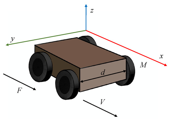
Figure 1. An unmanned ground vehicle system model.

Let the disturbance ${\delta }_k=\left[\begin{array}{c}0.05sin\left(k\right)+0.05\\ -0.05cos\left(k\right)+0.05\end{array}\right]$ and choose the nonlinear function $F(x_1,x_2)=\left[\begin{array}{c}0.05sin\left(x_1\right)\\ 0.05cos\left(x_2\right)\end{array}\right]$. Moreover, let $E=\left[\begin{array}{c}1\\ 0\end{array}\right]$ and for $\forall k\ge 0$, $f=0$, which in this case is fault-free. Then, select the coordinate transformation matrix H as

$$H=\left[\begin{array}{cc}1& -1\\ 1& -2\end{array}\right].$$

The remaining parameters are given below:

$$\lambda =0.01,\eta =0.01,\rho =3.$$

(40)

Then, the matrix $\widehat{F}$ and weighting matrix P are obtained as

$$\widehat{F}=\left[\begin{array}{cccc}0.1& 0& 0.05& 0\\ 0& 0.1& 0& 0.05\\ 0.05& 0& 0.1& 0\\ 0& 0.05& 0& 0.1\end{array}\right],P=\left[\begin{array}{cccc}8.6103& -4.0690& 0.0901& -0.0426\\ -4.0690& 1.9229& -0.0426& 0.0201\\ 0.0901& -0.0426& 8.6103& -4.0690\\ -0.0426& 0.0201& -4.0690& 1.9229\end{array}\right].$$

Therefore, according to Theorem 3, we can obtain the gain matrix L as follows:

$$L=\left[\begin{array}{c}0.5038\\ -0.05\end{array}\right].$$

Through simulation, we can obtain the results as follows. Figure 2 and Figure 3 separately depict the state trajectories and estimation of $x_1$ and $x_2$. Figure 4 and Figure 5 verify that the error system gradually stabilizes to a positive lower bound, which proves the effectiveness of this method. Figure 6 shows the situation without faults. For the area where $0\in [r^{-},r^{+}]$, this means that the estimated values are still within the upper and lower boundaries, while for the area where $0\notin [r^{-},r^{+}]$, this indicates that the actuator is faulty. Moreover, Figure 7 manifests the intervals and triggering instants of the event, which also illustrates that the Zeno behavior does not happen. In the figures, ‘u’ denotes the upper bound of the estimation and ‘l’ represents the lower bound of the estimation.

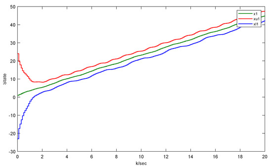
Figure 2. The original UGV system state $x_1$ and its interval estimates.

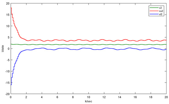
Figure 3. The original UGV system state $x_2$ and its interval estimates.

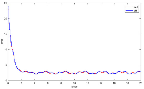
Figure 4. The UGV interval estimation error of $x_1$.

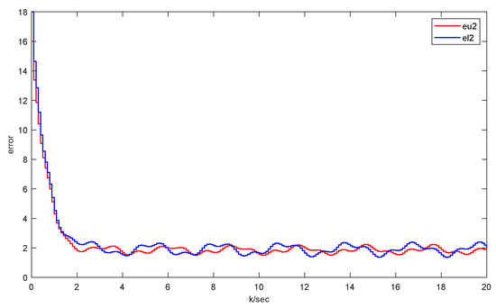
Figure 5. The UGV interval estimation error of $x_2$.

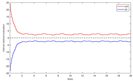
Figure 6. Detection residual of fault-free UGV case.

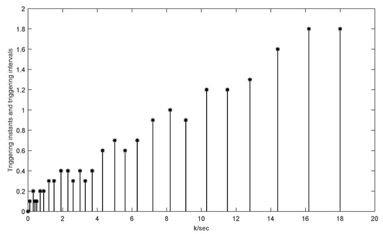
Figure 7. Triggering instants and intervals of the UGV system in 20 s.

4.1.2. Simulation with Random Faults

To validate the effectiveness of the developed results, we tested the situation where random faults exist. We used the same UGV model as above, with the actuator fault algorithm previously set as

$$f\left(k\right)=\left\{\begin{array}{ccc}{\left[\begin{array}{c}00\end{array}\right]}^T,\hfill & \hfill & 0\mathrm{s}<k\le 8\mathrm{s},\hfill \\ {\left[\begin{array}{c}2.51.2\end{array}\right]}^T,\hfill & \hfill & 8\mathrm{s}<k\le 13\mathrm{s},\hfill \\ {\left[\begin{array}{c}00\end{array}\right]}^T,\hfill & \hfill & 13\mathrm{s}<k\le 15\mathrm{s},\hfill \\ {\left[\begin{array}{c}2.01.5\end{array}\right]}^T,\hfill & \hfill & 15\mathrm{s}<k\le 20\mathrm{s}.\hfill \end{array}\right.$$

(41)

The residual results can be obtained in Figure 8 by simulation, and the following can be found:

$$\left\{\begin{array}{ccc}0\in [r^{-},r^{+}],\hfill & \hfill & 0\mathrm{s}<k<12.1\mathrm{s},\hfill \\ 0\notin [r^{-},r^{+}],\hfill & \hfill & 12.1\mathrm{s}\le k\le 13.5\mathrm{s},\hfill \\ 0\in [r^{-},r^{+}],\hfill & \hfill & 13.5\mathrm{s}<k<15.1\mathrm{s},\hfill \\ 0\notin [r^{-},r^{+}],\hfill & \hfill & 15.1\mathrm{s}\le k\le 20\mathrm{s}.\hfill \end{array}\right.$$

(42)

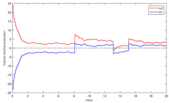
Figure 8. UGV detection residual at faults.

It is easy to see that the fault is detected in $0.1$ s, which proves the sensitivity and precision of the proposed method. Figure 9 shows the triggering intervals of the faulty cases, which also illustrates the characteristics of the proposed design for the fault detection DETIO in saving resources.

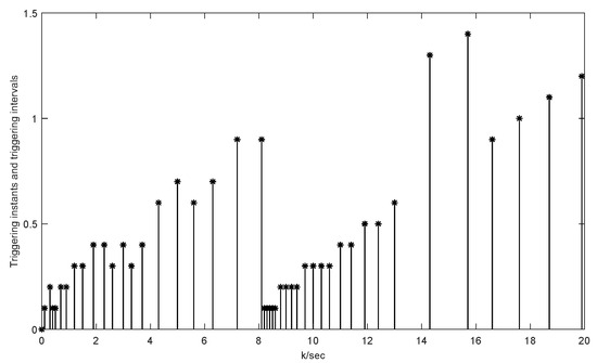
Figure 9. Triggering instants and intervals of the UGV system in 20 s under faults.

4.2. Example of an Unmanned Aerial Vehicle

4.2.1. Simulation of a Fault-Free Case

To further verify the applicability of the fault detection DETIO, we consider an unmanned aerial vehicle (UAV) model as shown in Figure 10. Referring to [29], the UAV system can be described as follows:

$$\left\{\begin{array}{c}\left[\begin{array}{c}\dot{\alpha }\left(t\right)\\ \dot{\beta }\left(t\right)\end{array}\right]=A\left[\begin{array}{c}\alpha \left(t\right)\\ \beta \left(t\right)\end{array}\right]+Bu\left(k\right)+p\left(k\right),\hfill \\ y\left(k\right)=C\left[\begin{array}{c}\alpha \left(t\right)\\ \beta \left(t\right)\end{array}\right].\hfill \end{array}\right.$$

(43)

where $\alpha \left(t\right)$ and $\beta \left(t\right)$ represent the angle of attack and the pitch rate of the UAV. $u\left(k\right)$ is the system input and $p\left(k\right)$ is the disturbance. $y\left(k\right)$ is the output of the UAV system. The partial parametric matrices are as follows:

$$A=\left[\begin{array}{cc}0.8825& 0.0987\\ -0.8458& 0.9122\end{array}\right],B=\left[\begin{array}{c}-0.0194\\ -1.9290\end{array}\right],$$

$$C=\left[\begin{array}{c}10.2\end{array}\right],D=\left[\begin{array}{c}10\\ 01\end{array}\right],E=\left[\begin{array}{c}2\\ 0\end{array}\right].$$

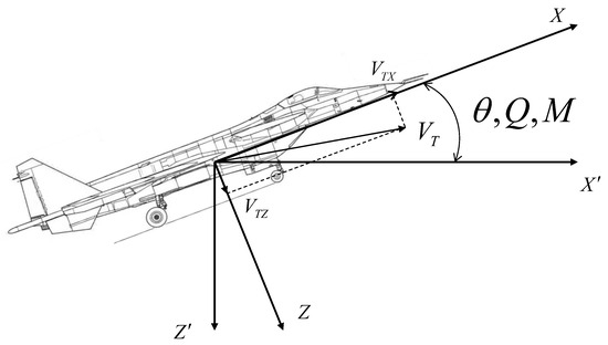
Figure 10. An unmanned aerial vehicle system model.

The external disturbance ${\delta }_k=\left[\begin{array}{c}0.1+0.1sin\left(k\right)\\ 0.1-0.1cos\left(k\right)\end{array}\right]$ and the nonlinear function $F(x_1,x_2)=\left[\begin{array}{c}0.1sin\left(x_1\right)\\ 0.1cos\left(x_2\right)\end{array}\right]$. Moreover, the transformation matrix H is selected as

$$H=\left[\begin{array}{cc}1& 0\\ -1& -2\end{array}\right].$$

The remaining parameters remain consistent with the parameters in (40), and for $\forall k\ge 0$, $f=0$. Then, the matrix $\widehat{F}$ and the weighting matrix P are obtained as

$$\widehat{F}=\left[\begin{array}{cccc}0.1& 0& 0.05& 0\\ 0& 0.1& 0& 0.05\\ 0.05& 0& 0.1& 0\\ 0& 0.05& 0& 0.1\end{array}\right],P=\left[\begin{array}{cccc}23.3435& -0.9440& -0.1006& 0.0041\\ -0.9440& 0.0382& 0.0041& -0.0002\\ -0.1006& 0.0041& 23.3435& -0.9440\\ 0.0041& -0.0002& -0.9440& 0.0382\end{array}\right].$$

Through Theorem 3, we can obtain the gain matrix of the UAV system as follows:

$$L=\left[\begin{array}{c}0.8687\\ -0.85\end{array}\right].$$

The following are the results of the simulation. Figure 11 and Figure 12 manifest the original states and its interval estimations. Figure 13 and Figure 14 illustrate the effectiveness of this approach in the UAV model. Figure 15 shows the residual which proves that no faults are detected in this fault-free situation. And Figure 16 displays the intervals and triggering instants of the event with no occurrence of Zeno behavior.

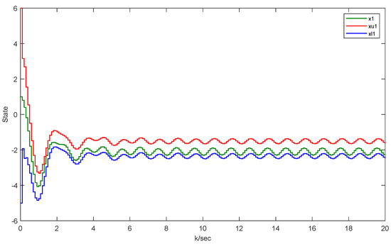
Figure 11. The original UAV system state $x_1$ and its interval estimates.

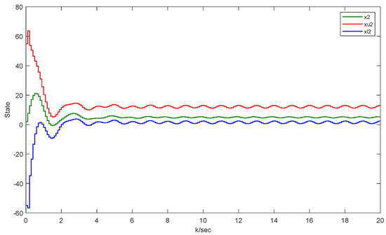
Figure 12. The original UAV system state $x_2$ and its interval estimates.

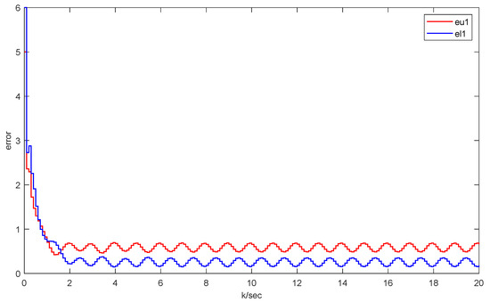
Figure 13. The UAV interval estimation error of $x_1$.

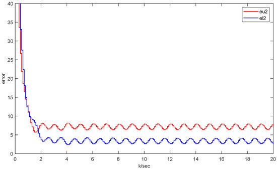
Figure 14. The UAV interval estimation error of $x_2$.

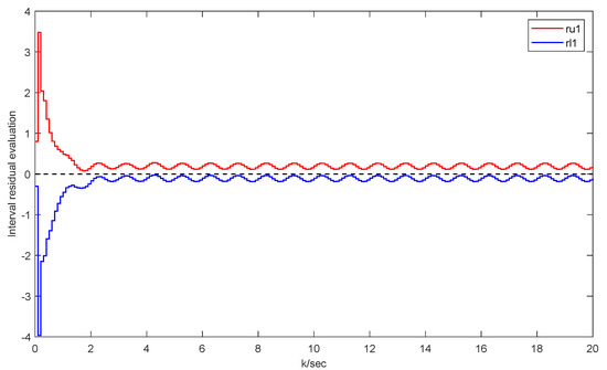
Figure 15. Detection residual of the fault-free UAV case.

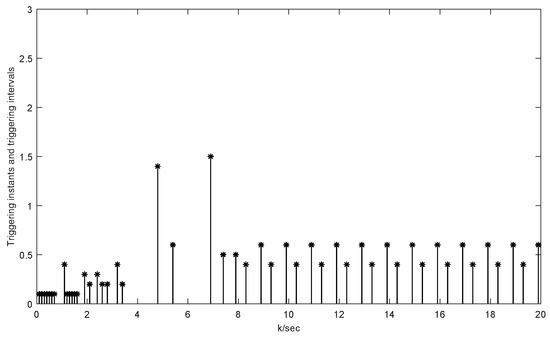
Figure 16. Triggering instants and intervals of UAV system in 20 s.

4.2.2. Simulation with Random Faults

To verify the effectiveness and applicability of this approach, random faults are introduced into the above UAV model, and the fault algorithm is preset as follows:

$$f\left(k\right)=\left\{\begin{array}{ccc}{\left[\begin{array}{c}00\end{array}\right]}^T,\hfill & \hfill & 0\mathrm{s}<k\le 6\mathrm{s},\hfill \\ {\left[\begin{array}{c}-1.0-0.7\end{array}\right]}^T,\hfill & \hfill & 6\mathrm{s}<k\le 15\mathrm{s},\hfill \\ {\left[\begin{array}{c}00\end{array}\right]}^T,\hfill & \hfill & 15\mathrm{s}<k\le 20\mathrm{s}.\hfill \end{array}\right.$$

(44)

Through simulation, we can obtain the results shown in Figure 17, where we can find that

$$\left\{\begin{array}{ccc}0\in [r^{-},r^{+}],\hfill & \hfill & 0\mathrm{s}<k<6.6\mathrm{s},\hfill \\ 0\notin [r^{-},r^{+}],\hfill & \hfill & 6.6\mathrm{s}\le k\le 16.5\mathrm{s},\hfill \\ 0\in [r^{-},r^{+}],\hfill & \hfill & 16.5\mathrm{s}<k<20\mathrm{s}.\hfill \end{array}\right.$$

(45)

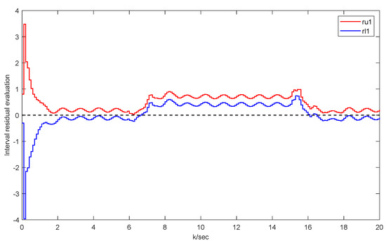
Figure 17. UAV detection residual at faults.

This indicates the occurrence of the faults in the system. Figure 18 exhibits the triggering intervals of the UAV example under faults, demonstrating the economical feature of saving system resources using this approach.

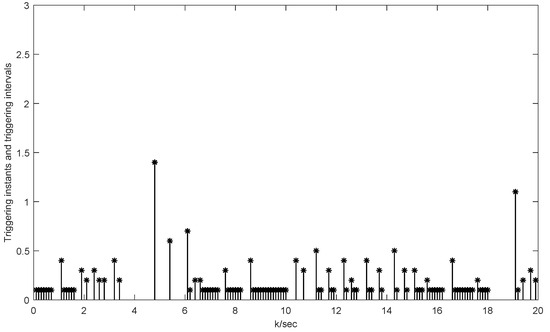
Figure 18. Triggering instants and intervals of UAV system in 20 s under faults.

4.3. Quantitative Comparison with UGV Model

Consider the UGV model mentioned in Section 4.1, to further demonstrate the proposed method of this article, a comparison is conducted between our approach and the fault detection with ETIO using static ETM. Figure 19 shows the triggering instants and intervals of static ETIO fault detection under random faults in (41). Table 1 displays the event-triggered counts of the proposed method, the static ETIO approach, and the traditional IO technique, respectively.

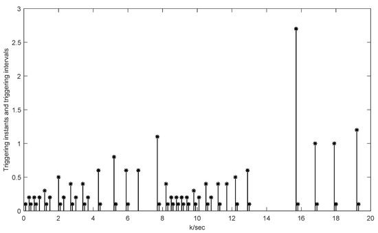
Figure 19. Triggering instants and intervals of the UGV system by ETIO in 20 s under faults.

Table 1. The number of event-triggered instants of different fault detection methods.

Methods	Number of Event-Triggered Instants
DETIO Fault Detection	44 Times
Static ETIO Fault Detection	58 Times
Traditional IO Fault Detection 1	200 Times

¹ Fundamental sample time is set to 0.1 s.

From Table 1, we can conclude that the proposed method of this paper has a better performance in resource saving and data transmission, compared to other methods without DETM.

5. Conclusions

This paper studies a DETIO-based fault detection approach that is applied to nonlinear CPSs. A DETIO framework is designed through the positive system theory and integrated DETM to minimize data transmission and conserve network resources. For systems which violate the non-negative condition, the coordinate transformation method is introduced to enhance the flexibility of designing the observer. Finally, numerical simulations of two situations are manifested to demonstrate the viability of the developed approach. Based on both a simplified UGV model and a UAV model, the interval estimation of states is obtained by fault-free cases. Then, through simulation with random faults, we prove the effectiveness and rapidity of the presented method. Furthermore, the avoidance of Zeno behavior is also illustrated by the simulation, which proves the effectiveness in conserving resources. Moreover, three different fault detection approaches based on the UGV model are compared to verify the superiority of the proposed method. In future work, we will investigate the deployment of DETM in interval observer-based fault detection of distributed CPSs.

References

- Poovendran, R.; Sampigethaya, K.; Gupta, S.K.S.; Lee, I.; Prasad, K.V.; Corman, D.; Paunicka, J.L. Special Issue on Cyber—Physical Systems. Proc. IEEE 2012, 100, 6–12. [Google Scholar] [CrossRef]
- Oyewole, P.A.; Jayaweera, D. Power System Security with Cyber-Physical Power System Operation. IEEE Access 2020, 8, 179970–179982. [Google Scholar] [CrossRef]
- Dionysios, N.; Christos, M. Stress-testing water distribution networks for cyber-physical attacks on water quality. Urban Water J. 2022, 19, 256–270. [Google Scholar]
- Lu, A.Y.; Yang, G.H. Secure Switched Observers for Cyber-Physical Systems Under Sparse Sensor Attacks: A Set Cover Approach. IEEE Trans. Autom. Control 2019, 64, 3949–3955. [Google Scholar] [CrossRef]
- Ye, L.; Zhu, F.; Zhang, J. Sensor attack detection and isolation based on sliding mode observer for cyber-physical systems. Int. J. Adapt. Control Signal Process. 2020, 34, 469–483. [Google Scholar] [CrossRef]
- Hu, L.; Wang, Z.; Han, Q.L.; Liu, X. State estimation under false data injection attacks: Security analysis and system protection. Automatica 2018, 87, 176–183. [Google Scholar] [CrossRef]
- Qin, Y.; Huang, J.; Wu, H. An Interval Observer for a Class of Cyber–Physical Systems with Disturbance. Axioms 2024, 13, 18. [Google Scholar] [CrossRef]
- Zhang, J.; Huang, J.; Li, C. Distributed Interval Observers with Switching Topology Design for Cyber-Physical Systems. Mathematics 2024, 12, 163. [Google Scholar] [CrossRef]
- Heemels, W.P.M.H.; Donkers, M.C.F.; Teel, A.R. Periodic Event-Triggered Control for Linear Systems. IEEE Trans. Autom. Control 2013, 58, 847–861. [Google Scholar] [CrossRef]
- Yang, X.; Huang, M.; Wu, Y.; Tan, X. A Proportional–Integral Observer-Based Dynamic Event-Triggered Consensus Protocol for Nonlinear Positive Multi-Agent Systems. Axioms 2024, 13, 384. [Google Scholar] [CrossRef]
- Shi, D.; Chen, T.; Shi, L. Event-triggered maximum likelihood state estimation. Automatica 2014, 50, 247–254. [Google Scholar] [CrossRef]
- Deng, C.; Che, W.W.; Wu, Z.G. A Dynamic Periodic Event-Triggered Approach to Consensus of Heterogeneous Linear Multiagent Systems with Time-Varying Communication Delays. IEEE Trans. Cybern. 2021, 51, 1812–1821. [Google Scholar] [CrossRef] [PubMed]
- Zhang, M.; Zhang, J.; Huang, J. Design of dynamic event-triggered interval observer for Euler-lagrange systems under stealthy attack. In Circuits, Systems, and Signal Processing; Springer: Berlin/Heidelberg, Germany, 2025; pp. 1–24. [Google Scholar]
- Huong, D.C.; Huynh, V.T.; Trinh, H. Design of event-triggered interval functional observers for systems with input and output disturbances. Math. Methods Appl. Sci. 2021, 44, 13968–13978. [Google Scholar] [CrossRef]
- Fei, Z.; Yang, L.; Guan, C.; Wu, Y. Zonotopic state bounding for 2-D systems with dynamic event-triggered mechanism. Automatica 2023, 154, 111066. [Google Scholar] [CrossRef]
- Guo, S.; Tang, M.; Huang, D.; Song, J. State estimation and finite-frequency fault detection for interconnected switched cyber-physical systems. Sci. China Inf. Sci. 2023, 66, 192204. [Google Scholar] [CrossRef]
- Corradini, M.L.; Cristofaro, A. Robust detection and reconstruction of state and sensor attacks for cyber-physical systems using sliding modes. IET Control Theory Appl. 2017, 11, 1756–1766. [Google Scholar] [CrossRef]
- Jiang, W.; Wen, L.; Zhan, J.; Jiang, K. Design optimization of confidentiality-critical cyber physical systems with fault detection. J. Syst. Archit. 2020, 107, 101739. [Google Scholar] [CrossRef]
- He, Y.; Nie, B.; Zhang, J.; Kumar, P.M.; Muthu, B.A. Fault Detection and Diagnosis of Cyber-Physical System Using the Computer Vision and Image Processing. Wirel. Pers. Commun. 2022, 127, 2141–2160. [Google Scholar] [CrossRef]
- Jafari, N.; Lopes, A.M. Fault Detection and Identification with Kernel Principal Component Analysis and Long Short-Term Memory Artificial Neural Network Combined Method. Axioms 2023, 12, 583. [Google Scholar] [CrossRef]
- Wilhelm, Y.; Reimann, P.; Gauchel, W.; Mitschang, B. Overview on hybrid approaches to fault detection and diagnosis: Combining data-driven, physics-based and knowledge-based models. Procedia CIRP 2021, 99, 278–283. [Google Scholar] [CrossRef]
- Liu, Q.; Long, Y.; Li, T.; Chen, C.L.P. Attack Tolerant Fault Detection for CPSs: An Unknown Input Interval Observer Approach. IEEE Trans. Autom. Sci. Eng. 2025, 22, 1163–1172. [Google Scholar] [CrossRef]
- Zhu, F.; Tang, Y.; Wang, Z. Interval-Observer-Based Fault Detection and Isolation Design for T-S Fuzzy System Based on Zonotope Analysis. IEEE Trans. Fuzzy Syst. 2022, 30, 945–955. [Google Scholar] [CrossRef]
- Zhang, K.; Jiang, B.; Yan, X.G.; Mao, Z. Incipient Fault Detection for Traction Motors of High-Speed Railways Using an Interval Sliding Mode Observer. IEEE Trans. Intell. Transp. Syst. 2019, 20, 2703–2714. [Google Scholar] [CrossRef]
- Yin, Z.; Huang, J.; Zhang, Y. Event-triggered interval observer design for a class of Euler-Lagrange systems with disturbances. Trans. Inst. Meas. Control 2023. [Google Scholar] [CrossRef]
- Efimov, D.; Raïssi, T.; Zolghadri, A. Control of nonlinear and LPV systems: Interval observer-based framework. IEEE Trans. Autom. Control 2013, 58, 773–778. [Google Scholar] [CrossRef]
- Guo, S.; Zhu, F. Interval observer design for discrete-time switched system. IFAC-PapersOnLine 2017, 50, 5073–5078. [Google Scholar] [CrossRef]
- Huang, J.; Fan, J.; Dinh, T.N.; Zhao, X.; Zhang, Y. Event-triggered interval estimation method for cyber–Physical systems with unknown inputs. ISA Trans. 2022, 135, 1–12. [Google Scholar] [CrossRef]
- Zhang, C.L.; Yang, G.H.; Lu, A.Y. Resilient observer-based control for cyber-physical systems under denial-of-service attacks. Inf. Sci. 2021, 545, 102–117. [Google Scholar] [CrossRef]
Disclaimer/Publisher’s Note: The statements, opinions and data contained in all publications are solely those of the individual author(s) and contributor(s) and not of MDPI and/or the editor(s). MDPI and/or the editor(s) disclaim responsibility for any injury to people or property resulting from any ideas, methods, instructions or products referred to in the content. |
© 2025 by the authors. Licensee MDPI, Basel, Switzerland. This article is an open access article distributed under the terms and conditions of the Creative Commons Attribution (CC BY) license (https://creativecommons.org/licenses/by/4.0/).