Dynamics of HLB Transmission: Integrating Saturated Removal and Vector Bias in Spatial/Non-Spatial Models

Abstract

Huanglongbing (HLB), a globally devastating citrus disease, demands sophisticated mathematical modeling to decipher its complex transmission dynamics and inform optimized disease management protocols. This investigation develops an innovative compartmental framework that simultaneously incorporates two critical factors in HLB epidemiology: saturated removal rates of infected citrus trees and behavioral bias in vector movement patterns. Our study delves into the dynamics of non-spatial systems by analyzing the basic reproduction numbers, equilibria, bifurcation phenomena, and the stability of these equilibria. Additionally, we explore the impact of spatial factors on system stability. Results indicate that when the basic reproduction number $R_0<1$, the system may exhibit bistable behavior, while $R_0>1$ leads to a unique stable equilibrium. Notably, vector bias significantly enhances the likelihood of forward bifurcation, and the delay in the removal of diseased trees increases the risk of backward bifurcation. However, reaction–diffusion processes do not alter the stability of the system’s equilibria, and the spatial system lacks complex dynamic properties. This research offers valuable insights into the mechanisms driving HLB transmission and provides a foundation for developing effective control strategies.

1. Introduction

Huanglongbing (HLB), formerly termed citrus greening disease, is a devastating and highly contagious plant pathology caused by Candidatus Liberibacter species. This pathogen inflicts systemic damage to citrus phloem tissues, manifesting as severe chlorosis, fruit deformities, and premature abscission, ultimately leading to catastrophic declines in both yield and fruit quality. Since its initial detection in China, HLB has emerged as a persistent biosecurity threat, inflicting substantial economic losses across global citrus-producing regions [1]. Despite decades of research, effective curative measures remain elusive, cementing HLB’s status as one of the most intractable challenges in contemporary phytopathology.

The Asian citrus psyllid (Diaphorina citri), a hemipteran insect within the Psyllidae family, serves as the sole natural vector for HLB transmission [2]. This oligophagous pest preferentially colonizes Rutaceae hosts, including citrus (Citrus spp.), orange jasmine (Murraya paniculata), and Chinese boxthorn (Lycium chinense), with feeding activities concentrated on emerging flush growth. Intriguingly, Mann et al. [3] demonstrated that HLB-infected plants undergo transcriptomic reprogramming, resulting in altered volatile organic compound profiles and visual cues (e.g., leaf yellowing). These pathogen-induced modifications enhance host attractiveness to D. citri, thereby creating a positive feedback loop that amplifies vector recruitment and oviposition on infected hosts.

Current HLB management strategies rely heavily on the prompt elimination of symptomatic trees. Although linear removal rate functions have been conventionally employed in epidemiological models [4,5,6], such approaches inadequately capture real-world operational constraints. Drawing inspiration from [7]’s saturation-dependent therapeutic framework, this study introduces a nonlinear removal function,

$$M\left(I_h\right)={\displaystyle \frac{\delta I_h}{1+\alpha I_h}},$$

where $\delta$ denotes the baseline removal rate and $\alpha$ quantifies delayed intervention effects. This formulation reflects two critical regimes: (1) at low infection intensities, removal approximates linear dynamics ($M\left(I_h\right)\approx \delta I_h$); (2) at large infection scales, removal plateaus at $\delta /\alpha$, mirroring saturation effects from finite resources (e.g., labor shortages, budgetary limitations). Notably, setting $\alpha =0$ recovers the classical linear model, enabling direct comparison with prior studies.

Spatiotemporal heterogeneity constitutes a pivotal yet underexplored dimension in HLB epidemiology. Although temporal models dominate the literature [8,9], the spatial dispersal capacity of D. citri, particularly adult psyllids’ ability to traverse kilometers via wind-aided flight, demands integration of diffusion dynamics. Orchards rarely exist as isolated systems; rather, pathogen–vector interactions operate across interconnected agricultural landscapes where microclimatic variations and anthropogenic activities modulate transmission thresholds. A spatially explicit modeling framework thus offers critical insights into how geographic disparities in resource allocation, surveillance efficacy, and vector mobility influence epidemic trajectories.

The dissemination of diseases is affected by both temporal and spatial factors. As a result, the spatial aspect of infectious disease models has attracted substantial interest. This focus has led to remarkable outcomes in epidemiology and ecology, and these models have been successfully applied in practical disease prevention and control measures [8,9]. Given that the Asian citrus psyllid has a certain flight capacity, adult psyllids are capable of dispersing between orchards through near-ground strong winds. Developing an HLB transmission model that incorporates spatial diffusion terms can more accurately represent the influence of spatial heterogeneity on disease spread.

This paper is structured as follows: Section 2 formulates a non-spatial compartmental model incorporating infected-tree removal and vector preference dynamics. Section 3 rigorously analyzes system equilibria, derives the basic reproduction number ($R_0$), establishes global stability criteria, and examines bifurcation behavior at $R_0=1$. Section 4 extends the model through diffusion operators to investigate pattern formation and Turing instability in spatial systems. Section 5 validates theoretical predictions via numerical simulations, and Section 6 synthesizes key findings and their implications for integrated pest management.

2. Model Formulation

Based on compartment modeling principles, we classify citrus trees into two epidemiological states: susceptible ($S_h$) and infected ($I_h$). Similarly, the psyllid vector population is partitioned into susceptible ($S_v$) and infected ($I_v$) categories. $N_h\left(t\right)$ denotes the total number of citrus trees in the orchard at time t, such that $N_h\left(t\right)=S_h\left(t\right)+I_h\left(t\right)$. Likewise, $N_v\left(t\right)$ denotes the total number of psyllids in the orchard at time t, with $N_v\left(t\right)=S_v\left(t\right)+I_v\left(t\right)$.

A critical behavioral factor in HLB transmission is the preferential feeding tendency of psyllids toward infected citrus trees. Field observations suggest that infected trees emit distinct volatile organic compounds (VOCs) which act as olfactory cues, attracting adult psyllids to settle and feed more frequently on $I_h$ hosts compared to $S_h$ hosts. To quantify this behavior, we introduce w as the preference coefficient, defined as the ratio of psyllid visitation probability to infected versus susceptible trees. Specifically, if $w>1$, psyllids exhibit a stronger attraction to infected trees; if $w<1$, psyllids avoid infected trees, and if $w=1$, no preference exists (equal visitation rates). Building on the known tropic behavior of psyllids, this paper assumes $w>1$. Consequently, the force of infection for citrus trees is modulated by w, such that the effective contact rate between infected psyllids ($I_v$) and susceptible trees ($S_h$) follows a standard style:

$${\beta }_h{\displaystyle \frac{S_h}{S_h+w{I}_h}},$$

where ${\beta }_h$ is the transmission rate between infected psyllids and susceptible citrus trees. Similarly, the force of infection for psyllids is

$${\beta }_v{\displaystyle \frac{S_v}{S_h+w{I}_h}},$$

where ${\beta }_v$ is the transmission rate between susceptible psyllids and infected citrus trees.

Considering the operational constraints imposed by limited human resources and economic capacities in agricultural management, we reasonably assume that disease containment measures exhibit a saturation effect when dealing with large-scale infections. This motivates the adoption of a saturated removal rate formulated as

$${\displaystyle \frac{\delta I_h}{1+\alpha I_h}},$$

where $\delta$ represents the maximum theoretical removal rate under ideal resource conditions and $\alpha$ quantifies the delayed response intensity caused by logistical constraints, with larger $\alpha$ values indicating stronger suppression of removal efficiency at high infection levels. The denominator term ($1+\alpha I_h$) introduces a density-dependent inhibition mechanism, reflecting the reality that removal efficiency decreases proportionally as infected citrus tree density ($I_h$) increases. This aligns with Michaelis–Menten-type saturation kinetics observed in biological systems [10].

Further, we assume that the orchardist employs an “immediate replanting” strategy, thereby maintaining a constant total number of citrus trees, denoted by K. Based on the above assumptions, we establish a HLB transmission model with saturated removal rates and psyllid bias:

$$\left\{\begin{array}{c}{\displaystyle \frac{d{S}_h}{dt}}=d{I}_h+{\displaystyle \frac{\delta I_h}{1+\alpha I_h}}-{\beta }_h{\displaystyle \frac{S_h}{S_h+w{I}_h}}{I}_v,\hfill \\ {\displaystyle \frac{d{I}_h}{dt}}={\beta }_h{\displaystyle \frac{S_h}{S_h+w{I}_h}}{I}_v-d{I}_h-{\displaystyle \frac{\delta I_h}{1+\alpha I_h}},\hfill \\ {\displaystyle \frac{d{S}_v}{dt}}=\Lambda -{\beta }_v{\displaystyle \frac{w{I}_h}{S_h+w{I}_h}}{S}_v-u{S}_v,\hfill \\ {\displaystyle \frac{d{I}_v}{dt}}={\beta }_v{\displaystyle \frac{w{I}_h}{S_h+w{I}_h}}{S}_v-u{I}_v,\hfill \end{array}\right.$$

(1)

where d is the natural mortality rate of citrus trees, $\Lambda$ is the constant recruitment rate of psyllids and u is the mortality rate of psyllids, including natural mortality and mortality caused by pesticide spraying. We also assume that all parameters of the model are positive.

Given that the life cycle of citrus psyllids is significantly shorter than that of citrus trees, the psyllid-related subsystem will swiftly converge toward an equilibrium state. Consequently, the dynamic characteristics of system (1) can be simplified by analyzing its limiting system. It follows from system (1) that $N_h\left(t\right)=K$ for all $t\ge 0$, and ${lim}_{t\to \infty }{N}_v\left(t\right)={\displaystyle \frac{\Lambda }{u}}$. Thus, the limit system of system (1) yields

$$\left\{\begin{array}{c}{\displaystyle \frac{d{I}_h}{dt}}={\beta }_h{\displaystyle \frac{(K-I_h)}{(K-I_h)+w{I}_h}}{I}_v-d{I}_h-{\displaystyle \frac{\delta I_h}{1+\alpha I_h}},\hfill \\ {\displaystyle \frac{d{I}_v}{dt}}={\beta }_v{\displaystyle \frac{w{I}_h}{(K-I_h)+w{I}_h}}({\displaystyle \frac{\Lambda }{u}}-I_v)-u{I}_v.\hfill \end{array}\right.$$

(2)

The flowchart depicting the transmission dynamics of citrus HLB is presented in Figure 1. The parameters and their biological significance in model (2) are summarized in Table 1.

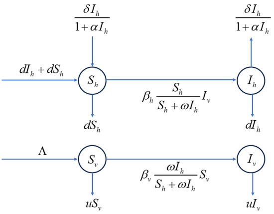
Figure 1. Flowchart of citrus HLB transmission.

Table 1. Parameter description.

Parameters	Description
${\beta }_h$	Infection rate between infected psyllids and susceptible citrus trees
w	Preference parameter of psyllids for infected citrus trees
d	Natural mortality of citrus trees
$\delta$	maximum theoretical removal rate of infected citrus trees
$\alpha$	The extent of the delayed effect for treatment
$\Lambda$	Constant recruitment rate of psyllids
${\beta }_v$	Infection rate between susceptible psyllids and infected citrus trees
u	Mortality of psyllids
K	Total number of citrus trees in the orchard

Define

$$\Omega =\left\{(I_h,I_v)\in R_{+}^2:0\le I_h\le K,0\le I_v\le {\displaystyle \frac{\Lambda }{u}}\right\}.$$

It is evident that $\Omega$ is the positively invariant set of system (2).

3. Stability and Bifurcation Analysis for Non-Spatial System (2)

In the following, we aim to systematically investigate the dynamic behavior of system (2). We first establish the fundamental epidemiological threshold by deriving the basic reproduction number $R_0$ by using the next-generation matrix analysis.

3.1. Basic Reproduction Number

In this subsection, we employ the next-generation matrix method (see Van den Driessche and Watmough [11]) to determine the basic reproduction number $R_0$ of system (2).

Let $x={(I_h,I_v)}^T$. Then, model (2) can be rewritten as

$${\displaystyle \frac{dx}{dt}}=\mathcal{F}\left(x\right)-\mathcal{V}\left(x\right),$$

where

$$\begin{array}{c}\mathcal{F}\left(x\right)=\left(\begin{array}{c}{\beta }_h{\displaystyle \frac{(K-I_h)}{(K-I_h)+w{I}_h}}{I}_v\\ {\beta }_v{\displaystyle \frac{w{I}_h}{(K-I_h)+w{I}_h}}({\displaystyle \frac{\Lambda }{u}}-I_v)\end{array}\right),\mathcal{V}\left(x\right)=\left(\begin{array}{c}d{I}_h+{\displaystyle \frac{\delta I_h}{1+\alpha I_h}}\\ u{I}_v\end{array}\right).\end{array}$$

Here, the function $\mathcal{F}\left(x\right)$ represents the rate of new infections, while $\mathcal{V}\left(x\right)$ describes the net transition rate between compartments. Following the next-generation matrix framework [11], we derive the infection matrix F and the transition matrix V as

$$\begin{array}{c}F=\left(\begin{array}{cc}0& {\beta }_h\\ {\displaystyle \frac{{\beta }_v\Lambda w}{uK}}& 0\end{array}\right),V=\left(\begin{array}{cc}d+\delta & 0\\ 0& u\end{array}\right).\end{array}$$

The next-generation matrix $F{V}^{-1}$ governs the reproduction dynamics of system (2). By computing its spectral radius $\rho \left(F{V}^{-1}\right)$, we yield

$$\rho \left(F{V}^{-1}\right)=\sqrt{{\displaystyle \frac{{\beta }_h{\beta }_v\frac{\Lambda }{u}w}{(d+\delta )uK}}}.$$

According to Theorem 2 in [11], the basic reproduction number for system (2) is therefore defined as

$$R_0=\sqrt{{\displaystyle \frac{{\beta }_h{\beta }_v\frac{\Lambda }{u}w}{(d+\delta )uK}}}.$$

3.2. Existence of Equilibria

It is clear that system (2) always has a disease-free equilibrium $E_0=(I_h,I_v)=(0,0)$. Next, we investigate the existence of the endemic equilibrium $E^{\ast }=(I_h^{\ast },I_v^{\ast })$ in the feasible region $\Omega$, where $I_h^{\ast }>0$ and $I_v^{\ast }>0$, and we satisfy the following equation:

$$\begin{array}{cc}& {\displaystyle \frac{{\beta }_h\left(K-I_h^{\ast }\right)I_v^{\ast }}{\left(K-I_h^{\ast }\right)+w{I}_h^{\ast }}}-d{I}_h^{\ast }-{\displaystyle \frac{\delta I_h^{\ast }}{1+\alpha I_h^{\ast }}}=0,\hfill \\ & {\displaystyle \frac{{\beta }_v\left(\frac{\Lambda }{u}-I_v^{\ast }\right)w{I}_h^{\ast }}{\left(K-I_h^{\ast }\right)+w{I}_h^{\ast }}}-u{I}_v^{\ast }=0.\hfill \end{array}$$

By combining and rearranging these two equations, we determine that $I_h^{\ast }$ must be the positive root of the following characteristic equation:

$$f\left(I_h\right)=A_3{I}_h^3+A_2{I}_h^2+A_1{I}_h+A_0=0,$$

(3)

where

$$\begin{array}{cc}& A_3=\alpha d(w-1)({\beta }_{v}w+u(w-1)),\hfill \\ & A_2={\beta }_h{\beta }_v{\displaystyle \frac{\Lambda }{u}}\alpha w+\alpha dK\left({\beta }_{v}w+2u(w-1)\right)+(d+\delta )(w-1)({\beta }_{v}w+u(w-1)),\hfill \\ & A_1=K(d+\delta )\left({\beta }_{v}w+2u(w-1)\right)+u{K}^2\alpha d-{\beta }_h{\beta }_v{\displaystyle \frac{\Lambda }{u}}w(\alpha K-1),\hfill \\ & A_0=u{K}^2(d+\delta )-{\beta }_h{\beta }_v{\displaystyle \frac{\Lambda }{u}}Kw=(d+\delta )K^{2}u(1-R_0^2).\hfill \end{array}$$

Theorem 1.

System (2) has at least one endemic equilibrium if $R_0>1$.

Proof of Theorem 1. 

The existence of the endemic equilibrium of the system (2) depends on the positive roots of the characteristic Equation (3). Since $A_3>0$, we have ${lim}_{I_h\to \infty }f\left(I_h\right)=\infty$. If $R_0>1$, then $f\left(0\right)=A_0<0$. Therefore, Equation (3) has at least one positive root. In other words, system (2) always has an endemic equilibrium whenever $R_0>1$. □

Next, we use Descartes’ rule of signs to determine the number of positive roots of Equation (3) when $R_0<1$.

As shown in Table 2, when $R_0<1$, system (2) may have endemic equilibria. To further analyze this, we aim to determine a condition that guarantees the existence of an endemic equilibrium when $R_0<1$. This condition is indicated by the sign of ${\displaystyle \frac{\partial I_h}{\partial R_0}}$ being negative when $I_h=0,R_0=1$. If this condition is satisfied, system (2) exhibits two endemic equilibria when $R_0<1$. Otherwise, no endemic equilibrium exists.

Table 2. Number of possible positive roots of Equation (3).

Case	${\mathit{A}}_3$	${\mathit{A}}_2$	${\mathit{A}}_1$	${\mathit{A}}_0$	${\mathit{R}}_0$	Possible Number of Positive Roots
1	+	+	+	-	$R_0>1$	one
2	+	+	-	-	$R_0>1$	one
3	+	+	+	+	$R_0<1$	zero
4	+	+	−	+	$R_0<1$	two or zero

To achieve this, we first modify $A_i$ in $f\left(I_h\right)$ for $i=0,1,2,3$ to express it as a function of $R_0$. This is completed by setting

$${\beta }_h^{★}={\displaystyle \frac{(d+\delta )uK{R}_0^2}{{\beta }_v\frac{\Lambda }{u}w}}.$$

Substituting ${\beta }_h={\beta }_h^{★}$ into $A_0,A_1,A_2$, and $A_3$, and then taking the partial derivative of $I_h$ with respect to $R_0$ from $f\left(I_h\right)$ and evaluating it in $R_0=1,I_h=0$, yields the following:

$${\left.{\displaystyle \frac{\partial I_h}{\partial R_0}}\right|}_{I_h=0,R_0=1}={\left.{\displaystyle \frac{-\frac{\partial A_0}{\partial R_0}}{A_1\left(R_0\right)}}\right|}_{I_h=0,R_0=1},$$

where

$${\left.{\displaystyle \frac{\partial A_0}{\partial R_0}}\right|}_{I_h=0,R_0=1}=-2(d+\delta )K^{2}u.$$

Since ${\displaystyle \frac{\partial A_0}{\partial R_0}}<0$, the condition ${\displaystyle \frac{\partial I_h}{\partial R_0}}<0$ holds if and only if $A_1\left(R_0\right)<0$. This is equivalent to

$$\alpha >{\alpha }^{\ast }\doteq {\displaystyle \frac{(d+\delta )({\beta }_{v}w+2wu-u)}{uK\delta }}.$$

(4)

These results lead to the following theorem.

Theorem 2.

When $R_0<1$, system (2) has two endemic equilibria in an interval provided that

$$\alpha >{\alpha }^{\ast }={\displaystyle \frac{(d+\delta )({\beta }_{v}w+2wu-u)}{uK\delta }}.$$

To further confirm the existence interval of the endemic equilibrium, we define

$${▵}_{R_0}=B^2-4AC,$$

where $A=A_2^2-3A_1{A}_3$, $B=A_1{A}_2-9A_0{A}_3$, $C=A_1^2-3A_0{A}_2$, and $A_0,A_1,A_2,A_3$ are determined by Equation (3).

Let ${▵}_{R_0}=0$, solve the equation about $R_0$, and get

$$R_0^c=\sqrt{{\displaystyle \frac{27A_3^2{K}^{2}u(d+\delta )-9A_1{A}_2{A}_3+2A_2^3-2\sqrt{27{\left(A_1{A}_2{A}_3\right)}^2-27A_1^3{A}_3^3-9A_1{A}_2^4{A}_3+A_2^6}}{27A_3^{2}u(d+\delta )K^2}}}⩾0.$$

Therefore, we can obtain the following results more precisely.

Theorem 3.

Suppose $\alpha >{\alpha }^{\ast }$, then the following conclusions are valid:

(1) When $R_0^c<R_0<1$, system (2) has two distinct endemic equilibria, which are denoted by $E_1={(I_{h1},I_{v1})}^T$ and $E_2={(I_{h2},I_{v2})}^T$.

(2) When $R_0=R_0^c<1$, two endemic equilibria $E_1$ and $E_2$ coalesce into $\overline{E}={(\overline{I_h},\overline{I_v})}^T$.

(3) When $R_0<R_0^c<1$, system (2) has no endemic equilibrium.

3.3. Stability of the Equilibrium

Theorem 4.

For system (2), $E_0$ is locally asymptotically stable when $R_0<1$, and it becomes unstable when $R_0>1$. Moreover, when $R_0<1$, $E_0$ is globally asymptotically stable in the region Ω when it has a unique equilibrium.

Proof of Theorem 4. 

First, we prove the local stability of the disease-free equilibrium $E_0$. The Jacobian matrix of system (2) at $E_0$ is

$$\begin{array}{c}\hfill J\left(E_0\right)=\left(\begin{array}{cc}-d-\delta & {\beta }_h\\ {\displaystyle \frac{{\beta }_v\Lambda w}{uK}}& -u\end{array}\right).\end{array}$$

The characteristic equation associated with $E_0$ is

$${\lambda }^2+a_1\lambda +a_2=0,$$

(5)

where $a_1=u+d+\delta$, $a_2=u(d+\delta )\left(1-R_0^2\right)$.

Obviously, $a_1>0$, and $a_2=u(d+\delta )\left(1-R_0^2\right)>0$, provided that $R_0<1$. According to Routh–Hurwitz criterion, $E_0$ is locally asymptotically stable provided that $R_0<1$. If $R_0>1$, then $a_2<0$, and Equation (5) has an eigenvalue with a positive real part. Thus, $E_0$ becomes unstable.

Below, we focus on proving the global stability of $E_0$. When $E_0$ is the unique equilibrium of system (2), the Poincaré–Bendixson Theorem guarantees the absence of periodic orbits in $\Omega$. Given that $E_0$ is locally asymptotically stable, it follows that $E_0$ is globally asymptotically stable in $\Omega$.

Next, we apply Bendixson’s theorem to demonstrate the nonexistence of limit cycles. Consider the following functions:

$$\begin{array}{cc}& P\left(I_h,I_v\right)={\beta }_h{\displaystyle \frac{\left(K-I_h\right)}{\left(K-I_h\right)+w{I}_h}}{I}_v-d{I}_h-{\displaystyle \frac{\delta I_h}{1+\alpha I_h}},\hfill \\ & Q\left(I_h,I_v\right)={\beta }_v{\displaystyle \frac{w{I}_h}{\left(K-I_h\right)+w{I}_h}}\left({\displaystyle \frac{\Lambda }{u}}-I_v\right)-u{I}_v.\hfill \end{array}$$

We compute the partial derivatives as follows:

$${\displaystyle \frac{\partial P}{\partial I_h}}+{\displaystyle \frac{\partial Q}{\partial I_v}}=-{\displaystyle \frac{{\beta }_{h}K{I}_{v}w}{(K+\left(w-1)I_h{)}^2\right.}}-d-{\displaystyle \frac{\delta }{{\left(1+\alpha I_h\right)}^2}}-{\displaystyle \frac{{\beta }_v{I}_{h}w}{K+(w-1)I_h}}-u<0.$$

This implies that there is no limit cycle in $\Omega$. This completes the proof. □

Theorem 5.

For system (2), the following statements are valid:

(1) $E_1$ is unstable whenever it exists.

(2) If $E_2$ exists, then it is locally asymptotically stable. Further, when $R_0>1$, $E_2$ is globally asymptotically stable in $\Omega \setminus E_0$.

Proof of Theorem 5. 

The Jacobian matrix of system (2) at $E^{\ast }$ is given by

$$J\left(E^{\ast }\right)=\left(\begin{array}{cc}{\displaystyle \frac{-{\beta }_{h}K{I}_v^{\ast }w}{{\left(K+(w-1)I_h^{\ast }\right)}^2}}-d-{\displaystyle \frac{\delta }{{(1+\alpha I_h^{\ast })}^2}}& {\displaystyle \frac{{\beta }_h(K-I_h^{\ast })}{K+(w-1)I_h^{\ast }}}\\ {\displaystyle \frac{{\beta }_{v}K(\frac{\Lambda }{u}-I_v^{\ast })w}{{\left(K+(w-1)I_h^{\ast }\right)}^2}}& {\displaystyle \frac{-{\beta }_v{I}_h^{\ast }w}{K+(w-1)I_h^{\ast }}}-u\end{array}\right).$$

Consequently, the characteristic equation associated with $E^{\ast }$ is

$${\lambda }^2+B_0\left(E^{\ast }\right)\lambda +B_1\left(E^{\ast }\right)=0,$$

(6)

where

$$\begin{array}{cc}& B_0\left(E^{\ast }\right)={\displaystyle \frac{{\beta }_v{I}_h^{\ast }w}{K+(w-1)I_h^{\ast }}}+{\displaystyle \frac{{\beta }_{h}K{I}_v^{\ast }w}{{\left(K+(w-1)I_h^{\ast }\right)}^2}}+d+{\displaystyle \frac{\delta }{{\left(1+\alpha I_h^{\ast }\right)}^2}}+u,\hfill \\ & B_1\left(E^{\ast }\right)={\displaystyle \frac{{\beta }_v{I}_h^{\ast }wd}{K+(w-1)I_h^{\ast }}}+{\displaystyle \frac{{\beta }_{h}K{I}_v^{\ast }wu}{{\left(K+(w-1)I_h^{\ast }\right)}^2}}+{\displaystyle \frac{{\beta }_h{\beta }_{v}K{I}_h^{\ast }{I}_v^{\ast }{w}^2}{{\left(K+(w-1)I_h^{\ast }\right)}^3}}\hfill \\ & +{\displaystyle \frac{\delta }{{(1+\alpha I_h^{\ast })}^2}}u+{\displaystyle \frac{\delta {\beta }_v{I}_h^{\ast }w}{{(1+\alpha I_h^{\ast })}^2\left(K+(w-1)I_h^{\ast }\right)}}-{\displaystyle \frac{{\beta }_h{\beta }_{v}K(K-I_h^{\ast })(\frac{\Lambda }{u}-I_v^{\ast })w}{{\left(K+(w-1)I_h^{\ast }\right)}^3}}+du.\hfill \end{array}$$

Note that

$$B_1\left(E_k\right)={\displaystyle \frac{I_{hk}}{1+\alpha I_{hk}}}{f}^{\prime }\left(I_{hk}\right){\displaystyle \frac{K}{{\left(K+(w-1)I_{hk}\right)}^3}},k=1,2,$$

where $f\left(I_h\right)$ is defined in (3). Obviously, the sign of $B_1\left(E_k\right)$ is determined by the sign of $f^{\prime }\left(I_{hk}\right)$. Specifically, when $E_1$ and $E_2$ exist, we have $f^{\prime }\left(I_{h1}\right)<0$ and $f^{\prime }\left(I_{h2}\right)>0$. Then, $B_1\left(E_1\right)<0,B_1\left(E_2\right)>0$.

Since $B_0\left(E_2\right)>0$ and $B_1\left(E_2\right)>0$, applying the Routh-Hurwitz criterion indicates that, $E_2$ is locally asymptotically stable if it exists. The global stability of the equilibrium point $E_2$ can be analyzed similarly to the discussion in Theorem 4.

In addition, since $B_1\left(E_1\right)<0$, $E_1$ is a saddle when it exists; thus, it is unstable. This completes the proof. □

3.4. Bifurcation Analysis

It follows from Theorem 3 that system (2) admits two epidemic equilibria when $\alpha >{\alpha }^{\ast }$ and $R_0^c<R_0<1$. This implies that system (2) may exhibit a backward bifurcation phenomenon. Inspired by Theorem 4.1 in [12], we present the following result:

Theorem 6.

If $\alpha >{\alpha }^{\ast }$, then system (2) undergoes a backward bifurcation at $R_0=1$. And if $\alpha <{\alpha }^{\ast }$, then system (2) undergoes a forward bifurcation at $R_0=1$, where

$${\alpha }^{\ast }={\displaystyle \frac{(d+\delta )({\beta }_{v}w+2wu-u)}{uK\delta }}.$$

Proof of Theorem 6. 

Set $x={(x_1,x_2)}^T={(I_h,I_v)}^T$, and $f={(f_1,f_2)}^T$. Then, system (2) can be rewritten as

$${\displaystyle \frac{\mathrm{d}x}{\mathrm{d}t}}=f\left(x\right),$$

that is,

$$\left\{\begin{array}{c}{\displaystyle \frac{d{x}_1}{dt}}={\beta }_h{\displaystyle \frac{\left(K-x_1\right)}{\left(K-x_1\right)+w{x}_1}}{x}_{2}d{x}_1-{\displaystyle \frac{\delta x_1}{1+\alpha x_1}}=f_1,\hfill \\ {\displaystyle \frac{d{x}_2}{dt}}={\beta }_v{\displaystyle \frac{w{x}_1}{\left(K-x_1\right)+w{x}_1}}\left({\displaystyle \frac{\Lambda }{u}}-x_2\right)-u{x}_2=f_2.\hfill \end{array}\right.$$

(7)

Now, we take ${\beta }_h$ as the bifurcation parameter. By setting $R_0=1$, we solve for the critical transmission rate ${\beta }_h$, yielding ${\beta }_h={\beta }_h^{\ast }$, where

$${\beta }_h^{\ast }={\displaystyle \frac{Ku(d+\delta )}{{\beta }_v\frac{\Lambda }{u}w}}.$$

Let $\varphi ={\beta }_h-{\beta }_h^{\ast }$. At $\varphi =0$, the Jacobian matrix of system (2) at the DFE $E_0$, denoted by $J\left(E_0\right){|}_{\varphi =0}$, comprises of one negative real-part eigenvalue and one zero eigenvalue. Consequently, we use the Center Manifold Theorem to investigate the dynamics of system (2) near $\varphi =0$.

By calculating, the left (v) and right (p) eigenvectors of $J\left(E_0\right){|}_{\varphi =0}$ associated with the zero eigenvalue of the Jacobian matrix $J\left(E_0\right){|}_{\varphi =0}$ are obtained and expressed by

$$v=(v_1,v_2)=\left(1,{\displaystyle \frac{K(d+\delta )}{{\beta }_v\frac{\Lambda }{u}w}}\right)v_1,$$

$$p={(p_1,p_2)}^T=\left(1,{\displaystyle \frac{\frac{\Lambda }{u}{\beta }_{v}w}{Ku}}\right)p_1,$$

respectively, where $p_1>0$ is required by Theorem 4.1 in [12]. We can choose the $v_1$ and $p_1$ such that $v_1{p}_1={\displaystyle \frac{u}{u+d+\delta }}$, and $v·p=1$.

Via simple calculation, we get

$$\begin{array}{cc}& {\displaystyle \frac{{\partial }^2{f}_1}{\partial x_1\partial {\beta }_h}}(0,0)=0,{\displaystyle \frac{{\partial }^2{f}_1}{\partial x_2\partial {\beta }_h}}(0,0)=1,{\displaystyle \frac{{\partial }^2{f}_2}{\partial x_1\partial {\beta }_h}}(0,0)=0,{\displaystyle \frac{{\partial }^2{f}_2}{\partial x_2\partial {\beta }_h}}(0,0)=0,\hfill \\ & {\displaystyle \frac{{\partial }^2{f}_1}{\partial x_1\partial x_2}}(0,0)=-{\displaystyle \frac{{\beta }_{h}w}{K}},{\displaystyle \frac{{\partial }^2{f}_1}{\partial x_1^2}}(0,0)=2\alpha \delta ,{\displaystyle \frac{{\partial }^2{f}_1}{\partial x_2\partial x_1}}(0,0)=-{\displaystyle \frac{{\beta }_{h}w}{K}},\hfill \\ & {\displaystyle \frac{{\partial }^2{f}_1}{\partial x_2^2}}(0,0)=0,{\displaystyle \frac{{\partial }^2{f}_2}{\partial x_1\partial x_2}}(0,0)=-{\displaystyle \frac{{\beta }_{v}w}{K}},{\displaystyle \frac{{\partial }^2{f}_2}{\partial x_1^2}}(0,0)=-{\displaystyle \frac{2{\beta }_{v}w(w-1)\frac{\Lambda }{u}}{K^2}},\hfill \\ & {\displaystyle \frac{{\partial }^2{f}_2}{\partial x_2\partial x_1}}(0,0)=-{\displaystyle \frac{{\beta }_{v}w}{K}},{\displaystyle \frac{{\partial }^2{f}_2}{\partial x_2^2}}(0,0)=0.\hfill \end{array}$$

and all the other derivatives are zero.

Applying Theorem 4.1 by Castillo-Chavez et al. [12] for epidemiological threshold analysis, the bifurcation coefficients $\mathcal{A}$ and $\mathcal{B}$ are computed as

$$\mathcal{A}=\sum _{k,i,j=1}^2{v}_k{p}_i{p}_j{\displaystyle \frac{{\partial }^2{f}_k}{\partial x_i\partial x_j}}(0,0),\mathcal{B}=\sum _{k,i=1}^2{v}_k{p}_i{\displaystyle \frac{{\partial }^2{f}_k}{\partial x_i\partial \varphi }}(0,0).$$

By substituting the previous calculation values, we can obtain

$$\begin{array}{c}\mathcal{A}=\left(-{\displaystyle \frac{2\frac{\Lambda }{u}{\beta }_h{\beta }_v{w}^2}{K^{2}u}}+2\alpha \delta -{\displaystyle \frac{2{\beta }_{v}w(d+\delta )}{Ku}}-{\displaystyle \frac{2(d+\delta )(w-1)}{K}}\right)v_1{p}_1^2,\hfill \\ \mathcal{B}=v_1{p}_1{\displaystyle \frac{\frac{\Lambda }{u}{\beta }_{v}w}{Ku}}>0.\hfill \end{array}$$

(8)

Therefore, the system exhibits a backward bifurcation when $\mathcal{A}>0$, which is equivalent to $\alpha >{\alpha }^{\ast }$. Conversely, a forward bifurcation occurs when $\mathcal{A}<0$, which is equivalent to $\alpha <{\alpha }^{\ast }$. This completes the proof. □

It follows from (8) that

$$\begin{array}{cc}& {\displaystyle \frac{\partial \mathcal{A}}{\partial w}}=\left(-{\displaystyle \frac{4\frac{\Lambda }{u}{\beta }_h{\beta }_{v}w}{K^{2}u}}-{\displaystyle \frac{2{\beta }_v(d+\delta )}{Ku}}-{\displaystyle \frac{2(d+\delta )}{K}}\right)v_1{p}_1^2<0,\hfill \\ & {\displaystyle \frac{\partial \mathcal{A}}{\partial \alpha }}=2\delta v_1{p}_1^2>0.\hfill \end{array}$$

These results imply that the preferential behavior of the psyllid (vector) enhances the likelihood of forward bifurcation in system (2), while the delayed effect of removing diseased trees increases the probability of backward bifurcation.

4. Stability and Bifurcation of Spatial System

Building on the discussion in the previous section, we introduce the model with homogeneous Neumann boundary conditions in this section, as detailed below.

$$\left\{\begin{array}{cc}{\displaystyle \frac{d{I}_h}{dt}}=d_1\Delta I_h+{\beta }_h{\displaystyle \frac{\left(K-I_h\right)}{(\left.K-I_h\right)+w{I}_h}}{I}_v-d{I}_h-{\displaystyle \frac{\delta I_h}{1+\alpha I_h}},\hfill & \hfill t>0,x\in \Gamma ,\\ {\displaystyle \frac{d{I}_v}{dt}}=d_2\Delta I_v+{\beta }_v{\displaystyle \frac{w{I}_h}{\left(K-I_h\right)+w{I}_h}}\left({\displaystyle \frac{\Lambda }{u}}-I_v\right)-u{I}_v,\hfill & \hfill t>0,x\in \Gamma ,\\ {\displaystyle \frac{d{I}_h}{dn}}={\displaystyle \frac{d{I}_v}{dn}}=0,\hfill & \hfill t>0,x\in \partial \Gamma ,\\ I_h(0,x)=I_h^0\left(x\right)⩾0,I_v(0,x)=I_v^0\left(x\right)⩾0,\hfill & \hfill x\in \overline{\Gamma }.\end{array}\right.$$

(9)

where $\Delta ={\displaystyle \frac{{\partial }^2}{\partial x^2}}$ denotes the Laplace operator, $\Delta I_h$ and $\Delta I_v$ denote the diffusion of infected citrus trees and infected psyllids, respectively, $d_1,d_2$ denote the corresponding diffusion coefficients, $\Gamma$ denotes the bounded region with a smooth boundary in $R^n$, and n is the outward unit normal vector on $\partial \Gamma$. Based on the realistic background, the spread of citrus trees is negligible compared to the spread of psyllids. Therefore, it is reasonable to assume that $d_1=0,d_2>0$.

The aim of this section is to investigate the dynamical properties of the spatial system (9). This includes analyzing the stability of its equilibria and elucidating the reasons for the absence of complex dynamical behavior within the system.

Theorem 7.

The disease-free equilibrium $E_0$ of system (9) is locally asymptotically stable if $R_0<1$, and it is unstable if $R_0>1$.

Proof of Theorem 7. 

The linearized equation of system (9) at the disease-free equilibrium $E_0$ is given by

$$\left\{\begin{array}{c}{\displaystyle \frac{d{I}_h}{dt}}=d_1\Delta I_h+(-d-\delta )I_h+{\beta }_h{I}_v,\hfill \\ {\displaystyle \frac{d{I}_v}{dt}}=d_2\Delta I_v+{\displaystyle \frac{{\beta }_v\frac{\Lambda }{u}w}{K}}{I}_h-u{I}_v.\hfill \end{array}\right.$$

Accordingly, the characteristic equation associated with $E_0$ is

$${\lambda }^2+(u+d+\delta +d_2{u}_i)\lambda +(u+d_2{u}_i)(d+\delta )-{\displaystyle \frac{{\beta }_h{\beta }_v\Lambda w}{uK}}=0.$$

(10)

As in [13], we denote the eigenvalue of $-\Delta$ on $\Omega$ under a homogeneous Neumann boundary condition as $u_i(i=0,1,2,···)$, where $0=u_0<u_1<u_2<···<u_i<···$.

According to the Hurwitz criterion, we have

$$\begin{array}{cc}\hfill H_1& =u+d+\delta +d_2{u}_i,\hfill \\ \hfill H_2& =\left(u+d+\delta +d_2{u}_i\right)\left(\left(u+d_2{u}_i\right)(d+\delta )-{\displaystyle \frac{{\beta }_h{\beta }_v\Lambda w}{uK}}\right)\hfill \\ & =\left(u+d+\delta +d_2{u}_i\right)\left(u(d+\delta )-{\displaystyle \frac{{\beta }_h{\beta }_v\Lambda w}{uK}}+d_2{u}_i(d+\delta )\right).\hfill \end{array}$$

Note that $H_1>0$ and $H_2>0$ for all $i\in N$, provided that $R_0<1$. Hence, according to the Routh–Hurwitz criterion, $E_0$ is locally asymptotically stable provided that $R_0<1$. The proof is complete. □

Theorem 8.

If the equilibria $E_1,E_2$ of system (9) exist, then $E_1$ is unstable, and $E_2$ is locally asymptotically stable.

Proof of Theorem 8. 

The linearized equation of model (9) at the equilibrium $E^{\ast }$ is given by

$$\left\{\begin{array}{c}{\displaystyle \frac{d{I}_h}{dt}}=d_1\Delta I_h+\left({\displaystyle \frac{-{\beta }_{h}Kw{I}_v^{\ast }}{{\left(K+(w-1)I_h^{\ast }\right)}^2}}-d-{\displaystyle \frac{\delta }{{\left(1+\alpha I_h^{\ast }\right)}^2}}\right)I_h+{\displaystyle \frac{{\beta }_h\left(K-I_h^{\ast }\right)}{K+(w-1)I_h^{\ast }}}{I}_v,\hfill \\ {\displaystyle \frac{d{I}_v}{dt}}=d_2\Delta I_v+{\displaystyle \frac{{\beta }_{v}Kw\left(\frac{\Lambda }{u}-I_v^{\ast }\right)}{{\left(K+(\omega -1)I_h^{\ast }\right)}^2}}{I}_h+\left({\displaystyle \frac{-{\beta }_{v}w{I}_h^{\ast }}{K+(\omega -1)I_h^{\ast }}}-u\right)I_v.\hfill \end{array}\right.$$

The Jacobian matrix of the spatial system (9) evaluated at the equilibrium $E^{\ast }$ is

$$\begin{array}{c}\hfill \overline{J}\left(E^{\ast }\right)=\left(\begin{array}{cc}{a}_{11}& a_{12}\\ a_{21}& -d_2{u}_i+a_{22}\end{array}\right),\end{array}$$

where

$$a_{11}={\displaystyle \frac{-{\beta }_{h}Kw{I}_v^{\ast }}{{\left(K+(w-1)I_h^{\ast }\right)}^2}}-d-{\displaystyle \frac{\delta }{{\left(1+\alpha I_h^{\ast }\right)}^2}},a_{12}={\displaystyle \frac{{\beta }_h\left(K-I_h^{\ast }\right)}{K+(w-1)I_h^{\ast }}},$$

$$a_{21}={\displaystyle \frac{{\beta }_{v}Kw\left(\frac{\Lambda }{u}-I_v^{\ast }\right)}{{\left(K+(\omega -1)I_h^{\ast }\right)}^2}},a_{22}={\displaystyle \frac{-{\beta }_{v}w{I}_h^{\ast }}{K+(\omega -1)I_h^{\ast }}}-u.$$

The characteristic equation is

$${\lambda }^2+{\Lambda }_1\lambda +{\Lambda }_2=0,$$

(11)

where

$$\begin{array}{cc}\hfill {\Lambda }_1& =d_2{u}_i-a_{22}-a_{11}=d_2{u}_i+B_0\left(E^{\ast }\right),\hfill \\ \hfill {\Lambda }_2& =-a_{11}{d}_2{u}_i+a_{11}{a}_{22}-a_{12}{a}_{21}=-a_{11}{d}_2{u}_i+B_1\left(E^{\ast }\right).\hfill \end{array}$$

From (11), we derive that the characteristic equation at the equilibrium $E_2$ is

$${\lambda }^2+(B_0\left(E_2\right)+d_2{u}_i)\lambda +B_1\left(E_2\right)-a_{11}{d}_2{u}_i=0.$$

(12)

In view of the Hurwitz criterion, we have

$$\begin{array}{cc}\hfill H_1& =B_0\left(E_2\right)+d_2{u}_i>0,\hfill \\ \hfill H_2& =\left(B_0\left(E_2\right)+d_2{u}_i\right)\left(B_1\left(E_2\right)-a_{11}{d}_2{u}_i\right)>0.\hfill \end{array}$$

For all $i\in N$, the inequalities $H_1>0$ and $H_2>0$ are satisfied. Consequently, the characteristic roots have negative real parts, indicating that the equilibrium $E_2$ is locally asymptotically stable. This completes the proof. □

Remark 1.

Note that for every $i\in N$, both $B_0\left(E_2\right)+d_2{u}_i$ and $B_1\left(E_2\right)-a_{11}{d}_2{u}_i$ are positive. As a result, the spatial system (9) does not exhibit complex dynamical phenomena such as Hopf bifurcation, Turing–Hopf bifurcation, or Turing instability at the equilibrium $E_2$.

5. Numerical Simulations

In the previous section, we analyzed the distribution and bifurcations of equilibrium types and quantities for system (2), deriving key conclusions. This section validates these findings using MATLAB^® R2023a simulations. Below, we outline the parameters required for verification.

We first outline parameter selection. Based on ref. [14], we adopt a standard planting density of 4 m row spacing and 2.5 m column spacing for citrus trees. For a 5-hectare orchard, the total number of trees is approximated as $K\approx {\displaystyle \frac{667}{2.5\times 4}}\times 5\times 15\approx 5003$. Grafted citrus trees typically bear fruit 3–4 years after transplantation, with a commercial lifespan of 15–20 years. We assume 18 years, yielding a monthly natural elimination rate of $d={\displaystyle \frac{1}{18\times 12}}=0.00463$. For citrus psyllids, the average lifespan is 2.5 months [6,15], giving us a mortality rate of $u={\displaystyle \frac{1}{2.5}}=0.4$. Other parameter values used were ${\beta }_v=0.75$, ${\beta }_h=0.5$, $\delta =0.95$, $\omega =2$, and $\Lambda =6003$, from which we calculated ${\alpha }^{\ast }=0.0014$.

The regional distribution of equilibria in system (2) as functions of ${\beta }_v$ and ${\beta }_h$ is shown in Figure 2. The red region denotes the absence of endemic equilibria, the green region indicates the coexistence of two endemic equilibria, and the blue region signifies the presence of a unique endemic equilibrium. The red dotted curve delineates the critical threshold $R_0=1$, representing the epidemic boundary for the parameter pair $\left({\beta }_v,{\beta }_h\right)$.

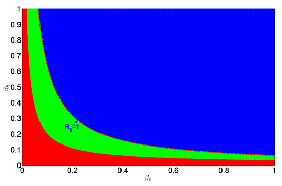
Figure 2. Regional distribution of equilibria in system (2) as functions of ${\beta }_v$ and ${\beta }_h$. The red, blue, and green regions correspond to the absence of endemic equilibria, the presence of a unique endemic equilibrium, and the coexistence of two endemic equilibria, respectively.

As the basic reproduction number $R_0$ serves as a critical epidemiological threshold, we construct a bifurcation diagram in the $(R_0,I_h)$ parameter plane to characterize system dynamics. To comprehensively illustrate bifurcation types, we select two distinct values for the parameter $\alpha$: $\alpha =0.005$ and $\alpha =0.0012$.

When $\alpha =0.005>{\alpha }^{\ast }$, system (2) undergoes backward bifurcation at $R_0=1$ (Figure 3). In the sub-threshold regime ($R_0<1$), three coexisting equilibria emerge: a stable disease-free equilibrium and two endemic equilibria (one stable, one unstable). This bistability is further characterized by an additional critical threshold $R_0^c=0.703$, identified through saddle-node bifurcation analysis. The hysteresis loop between $R_0^c$ and $R_0=1$ implies three key insights: (i) Temporary control measures that reduce $R_0$ below 1 but may fail to achieve permanent eradication above 0.703. (ii) Long-term HLB persistence can occur even with $R_0<1$ due to the basin stability of the endemic state. (iii) Eradication requires a sustained intervention to push $R_0<R_0^c$, thereby breaking the basin of attraction for the endemic equilibrium.

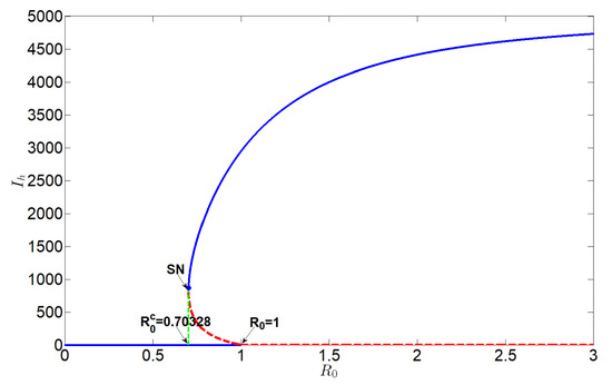
Figure 3. Backward bifurcation diagram of system (2), here the blue solid curve stands for stable, and the red dashed curve stands for unstable.

In contrast, Figure 4 demonstrates that system (2) exhibits a forward bifurcation at $R_0=1$, when $\alpha =0.0012<{\alpha }^{\ast }$. In this regime, no endemic equilibrium exists for $R_0<1$, confirming $R_0=1$ as an absolute eradication threshold for HLB. This indicates that maintaining $R_0<1$ through a continuous reduction of secondary infections guarantees disease elimination.

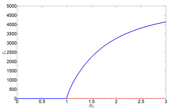
Figure 4. Forward bifurcation diagram of system (2), here the blue solid curve stands for stable, and the red dashed curve stands for unstable.

Next, we analyze how the basic reproduction number responds when the vector preference parameter and the removal rate of infected trees are altered simultaneously. As shown in Figure 5, $R_0$ increases with an ascending value of the preference parameter $\omega$ or a descending value of the removal rate $\delta$. The red line denotes the threshold where $R_0=1$, while the distinct colors (ranging from blue to yellow in two-step increments) illustrate $R_0$ values increasing from 0 to 11. These results highlight that both the preference behavior of psyllids and the control strategy of removing infected trees play key roles in HLB management.

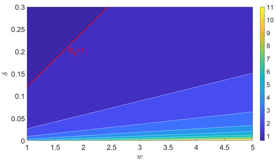
Figure 5. Contour plots of basic reproduction number $R_0$ with respect to $\omega$ and $\delta$, where ${\beta }_v=0.3$ and $\alpha =0.0005$.

Figure 6 displays the spatiotemporal sequence plots of system (9). With parameter settings $d_1=0,d_2=0.015$, and $\alpha =0.0012$, $R_0=0.6547<1$, showing the disease will be eradicated (see Figure 6a,b). Conversely, when $\alpha =0.005$, $R_0=5.8923>1$, indicating the disease will become endemic (see Figure 6c,d). These results validate the conclusions of Theorem 7.

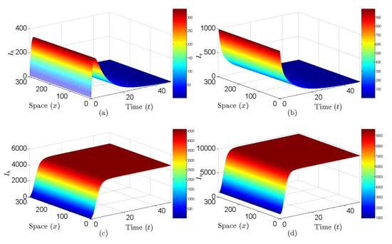
Figure 6. Figures show that movement paths of $I_h$ and $I_v$ as functions of $(t,x)$ of spatial system (9). (a,b) $R_0=0.6547<1$, the disease will die out. (c,d) $R_0=5.8923>1$, the disease is permanent.

6. Conclusions and Discussion

This study advances our understanding of HLB transmission dynamics by integrating two critical, yet previously underexplored, factors into a compartmental model: saturated removal rates of infected trees and vector behavioral bias. The incorporation of saturated removal rates reflects real-world limitations in detecting and eliminating infected trees. Unlike linear removal assumptions in prior models, saturation acknowledges that delayed interventions (e.g., due to diagnostic lag or resource constraints) allow infections to accumulate nonlinearly, amplifying outbreak risks. Simultaneously, vector behavioral bias, i.e., the preferential movement of psyllids toward infected trees, captures a key ecological feedback loop: infected hosts attract more vectors, accelerating pathogen spread. Together, these mechanisms explain why traditional models, which neglect these factors, may underestimate HLB’s persistence and resurgence potential.

Next, we will systematically review the main theoretical research achievements of this paper and deeply explore the guiding significance and practical implications of these theoretical insights for actual disease management.

The basic reproduction number $R_0$ is a cornerstone for predicting outbreak thresholds. However, our analysis reveals the following dynamic behavior. (i) Subcritical Bistability ($R_0<1$): When $R_0$ falls below 1, the system can exhibit bistability, where both disease-free and endemic equilibria coexist. This implies that even if $R_0$ is suppressed below the canonical threshold, pre-existing infections or transient vector surges could trigger outbreaks. (ii) Supercritical Uniqueness ($R_0>1$): When $R_0$ exceeds 1, the system converges to a unique endemic equilibrium, independent of initial conditions. This aligns with the classical epidemic theory. Therefore, eradication requires not only reducing $R_0$ but also managing initial infection loads to avoid bistable traps.

Delayed removal triggers backward bifurcation: Conversely, slow removal of infected trees ($\alpha >{\alpha }^{\ast }$) induces backward bifurcation, creating a subcritical threshold ($R_0^c<1$) where endemicity persists even with $R_0<1$. This mirrors challenges in managing diseases like tuberculosis, where delayed diagnosis undermines containment. Consequently, rapid removal of infected trees ($\alpha <{\alpha }^{\ast }$) is non-negotiable when the aim is to avoid backward bifurcation’s destabilizing effects.

Contrary to initial expectations, reaction–diffusion processes did not alter equilibrium stability in our analysis. This finding suggests that homogeneous mixing assumptions may adequately characterize HLB spread at regional scales, implying that simplified models without explicit spatial dynamics could still capture key transmission mechanisms. Notably, spatial heterogeneity appears to play a secondary role compared to temporal factors, like the delayed removal of infected trees, which have been shown to significantly influence bistability and outbreak thresholds.

While reaction–diffusion dynamics did not impact equilibrium stability in the current model, future research could explore how spatial heterogeneity, such as variability in orchard layouts or seasonal psyllid migration patterns, might modulate disease spread under different management scenarios. By integrating these dynamical principles into agricultural practices, stake holders can develop more targeted strategies to mitigate HLB’s devastating impact on citrus production.

References

- Bové, J.M. Huanglongbing: A destructive, newly-emerging, century-old disease of citrus. J. Plant Pathol. 2006, 88, 7–37. [Google Scholar]
- Hall, D.G.; Richardson, M.L.; Ammar, E.D.; Halbert, S.E. Asian citrus psyllid, Diaphorina citri, vector of citrus huanglongbing disease. Entomol. Exp. Appl. 2013, 146, 207–223. [Google Scholar] [CrossRef]
- Mann, R.S.; Qureshi, J.A.; Stansly, P.A.; Stelinski, L.L. Behavioral response of Tamarixia radiata (Waterston) (Hymenoptera: Eulophidae) to volatiles emanating from Diaphorina citri Kuwayama (Hemiptera: Psyllidae) and citrus. J. Insect Behav. 2010, 23, 447–458. [Google Scholar] [CrossRef]
- Zhang, F.M.; Qiu, Z.P.; Zhong, B.L.; Feng, T.; Huang, A.J. Modeling citrus Huanglongbing transmission within an orchard and its optimal control. Math. Biosci. Eng. 2020, 17, 2048–2069. [Google Scholar] [CrossRef] [PubMed]
- Luo, L.; Gao, S.J.; Ge, Y.Q.; Luo, Y.Q. Transmission dynamics of a Huanglongbing model with cross protection. Adv. Differ. Equ. 2017, 2017, 355. [Google Scholar] [CrossRef]
- Chiyaka, C.; Singer, B.H.; Halbert, S.E.; Morris, J.G., Jr.; van Bruggen, A.H. Modeling huanglongbing transmission within a citrus tree. Proc. Natl. Acad. Sci. USA 2012, 109, 12213–12218. [Google Scholar] [CrossRef] [PubMed]
- Zhang, X.; Liu, X.N. Backward bifurcation of an epidemic model with saturated treatment function. J. Math. Anal. Appl. 2008, 348, 433–443. [Google Scholar] [CrossRef]
- Yang, Y.; Zou, L.; Zhou, J.L.; Hsu, C.H. Dynamics of a waterborne pathogen model with spatial heterogeneity and general incidence rate. Nonlinear Anal. Real World Appl. 2020, 53, 103065. [Google Scholar] [CrossRef]
- Cai, Y.L.; Lian, X.Z.; Peng, Z.H.; Wang, W.M. Spatiotemporal transmission dynamics for influenza disease in a heterogenous environment. Nonlinear Anal. Real World Appl. 2019, 46, 178–194. [Google Scholar] [CrossRef]
- Goldbeter, A. Oscillatory enzyme reactions and Michaelis–Menten kinetics. FEBS Lett. 2013, 587, 2778–2784. [Google Scholar] [CrossRef] [PubMed]
- Van den Driessche, P.; Watmough, J. Reproduction numbers and sub-threshold endemic equilibria for compartmental models of disease transmission. Math. Biosci. 2002, 180, 29–48. [Google Scholar] [CrossRef] [PubMed]
- Castillo-Chavez, C.; Song, B.J. Dynamical models of tuberculosis and their applications. Math. Biosci. Eng. 2004, 1, 361–404. [Google Scholar] [CrossRef] [PubMed]
- Zhang, T.H.; Zhang, T.Q.; Meng, X.Z. Stability analysis of a chemostat model with maintenance energy. Appl. Math. Lett. 2017, 68, 1–7. [Google Scholar] [CrossRef]
- Tang, Z. Preliminary Study of Orchard Monitoring and Planning Model. Ph.D. Thesis, Huazhong Agricultural University, Wuhan, China, 2012. (In Chinese). [Google Scholar]
- Vilamiu, R.; Ternes, S.; Braga, G.; Laranjeira, F. A model for Huanglongbing spread between citrus plants including delay times and human intervention. AIP Conf. Proc. 2012, 1479, 2315–2319. [Google Scholar]
Disclaimer/Publisher’s Note: The statements, opinions and data contained in all publications are solely those of the individual author(s) and contributor(s) and not of MDPI and/or the editor(s). MDPI and/or the editor(s) disclaim responsibility for any injury to people or property resulting from any ideas, methods, instructions or products referred to in the content. |
© 2025 by the authors. Licensee MDPI, Basel, Switzerland. This article is an open access article distributed under the terms and conditions of the Creative Commons Attribution (CC BY) license (https://creativecommons.org/licenses/by/4.0/).