A Linearized Conservative Finite Difference Scheme for the Rosenau–RLW Equation

Abstract

A novel two–level linearized conservative finite difference method is proposed for solving the initial boundary value problem of the Rosenau–RLW equation. To preserve the energy conservation property, the Crank–Nicolson scheme is employed for temporal discretization, combined with an averaging treatment of the nonlinear term between the nth and $(n+1)$th time levels. For spatial discretization, a centered symmetric scheme is adopted. Meanwhile, the discrete conservation law is presented, and the existence and uniqueness of the numerical solutions are rigorously proved. Furthermore, the convergence and stability of the scheme are analyzed using the discrete energy method. Numerical experiments validate the theoretical results.

1. Introduction

The regularized long wave (RLW) equation

$$u_t+u_x+u{u}_x-u_{xxt}=0,$$

(1)

was originally proposed by Peregrine [1,2] to describe undular bore behavior. This equation overcomes the limitations of the traditional Korteweg–de Vries (KdV) equation in modeling long-wave propagation, making it more suitable for simulating physical phenomena such as shallow water waves and plasma waves. Its advantage lies in its improved capability to capture both dispersive and nonlinear wave effects while maintaining higher numerical stability [3,4]. However, subsequent studies revealed that the RLW Equation (1) cannot adequately describe wave–wave and wave–wall interactions. To address this limitation, Rosenau [5,6] proposed the following modified equation:

$$u_t+u_{xxxxt}+u_x+u{u}_x=0,$$

(2)

which can also be applied to model dense discrete systems and simulate long-chain transmission in L–C circuits for radio and computer applications. The solitary wave solutions of Equation (2) have been extensively investigated numerically [7,8].

To more accurately describe more complex wave motions, if a viscous term $-u_{xxt}$ is added into the Rosenau Equation (2), we can obtain the following new equation, which combines the Rosenau Equation (2) and the RLW Equation (1):

$$u_t-u_{xxt}+u_{xxxxt}+u_x+u{u}_x=0.$$

(3)

This equation, referred to as the Rosenau–RLW equation, incorporates the strong dispersive effects of the Rosenau Equation (2) and the nonlinear characteristics of the RLW Equation (1). It is primarily used to model nonlinear dispersive phenomena in fluid dynamics and wave propagation, including the propagation and interaction of nonlinear waves (for example, solitary waves) in shallow water environments, the propagation of optical pulses in dispersive media, and wave-breaking phenomena in nonlinear dynamics. Specifically, the high-order dispersive term $u_{xxxxt}$ can represent high-order dispersion, accounting for more refined wave dispersion effects beyond the standard second term. It also can help model short-wavelength behavior and stabilize solutions by counteracting nonlinear steepening. The dissipative term $u_{xxt}$ typically introduces weak dissipation or damping, balancing energy growth from nonlinearity. For nonlinear convection term $u{u}_x$, it is fundamental to wave steepening and shock formation (e.g., in Burgers’ equation).

However, due to its nonlinearity, the Rosenau–RLW Equation (3) generally does not admit analytical solutions. Therefore, developing numerical methods is crucial for gaining deeper insight into its solution behavior. In this paper, we consider the following initial and boundary value problem of the Rosenau–RLW equation,

$$\begin{array}{ccc}& & u_t-u_{xxt}+u_{xxxxt}+u_x+u{u}_x=0,(x,t)\in (x_L,x_R)\times (0,T],\hfill \end{array}$$

(4)

$$\begin{array}{ccc}& & u(x,0)=u_0\left(x\right),x\in [x_L,x_R],\hfill \end{array}$$

(5)

$$\begin{array}{ccc}& & u(x_L,t)=u(x_R,t)=0,u_{xx}(x_L,t)=u_{xx}(x_R,t)=0,t\in [0,T],\hfill \end{array}$$

(6)

where $u_0\left(x\right)$ is a known function. The initial boundary value problem (4)–(6) possesses the conservative quantity [9],

$$\begin{array}{c}\hfill Q\left(t\right)={\int }_{x_L}^{x_R}u(x,t)dx={\int }_{x_L}^{x_R}{u}_0(x,t)dx=Q\left(0\right),\end{array}$$

(7)

where $Q\left(0\right)$ is a constant determined solely by the initial condition. Since the physical boundary condition of Rosenau–RLW Equation (3) satisfies

$$\begin{array}{c}\hfill u(x,t)\to 0,u_{xx}(x,t)\to 0,(t>0),\mathrm{as}\left|x\right|\to \infty .\end{array}$$

when $-x_L\gg 0$ and $x_R\gg 0$, the boundary condition (6) is reasonable for the numerical investigation.

Numerous numerical methods have been developed to study the standard Rosenau–RLW equation and its generalized form. Among these, the finite difference method [9,10,11,12,13,14,15,16,17,18] has attracted considerable attention from scholars due to its convenience in constructing numerical grids. For instance, Pan et al. [10] proposed a Crank–Nicolson-type finite difference scheme and proved its unconditional stability, second-order convergence, and uniqueness. Similarly, Zuo et al. [11] developed an analogous scheme for the generalized case. It is worth noting that, owing to the nonlinearity of these schemes, the existence of their different solutions must be established using the Brouwer fixed-point theorem. In addition to nonlinear schemes, several linearized approaches have been explored. For example, Pan et al. [13] introduced an average three-level linearized conservative difference method. Meanwhile, Hu et al. [9] proposed an improved version with higher spatial accuracy. Wang et al. [12] developed a three-level finite difference scheme incorporating two weighted parameters applied to first-order derivatives in both time and space variables. To further enhance spatial accuracy, Wongsaijai et al. [15,16] constructed a nonlinear compact scheme and a pseudo-compact scheme, respectively. Beyond the finite difference method, other effective numerical techniques have been applied to the Rosenau–RLW equation, including the finite element method [19,20,21], the Strang time-splitting method [22], the B-spline allocation method [23], the multiple integral finite volume method [24]. For high-dimensional cases of the Rosenau–RLW equation, readers may refer to [25,26,27,28].

In fact, the aforementioned numerical schemes can be classified into two categories: two-level nonlinear schemes and three-level linear schemes. The advantage of a nonlinear two-level scheme lies in its generally higher numerical accuracy; however, each computation requires multiple iterations, and thus, significant computational time. Although the three-level scheme is linear, its drawback is that it cannot self-start and requires the use of another scheme to calculate the numerical solution at the second level to supplement the initial data.

In this paper, we propose a two-level linearized conservative difference scheme for the initial and boundary value problem of the Rosenau–RLW Equation (4)–(6). In the temporal direction, based on the traditional Crank–Nicolson method, the nonlinear term is averaged between the nth and $(n+1)$th levels to ensure that the scheme maintains second-order accuracy. For the spatial discretization, a central symmetric technique is adopted to construct a difference scheme with a theoretical accuracy of $O({\tau }^2+h^2)$, which can effectively simulate the conservative quantity (7). Regarding the theoretical analysis, due to the absence of a prior error estimate for the numerical solution of this scheme, we employ the Sobolev embedding inequality to rigorously prove the convergence and stability of the proposed scheme.

The remainder of this paper is organized as follows. Section 2 introduces the necessary notations and preliminary lemmas. In Section 3, we present the finite difference scheme and discuss its conservation laws. In Section 4, the existence and uniqueness of numerical solutions are established. The convergence and stability of the proposed scheme are rigorously analyzed in Section 5. Finally, in Section 6, numerical experiments are described; these validate the theoretical findings and demonstrate the efficiency of the proposed scheme.

2. Notations and Preliminaries

Consider the domain $\mathsf{\Omega }=[x_L,x_R]\times [0,T]$. Denote $h=(x_R-x_L)/J$ as the step size for the spatial grid and $\tau$ as the step size for the temporal direction, such that $x_j=x_L+jh(0\le j\le J)$, $t_n=n\tau$ $(n=0,1,2,\cdots ,N,N=[T/\tau \left]\right)$. Let $u_j^n=u(x_j,t_n)$ be the exact value of $u(x,t)$ and $U_j^n\approx u(x_j,t_n)$ be the approximation of $u(x,t)$ at the point $(x_j,t_n)$, respectively. Then, $e_j^n=u_j^n-U_j^n$ is the error between $u_j^n$ and $U_j^n$. In what follows, C denotes a general positive constant, which may have different values in different occurrences. Define

$$\begin{array}{ccc}& & {\left(U_j^n\right)}_t={\displaystyle \frac{U_j^{n+1}-U_j^n}{\tau }},{\left(U_j^n\right)}_x={\displaystyle \frac{U_{j+1}^n-U_j^n}{h}},{\left(U_j^n\right)}_{\overline{x}}={\displaystyle \frac{U_j^n-U_{j-1}^n}{h}},\hfill \\ & & {\left(U_j^n\right)}_{\widehat{x}}={\displaystyle \frac{U_{j+1}^n-U_{j-1}^n}{2h}},U_j^{n+\frac{1}{2}}={\displaystyle \frac{U_j^{n+1}+U_j^n}{2}},\hfill \\ & & \langle U^n,V^n\rangle =h\sum _{j=1}^{J-1}{U}_j^n{V}_j^n,{\parallel U^n\parallel }^2=\langle U^n,U^n\rangle ,{\parallel U^n\parallel }_{\infty }=\underset{1\le j\le J-1}{max}\left|U_j^n\right|,\hfill \\ & & Z_h^0=\{U=\left(U_j\right)|U_{-1}=U_0=U_J=U_{J+1}=0,j=-1,0,\cdots ,J,J+1\}.\hfill \end{array}$$

Firstly, we present some lemmas that will be used in the subsequent analysis.

Lemma 1 

(Summation by Parts [29]). For any mesh functions $U=\left\{U_j\right|j=0,1,2,\cdots ,J\}$ and $V=\left\{V_j\right|j=0,1,2,\cdots ,J\}$, we have

$$\begin{array}{c}\hfill h\sum _{j=0}^{J-1}{\left(V_j\right)}_x{U}_j=-h\sum _{j=1}^J{V}_j{\left(U_j\right)}_{\overline{x}}+V_J{U}_J-V_0{U}_0\end{array}$$

and

$$\begin{array}{c}\hfill h\sum _{j=1}^{J-1}\left(U_j\right){\left(V_j\right)}_{x\overline{x}}=-h\sum _{j=0}^{J-1}{\left(U_j\right)}_x{\left(U_j\right)}_x+U_J{\left(V_J\right)}_{\overline{x}}-U_0{\left(V_0\right)}_x.\end{array}$$

Lemma 2 

([30]). For $\forall U\in Z_h^0$, the following result

$$\begin{array}{c}\hfill {\parallel U_{\widehat{x}}\parallel }^2\le {\parallel U_x\parallel }^2\end{array}$$

holds.

Lemma 3 

(The discrete Sobolev inequality [29]). Let $U=\left\{U_j\right|j=0,1,2,\cdots ,J\}$ be a mesh function defined on the interval $[x_L,x_R]$. Then, the following inequality holds:

$$\begin{array}{c}\hfill {\parallel U\parallel }_{\infty }\le C_0\sqrt{\parallel U\parallel }\sqrt{\parallel U_x\parallel +\parallel U\parallel },\end{array}$$

where $C_0$ is a constant which is independent of both U and h.

Lemma 4 

([29]). Let $U=\left\{U_j\right|j=0,1,2,\cdots ,J\}$ be a mesh function defined on $[x_L,x_R]$. Then, the following inequality holds:

$$\begin{array}{c}\hfill {\parallel U\parallel }_{\infty }\le C_1\parallel U_x\parallel +C_2\parallel U\parallel ,\end{array}$$

where $C_1$ and is $C_2$ are constants which are independent of both U and h.

Lemma 5 

(The discrete Gronwall inequality [29]). Let $\left\{w^n\right|n=0,1,2,\cdots ,N;$ $N\tau \le T\}$ be a non-negative mesh function satisfying the inequality $w^n\le A+\tau {\sum }_{l=1}^n{B}_l{w}^l$, where A and $B_l$ ($l=0,1,2,\cdots ,N$) are non-negative constants. Then,

$$\begin{array}{c}\hfill \underset{1\le n\le N}{max}\left|w^n\right|\le Aexp(2\tau \sum _{l=1}^N{B}_l)\end{array}$$

for $0\le n\le N$, provided that τ is sufficiently small that $\tau ·({max}_{1\le n\le N}{B}_l)\le \frac{1}{2}$.

Lemma 6 

([17]). Let $u_0\in H^2$. Then, the solution to problem (4)–(6) satisfies the following estimates:

$$\begin{array}{c}\hfill {\parallel u\parallel }_{L_2}\le C,{\parallel u_x\parallel }_{L_2}\le C,{\parallel u_{xx}\parallel }_{L_2}\le C,{\parallel u\parallel }_{L_{\infty }}\le C.\end{array}$$

where C is a constant independent of u.

3. Finite Difference Scheme and Discrete Conservation Laws

Supposing that $u(x,t)$ is smooth enough, by the Taylor expansion, the following results hold

$$\begin{array}{ccc}& & {(u_j^n)}_{\widehat{x}}={({\displaystyle \frac{\partial u}{\partial x}})}_j^n+O(h^2),\hfill \end{array}$$

(8)

$$\begin{array}{ccc}& & u_j^n=u_j^{n+\frac{1}{2}}-{\displaystyle \frac{\tau }{2}}{({\displaystyle \frac{\partial u}{\partial t}})}_j^{n+\frac{1}{2}}+O({\tau }^2),\hfill \end{array}$$

(9)

$$\begin{array}{ccc}& & u_j^{n+1}=u_j^{n+\frac{1}{2}}+{\displaystyle \frac{\tau }{2}}{({\displaystyle \frac{\partial u}{\partial t}})}_j^{n+\frac{1}{2}}+O({\tau }^2)\hfill \end{array}$$

(10)

when $h,\tau \to 0$. Let

$$\begin{array}{c}\hfill A=\frac{1}{2}{({\displaystyle \frac{\partial u}{\partial t}})}_j^{n+\frac{1}{2}},B={\displaystyle \frac{1}{2}}{({\displaystyle \frac{{\partial }^{2}u}{\partial x\partial t}})}_j^{n+\frac{1}{2}}.\end{array}$$

Then, it follows from (8)–(10) that

$$\begin{array}{ccc}& & {\displaystyle \frac{1}{2}}{u}_j^n{(u_j^{n+1})}_{\widehat{x}}+{\displaystyle \frac{1}{2}}{u}_j^{n+1}{(u_j^n)}_{\widehat{x}}\hfill \\ & & ={\displaystyle \frac{1}{2}}(u_j^{n+\frac{1}{2}}-A\tau )·[{({\displaystyle \frac{\partial u}{\partial x}})}_j^{n+\frac{1}{2}}+B\tau ]+{\displaystyle \frac{1}{2}}(u_j^{n+\frac{1}{2}}+A\tau )·[{({\displaystyle \frac{\partial u}{\partial x}})}_j^{n+\frac{1}{2}}-B\tau ]+O({\tau }^2+h^2)\hfill \\ & & =u_j^{n+\frac{1}{2}}·{({\displaystyle \frac{\partial u}{\partial x}})}_j^{n+\frac{1}{2}}-AB{\tau }^2+O({\tau }^2+h^2)\hfill \\ & & ={(u{\displaystyle \frac{\partial u}{\partial x}})}_j^{n+\frac{1}{2}}+O({\tau }^2+h^2).\hfill \end{array}$$

(11)

For the problem (4)–(6), the following two-level linear finite difference scheme is constructed:

$$\begin{array}{ccc}& & {(U_j^n)}_t-{(U_j^n)}_{x\overline{x}t}+{(U_j^n)}_{xx\overline{x}\overline{x}t}+{(U_j^{n+\frac{1}{2}})}_{\widehat{x}}+\varphi (U_j^n,U_j^{n+1})=0,\hfill \\ & & j=1,2,\cdots ,J-1;n=2,3,\cdots ,N-1,\hfill \end{array}$$

(12)

$$\begin{array}{ccc}& & U_j^0=u_0(x_j),j=0,1,2,\cdots ,J,\hfill \end{array}$$

(13)

$$\begin{array}{ccc}& & U^n\in Z_h^0,n=0,1,2,\cdots ,N\hfill \end{array}$$

(14)

where

$$\begin{array}{c}\hfill \varphi (U_j^n,U_j^{n+1})={\displaystyle \frac{1}{2}}\left[U_j^n{(U_j^{n+1})}_{\widehat{x}}+U_j^{n+1}{(U_j^n)}_{\widehat{x}}\right].\end{array}$$

The following theorem shows how the difference scheme (12)–(14) simulates the conservative law numerically.

Theorem 1. 

Define the discrete energy:

$$\begin{array}{c}\hfill Q^n=h\sum _{j=1}^{J-1}{U}_j^n.\end{array}$$

Then, the difference scheme (12)–(14) is conservative for $Q^n$, i.e.,

$$\begin{array}{c}\hfill Q^n=Q^{n-1}=\cdots =Q^0\end{array}$$

(15)

for $n=1,2,\cdots ,N$.

Proof of Theorem 1. 

Noting that

$$\begin{array}{c}\hfill h\sum _{j=1}^{J-1}{(U_j^n)}_{x\overline{x}t}=0,h\sum _{j=1}^{J-1}{(U_j^n)}_{xx\overline{x}\overline{x}t}=0,h\sum _{j=1}^{J-1}{(U_j^{n+\frac{1}{2}})}_{\widehat{x}}=0,\end{array}$$

(16)

from Lemma 1 and the boundary condition (14), we have

$$\begin{array}{ccc}\hfill h\sum _{j=1}^{J-1}\varphi (U_j^n,U_j^{n+1})& =& {\displaystyle \frac{1}{2}}h\sum _{j=1}^{J-1}{U}_j^n{(U_j^{n+1})}_{\widehat{x}}+{\displaystyle \frac{1}{2}}h\sum _{j=1}^{J-1}{U}_j^{n+1}{(U_j^n)}_{\widehat{x}}\hfill \\ & =& {\displaystyle \frac{1}{2}}h\sum _{j=1}^{J-1}{U}_j^n{(U_j^{n+1})}_{\widehat{x}}-{\displaystyle \frac{1}{2}}h\sum _{j=1}^{J-1}{(U_j^{n+1})}_{\widehat{x}}{U}_j^n\hfill \\ & =& 0.\hfill \end{array}$$

Multiplying both sides of (12) by h, and summing it for j from 1 to $J-1$, we obtain

$$\begin{array}{c}\hfill h\sum _{j=1}^{J-1}{(U_j^n)}_t=0.\end{array}$$

(17)

Finally, multiplying both sides of (17) by $\tau$, by the definition of $Q^n$, we can get (15). □

Remark 1. 

In fact, in addition to mass conservation, the Rosenau–RLW Equation (3) also possesses the property of energy conservation [9]. However, due to the extrapolated linearization treatment of the nonlinear term in this numerical scheme, its discrete energy is no longer conserved.

4. Existence and Uniqueness of Numerical Solutions

Next, we use mathematical induction to analyze the existence and uniqueness of numerical solutions for difference schemes (12)–(14).

Theorem 2. 

If the time step τ is small enough, the numerical solutions of difference scheme (12)–(14) are unique.

Proof of Theorem 2. 

Obviously, it follows from (13) that $U^0$ is uniquely determined by the initial condition. Suppose that $U^n(n\le N-1)$ is the unique solution to scheme (12)–(14) and

$$\begin{array}{c}\hfill {\parallel U^n\parallel }_{\infty }\le C,n\le N-1.\end{array}$$

(18)

Now, we prove that there is a unique $U^{n+1}$ which also satisfies (12)–(14).

Consider the homogeneous linear equation system corresponding to Equation (12),

$$\begin{array}{ccc}& & {\displaystyle \frac{1}{\tau }}{U}_j^{n+1}-{\displaystyle \frac{1}{\tau }}{(U_j^{n+1})}_{x\overline{x}}+{\displaystyle \frac{1}{\tau }}{(U_j^{n+1})}_{xx\overline{x}\overline{x}}+{\displaystyle \frac{1}{2}}{(U_j^{n+1})}_{\widehat{x}}+\varphi (U_j^n,U_j^{n+1})=0,\hfill \\ & & j=1,2,\cdots ,J-1;n=0,1,2,\cdots ,N-1.\hfill \end{array}$$

(19)

Taking the inner product of (19) with $U^{n+1}$, by Lemma 1, the boundary condition (14), and the following result:

$$\begin{array}{c}\hfill \langle U_{\widehat{x}}^{n+1},U^{n+1}\rangle =0,\end{array}$$

one can get

$$\begin{array}{c}\hfill {\displaystyle \frac{1}{\tau }}\parallel U^{n+1}{\parallel }^2+{\displaystyle \frac{1}{\tau }}\parallel U_x^{n+1}{\parallel }^2+{\displaystyle \frac{1}{\tau }}\parallel U_{x\overline{x}}^{n+1}{\parallel }^2=-\langle \varphi (U^n,U^{n+1}),U^{n+1}\rangle .\end{array}$$

(20)

Combining Lemma 2 and the Cauchy–Schwarz inequality with (18), we have

$$\begin{array}{ccc}\hfill -\langle \varphi (U^n,U^{n+1}),U^{n+1}\rangle & =& -{\displaystyle \frac{1}{2}}h\sum _{j=1}^{J-1}\left[U_j^n{(U_j^{n+1})}_{\widehat{x}}+U_j^{n+1}{(U_j^n)}_{\widehat{x}}\right]U_j^{n+1}\hfill \\ & =& -{\displaystyle \frac{1}{2}}h\sum _{j=1}^{J-1}{U}_j^n{(U_j^{n+1})}_{\widehat{x}}{U}_j^{n+1}-{\displaystyle \frac{1}{2}}h\sum _{j=1}^{J-1}{U}_j^{n+1}{(U_j^n)}_{\widehat{x}}{U}_j^{n+1}\hfill \\ & =& -{\displaystyle \frac{1}{2}}h\sum _{j=1}^{J-1}{U}_j^n{(U_j^{n+1})}_{\widehat{x}}{U}_j^{n+1}+{\displaystyle \frac{1}{2}}h\sum _{j=1}^{J-1}{\left[{(U_j^{n+1})}^2\right]}_{\widehat{x}}{U}_j^n\hfill \\ & =& -{\displaystyle \frac{1}{2}}h\sum _{j=1}^{J-1}{U}_j^n{(U_j^{n+1})}_{\widehat{x}}{U}_j^{n+1}+{\displaystyle \frac{1}{2}}h\sum _{j=1}^{J-1}{U}_j^n(U_{j+1}^{n+1}+U_{j-1}^{n+1}){(U_j^{n+1})}_{\widehat{x}}\hfill \\ & \le & Ch\sum _{j=1}^{J-1}|{(U_j^{n+1})}_{\widehat{x}}|·|U_j^{n+1}|+Ch\sum _{j=1}^{J-1}|U_{j+1}^{n+1}|+|U_{j-1}^{n+1}|·|{(U_j^{n+1})}_{\widehat{x}}|\hfill \\ & \le & C({\parallel U_{\widehat{x}}^{n+1}\parallel }^2+{\parallel U^{n+1}\parallel }^2)\hfill \\ & \le & C({\parallel U_x^{n+1}\parallel }^2+{\parallel U^{n+1}\parallel }^2).\hfill \end{array}$$

(21)

Therefore, it follows from (20) and (21) that

$$\begin{array}{c}\hfill {\parallel U^{n+1}\parallel }^2+{\parallel U_x^{n+1}\parallel }^2+{\parallel U_{x\overline{x}}^{n+1}\parallel }^2\le C\tau ({\parallel U_x^{n+1}\parallel }^2+{\parallel U^{n+1}\parallel }^2)\end{array}$$

that is,

$$\begin{array}{c}\hfill (1-C\tau ){\parallel U^{n+1}\parallel }^2+(1-C\tau ){\parallel U_x^{n+1}\parallel }^2+{\parallel U_{x\overline{x}}^{n+1}\parallel }^2\le 0.\end{array}$$

If $1-C\tau >0$, the homogeneous linear equation system (19) about $\left\{U_j^{n+1}\right\}$ has only a zero solution. This completes the proof. □

5. Convergence and Stability of Numerical Solutions

By applying the Taylor expansion, we can derive the following truncation error of the scheme (12)–(14),

$$\begin{array}{ccc}& & r_j^n={(u_j^n)}_t-{(u_j^n)}_{x\overline{x}t}+{(u_j^n)}_{xx\overline{x}\overline{x}t}+{(u_j^{n+\frac{1}{2}})}_{\widehat{x}}+\varphi (u_j^n,u_j^{n+1})\hfill \end{array}$$

(22)

$$\begin{array}{ccc}& & u_j^0=u_0(x_j),j=0,1,2,\cdots ,J-1,J,\hfill \end{array}$$

(23)

$$\begin{array}{ccc}& & u^n\in Z_h^0,n=0,1,2,\cdots ,N-1,N.\hfill \end{array}$$

(24)

Clearly, if $\tau ,h\to 0$, the following result holds:

$$\begin{array}{c}\hfill |r_j^n|=O({\tau }^2+h^2).\end{array}$$

(25)

Theorem 3. 

Let $u_0\in H^2$. Then, the solution $U^n$ of scheme (12)–(14) converges to the continuous solution $u(x,t)$ of problem (4)–(6) of the order $O({\tau }^2+h^2)$ by the norm ${\parallel ·\parallel }_{\infty }$, provided that both τ and h are sufficiently small.

Proof of Theorem 3. 

Denote: $e_j^n=u_j^n-U_j^n$. Subtracting (22)–(24) from (12)–(14), we have

$$\begin{array}{ccc}& & r_j^n={(e_j^n)}_t-{(e_j^n)}_{x\overline{x}t}+{(e_j^n)}_{xx\overline{x}\overline{x}t}+{(e_j^{n+\frac{1}{2}})}_{\widehat{x}}+\varphi (u_j^n,u_j^{n+1})-\varphi (U_j^n,U_j^{n+1}),\hfill \\ & & j=1,2,\cdots ,J-1,n=1,2,\cdots ,N-1,\hfill \end{array}$$

(26)

$$\begin{array}{ccc}& & e_j^0=0,j=0,1,2,\cdots ,J-1,J,\hfill \end{array}$$

(27)

$$\begin{array}{ccc}& & e^n\in Z_h^0,n=0,1,2,\cdots ,N-1,N.\hfill \end{array}$$

(28)

By Lemma 6 and (25), there exist constants $C_u$ and $C_r$, independent of $\tau$ and h such that

$$\begin{array}{c}\hfill {\parallel u^n\parallel }_{\infty }\le C_u,{\parallel r^n\parallel }_{\infty }\le C_r({\tau }^2+h^2),n=1,2,\cdots ,N-1.\end{array}$$

(29)

From (13) and (27), we have

$$\begin{array}{c}\hfill \parallel e^0\parallel =0,{\parallel U^0\parallel }_{\infty }\le C_u.\end{array}$$

(30)

Assume that

$$\begin{array}{c}\hfill \parallel e^l\parallel +\parallel e_x^l\parallel +\parallel e_{xx}^l\parallel \le C_l({\tau }^2+h^2),l=1,2,\cdots ,n,(n\le N-1),\end{array}$$

(31)

where $C_l$ is a constant which is also independent of $\tau$ and h. Then, applying Lemma 3 and the Cauchy–-Schwarz inequality, we obtain

$$\begin{array}{ccc}\hfill {\parallel e^l\parallel }_{\infty }& \le & C_0\sqrt{\parallel e^l\parallel }\sqrt{\parallel e_x^l\parallel +\parallel e^l\parallel }\hfill \\ & \le & {\displaystyle \frac{1}{2}}{C}_0(2\parallel e^l\parallel +\parallel e_x^l\parallel )\hfill \\ & \le & {\displaystyle \frac{3}{2}}{C}_0{C}_l({\tau }^2+h^2),\hfill \end{array}$$

(32)

and

$$\begin{array}{c}\hfill {\parallel U^l\parallel }_{\infty }\le {\parallel u^l\parallel }_{\infty }+{\parallel e^l\parallel }_{\infty }\le C_u+{\displaystyle \frac{3}{2}}{C}_0{C}_l({\tau }^2+h^2),l=1,2,\cdots ,n.\end{array}$$

(33)

Taking the inner product of (26) with $2e^{n+\frac{1}{2}}$, from the boundary condition (28), Lemma 1, and the following result:

$$\begin{array}{c}\hfill \langle e_{\widehat{x}}^{n+\frac{1}{2}},e^{n+\frac{1}{2}}\rangle =0,\end{array}$$

we have

$$\begin{array}{c}\hfill \langle r^n,2e^{n+\frac{1}{2}}\rangle ={\parallel e^n\parallel }_t^2+{\parallel e_x^n\parallel }_t^2+{\parallel e_{xx}^n\parallel }_t^2+2\langle \varphi (u^n,u^{n+1})-\varphi (U^n,U^{n+1}),e^{n+\frac{1}{2}}\rangle ,\end{array}$$

(34)

Using the Mean Value Theorem yields

$$\begin{array}{c}\hfill {(u_j^{n+\frac{1}{2}})}_{\widehat{x}}={\displaystyle \frac{u(x_{j+1},\frac{t_n+t_{n+1}}{2})-u(x_{j-1},\frac{t_n+t_{n+1}}{2})}{2h}}={\displaystyle \frac{\partial }{\partial x}}u({\xi }_j,{\displaystyle \frac{t_n+t_{n+1}}{2}}),(x_{j-1}\le {\xi }_j\le x_{j+1}).\end{array}$$

Then, according to Lemma 6, we have

$$\begin{array}{c}\hfill {\parallel u_{\widehat{x}}^{n+\frac{1}{2}}\parallel }_{\infty }\le C.\end{array}$$

(35)

When the parameters $\tau$ and h are sufficiently small such that

$$\begin{array}{c}\hfill {\displaystyle \frac{3}{2}}{C}_0·(\underset{0\le l\le n}{max}{C}_l)({\tau }^2+h^2)\le 1,\end{array}$$

(36)

based on (33), (35), (36), Lemma 2, and the Cauchy–-Schwarz inequality, we have

$$\begin{array}{ccc}& & \langle \varphi (u^n,u^{n+1})-\varphi (U^n,U^{n+1}),2e^{n+\frac{1}{2}}\rangle \hfill \\ & & =h\sum _{j=1}^{J-1}[e_j^n{(u_j^{n+1})}_{\widehat{x}}+U_j^n{(e_j^{n+1})}_{\widehat{x}}]e_j^{n+\frac{1}{2}}+h\sum _{j=1}^{J-1}[u_j^{n+1}{(e_j^n)}_{\widehat{x}}+e_j^{n+1}{(U_j^n)}_{\widehat{x}}]e_j^{n+\frac{1}{2}}\hfill \\ & & =h\sum _{j=1}^{J-1}[e_j^n{(u_j^{n+1})}_{\widehat{x}}+U_j^n{(e_j^{n+1})}_{\widehat{x}}]e_j^{n+\frac{1}{2}}+h\sum _{j=1}^{J-1}{u}_j^{n+1}{(e_j^n)}_{\widehat{x}}{e}_j^{n+\frac{1}{2}}\hfill \\ & & -h\sum _{j=1}^{J-1}[U_j^n{(e_j^{n+1})}_{\widehat{x}}{e}_{j+1}^{n+\frac{1}{2}}+e_{j-1}^{n+1}{(e_j^{n+\frac{1}{2}})}_{\widehat{x}}]\hfill \\ & & \le {\displaystyle \frac{1}{2}}{C}_u({\parallel e^n\parallel }^2+{\parallel e_x^n\parallel }^2+2{\parallel e^{n+\frac{1}{2}}\parallel }^2)\hfill \\ & & +{\displaystyle \frac{1}{2}}[C_u+C_0{C}_1({\tau }^2+h^2)]({\parallel e^{n+1}\parallel }^2+2{\parallel e_x^{n+1}\parallel }^2+2{\parallel e^{n+\frac{1}{2}}\parallel }^2+{\parallel e_x^{n+\frac{1}{2}}\parallel }^2)\hfill \\ & & \le {\displaystyle \frac{1}{2}}{C}_u(2{\parallel e^n\parallel }^2+{\parallel e_x^n\parallel }^2+{\parallel e^{n+1}\parallel }^2)\hfill \\ & & +{\displaystyle \frac{1}{4}}(C_u+1)(4{\parallel e^{n+1}\parallel }^2+5{\parallel e_x^{n+1}\parallel }^2+2{\parallel e^n\parallel }^2+{\parallel e_x^n\parallel }^2),\hfill \end{array}$$

(37)

and

$$\begin{array}{c}\hfill \langle r^n,2e^{n+\frac{1}{2}}\rangle \le {\parallel r^n\parallel }^2+{\displaystyle \frac{1}{2}}({\parallel e^{n+1}\parallel }^2+{\parallel e^n\parallel }^2)\le {\parallel r^n\parallel }^2+{\parallel e^{n+1}\parallel }^2+{\parallel e^n\parallel }^2.\end{array}$$

(38)

where we employ the identity

$$\begin{array}{ccc}& & h\sum _{j=1}^{J-1}{e}_j^{n+1}{(U_j^n)}_{\widehat{x}}{e}_j^{n+\frac{1}{2}}=h\sum _{j=1}^{J-1}{e}_j^{n+1}{e}_j^{n+\frac{1}{2}}{(U_j^n)}_{\widehat{x}}=-h\sum _{j=1}^{J-1}{U}_j^n{(e_j^{n+1}{e}_j^{n+\frac{1}{2}})}_{\widehat{x}}\hfill \\ & & =-h\sum _{j=1}^{J-1}{U}_j^n{\displaystyle \frac{e_{j+1}^{n+1}{e}_{j+1}^{n+\frac{1}{2}}-e_{j-1}^{n+1}{e}_{j-1}^{n+\frac{1}{2}}}{2h}}\hfill \\ & & =-h\sum _{j=1}^{J-1}{U}_j^n{\displaystyle \frac{(e_{j+1}^{n+1}{e}_{j+1}^{n+\frac{1}{2}}-e_{j-1}^{n+1}{e}_{j+1}^{n+\frac{1}{2}})+(e_{j-1}^{n+1}{e}_{j+1}^{n+\frac{1}{2}}-e_{j-1}^{n+1}{e}_{j-1}^{n+\frac{1}{2}})}{2h}}\hfill \\ & & =-h\sum _{j=1}^{J-1}{U}_j^n[{(e_j^{n+1})}_{\widehat{x}}{e}_{j+1}^{n+\frac{1}{2}}+(e_{j-1}^{n+1}){(e_{j+1}^{n+\frac{1}{2}})}_{\widehat{x}}].\hfill \end{array}$$

Substituting (37) and (38) into (34) yields

$$\begin{array}{ccc}& & {\parallel e^n\parallel }_t^2+{\parallel e_x^n\parallel }_t^2+{\parallel e_{xx}^n\parallel }_t^2\hfill \\ & & \le \parallel r^n\parallel +{\parallel e^n\parallel }^2+{\parallel e^{n+1}\parallel }^2+{\displaystyle \frac{1}{4}}(C_u+1)(6{\parallel e^n\parallel }^2+3{\parallel e_x^n\parallel }^2+6{\parallel e^{n+1}\parallel }^2+5{\parallel e_x^{n+1}\parallel }^2)\hfill \\ & & \le \parallel r^n\parallel +{\parallel e^n\parallel }^2+{\parallel e^{n+1}\parallel }^2+2(C_u+1)({\parallel e^n\parallel }^2+{\parallel e_x^n\parallel }^2+{\parallel e^{n+1}\parallel }^2+{\parallel e_x^{n+1}\parallel }^2)\hfill \\ & & \le \parallel r^n\parallel +3(C_u+1)({\parallel e^n\parallel }^2+{\parallel e_x^n\parallel }^2+{\parallel e^{n+1}\parallel }^2+{\parallel e_x^{n+1}\parallel }^2).\hfill \end{array}$$

(39)

By multiplying (39) by $\tau$ and summing from 1 to n, we obtain

$$\begin{array}{ccc}& & {\parallel e^{n+1}\parallel }^2+{\parallel e_x^{n+1}\parallel }^2+{\parallel e_{xx}^{n+1}\parallel }^2\le {\parallel e^1\parallel }^2+{\parallel e_x^1\parallel }^2+{\parallel e_{xx}^1\parallel }^2+\tau \sum _{k=1}^n{\parallel r^k\parallel }^2\hfill \\ & & +9(C_u+1)\tau \sum _{k=1}^{n+1}({\parallel e^k\parallel }^2+{\parallel e_x^k\parallel }^2+{\parallel e_{xx}^k\parallel }^2).\hfill \end{array}$$

(40)

Also, we can see that

$$\begin{array}{c}\hfill \tau \sum _{k=1}^n{\parallel r^k\parallel }^2\le n\tau \underset{1\le k\le n}{max}{\parallel r^k\parallel }^2\le T{(C_r)}^2{({\tau }^2+h^2)}^2.\end{array}$$

(41)

Let $\tau$ be chosen to be sufficiently small such that

$$\begin{array}{c}\hfill \tau <{\displaystyle \frac{1}{18(C_u+1)}}\end{array}$$

(42)

From Lemma 5, the combination of (33), (34) and (42) leads to

$$\begin{array}{ccc}\hfill {\parallel e^{n+1}\parallel }^2+{\parallel e_x^{n+1}\parallel }^2+{\parallel e_{xx}^{n+1}\parallel }^2& \le & [T{(C_r)}^2+{(C_1)}^2]{({\tau }^2+h^2)}^2{e}^{2T\left[9(1+C_u)\right]}\hfill \\ & \le & {(C_{n+1})}^2{({\tau }^2+h^2)}^2,n=1,2,\cdots ,N-1\hfill \end{array}$$

where

$$\begin{array}{c}\hfill C_{n+1}=(\sqrt{T}{C}_r+C_1)exp(9T(C_u+1)).\end{array}$$

Clearly, $C_{n+1}$ is a constant, independent of n. Thus, by the induction,

$$\begin{array}{c}\hfill \parallel e^n\parallel \le O({\tau }^2+h^2),\parallel e_x^n\parallel \le O({\tau }^2+h^2),\parallel e_{xx}^n\parallel \le O({\tau }^2+h^2)\end{array}$$

hold for $n=1,2,\cdots ,N$. Finally, according to Lemma 4, we have

$$\begin{array}{c}\hfill {\parallel e^n\parallel }_{\infty }\le O({\tau }^2+h^2),n=1,2,\cdots ,N.\end{array}$$

This completes the proof. □

Theorem 4. 

Let $u_0\in H^2$. Then, under the condition that both τ and h are sufficiently small, the solution of scheme (12)–(14) satisfies

$$\begin{array}{c}\hfill {\parallel U^n\parallel }_{\infty }\le {\tilde{C}}_0,n=1,2,\cdots ,N,\end{array}$$

where ${\tilde{C}}_0$ is a constant independent of both τ and h.

Proof of Theorem 4. 

From Theorem 3, it follows that for sufficiently small $\tau$ and h that

$$\begin{array}{c}\hfill {\parallel U^n\parallel }_{\infty }\le {\parallel u^n\parallel }_{\infty }+{\parallel e^n\parallel }_{\infty }\le {\tilde{C}}_0.\end{array}$$

This completes the proof. □

Remark 2. 

According to Theorem 4, if τ and h are sufficiently small, the solution $U^n$ of scheme (12)–(14) is stable in the norm ${\parallel ·\parallel }_{\infty }$.

6. Algorithm and Numerical Experiments

6.1. Algorithm

For the convenience of calculation, the finite difference scheme (12)–(14) can be rewritten as follows:

$$\begin{array}{ccc}& & A_{1,j}^n{U}_{j-2}^{n+1}+B_{1,j}^n{U}_{j-1}^{n+1}+C_{1,j}^n{U}_j^{n+1}+D_{1,j}^n{U}_{j+1}^{n+1}+E_{1,j}^n{U}_{j+2}^{n+1}=H_{1,j}^n,\hfill \\ & & 1\le j\le J-1,n=0,1,2,\cdots ,N-1,\hfill \end{array}$$

(43)

$$\begin{array}{ccc}& & U_j^0=u_0(x_j),j=1,2,\cdots ,J,\hfill \end{array}$$

(44)

$$\begin{array}{ccc}& & U_{-1}^n=U_0^n=U_J^n=U_{J+1}^n=0,n=1,2,\cdots ,N,\hfill \end{array}$$

(45)

where

$$\begin{array}{ccc}& & A_{1,j}^n={\displaystyle \frac{1}{\tau h^4}},\hfill \\ & & B_{1,j}^n=-{\displaystyle \frac{1}{\tau h^2}}-{\displaystyle \frac{4}{\tau h^4}}-{\displaystyle \frac{1}{4h}}-{\displaystyle \frac{U_j^n}{4h}},\hfill \\ & & C_{1,j}^n={\displaystyle \frac{1}{\tau }}+{\displaystyle \frac{2}{\tau h^2}}+{\displaystyle \frac{6}{\tau h^4}}+{\displaystyle \frac{1}{2}}{(U_j^n)}_{\widehat{x}},\hfill \\ & & D_{1,j}^n=-{\displaystyle \frac{1}{\tau h^2}}-{\displaystyle \frac{4}{\tau h^4}}+{\displaystyle \frac{1}{4h}}+{\displaystyle \frac{U_j^n}{4h}},\hfill \\ & & E_{1,j}^n={\displaystyle \frac{1}{\tau h^4}},\hfill \\ & & H_{1,j}^n={\displaystyle \frac{1}{\tau }}{U}_j^n-{\displaystyle \frac{1}{\tau }}{(U_j^n)}_{x\overline{x}}+{\displaystyle \frac{1}{\tau }}{(U_j^n)}_{xx\overline{x}\overline{x}}-{\displaystyle \frac{1}{2}}{(U_j^n)}_{\widehat{x}}.\hfill \end{array}$$

Obviously, Equation (43) is a five-diagonal nonhomogeneous linear equation system about $U_j^{n+1}$, which can be quickly numerically solved using the initial condition (44) and the boundary condition (45).

6.2. Numerical Experiments

The exact solitary-wave solution of the Rosenau–RLW Equation (3) takes the form

$$\begin{array}{c}\hfill u(x,t)={\displaystyle \frac{15}{19}}{sec}^4[{\displaystyle \frac{\sqrt{13}}{26}}(x-{\displaystyle \frac{169}{133}}t)]\end{array}$$

with the associated initial function

$$\begin{array}{c}\hfill u_0(x)=u(x,0)={\displaystyle \frac{15}{19}}{sec}^4({\displaystyle \frac{\sqrt{13}}{26}}x).\end{array}$$

We fix $x_L=-40$, $x_R=80$ and the final time $T=40$. Define

$$\begin{array}{ccc}& & order{l}_2={log}_2(\parallel e^n(h,\tau )\parallel /\parallel e^{2n}({\displaystyle \frac{h}{2}},{\displaystyle \frac{\tau }{2}})\parallel ),\hfill \\ & & order{l}_{\infty }={log}_2({\parallel e^n(h,\tau )\parallel }_{\infty }/{\parallel e^{2n}({\displaystyle \frac{h}{2}},{\displaystyle \frac{\tau }{2}})\parallel }_{\infty }).\hfill \end{array}$$

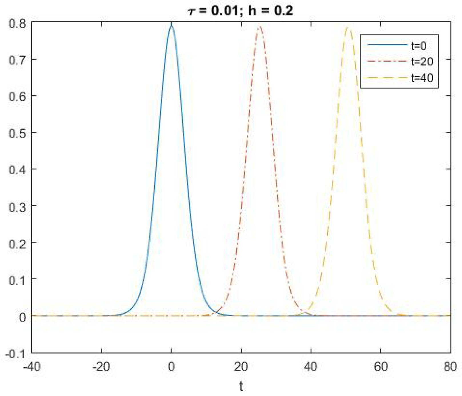
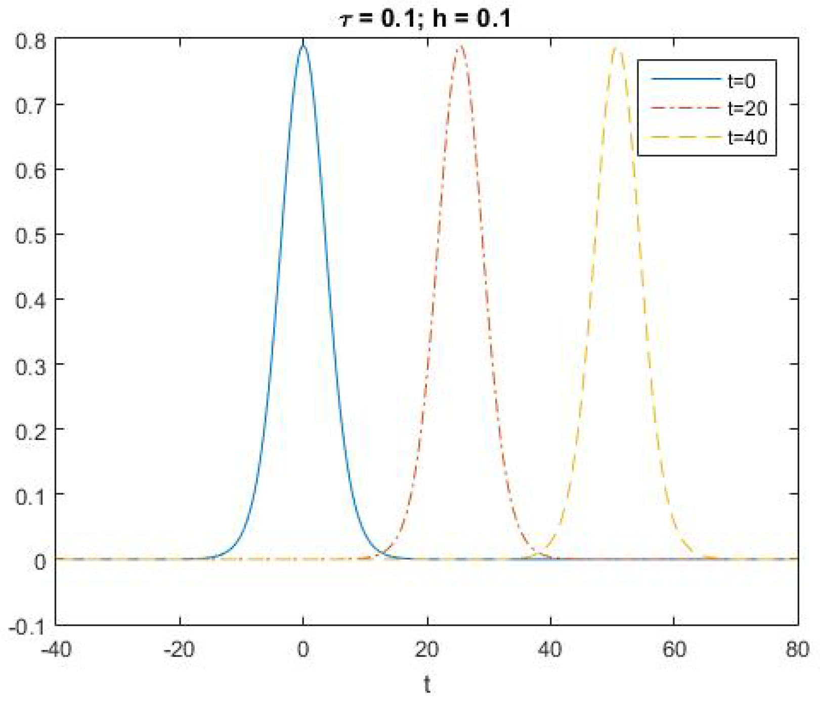
Next, the waveforms of $u(x,t)$ generated by scheme (12)–(14) with different $\tau$ and h are illustrated in Figure 1, Figure 2 and Figure 3. The waveforms at $t=20$ and 40 in Figure 1, Figure 2 and Figure 3 with different ratios of $\frac{\tau }{h}$ demonstrate a significant level of agreement with the waveforms at $t=0$, which also indicates the stability and the efficiency of scheme (12)–(14).

For various values of $\tau$ and h,

Table 1. The errors of the numerical solutions for the scheme (12)–(14).

	$\parallel \mathit{e}\parallel$			${\parallel \mathit{e}\parallel }_{\mathit{\infty }}$
	$\mathit{\tau }=\mathbf{0}.\mathbf{2}$	$\mathit{\tau }=\mathbf{0}.\mathbf{1}$	$\mathit{\tau }=\mathbf{0}.\mathbf{05}$	$\mathit{\tau }=\mathbf{0}.\mathbf{2}$	$\mathit{\tau }=\mathbf{0}.\mathbf{1}$	$\mathit{\tau }=\mathbf{0}.\mathbf{05}$
	$\mathit{h}=\mathbf{0}.\mathbf{2}$	$\mathit{h}=\mathbf{0}.\mathbf{1}$	$\mathit{h}=\mathbf{0}.\mathbf{05}$	$\mathit{h}=\mathbf{0}.\mathbf{2}$	$\mathit{h}=\mathbf{0}.\mathbf{1}$	$\mathit{h}=\mathbf{0}.\mathbf{05}$
$t=10$	6.7029 × ${10}^{-3}$	1.6805 × ${10}^{-3}$	4.2042 × ${10}^{-4}$	2.6525 × ${10}^{-3}$	6.6560 × ${10}^{-4}$	1.6653 × ${10}^{-4}$
$t=20$	1.2440 × ${10}^{-2}$	3.1213 × ${10}^{-3}$	7.8109 × ${10}^{-4}$	4.7213 × ${10}^{-3}$	1.1855 × ${10}^{-3}$	2.9670 × ${10}^{-4}$
$t=30$	1.7372 × ${10}^{-2}$	4.3612 × ${10}^{-3}$	1.0916 × ${10}^{-3}$	6.3893× ${10}^{-3}$	1.6058 × ${10}^{-3}$	4.0197 × ${10}^{-4}$
$t=40$	2.1849 × ${10}^{-2}$	5.4869 × ${10}^{-3}$	1.3735 × ${10}^{-3}$	7.8847 × ${10}^{-3}$	1.9813 × ${10}^{-3}$	4.9603 × ${10}^{-4}$

,

Table 2. Accuracy verification of the scheme (12)–(14).

	${\mathit{o}\mathit{r}\mathit{d}\mathit{e}\mathit{r}\mathit{l}}_2$			${\mathit{o}\mathit{r}\mathit{d}\mathit{e}\mathit{r}\mathit{l}}_{\mathit{\infty }}$
	$\mathit{\tau }=\mathbf{0}.\mathbf{2}$	$\mathit{\tau }=\mathbf{0}.\mathbf{1}$	$\mathit{\tau }=\mathbf{0}.\mathbf{05}$	$\mathit{\tau }=\mathbf{0}.\mathbf{2}$	$\mathit{\tau }=\mathbf{0}.\mathbf{1}$	$\mathit{\tau }=\mathbf{0}.\mathbf{05}$
	$\mathit{h}=\mathbf{0}.\mathbf{2}$	$\mathit{h}=\mathbf{0}.\mathbf{1}$	$\mathit{h}=\mathbf{0}.\mathbf{05}$	$\mathit{h}=\mathbf{0}.\mathbf{2}$	$\mathit{h}=\mathbf{0}.\mathbf{1}$	$\mathit{h}=\mathbf{0}.\mathbf{05}$
$t=10$	–	1.9959	1.9990	–	1.9946	1.9989
$t=20$	–	1.9948	1.9986	–	1.9937	1.9984
$t=30$	–	1.9940	1.9983	–	1.9924	1.9981
$t=40$	–	1.9935	1.9981	–	1.9926	1.9979

and

Table 3. Mass conservative quantity (15) for scheme (12)–(14).

	$\mathit{\tau }=0.2$	$\mathit{\tau }=0.1$	$\mathit{\tau }=0.05$
	$\mathit{h}=\mathbf{0}.\mathbf{2}$	$\mathit{h}=\mathbf{0}.\mathbf{1}$	$\mathit{h}=\mathbf{0}.\mathbf{05}$
$t=0$	7.590639955020484	7.590639955020483	7.590639955020486
$t=10$	7.590634665809471	7.590636068121576	7.590641816651537
$t=20$	7.590634945172798	7.590637353103019	7.590647235368987
$t=30$	7.590635182737761	7.590638486631225	7.590652070720461
$t=40$	7.590657869703787	7.590752977258113	7.590646799689627

present the errors of the numerical solution, the results of accuracy tests, and the discrete mass quantities at different times, respectively.

Both Pan et al. [13] developed a two-level nonlinear Crank–Nicolson finite difference scheme, while Fu et al. [31] proposed a pseudo-compact Crank–Nicolson conservative difference scheme that achieves comparable accuracy to the numerical scheme (12)–(14) presented in this paper. For clarity in comparison, we designate the compact scheme from [31] as Scheme I and the nonlinear scheme from [13] as Scheme II. Our comparative analysis focuses on these existing schemes and the proposed scheme (12)–(14). All numerical experiments were conducted with a fixed final time $T=20$. In

Table 4. Comparison of different finite difference schemes at $T=20$.

	Scheme I	Scheme II	Scheme (12)–(14)
$\tau =h=0.2$	3.6696 × ${10}^{-3}$	4.8122 × ${10}^{-3}$	4.7213  × ${10}^{-3}$
$\tau =h=0.1$	9.2056 × ${10}^{-4}$	1.2083 × ${10}^{-4}$	1.1855  × ${10}^{-3}$
$\tau =h=0.05$	2.3034 × ${10}^{-4}$	3.0242 × ${10}^{-4}$	2.9670  × ${10}^{-4}$
$\tau =h=0.025$	5.7597 × ${10}^{-5}$	7.5628 × ${10}^{-5}$	7.4285 × ${10}^{-5}$

, the ${\parallel ·\parallel }_{\infty }$ norms for absolute errors for various $\tau$ and h are listed. it can be seen that the proposed scheme (12)–(14) yields slightly smaller numerical errors than Scheme II and both schemes exhibit larger errors compared to Scheme I. The enhanced accuracy of Scheme I results from its compact stencil formulation, though this comes at the cost of increased computational expense and a longer runtime. Notably, our scheme achieves its superior performance relative to the nonlinear Scheme II while maintaining a linear structure—a particularly advantageous feature for practical implementations.

7. Conclusions

In this paper, a linearized difference scheme (12)–(14) for problem (4)–(6) is proposed, which can possess second-order theoretical accuracy both in the temporal and spatial directions. Compared with existing methods, the proposed linearized scheme not only avoids the computational complexity of nonlinear iterations inherent in the traditional Crank–Nicolson scheme but also preserves the mass conservation property of numerical solutions. Typically, conventional three-level linear schemes are not self-starting and require auxiliary methods to compute the initial values. In contrast, the proposed two-level scheme can eliminate this requirement.

Although in the current work, we only focus on the second-order accurate scheme, higher-order numerical schemes can be derived using higher-order Taylor expansions or other novel techniques [17,23,32]. Furthermore, extending this approach to construct similar linearized conservative difference algorithms for more complex models, such as the Rosenau–KdV–RLW equation and the Rosenau–Kawahara–RLW equation, will be the subject of our future research.

References

1. Peregrine, D.H. Calculations of the development of an undular bore. J. Fluid Mech. 1966, 25, 321–330. [Google Scholar] [CrossRef]
2. Peregrine, D.H. Long waves on a beach. J. Fluid Mech. 1967, 27, 815–827. [Google Scholar] [CrossRef]
3. Wazwaz, A.M. Analytic study on non-linear variants of the RLW and the PHI-Four equations. Commun. Nonlinear Sci. Numer. Simulat. 2007, 12, 314–327. [Google Scholar] [CrossRef]
4. Mohammadi, M.; Mokhtari, R. Solving the generalized regularized long wave equation on the basis of a reproducing kernel space. J. Comput. Appl. Math. 2011, 235, 4003–4014. [Google Scholar] [CrossRef]
5. Rosenau, P. A quasi-continuous description of a nonlinear transmission line. Phys. Scr. 1986, 34, 827–829. [Google Scholar] [CrossRef]
6. Rosenau, P. Dynamics of dense discrete systems: High order effects. Prog. Theor. Phys. 1988, 79, 1028–1042. [Google Scholar] [CrossRef]
7. Kim, Y.D.; Lee, H.Y. The convergence of finite element Galerkin solution for the Rosenau equation. Korean J. Comput. Appl. Math. 1998, 5, 171–180. [Google Scholar] [CrossRef]
8. Chung, S.K.; Pani, A.K. Numerical methods for the Rosenau equation. Appl. Anal. 2001, 77, 351–369. [Google Scholar] [CrossRef]
9. Hu, J.S.; Wang, Y.L. A high–accuracy linear conservative difference scheme for Rosenau–RLW equation. Math. Probl. Eng. 2013, 2013, 870291. [Google Scholar] [CrossRef]
10. Pan, X.T.; Zheng, K.L.; Zhang, L.M. Finite difference discretization of the Rosenau–RLW equation. Appl. Anal. 2013, 92, 2590–2601. [Google Scholar] [CrossRef]
11. Zuo, J.M.; Zhang, Y.M.; Zhang, T.D.; Chang, F. A new conservative difference scheme for the general Rosenau-RLW equation. Bound. Value Probl. 2010, 2010, 516260. [Google Scholar] [CrossRef]
12. Wang, H.; Li, S.G.; Wang, J. A conservative weighted finite difference scheme for the generalized Rosenau–RLW equation. Comput. Appl. Math. 2017, 3, 63–78. [Google Scholar] [CrossRef]
13. Pan, X.T.; Zhang, L.M. On the convergence of a conservative numerical scheme for the usual Rosenau–RLW equation. Appl. Math. Model. 2012, 36, 3371–3378. [Google Scholar] [CrossRef]
14. Wongsaijai, B.; Poochinapan, K. A three-level average implicit finite difference scheme to solve equation obtained by coupling the Rosenau–KdV equation and the Rosenau–RLW equation. Appl. Math. Comput. 2014, 245, 289–304. [Google Scholar] [CrossRef]
15. Wongsaijai, B.; Mouktonglang, T.; Sukantamala, N.; Poochinapan, K. Compact structure-preserving approach to solitary wave in shallow water modeled by the Rosenau–RLW equation. Appl. Math. Comput. 2019, 340, 84–100. [Google Scholar] [CrossRef]
16. Wongsaijai, B.; Poochinapan, K. Optimal decay rates of the dissipative shallow water waves modeled by coupling the Rosenau–RLW equation and the Rosenau–Burgers equation with power of nonlinearity. Appl. Math. Comput. 2021, 405, 126202. [Google Scholar] [CrossRef]
17. Pan, X.T.; Wang, Y.J.; Zhang, L.M. Numerical analysis of a pseudo–compact C–N conservative scheme for the Rosenau–KdV equation coupling with the Rosenau–RLW equation. Bound. Value Probl. 2015, 2015, 65. [Google Scholar] [CrossRef]
18. Ghiloufi, A.; Omrani, K. New conservative difference schemes with fourth–order accuracy for some model equation for nonlinear dispersive waves. Numer. Methods Partial. Differ. Equ. 2018, 34, 451–500. [Google Scholar] [CrossRef]
19. Atouani, N.; Omrani, K. Galerkin finite element method for the Rosenau–RLW equation. Comput. Math. Appl. 2013, 66, 289–303. [Google Scholar] [CrossRef]
20. Karakoc, S.B.G. A new numerical application of the generalized Rosenau–RLW equation. Sci. Iran. 2020, 27, 772–783. [Google Scholar] [CrossRef]
21. Shi, D.; Jia, X. Superconvergence analysis of a mixed finite element approximation for the nonlinear fourth–order Rosenau–RLW equation. Comput. Math. Appl. 2021, 98, 169–180. [Google Scholar] [CrossRef]
22. Kutluay, S.; Karta, M.; Uçar, Y. Strang time–splitting technique for the generalised Rosenau–RLW equation. PRAMANA-J. Phys. 2021, 95, 148. [Google Scholar] [CrossRef]
23. Mustahsan, M.; Kiran, A.; Singh, J.; Nisar, K.S.; Kumar, D. Higher order B–spline differential quadrature rule to approximate generalized Rosenau–RLW equation. Math. Method. Appl. Sci. 2020, 43, 6812–6822. [Google Scholar] [CrossRef]
24. Guo, C.; Li, F.; Zhang, W.; Luo, Y. A conservative numerical scheme for Rosenau–RLW equation based on multiple integral finite volume method. Bound. Value Probl. 2019, 2019, 168. [Google Scholar] [CrossRef]
25. Ghiloufi, A.; Kadri, T. Analysis of new conservative difference scheme for two-dimensional Rosenau–RLW equation. Appl. Anal. 2017, 96, 1255–1267. [Google Scholar] [CrossRef]
26. Li, S.G. Numerical analysis for fourth–order compact conservative difference scheme to solve the 3D Rosenau–RLW equation. Comput. Math. Appl. 2016, 72, 2388–2407. [Google Scholar] [CrossRef]
27. Wang, X.F.; Dai, W.Z.; Yan, Y. Numerical analysis of a new conservative scheme for the 2D generalized Rosenau–RLW equation. Appl. Anal. 2021, 100, 2564–2580. [Google Scholar] [CrossRef]
28. Tamang, N.; Wongsaijai, B.; Mouktonglang, T.; Poochinapan, K. Novel algorithm based on modification of Galerkin finite element method to general Rosenau–RLW equation in (2+1)–dimensions. Appl. Numer. Math. 2020, 148, 109–130. [Google Scholar] [CrossRef]
29. Zhou, Y.L. Application of Discrete Functional Analysis to the Finite Difference Method; International Academic Publishers: Beijing, China, 1990. [Google Scholar]
30. Zheng, K.L.; Hu, J.S. High–order conservative Crank–Nicolson scheme for regularized long wave equation. Adv. Differ. Equ. 2013, 2013, 287. [Google Scholar] [CrossRef]
31. Fu, Y.Z.; Hu, B.; Zheng, M.B. Pseudo–compact Crank–Nicolson conservative difference scheme for Rosenau-RLW equations. J. Sichuan Univ. (Nat. Sci. Ed.) 2014, 51, 1143–1148. (In Chinese) [Google Scholar]
32. Clainche, S.L.; Vega, J.M. Higher order dynamic mode decomposition. SIAM J. Appl. Dyn. Syst. 2017, 16, 882–925. [Google Scholar] [CrossRef]
Figure 1. Numerical solutions of u ( x , t ) with τ = 0.2 , h = 0.01 .
Axioms 14 00395 g001
Figure 2. Numerical solutions of u ( x , t ) with τ = 0.01 , h = 0.2 .
Axioms 14 00395 g002
Figure 3. Numerical solutions of u ( x , t ) with τ = 0.1 , h = 0.1 .
Axioms 14 00395 g003