Abstract
Mobile robots are extensively utilized across various fields, with path planning consistently representing a core and pivotal area of research. Path planning is essential for enabling the efficient navigation of robots within complex environments. In reality, the terrain on which the robot operates is non-uniform, resulting in varying costs associated with different areas due to differing terrains and materials. Practical tasks often necessitate traversing a series of landmark points to fulfill specific requirements. Furthermore, considerations related to control and dynamics frequently require setting minimum line segment lengths between curves and maximum curve curvatures to ensure the successful execution of the path. The objective of this paper is to find a low-cost path with continuous curvature on a map with an assigned cost, which passes through all the given landmark points while avoiding obstacles, and satisfies the minimum length of the line segments between the curves and the maximum curvature constraints of the curves. We propose an innovative path planning method that solves the limitations of traditional algorithms by considering map cost, curvature continuity, and other factors by establishing a collaborative mechanism between global coarse search and local fine-tuning. The method is divided into two stages: In the first stage, the graph structure is constructed by generating points on the map, and uses Dijkstra’s Algorithm to obtain the connection order of the landmark points. In the second stage, which builds on the previous stage and processes landmark points sequentially, the key points of the path are generated using our proposed Smooth Beacon Reconnection (SBR) algorithm. A low-cost path meeting the requirements is then obtained through fine-tuning. The smooth path generated by this method is verified on multiple maps and demonstrates superior performance compared to traditional methods.
Keywords:
mobile robot; path planning; mathematical modeling; continuous curvature; map costs; landmark points MSC:
00A69; 90-10; 90C90
1. Introduction
With the rapid advancement of science and technology, robotics has become widely applicable in various fields, including industrial automation, the service industry, and medical assistance. Robot navigation, which underpins autonomous movement and task execution, remains a core focus within robotics. Path planning is a critical component of robot navigation, addressing the design of an optimal and effective route for robots to travel from a starting point to a destination within complex environments. Effective path planning enhances mobility efficiency, ensures safety, and reduces energy consumption.
In the real world, the terrain where path planning occurs is often non-uniform. Different terrains and materials result in varying costs for the same distance traveled by a robot. For instance, the robot pays a higher cost when passing through terrain with water than when passing through smooth terrain. Additionally, due to specific task requirements and the robot’s motion characteristics, the generated path must adhere to several constraints and be sufficiently smooth to avoid additional costs and risks. In practical applications, robots often need to traverse a series of landmark points to fulfill specific requirements, such as picking up goods or refueling. Due to system control and dynamic factors, short line segments between curves can introduce excessive turns, complicating control and making it difficult to manage acceleration, deceleration, or steering. This can amplify errors, causing the path to deviate from the target and incurring additional costs and risks. Referring to Figure 1, we divide the line segments between the curves into two categories for discussion, namely the co-direction curves and the reverse curves. Similarly, if the maximum curvature of the curve is not limited, when the robot exceeds the maximum curvature limit that the steering system can withstand, it will not only deviate from the route but also cause wear and tear of the equipment. To ensure the path’s feasibility, we impose constraints on the minimum length of line segments between curves and the maximum curvature of the curves while the path is reasonable. The goal of this paper is to find a low-cost, curvature-continuous path on a cost-assigned map that passes through all given landmark points, avoids obstacles, and satisfies the constraints of the minimum length of line segments between curves and the maximum curvature of the curve.
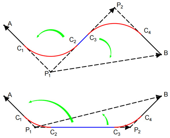
Figure 1.
Minimum length of line segments between curves.
Classic path planning algorithms, such as Dijkstra’s Algorithm and A*, are effective in many cases but typically assume that the path is composed of straight segments, without considering path curvature. Methods that use splines to generate a smooth path, like Bezier curves, may not always align with the robot’s motion characteristics and rely on added control points to meet the obstacle avoidance requirements, leading to potential route deviations and errors. Line segments and circular curves offer significant advantages in path planning, facilitating easier control and smoother turns for robots, reducing wear and tear, and maintaining stability. A clothoid is a curve with continuously changing curvature. Its predominant characteristic is that the curvature of a point on the curve is proportional to the distance moved along the curve to that point. This design helps robots better follow the predetermined path, enhancing accuracy, work efficiency, and precision while minimizing control errors from sudden curvature changes. This paper explores a novel path planning method through mathematical modeling to generate a smooth path that better aligns with actual task requirements and the machine’s motion characteristics while considering costs. We first define a mathematical model that meets specific needs and constraints, and based on this, propose a two-stage algorithm. In the first stage, the graph structure is constructed by generating points on the map, and we use Dijkstra’s Algorithm to obtain the connection order of the landmark points; the second stage builds on the previous stage and deals with landmark points one by one, and then the key points of the path are generated by using the Smooth Beacon Reconnection (SBR) algorithm proposed by us. Finally, the low-cost path that meets the requirements is obtained after fine tuning.
This study makes significant contributions in the following aspects:
- Addressing the limitation of traditional algorithms that fail to consider walking costs associated with terrain and materials, our proposed algorithm is capable of generating an economically viable route on a cost map.
- Overcoming the drawbacks of conventional algorithms where smooth paths comprise multiple smooth paths, our algorithm seamlessly transitions between line segments and arcs through the clothoid to ensure overall path curvature continuity.
- The proposed mathematical model considers the dynamic factors of the robot and the accuracy requirements of system control, incorporating constraints such as the minimum length of line segments between curves and the maximum curvature of the curve.
- The algorithm we propose takes into consideration real task landmark points and obstacle avoidance requirements, ensuring that the path passes through all specified points while avoiding obstacles. Experimental evaluations are conducted on maps in various common scenarios to assess its performance.
- Through comparison with traditional researches, it is evident that the new method closely aligns with real-world needs, demonstrating its superiority in smooth path planning.
This paper consists of six sections, which is arranged as follows: In Section 2, we review the related work, including the research progress of traditional path planning algorithm and smooth path. In Section 3, we first introduce the basic concept of clothoid and some basic constraints of the problem, then give a method of completing the transition between line segment and arc through clothoid, and finally put forward the mathematical model of the problem studied in this paper. Section 4 describes the proposed two-stage algorithm based on global coarse search and local optimization, thereby achieving the decoupling solution of decision-making and geometric constraints for the problem. Section 5 describes the experimental environment, explains the experimental parameters, and further proves the rationality and efficiency of the algorithm through the analysis results. In the last Section 6, we summarize the paper, point out the deficiencies of the current work and give the direction of future work.
2. Related Work
Path planning (PP) is gradually becoming more crucial in the field of autonomous mobile robots. So far, many algorithms have been used to solve this problem. The algorithm proposed by Dijkstra E.W. [1] is one of the classic algorithms. It continuously updates the shortest path distance between the node and the starting point to find the shortest path; The A* algorithm [2] uses a heuristic function that combines the actual cost and the estimated cost to measure the cost to the target node, and gives priority to low-cost nodes during the search process. These two methods lack curvature continuity, rendering them unsuitable for robot control where abrupt directional changes induce instability and mechanical wear. Building upon the A* algorithm, Sun et al. [3] enhanced its efficiency by reducing unnecessary operations on the open list, yet their approach still inherits these limitations. Harabor and Grastien [4] proposed the JPS algorithm which expands the points added to the OpenList based on the strategy of searching for jump points, aiming to optimize the operation of searching for successor nodes. Their work can place the map cost within the graph structure, but ignores the curvature constraints. The algorithm proposed in this paper integrates the advantages of the classical graph search algorithms, such as fast running speed and cost consideration, and generates smooth paths that meet the conditions by finding key points.
Different from the graph search algorithm running on a given graph structure, the Sampling-Based Planning (SBP) algorithm also widely used due to its property of probabilistic completeness, i.e., a solution will be provided, if one exists, given infinite runtime [5,6]. The most classic algorithm is the RRT algorithm proposed by LaValle S. [7], which searches for paths by randomly sampling in space and gradually building a tree structure. Based on the RRT algorithm that searches for path by randomly sampling in space and gradually constructing a tree structure, the RRT* algorithm proposed by Karaman and Razzoli [8] enhances the path quality through rewiring and neighborhood search, and proves the asymptotic optimality of the algorithm, but there may be no solution in the short time; Nasir et al. [9] improved the convergence speed of this algorithm through intelligent sampling and path optimization. Faroni et al. [10] proposed an adaptive hybrid sampling strategy that regulates the trade-off between local and global information. The performance, however, may exhibit significant variability contingent upon the problem’s geometry and the selected parameters. DG-RRT proposed by Huang et al. [11] enhances efficiency by incorporating a dynamic gradient sampling strategy that concentrates guide points toward the goal region and employs a root-node iterative optimization method to refine paths. However, if the landmark points that a path must approach are involved, there guiding confusion will occur. The method proposed in this paper takes this problem into consideration. Although these sampling-based methods can produce more flexible paths compared to graph-based approaches, their performance can be highly variable depending on the sampling strategy and environmental complexity; additionally, the cost of the map is not taken into consideration. The proposed algorithm in this paper integrates the exploration of the global situation through sampling, and retains the cost information of the map by constructing the graph structure, using Dijkstra’s Algorithm to quickly generate the detection path.
Heuristic algorithms are widely used in path planning because of their high efficiency and flexibility. For example, the genetic algorithm optimizes the solution of a problem by simulating the process of natural selection, while particle swarm optimization finds the optimal solution by simulating the predation behavior of birds; other examples include simulated annealing, tabu search, and so on. To address the drawbacks of traditional ant colony optimization (ACO) algorithms, Miao et al. [12] developed an enhanced algorithm (IAACO) for mobile robot path planning in an enclosed area. IAACO introduces angle guidance factors and obstacle exclusion factors to enhance safety in path planning, but it lacks a systematic evaluation regarding efficiency in diverse scenarios. The algorithm proposed in this paper has been verified in multiple scenarios. Cai et al. [13] improves the ACO algorithm by integrating it with the firefly algorithm and heuristic functions, leading to enhanced performance in path planning for different environments. However, the performance is still heavily reliant on initial parameter selection and may not completely avoid local optima or oscillations in complex environments. While these methods demonstrate distinct advantages across various application scenarios, their lack of curvature constraints and other limitations make them challenging to implement directly in practical robot motion control systems.
In terms of smooth path planning, Kanayama and Hartman [14] used two types of simple path sets to solve the path planning problem of symmetrical postures according to the defined smooth path cost, but there are problems such as discontinuous curvature. The algorithm combined with parameter curve smoothing scheme also has good performance. Most RRT-based extension algorithms can generate safe and smooth paths by combining parameter curve-based smoothing schemes. A path planning algorithm for a non-holonomic robot proposed by Fei et al. [15] integrates cubic Bézier splines with Informed RRT. The algorithm ensures curvature continuity and kinematic constraints but increases computational complexity. Yang et al. [16] proposed a Bezier curve-based algorithm to check the local smoooth path before each random tree expansion, ensuring smoothness and safety. Similar to this is Elbanhawi et al. [17]’s C2 continuous algorithm based on a B-spline curve. However, these do not take into account factors such as the cost of the map and landmark points that the path must approach. The algorithm proposed in this paper considers these problems through strategies such as graph structure and point-by-point detection. Li et al. [18] proposed a global path planning method based on the bidirectional alternating search strategy A* algorithm. This approach involves alternating searches for path nodes, utilizing Bezier curves to achieve path smoothing and introducing a path node filtering function to reduce redundant nodes. The algorithm effectively addresses the smooth path planning problem; however, it may still exhibit long computation times on large-scale maps, and its robustness in complex environments requires further verification. Liao et al. [19] proposed the Stack-RRT* algorithm to generate the paths with varying continuity levels, which integrates with diverse parameterized curve smoothing schemes; Huang H.-C. [20] used the parallel PSO algorithm to find a feasible route and then used cubic B-spline to smooth the route. These two methods rely heavily on the initial direction and the initial solution. The algorithm proposed in this paper effectively avoids this limitation. Bakdi et al. [21] used a genetic algorithm to obtain an obstacle avoidance path, and then used piecewise cubic hermite interpolation polynomials to generate a smooth path without considering the maximum curvature. Song et al. [22] combined Bezier curves with genetic algorithms, set the control points at the center of the grid, and the resulting smooth path was unable guarantee the curvature continuity at the connection points. Lin et al. [23] solved the problem above by combining cubic Bezier curves with an adaptive delayed velocity particle swarm algorithm, which has equivalent curvature at the curve connection, thereby ensuring the smoothness and continuity of the entire path, but it does not consider that it is necessary for the robot to adjust avoiding deviating from the route. Saurabh and Ashwini [24] present a path planning method using four-parameter logistic curves for continuous-curvature paths with obstacle avoidance, providing analytic solutions for generating smooth paths that avoid both rectangular and circular obstacles.
Existing approaches often overlook the actual situation, including critical factors such as the robot’s kinematic constraints and dynamic limitations. This omission may result in deviations from the intended path, introducing risks like control instability, mechanical wear, or unintended collisions during execution. The algorithm we proposed finds a low-cost path on a map with cost, and it has continuous curvature, avoids obstacles, passes through all given landmark points, and satisfies the minimum length of line segments between curves and the maximum curvature constraints of the curve.
3. Problem Formulation and Model
3.1. Preliminary on Clothoid
The term clothoid denotes a curve characterized by a smoothly varying curvature, transitioning between a straight line and a circular arc, or between two circular arcs in a planar configuration. Its main characteristic is that the curvature of a point on the curve is proportional to the distance moved along the curve; that is, its curvature changes linearly with the length of the curve, which ensures that the machine’s uniform steering wheel rotation is consistent with the transition trajectory of the straight line and the circular curve. A clothoid curve can be uniquely determined by the following parameters: 1. The length of clothoid L. 2. The coordinates and heading angle of the starting point . 3. The two parameters that determine its linear curvature function. Given these parameters, we can calculate the position and heading angle of the curve at any point t in by solving the following (Equation (1)):
If is equal to 0, according to the properties of the clothoid, the product of the radius of curvature r at any point on the curve and the length of the curve s at that point is a constant, denoted as . When , according to the geometric relationship, it can be seen that the center angle corresponding to the curve between any point on the clothoid and its starting point is the tangent angle, which is the angle between the tangent line of the point and the starting point tangent line, referring to the left figure of Figure 2. Take a differential arc segment at any point, and the corresponding center angle is , so there is
thus,
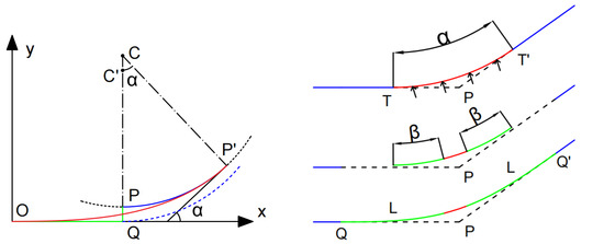
Figure 2.
Clothoid inserted between line segment and arc.
Integrating the Equation (3) on both sides of the equal sign, respectively, and according to the initial conditions, we obtain the following:
further, we can obtain
that is
On this basis, we can obtain the following:
the series expansion formulas for and , respectively, are as follows:
It follows that
Obviously, through the Root test, and converge absolutely.
3.2. Landmark Points and Minimum Line Length Limit
In some tasks, a series of landmark points are required to meet the task requirements, such as delivery robots picking up goods, refueling, etc. In addition, setting landmark points manually can also help avoid obstacles on the map in complex environments and reduce path costs.
Regarding the issue of line segment length, in some application scenarios, such as robot movement or vehicle driving, if the line segments are too short it may introduce excessive turns or transformations, resulting in inaccurate control or execution, which may amplify errors and cause the path to deviate from the target. In numerous road design scenarios, the establishment of a minimum line length between curves is crucial for preserving the continuity of the line shape and guaranteeing the practicality and implementability of the route. For mobile robots, cars or other vehicles, kinematic constraints usually require acceleration, deceleration or turning within a certain minimum distance. It can be ensured that these kinematic constraints are satisfied by setting the minimum length of a straight line segment.
We divide the minimum line segment length into two cases for discussion, namely, the line segment length constraint between the same-direction curve and the reverse-direction curve, as shown in Figure 1. For a two-dimensional plane, let , . Determine the direction based on the vector cross product property. If , then point A is on the left side of . Similarly, the calculation of point B can determine whether point A and point B are on the same side.
3.3. A Smooth Transition Between Line Segment and Arc
Line segments and circular curves have very significant advantages in route planning. Line segments make it easier to control the robot, and circular curves can provide smooth turns. Both of them can reduce the emergency stops and turns of the robot during movement, which is important for maintaining the stability of the robot. Robot stability and reducing mechanical wear are very beneficial. However, directly using line segments and circular curves does not ensure that the route curvature is continuous. In this case, the clothoid needs to be inserted between the two to achieve a smooth transition.
As shown in the left image of Figure 2, the red represents the clothoid and the blue represents the arc, with the line segment tangent to the arc at point Q, and the radius of the dotted arc is equal to ; the radius of the solid arc is R. We can insert a clothoid curve of length L between the line and solid arc; that is, the red curve in the figure. For ease of processing, assume that the starting point of the clothoid curve is at the origin and the initial heading angle is 0. From the above, we obtain . Assuming , we can calculate the value of , , and their convergence characteristics through geometric analysis, combined with the application of Formula (9). The values of and are functions of , recorded as and , respectively.
The right image of Figure 2 shows the method of smoothly transitioning the line type combination of ‘’. Assume that the center of the arc is point C, the radius is R, the central angle is , and it is tangent to the line segments at points . The extended lines of the line segments intersect at point P. The radius of the arc decreases by units. At this time, the distance from point P to C is . The central angle is reduced from both ends by , resulting in the processed arc; points are moved along by units to obtain points as the starting points of clothoid, so that the smooth transition between the line segment and the arc is completed by inserting the clothoid. Obviously, this method causes the calculation radius of the arc to change. In order to keep the calculation radius unchanged, after obtaining the tangent point, move units distance in the opposite direction of point P to obtain point Q corresponding to the left image of Figure 2. The center of the circle is point . After moving a distance of along the direction and then reducing the angle, the coordinates of clothoid and arc connection are obtained. It should be noted that the same treatment should be carried out at both ends.
From the right image of Figure 2, it is clear that is required to complete the transition successfully. This method is particularly suitable for highway design and other path planning scenarios, where the curvature of the route is moderate and the path is required to be smooth and efficient.
By setting a reasonable length of clothoid, not only can the sudden load on the actuator be reduced and wear minimized, but it also enables the mobile robot to navigate turns in the path at a speed closer to the expected velocity, thereby enhancing task completion efficiency. We know that the centrifugal acceleration is generated by the centrifugal force. If the length of the clothoid curve from the straight part to the arc part of the robot is L, and the radius at the end point is R, then the centrifugal acceleration increases uniformly from 0 to , and the centrifugal acceleration change rate . Then, . In Crausd’s research [25], the centrifugal acceleration change rate of route design is usually set to 0.3–0.9. The larger the centrifugal acceleration change rate, the shorter the curve length, and the easier it is to complete the insertion. Different robots have different design parameters and motion requirements, so the value of is different, but it is a fixed constant. The research content of this paper requires that the curvature is continuous, so setting the eccentricity acceleration value to 0.4 and the speed parameter to 2 does not affect the overall calculation and algorithm effect.
3.4. Model
We now describe the problem to be solved in detail. According to the given cost map, find a smooth path connecting the starting point and the ending point, where the smooth path should meet the following optimization criteria and constraints: 1. Pass through all given landmark points; 2. Avoid given obstacles; 3. The path meets the requirement of curvature continuity; 4. Due to the design of the robot, the path has a maximum curvature limit, that is, there is a minimum radius limit for the arc; 5. The length of the line segment between the curves is greater than the minimum length of the line segment of this type; 6. Under the above criteria and constraints, reduce the cost of the path. Then, the optimization problem we proposed is formulated as follows:
Here, represents the function that assigns the map cost, supposed to be a reasonable non-negative function with an upper bound; represents the arc in the curve set C with radius under the key points and the corresponding clothoid, and represents the line segment under the key points and the radius of the adjacent arc in the line segment set L. Then, we further explain the model in combination with Figure 3.
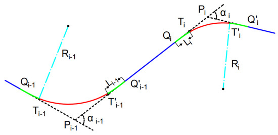
Figure 3.
Path generation method and constraints.
As shown in Figure 3, the red parts in the figure are arcs, the green parts are clothoids, and the blue parts are line segments. It is obvious that the degree of each angle and the number of curves are uniquely determined by the key point set P. Here, the point of tangency between the arc and the line segment before the clothoid curve is inserted is represented by T, Q is the connection point between clothoid and the line segment, R represents the radius of the corresponding circular curve, the length of clothoid is represented by L, and according to Formula (11), represents the outward displacement value of the tangency point, while represents the distance between the key point and the tangent point before insertion. We assume that both the starting point and the ending point are passed by line segments, that is, ; then, the number of line segments is one more than the number of curves. represents the route generated by the sets C and L. Formula (12) minimizes the cost of the route on the map under the control of the point set P and the arc radius set R. Among them, represents the cost of the curve part of the path, and represents the cost of the straight part of the path. Formula (13) indicates that the generated path should satisfy curvature continuity, and Formula (14) represents the path in the feasible area of the map. Formula (15) indicates that the path needs to pass through all given landmark points, where is the set of landmark points. According to the content of Section 3.3, it can be known that the curvature of the inserted clothoid is between 0 and the arc curvature. Therefore, the maximum curvature of each curve part is the arc curvature of that curve part. The maximum curvature corresponds to the minimum arc radius, so Formula (16) represents that the route has a maximum curvature restriction. From the above text, represents the distance between the key point and the starting point of clothoid. Therefore, Formula (17) represents that the length of the line segment has a minimum length constraint.
When the key points are determined, the z value of each line segment is uniquely determined, according to Section 3.2. As can be seen from Section 3.3, Formula (18) ensures that the clothoid can be smoothly inserted into the arc.
4. Algorithm
We propose a two-stage algorithm. In the first stage, the graph structure is constructed by generating points on the map, and we use Dijkstra’s Algorithm to obtain the connection order of the landmark points; in the secondary stage, the Smooth Beacon Reconnection (SBR) algorithm proposed by us is used to find the key points of the path, and the low-cost path that meets the requirements is obtained after fine tuning.
The algorithm flow chart is shown in Figure 4, and the algorithm pseudo-code Algorithm 1 is also shown. The input data include parameters, landmark points (including the starting and ending points), the boundary, obstacles, and the map cost function , among which the last four are the necessary elements of the map (). In Figure 4, the data flow along the dotted line, and the algorithm process is represented by the solid line. The parameters include the upper limit of the number of generating points N, the control time T, and the control distance . By default, ; this is because according to the rule of taking points, there must be . Here, we take the nearest smallest integer 4, and the incremental cost threshold is 1. Since doubling the cost is considered significant, if this value is too large, it may cause the algorithm to be insensitive to high-cost regions. If it is too small, it will be overly sensitive, leading to the failure of the algorithm or even no solution. Some parameter selections are related to information, such as the map. The parameters selected in this paper can refer to Section 5.2.
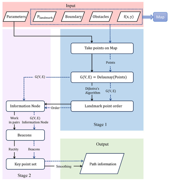
Figure 4.
Algorithm flow chart.
The first line initializes the map information point set and puts all the landmark points into the set, setting the number of counts to 0; lines 2–16 take points from the map. If a random point on the map satisfies that the distance to all points in the set is greater than , then the point is added to the set. The effect after generating the points is shown in Figure 5, where the green points are the landmark points; the 17th line generates a graph structure based on the Delaunay triangulation according to the point set. Up to this line of the algorithm, the time complexity is , and the space complexity is , in which n is the number of points. The effect is shown in Figure 6. The weight of any side in is the line integral of its map cost function . The Delaunay triangulation is selected as the basic graph structure because it can more effectively represent the irregular characteristics of map cost than other structures such as grids.
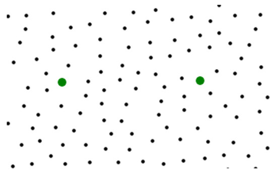
Figure 5.
Random points on the map.
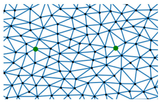
Figure 6.
Delaunay triangulation network constructed as G.
Assuming the number of points of the graph is n, according to Euler’s Formula of the plane
where and represent the number of edges and faces, respectively. Each triangle has three edges, and each edge is shared at most by two triangles, so . The simultaneous solution gives the following:
When the case of the graph structure boundary is not considered, that is, each edge is shared by two triangles, it follows that
That is, the number of edges increases linearly with the number of points:
Similarly, in the grid graph, the following is the case:
and then
In the case of the same number of points, the Delaunay triangle-based graph has more edges and can cover more information.
The next step needs to determine the connection order of the landmark points, which corresponds to line 18 of the pseudo-code. As shown in Figure 7, the cost between two landmark points is determined by the shortest distance determined by Dijkstra’s Algorithm on the graph . As shown in Figure 8, a Hamiltonian circuit is constructed by adding a virtual node, where the distance from the virtual point to the starting point and ending point is 0, and the distance from other nodes is infinite. This Hamiltonian circuit can determine the connection order of each landmark point. The red point in the figure is the virtual point, while the green points represent the starting and ending points, and the blue points serve as landmark points, thus completing the first step of the algorithm. Up to this line, Algorithm 1 resolves the issue of connection order among landmark points.
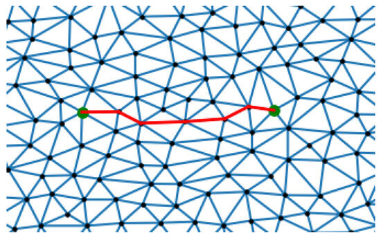
Figure 7.
Shortest path between two points as cost.
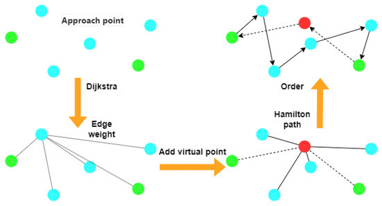
Figure 8.
Determination of the approach point order.
The second step of the algorithm sees the 19th and 20th lines of Algorithm 1. The connection order of the landmark points obtained in the first stage are processed one by one. The pseudo-code of the algorithm in the 19th line is shown as Algorithm 2 Smooth Beacon Reconnection , where the first line initializes the set of information nodes and key points. From the second line to the seventh line, new information nodes are obtained as part of the key points, and the fourth line indicates that the landmark point is transitioned in the form of a line segment according to the trend of the landmark points. The use of a line segment rather than a curve for the transition is because a line segment is better suited to real-world needs, such as picking up goods or refueling.
| Algorithm 1 Smooth path search based on two stages |
Input:
|
Figure 9 shows the generation of the trend according to the connection order, the dotted line represents the connection order, and the solid line represents the direction trend generated by the connection order. The blue dot represents the landmark point being processed, and the green dots represent the two landmark points before and after it. Figure 10 shows the transition of the landmark point with line segments; that is, two key points are generated in the trend direction, where the direction of the trend line is controlled by the position of obstacles and the length of the line segment. The blue dot is the processed landmark point, and the green dots represent the two landmark points before and after it. When the original direction leads to obstacles in the way, the direction will be adjusted. And the parameter of the length of the line segment is determined by the minimum line segment length and the maximum curvature in the constraint.
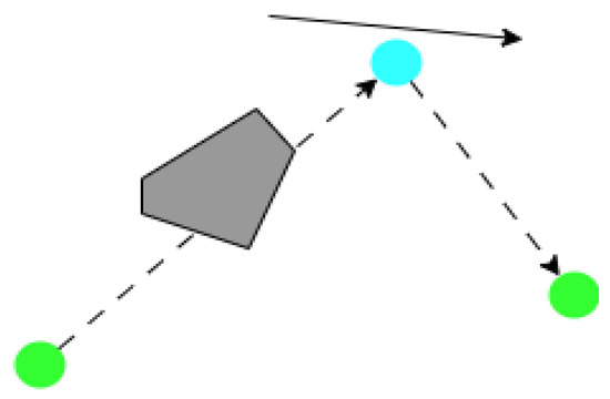
Figure 9.
Trend is identified by order.
Figure 10.
Transition through line segment.
The specific practices are as follows: If the order is determined, the connection order of three landmark points is , , and . The middle point is transitioned by passing through a line segment. The direction of the line segment is . Based on the assumption that all landmark points complete the transition through the line segment, two information nodes are generated by one landmark point in the trend direction, where the direction of the trend line is controlled by the position of the obstacle and the length of the line segment. For example, the direction will be adjusted when the original direction causes obstacles in the path; the adjustment method takes the landmark point as the center and swings the trend line until the transition line segment does not pass through the obstacles, generally within debugging. The line length parameter is determined by the minimum line length and maximum curvature in the constraint, and is generally set to , which ensures that the constraints are satisfied after smoothing. This is because after removing the length of the of the constraint here, the maximum distance from each key point to the starting point of clothoid after being inserted into the curve is . Through Section 3.3, we know that this value is . Combined with the content from Section 3.1, we have the following:
Therefore, we should ensure that
It is generally believed that an angle greater than at each key point is in line with practical significance. A larger angle makes the path more gentle. In Section 5.2, we set the maximum curvature to 0.2 and the minimum value of the minimum line segment length between the curves to 2. Therefore, Formula (26) has a solution. More generally, the minimum value of the minimum line segment length between curves is set to . The end of this step adds the information nodes to and the set of information nodes is
The algorithm starts from line 8 to find key points in groups of two information nodes. At this time, each group of end points is connected by line segments in line 4 of the algorithm. Lines 10 and 18 indicate that the information nodes from the previous step are added to key points . The shortest path Localpath on the map is generated by Dijkstra’s Algorithm. Then, in lines 12 to 17, the points are methodically checked from the start to the end in the group. The reason why each node is set as the beacon first is that the point detected at this time may not necessarily be smoothed as a key point. Line 13 indicates that when the calculation is made in the form of a line segment, if the cost increases significantly, the increment exceeds the set threshold of the original cost times; then, the preceding node of the check node is set as a beacon node and a new starting point at the same time, and the checking of each point is continued until the end. If the value of is 0, then every point on Localpath becomes a beacon node.
The specific practices are as follows: If the starting point is S and the ending point is E, the landmark points are , , and in the connection order. After the transition of the previous step, the landmark points are connected in line segments at this time. The current node order is as follows: S, , , , , , , E. Among them, , , , , , are information nodes. The number of all information nodes is . The 2 indicates that there is a starting point and ending point, and indicates the number of landmark points. Since each landmark point generates two information nodes, the total number must be an even number. Now the grouping is as follows: , , , ; the beacon point can be searched for by line check calculation.
Figure 11 shows the process of finding key points. The gray area represents the high-cost area or prohibited area, the red dotted line represents the check node with increased cost after inspection, and the red solid line represents the result after inspection. Line 19 of Algorithm 2 calculates whether the current key point meets the smoothing generation conditions and whether it passes through the forbidden area after generation. If not, adjustments will be made, such as moving backward along the direction of the obstacle to generate the key point, as shown in Figure 12. It can be seen that the focus of the second stage is to find a beacon to turn the key point. After the curve insertion is completed, the generated path satisfies all the constraint conditions.
| Algorithm 2 SBR |
Input:
|
Figure 11.
The points are checked, looking for key points.
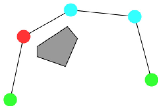
Figure 12.
The key point(red) is determined after adjustment.
Through the SBR algorithm, we can obtain the key point set of the model. Line 20 of Algorithm 1 shows the generation of a smooth path based on the key point set. The steps of smoothing are as follows: according to the key point set and its generating order, these key points are connected by line segments, and then the arc and clothoid are inserted at the position of each turning point (except the key points of the starting point and the ending point). The size of the insertion radius of each part is determined by the constraints and map information. Here, we obtain the optimal radius with the particle swarm algorithm (PSO). The goal is to minimize the cost under the condition of meeting the constraints.
In the PSO algorithm, every particle corresponds to a feasible solution in the optimization domain, and its position and velocity indicate the value and search direction of the solution, respectively. The formula for updating the particle’s position and velocity is as follows:
where and represent the velocity and position of the i th particle in the j dimension at the t iteration, w is inertia weight, and is constant, and are random numbers in the interval [0, 1], is the historical optimal position of particle i, and is the historical optimal position of the group. The PSO algorithm offers notable strengths, including rapid convergence rates and robust global exploration capabilities.
Figure 13 illustrates the position update mechanism in PSO, where the red five-pointed star denotes the global optimum, the blue dots and g represent the individual particle’s historical optimum and the collective optimum, respectively, while the green dots indicate the particle’s current position and its position for the next iteration. Obviously, under the uniform cost condition, the minimum-cost path is the shortest route, and the insertion radius should be the minimum radius.
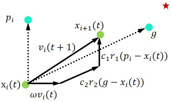
Figure 13.
Pso position update schematic diagram.
The optimization problem (12) involves a large search space due to the joint optimization of multiple constraints. To address this complexity, our two-stage algorithm decomposes the problem into a global coarse search (landmark ordering via Dijkstra) and local refinement (key point adjustment via SBR). This hierarchical approach significantly reduces the search space by decoupling decisions from geometric constraints. Furthermore, the proposed algorithm adopts Dijkstra’s Algorithm to determine the connection sequence of landmark points and conduct point-by-point detection. Dijkstra’s Algorithm itself has deterministic convergence characteristics and can find the shortest path in the graph structure within a shorter time. Although the generation of the point set is based on random sampling, the graph structure constructed through Delaunay triangulation ensures the completeness of spatial coverage, thereby ensuring that a superior solution can be obtained through fewer sampling points within a limited time, and it can also be reflected in the experimental Section 5.2. The time complexity of the SBR Algorithm 2 is , and the time complexity of the entire two-stage Algorithm 1 is .
5. Experiment and Result
This section systematically evaluates the proposed method based on Delaunay triangulation and SBR through comparative experiments designed to verify their effectiveness and superiority.
5.1. Evaluation of Delaunay Triangulation Composition
We first verify the advantages of triangulation over grid. We constructed four map cost functions in total, and the cost range of each map is between 0 and 2, and the map range is . In all maps, the bright yellow part represents the high-cost area, the dark purple part represents the low-cost area, the gray line segments represent the route on the map before smoothing, the black line represents the final path after smoothing, the red point is the starting point, and the blue point is the ending point.
The leftmost sub-image of each image represents the result of the Delaunay method composition, and the number of points is the default parameter; the two sub-images on the right represent the results of the Delaunay and grid methods’ constructions with an equal number of points. The same parameters are used for smoothing, where is set to 0.1 and the maximum curvature is 0.2.
The first function is similar to the non-regular two-dimensional normal function. As shown in Figure 14, the starting and ending points are set at two diagonal positions of the map. It can be clearly seen that although the initial routes of the two compositions are basically the same, the smoothing after composition based on the Delaunay method can effectively avoid high-cost areas, thereby achieving reasonable results. The second function is an elliptical paraboloid, as shown in Figure 15. Unlike the previous one, this time the marginal range of the high-cost area is increased. It can be seen that the smoothing after the composition based on the Delaunay method can still achieve good results, while the grid-based method cannot effectively find the key point. The reason is that based on the composition method of grid, each point has a maximum of four search edges in the horizontal and vertical directions. As a result, on maps with low cost margins and high cost in the middle, the method will strictly walk around the edge of the map, thus marking the key points in advance or delay, which leads to relatively unreasonable results.
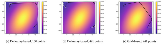
Figure 14.
Compare different composition methods. Map cost function: .
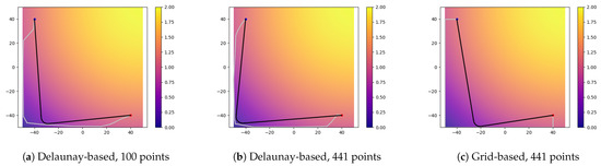
Figure 15.
Compare different composition methods. Map cost function: .
The third function is a plane function, as shown in Figure 16. It can be seen that the grid-based method cannot obtain an ideal result. The reason is that the initial route does not conduct deeper exploration and cannot effectively obtain map information. The cost does not change significantly in each calculation. The fourth function is more like a saddle surface, as shown in Figure 17. It can be seen that the effect of fewer points forming a Delaunay graph structure is similar to the result of the grid method. As the number of points increases, the map information explored will be more comprehensive, and can achieve more ideal results. Table 1 can more clearly display the advantages of composition based on the Delaunay triangulation network.
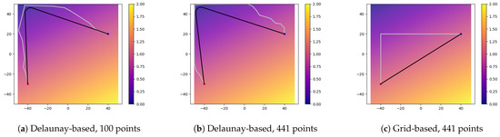
Figure 16.
Compare different composition methods. Map cost function: .
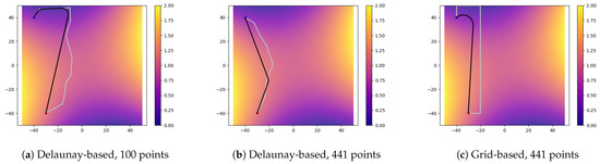
Figure 17.
Compare different composition methods. Map cost function: .

Table 1.
Comparison of effects based on Delaunay and grid.
5.2. Validity and Contrast Experiment
Next, we further verify the effectiveness of the algorithm. Here, we refer to several basic maps in this paper [19] for verification. The environments used for simulation verification include simple environments (Figure 18), concave obstacle environments (Figure 19), cluttered obstacle environments (Figure 20) and maze environments (Figure 21). The size of each map is . The black area in the figure represents obstacles, while the green area, blue area, and yellow area represent areas with 2, 3, and 4 times the cost, respectively. The starting point is red, the ending point is blue, and the landmark point is black. The experimental parameters are as follows: the upper limit of the generating time is s, the generating radius is , the upper limit of the number of generating points is , the maximum curvature is 0.2, the shortest straight line length between the same-direction curves is set to 4, the shortest straight line length between the opposite-direction curves is set to 2, the shortest distance adjustment parameter is 2, is set to 1, the size of the particle swarm is 10, and the maximum number of iterations is set to 20.
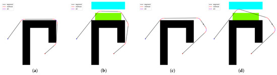
Figure 18.
Solution quality of SBR in the simple obstacle environment. (a) shows the initial situation, (b) adds cost areas, (c) adds landmark points, and (d) shows both cost areas and landmark points.
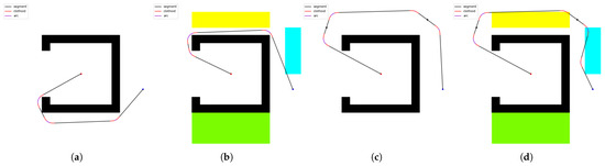
Figure 19.
Solution quality of SBR in the concave obstacle environment. (a) shows the initial situation, (b) adds cost areas, (c) adds landmark points, and (d) shows both cost areas and landmark points.
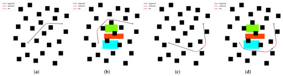
Figure 20.
Solution quality of SBR in the cluttered obstacle environment. (a) shows the initial situation, (b) adds cost areas, (c) adds landmark points, and (d) shows both cost areas and landmark points.
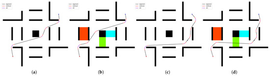
Figure 21.
Solution quality of SBR in the maze obstacle environment. (a) shows the initial situation, (b) adds cost areas, (c) adds landmark points, and (d) shows both cost areas and landmark points.
In these figures, black represents line segments, red represents arc parts, and purple represents clothoid parts. In simple obstacle and concave obstacle environments, when the landmark points and cost areas are not considered, the initial route almost sticks to the obstacles while satisfying the constraints. When both are taken into account, the algorithm has an immediate effect. In relatively complex cluttered obstacle and maze obstacle environments, the comprehensive performance of the algorithm is still reflected. It can be seen that the algorithm avoids or selectively passes through the cost area while completing the target constraints. Taking sub-figure d in Figure 21 as an example, under the premise of passing through the landmark point, the path does not go around the green cost area and walks from below; instead, it selectively passes through to ensure the overall low cost.
We comprehensively compare five well-known methods without regarding to landmark points and cost areas, all using default parameters and the same smoothing method. Because some methods input map information as a graph structure, our time here is counted from the end of the composition. The four map point composition times are 0.12 s, 0.09 s, 1.91 s, and 1.86 s, respectively. The results are shown in Table 2. It can be seen that because the underlying core algorithm is Dijkstra’s Algorithm, our algorithm has a significant advantage in time, and only the JPS algorithm can compete with it. In terms of length indicators, the advantages of the algorithm are also very obvious. Figure 22 is a line chart with a different number of points and path lengths. Our algorithm can achieve excellent results when the number of points is small, converge early, and reduce the running time to a certain extent. It can be seen that on the cluttered obstacle map, the A* algorithm and the JPS algorithm have the same results, while the sampling-based RRT* algorithm and the Informed RRT* algorithm have certain fluctuations.
Table 2.
Comparison of algorithms without regard to landmark points and cost areas.
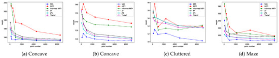
Figure 22.
Line chart with different number of points and path lengths.
Table 3 is a comparison of algorithms considering the landmark points and cost areas. The composition times on the four maps are 0.84, 0.48, 2.41, and 2.76, respectively. When the cost area becomes complex, the composition time will increase significantly. In simple obstacle and concave obstacle environments, the effect of the algorithm is very obvious, and the cost is much lower than other algorithms. On complex maps, the advantage is slight but still obvious.
Table 3.
Comparison of algorithms in regard to landmark points and cost areas.
It is not difficult to understand that grid-based methods (A*, JPS, Theta*) have difficulty meeting multiple constraints in a generating path through grid points, while sampling-based methods (RRT*, Informed RRT*) have difficulty considering the cost of the map. The proposed algorithm constructs the graph through Delaunay triangulation, enabling the map information to be retained with fewer points. It combines the flexibility and exploratory nature of the sampling-based method, as well as the accuracy and efficiency of the grid-based method, so that it can obtain a high-quality solution in a short time.
6. Conclusions and Future Prospects
This paper aims to propose an algorithm to help solve more complex problems or problems not considered by traditional algorithms through mathematical modeling. Through research, we have confirmed the effectiveness of the two-stage algorithm in finding a low-cost path on a map with cost. In addition, the path we find has continuous curvature, avoids obstacles, passes through all given landmark points, and satisfies the minimum length of line segments between curves and the maximum curvature constraints of the curve. We first experimentally confirmed the advantages of composition based on the Delaunay triangulation: it can reasonably and efficiently represent map information. Then, we conducted comparative experiments on four maps. The algorithm can not only generate a smooth path that meets actual needs, but can also maintain good performance while showing strong adaptability to different types of maps and cost functions. In addition, the algorithm’s staged processing method effectively simplifies the problem and provides the possibility for real-time applications.
We believe that there are rich research opportunities in this area. Although our method shows good performance, the following limitations still exist: 1. Under complex maps, the time for key point adjustment will increase significantly, and there may be no solution. 2. The performance of the algorithm depends on the settings of some initial parameters. If the parameters are not properly selected, it may cause the path to deviate from the optimal solution or fail to meet the constraint conditions so that there is no solution. And the selection of some parameters relies on experience and theoretical derivation, which may be good only for themselves instead of being optimal in a global situation. 3. Although using a two-stage algorithm to decouple the problem improves the solution efficiency, it may lose the optimal situation, resulting in path locking in the first stage; that is, the determined connection sequence will limit the adjustment in the next stage. For example, if the suboptimal landmark order is selected when the global path bypasses the high-cost area, the local optimization cannot retrospectively correct this order. Meanwhile, the information fragmentation caused by the separate consideration of cost and constraints leads to insufficient comprehensive optimization ability. The comprehensive consideration of smooth paths may effectively avoid such problems. For example, heuristic algorithms can be used to set key points as variables and constraints as penalty terms for a solution; furthermore, the latest artificial intelligence technology could be used to improve the decision-making ability of the algorithm. Both of these are potential development directions.
In addition, the application prospects across various fields are equally broad. For example, fields such as autonomous vehicles, robot navigation systems, and virtual reality can all benefit from this research.
Author Contributions
Conceptualization, X.D. and L.Y.; methodology, X.D.; software, X.D.; validation, X.D. and L.Y.; formal analysis, X.D.; investigation, X.D. and L.Y.; resources, X.D.; data curation, X.D.; writing—original draft preparation, X.D.; writing—review and editing, X.D.; visualization, X.D.; supervision, X.D. and L.Y.; project administration, X.D. All authors have read and agreed to the published version of the manuscript.
Funding
This research received no external funding.
Data Availability Statement
All data for this study are available from the corresponding author.
Conflicts of Interest
The authors declare no conflicts of interest.
References
- Dijkstra, E.W. A note on two problems in connexion with graphs. In Edsger Wybe Dijkstra: His Life, Work, and Legacy; Morgan & Claypool: San Rafael, CA, USA, 2022; pp. 287–290. [Google Scholar] [CrossRef]
- Hart, P.E.; Nilsson, N.J.; Raphael, B. A formal basis for the heuristic determination of minimum cost paths. IEEE Trans. Syst. Sci. Cybern. 1968, 4, 100–107. [Google Scholar] [CrossRef]
- Sun, X.; Yeoh, W.; Chen, P.A.; Koenig, S. Simple optimization techniques for A*-based search. In Proceedings of the 8th International Conference on Autonomous Agents and Multiagent Systems, Budapest, Hungary, 10–15 May 2009; Volume 2, pp. 931–936. [Google Scholar]
- Harabor, D.; Grastien, A. Online graph pruning for pathfinding on grid maps. Proc. AAAI Conf. Artif. Intell. 2011, 25, 1114–1119. [Google Scholar] [CrossRef]
- Elbanhawi, M.; Simic, M. Sampling-based robot motion planning: A review. IEEE Access 2014, 2, 56–77. [Google Scholar] [CrossRef]
- Karaman, S.; Walter, M.R.; Perez, A.; Frazzoli, E.; Teller, S. Anytime motion planning using the RRT. In Proceedings of the 2011 IEEE International Conference on Robotics and Automation, Shanghai, China, 9–13 May 2011; pp. 1478–1483. [Google Scholar] [CrossRef]
- LaValle, S.M. Rapidly-exploring random trees: A new tool for path planning. Annu. Res. Rep. 1998. Available online: https://msl.cs.illinois.edu/~lavalle/papers/Lav98c.pdf (accessed on 19 May 2025).
- Karaman, S.; Frazzoli, E. Sampling-based algorithms for optimal motion planning. Int. J. Robot. Res. 2011, 30, 846–894. [Google Scholar] [CrossRef]
- Nasir, J.; Islam, F.; Malik, U.; Ayaz, Y.; Hasan, O.; Khan, M.; Muhammad, M.S. RRT*-SMART: A rapid convergence implementation of RRT. Int. J. Adv. Robot. Syst. 2013, 10, 299. [Google Scholar] [CrossRef]
- Faroni, M.; Pedrocchi, N.; Beschi, M. Adaptive hybrid local–global sampling for fast informed sampling-based optimal path planning. Auton. Robot. 2024, 48, 6. [Google Scholar] [CrossRef]
- Huang, T.; Fan, K.; Sun, W. Density gradient-rrt: An improved rapidly exploring random tree algorithm for uav path planning. Expert Syst. Appl. 2024, 252, 124121. [Google Scholar] [CrossRef]
- Miao, C.; Chen, G.; Yan, C.; Wu, Y. Path planning optimization of indoor mobile robot based on adaptive ant colony algorithm. Comput. Ind. Eng. 2021, 156, 107230. [Google Scholar] [CrossRef]
- Cai, Z.; Liu, J.; Xu, L.; Wang, J. Cooperative Path Planning Study of Distributed Multi-Mobile Robots Based on Optimised ACO Algorithm. Robot. Auton. Syst. 2024, 179, 104748. [Google Scholar] [CrossRef]
- Kanayama, Y.J.; Hartman, B.I. Smooth local-path planning for autonomous vehicles1. Int. J. Robot. Res. 1997, 16, 263–284. [Google Scholar] [CrossRef]
- Fei, Z.; Pan, Y.-J. A parameterized cubic bézier spline-based informed rrt* for non-holonomic path planning. In Proceedings of the 2023 IEEE/ASME International Conference on Advanced Intelligent Mechatronics (AIM), Seattle, WA, USA, 28–30 June 2023; pp. 1267–1272. [Google Scholar] [CrossRef]
- Yang, K.; Moon, S.; Yoo, S.; Kang, J.; Doh, N.L.; Kim, H.B.; Joo, S. Spline-based RRT path planner for non-holonomic robots. J. Intell. Robot. Syst. 2014, 73, 763–782. [Google Scholar] [CrossRef]
- Elbanhawi, M.; Simic, M.; Jazar, R. Randomized bidirectional B-spline parameterization motion planning. IEEE Trans. Intell. Transp. Syst. 2015, 17, 406–419. [Google Scholar] [CrossRef]
- Li, C.; Huang, X.; Ding, J.; Song, K.; Lu, S. Global path planning based on a bidirectional alternating search A* algorithm for mobile robots. Comput. Ind. Eng. 2022, 168, 108–123. [Google Scholar] [CrossRef]
- Liao, B.; Hua, Y.; Wan, F.; Zhu, S.; Zong, Y.; Qing, X. Stack-RRT*: A Random Tree Expansion Algorithm for Smooth Path Planning. Int. J. Control. Autom. Syst. 2023, 21, 993–1004. [Google Scholar] [CrossRef]
- Huang, H.C. FPGA-based parallel metaheuristic PSO algorithm and its application to global path planning for autonomous robot navigation. J. Intell. Robot. Syst. 2014, 76, 475–488. [Google Scholar] [CrossRef]
- Bakdi, A.; Hentout, A.; Boutami, H.; Maoudj, A.; Hachour, O.; Bouzouia, B. Optimal path planning and execution for mobile robots using genetic algorithm and adaptive fuzzy-logic control. Robot. Auton. Syst. 2017, 89, 95–109. [Google Scholar] [CrossRef]
- Song, B.; Wang, Z.; Sheng, L. A new genetic algorithm approach to smooth path planning for mobile robots. Assem. Autom. 2016, 36, 138–145. [Google Scholar] [CrossRef]
- Xu, L.; Song, B.; Cao, M. A new approach to optimal smooth path planning of mobile robots with continuous-curvature constraint. Syst. Sci. Control Eng. 2021, 9, 138–149. [Google Scholar] [CrossRef]
- Upadhyay, S.; Ratnoo, A. Continuous-Curvature Path Planning With Obstacle Avoidance Using Four Parameter Logistic Curves. IEEE Robot. Autom. Lett. 2016, 1, 609–616. [Google Scholar] [CrossRef]
- Craus, J.; Polus, A. Aspects of spiral transition curve design. Transp. Res. Rec. 1977, 631, 1–4. [Google Scholar]
Disclaimer/Publisher’s Note: The statements, opinions and data contained in all publications are solely those of the individual author(s) and contributor(s) and not of MDPI and/or the editor(s). MDPI and/or the editor(s) disclaim responsibility for any injury to people or property resulting from any ideas, methods, instructions or products referred to in the content. |
© 2025 by the authors. Licensee MDPI, Basel, Switzerland. This article is an open access article distributed under the terms and conditions of the Creative Commons Attribution (CC BY) license (https://creativecommons.org/licenses/by/4.0/).