Abstract
In the case of a high-risk infectious disease affecting two distinct (without demographic interactions) human populations, e.g., differentiated by their settlement areas, we assume the implementation of a health non-pharmaceutical mitigation policy. However, this policy is based solely on indicators from one of the populations. Using a mathematical model that integrates -SIR representations—where is a variable specific to each population and is governed by a dynamic law (a differential equation coupled to state variables)—the dynamic consequences of the epidemiological processes in both populations are explored and compared analytically and numerically. Mainly, it studies the role of the so-called reaction (intensity of the mitigation) and restitution factor (human compliance).
MSC:
34C60
1. Introduction
From an ecological perspective, two populations of the same species, even if they are indistinguishable in terms of genetics, local adaptation, or growth and reproduction strategies, can still be differentiated primarily by geographical factors, climatic conditions, resource availability, intrapopulation mobility, and ecological interactions. These differences may, to a greater or lesser extent, determine the epidemiological risk associated with a specific pathogen. In the case of human populations, cultural and economic factors further contribute to these variations in risk [1,2,3,4,5].
Indeed, if we consider not only the geographical elements that naturally differentiate two populations, even within the same nationality, but also demographic aspects (e.g., size, structure, and geographical distribution), socioeconomic factors (e.g., education, income, types of employment, housing conditions, or access to goods and services), and cultural factors (e.g., customs, traditions, values, beliefs, practices, or lifestyles), it is likely that the risk associated with the transmission of an infectious disease will vary significantly between populations. All of these variables can play a crucial role, influencing epidemiological dynamics in different ways—either positively or negatively—and can affect the speed and magnitude of contagion, as was observed during the COVID-19 pandemic [6,7,8,9].
The basic reproductive number (), particularly its transmission rate component, commonly referred to as beta, is a crucial epidemiological indicator for assessing the potential spread of infectious diseases within a population. This indicator incorporates various geographic, demographic, and sociocultural factors that influence its magnitude, enabling differentiation between human populations that do not share the same territory. From a geographic standpoint, reflects how environmental characteristics, such as population density and mobility, impact disease transmission. Demographically, this number accounts for population structure, including age distribution, which can affect the average transmissibility of the infectious agent. Socioculturally, is influenced by health practices and behaviors that vary among communities, such as interpersonal distancing and personal healthcare customs. Consequently, basic reproductive numbers or transmission rates can vary qualitatively and quantitatively in their calculation, which can differ from one location to another, thus determining different risk values as an indicator [10,11,12,13].
Without considering individual biological factors, one notable example is the epidemiological differences between urban and rural areas. In urban settings, higher population density may account for variations in transmissibility due to increased interactions and physical proximity. It is well established that economic conditions significantly influence the spread of diseases; thus, in an economically segregated city, the risks of contagion can vary by sector. Cultural practices and levels of education, such as literacy, play a crucial role, as they shape hygiene and preventive beliefs and behaviors that can either facilitate or hinder disease propagation. The geographical environment also serves as a discriminator in transmission dynamics, particularly in relation to climate and the characteristics of the landscape. Furthermore, health systems themselves may differ in terms of resources, intensity, and the quality of preventive or mitigation efforts [14,15,16].
Once a contagious disease is introduced into a territory, health efforts to slow its spread, in the absence of alternatives, typically involve the implementation of non-pharmaceutical mitigation measures, such as restrictions on movement, isolation, mask-wearing, and frequent handwashing. These measures are informed by diagnostic assessments and projections of the epidemiological status of the affected population. However, when the territory is not homogeneous, mitigation measures are not always based on indicators that reflect the situation of the entire area. Instead, decisions may be made for specific subsectors that are more accessible or relevant, even if not in health terms but rather in political, economic, or geographic contexts. For example, in societies with strong centralism, large cities define the health authority’s implementation of ad hoc health management strategies, which may not always be appropriate for the entire territory. This is exemplified by quarantine measures aimed at preventing urban overcrowding, which may not be relevant in rural areas where such conditions do not exist.
In the context of a country, territories can exhibit various forms of fragmentation. Beyond the urban–rural dichotomy mentioned earlier, these territories can also be classified based on geographic factors (objective conditions) or cultural aspects (subjective conditions), including social, economic, ethnic, or religious origins. A mitigation measure perceived as beneficial in one territory may prove detrimental in another. For instance, home quarantines implemented in the same city may seem reasonable overall; however, they can exacerbate overcrowding in social sectors that occupy small residential spaces, such as tenement buildings or cramped houses, which often lack adequate ventilation and increase the risk of contagion. Moreover, territorial fragmentation within a country can extend beyond political–administrative divisions and significantly impact health outcomes. A clear example is found in multinational states, where diversity among national groups can influence pathogen transmission dynamics, leading to variations in the probability of close contact and transmissibility among these groups.
In a fragmented population, where it is distributed across two conceptual or physical patches of a territory, the public health decisions or measures applied to one zone may not reflect its own specific epidemiological reality. Instead, they may be based on assessments from the complementary patch, often the dominant one in this context. When health protocols are imposed from outside, variations may arise in both the intensity of implementation and in the resistance to these measures. Additionally, while the arrival of the disease to the different patches may be diachronic, for simplicity, we will not address that case here. Our focus is on the epidemiological consequences for a temporarily demographically independent subpopulation (e.g., due to the imposition of a preventive lockdown) when a mitigation policy is applied based on epidemiological information from the other patch. For the purposes of this analysis, we will assume that, from the moment the contagion process begins, the patches remain isolated, with no flow of individuals between them.
Methodologically, we will assume two independent subpopulations, each homogeneously distributed within its respective territory, and compartmentalized into the classic susceptible, infected, and recovered groups of the standard SIR model. However, the model will incorporate variable transmission rates for both populations, specifically governed by coupled reaction–restoration dynamic laws of the beta-SIR model, as introduced in [17,18] and complemented in [19,20,21].
In Section 2, from a SIR-type baseline model perspective, we present our model of the evolution of transmission rates for two populations: one of these populations subordinated to the other for the effects of a mitigation intervention based on the epidemiology information of only one of them. The specification of the questions, mainly regarding the impact of the distinction among the behavioral parameters of reaction–restitution, are also found in this section. Section 3 is reserved to show some analytical and numerical answers. This paper closes with a discussion and conclusion, respectively, in Section 4 and Section 5.
2. Materials and Methods
2.1. The Model
Let us consider a human population distributed across a territory , which is divided into two disjoint regions, and . Each region is home to a subpopulation of fixed size, and , respectively. In these areas, we assume that a particular infectious-contagious disease, in the absence of any public health intervention, follows the classic -SIR model. The model operates with constant, intrinsic parameters , where , with the subscript indicating the respective region.
The key assumptions that define the model and contribute to its novelty, particularly regarding dynamic transmission rates, are as follows:
- (a)
- In , based on local information about risk or epidemiological status, a mitigating response is implemented from the outset. This response is also adopted in , but based on the information from . Consequently, in , , a relative reduction in the transmission rate of the form , , is introduced, where represents the reaction coefficient in and reflects the effectiveness of non-pharmaceutical mitigation measures.
- (b)
- Efforts to reduce transmission rates inherently experience strong-type attrition (loss of compliance) or a restoration of the transmission rate, more specifically of exponential order over time. Denoting by the transmission rate at time t in , and letting , the restoration component in , i.e., the instantaneous rate of change in , is given by . The parameter is referred to as the restoration coefficient.
Thus, denoting the state vector of the population resident in by , with , we are considering the differential system:
where
with , gives the SIR character to the dynamics in each subpopulation. Regarding the initial condition for the variables and , these will be taken as and , i.e., their intrinsic values.
In a high-risk epidemiological outbreak without clear alternatives for pharmaceutical palliatives, an authority or a health task force uses indicators to dictate mitigation measures. Immediate examples are the infection rate (e.g., new daily cases per 100,000 inhabitants), the rate of need for hospitalization, or the mortality rate, with the common determinant being the probability that a susceptible person will have contact with an infectious individual. However, aspects such as transmissibility, certain demographic parameters, mobility patterns, or the population’s behavior concerning the same measures may be considered since the control element or criterion may be associated with the potential encounters or contacts that could exist (in ) between susceptible and infectious individuals. In this sense, one possibility is to assume for the reaction factor the form:
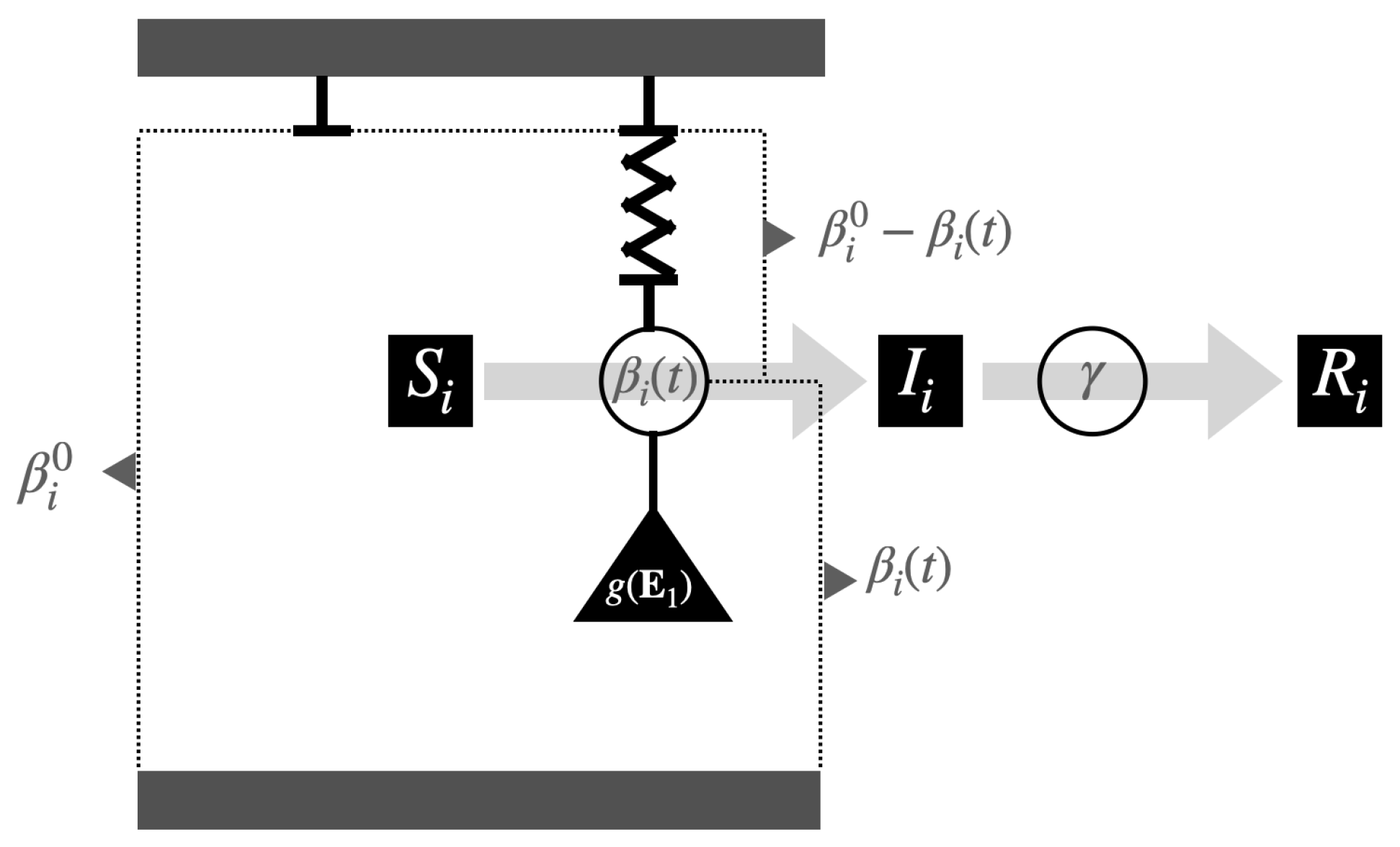
This function assumes a lower intensity at the beginning and end of the epidemic development, that is, when . In addition, note that the factors and , respectively, accompanying in the first two equations of (1) allow us to differentiate and control the strength of the intervention between populations. Table 1 summarizes the model’s variables and parameters, and Figure 1 shows a graphical representation of the (beta, gamma)-SIR model.

Table 1.
Summary of the notation, names, and definitions of the parameters and variables involved in the model.

Figure 1.
Representation of a couple of systems, (beta, gamma)-SIR, in which the transmission rate is influenced by a “force” that seeks to reduce its value (similar to spring extension) and another force that restores the value originating from () through contraction.
2.2. Research Questions
This study focuses on comparing the dynamics of both populations, specifically examining how the transmission rates in () and () are influenced over time. These rates serve as key determinants for the behavior of the other state variables. Consequently, the findings place particular emphasis on these transmission rates.
2.2.1. Comparing According to Intrinsic Rates
The idea is to assume that individuals, when comparing the fragments and , are behaviorally very similar, but that they differ in certain intrinsic conditions. Thus, the assumption is that and , but . In each case (a): and (b): , we will study the epidemiological curves assuming the entry of the disease simultaneously in and .
2.2.2. Comparing According to Reaction Factor
In this case, the idea is to consider , for values of , that is, that is or less or greater than . In other words, to differentiate the intensity with which the mitigation introduced in is replicated in . It is understood that the rest of the parameters are the same, that is, and .
2.2.3. Comparing According to Restitution Factor
In analogy with the previous case, the purpose now is to consider , for values of , that is, that is or less or greater than . In other words, to differentiate the intensity with which the populations manifest their restitution process. It is understood that the rest of the parameters are equal, that is, and .
3. Results
If, from the beginning, the population is connected with the mitigation policy, we see that when in contact with an external infected person with the population:
- (a)
- In , i.e., initial condition , the system reacts according toSo, the transmission rate, in both populations, would go down.
- (b)
- In , i.e., initial condition , the system reacts only by the subsystem, i.e.,Then, without disease in the population, there is no reaction in it, and the population continues with its SIR development following its intrinsic transmission rate.
3.1. Some Analytical Results
We observe that, clearing the term involving from the first two equations of (1), the identity linking the transmission rates of the subpopulations is:
from their integral equations, alternatively
Theorem 1.
Given system (1) and an equilibrium point , then and , with , .
Proof.
In Appendix A. □
So, in the long run infection rates return to the intrinsic rate. That is, the effect that will matter to us, assuming mitigation of another population, is mainly in the early stages of epidemiological development. In what follows, we will denote by , , the fraction that represents the transmission rate of its intrinsic value for the respective population, which will be called relative transmission rate.
Theorem 2.
If in system (1) it has , then , with
In addition, y .
Proof.
In Appendix B. □
Note that to know under what conditions one relative transmission rate is greater or less than another, it is necessary to establish when is greater or less than one. At the moment, we know that and that if the initial conditions for the transmission rates are their intrinsic values, then . Furthermore, since , we have . Regarding the comparison of these relative values in a neighborhood at the beginning of the contagion process, we have the following result.
Theorem 3.
If in system (1) it has , then:
- (i)
- in a neighborhood to the right of , if , i.e., .
- (ii)
- in a neighborhood to the right of , if , i.e., .
Proof.
In Appendix C. □
Let us observe the products , ; they represent some measure of the subpopulation resistance to respect the mitigation in consideration of the intrinsic value of the transmission rate. In this idea, Theorem 3 tells us that a lower (or higher) resistance implies a lower (or higher) relative expression of the rate, as expected a priori.
We can also observe that in terms of , , the first two equations of (1) are such that
This implies that since as , these relative transmission rates evolve toward the value one, similarly to a logistic equation.
An indicator associated with the relative transmission rate is the relative variation in the transmission rate, defined by , .
Theorem 4.
If for system (1) there exists tal que , then , con . Thus,
- (i)
- If , then . In addition, implies .
- (ii)
- If , then . In addition, implies .
Proof.
In Appendix D. □
3.1.1. Comparing According to Intrinsic Rates (, and )
Denoting by and the common values of the restitution and reaction factors, we have the consequences of Theorems 3 and 4. That is, (resp. >) in a neighborhood to the right of , if (resp. >). In addition, considering that , if (resp. ≤), then (resp. ≥).
3.1.2. Comparing According Reaction Factors (, and )
Denoting by and the common values of the factor of restitution and intrinsic rate, respectively, Theorem 4 states that if for system (1) there exists such that , then . Thus,
- (i)
- If , then . In addition, implies .
- (ii)
- If , then . In addition, implies .
3.1.3. Comparing According to Restitution Factors (, and )
Denoting by and the common values of the factor of reaction and intrinsic rate, respectively, Theorem 3 tells us that in a neighborhood of , we have:
- (i)
- If , then .
- (ii)
- If , then .
However, Theorem 4 states that if for system (1) there exists tal que , then . Thus,
- (i)
- If , then . In addition, implies .
- (ii)
- If , then . In addition, implies .
3.2. Simulations and Numerical Results
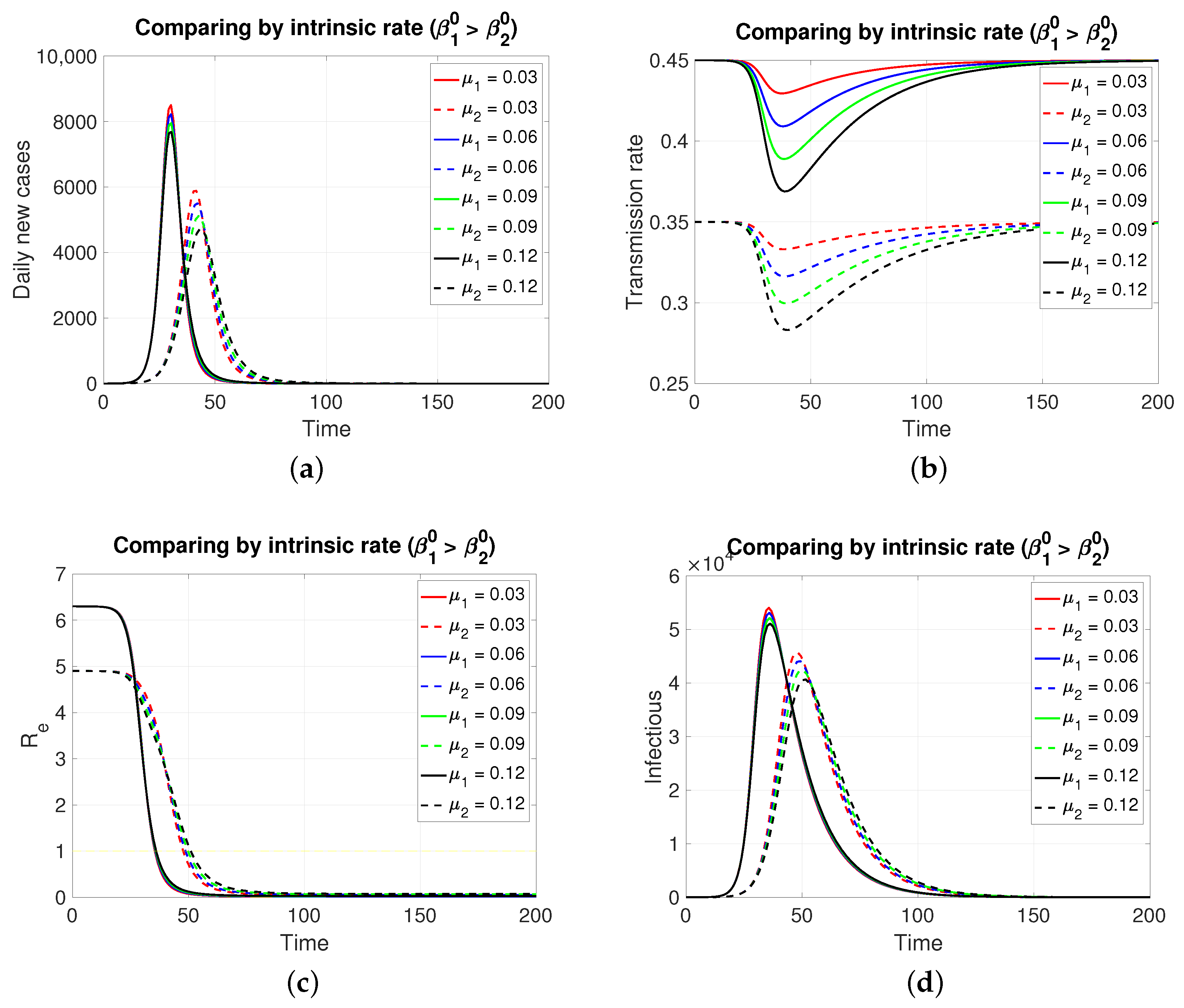
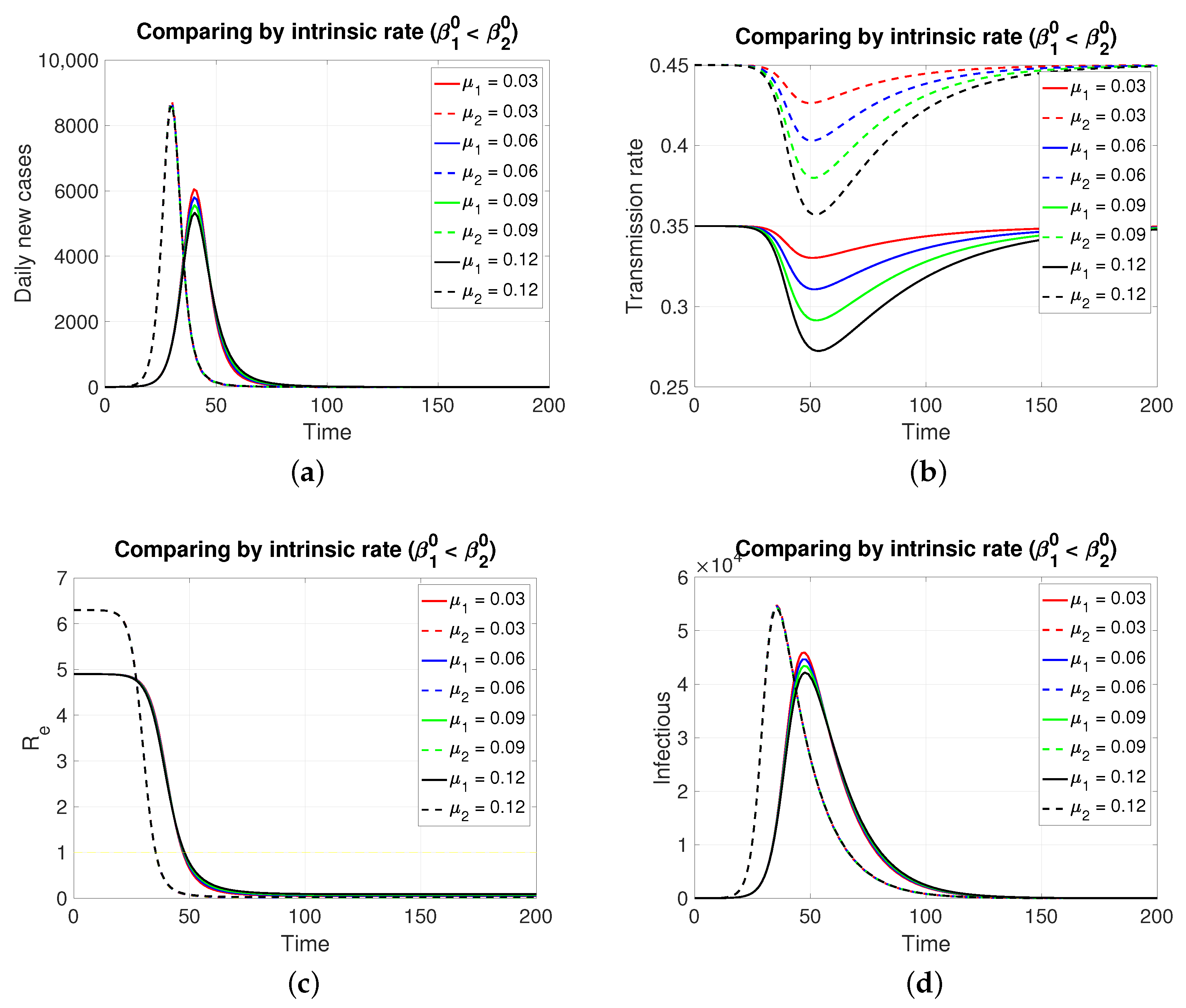
3.2.1. Comparing by Intrinsic Rate (, and )
Since both populations share the same restitution factors () and the same reaction factors (), an increasing series of values for the latter implies a decreasing series of transmission rates for both populations, which is expressed transiently. As expected (Figure 2), the population in , having a lower intrinsic rate than population 1, presents its pulse (segmented lines) of lesser height and later, which is typical of an SIR model. Inversely, if the case is (Figure 3), the population in , having a lower intrinsic rate than population 2, presents its pulse (continuous line) of lesser height and later.
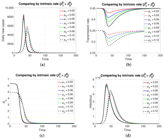
Figure 2.
The figure shows the comparison by intrinsic rate on (a) daily new cases, (b) transmission rate, (c) effective reproductive number, and (d) infectious. Case with , , , , and . This implies . Initial condition: , , 99,999, , and 100,000.
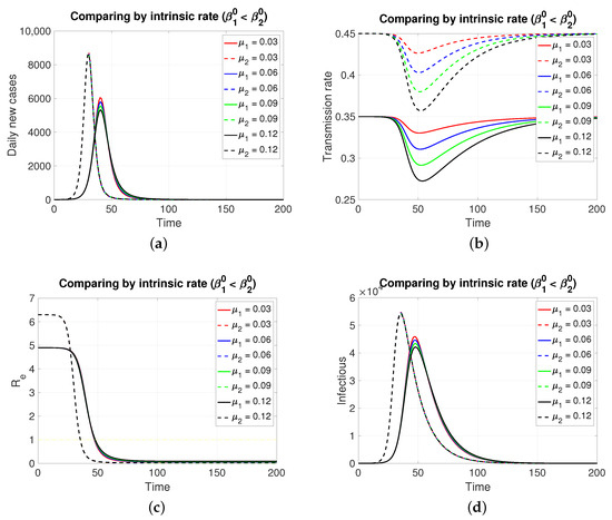
Figure 3.
The figure shows the comparison by intrinsic rate on (a) daily new cases, (b) transmission rate, (c) effective reproductive number, and (d) infectious. Case with , , , , and . This implies . Initial condition: , , 99,999, , and 100,000.
Although, in both cases, the graphs of daily new cases and also the infectious one do not show significant differences for the four values of in , it is clear that in a population of tens of thousands at the peaks of these epidemic curves, the difference in the maximum number of infectious individuals can be counted in units of thousands. Regarding the effective reproductive number, the reduction to zero of its value is faster in the population that presents a higher intrinsic value, i.e., a greater basic reproductive number.
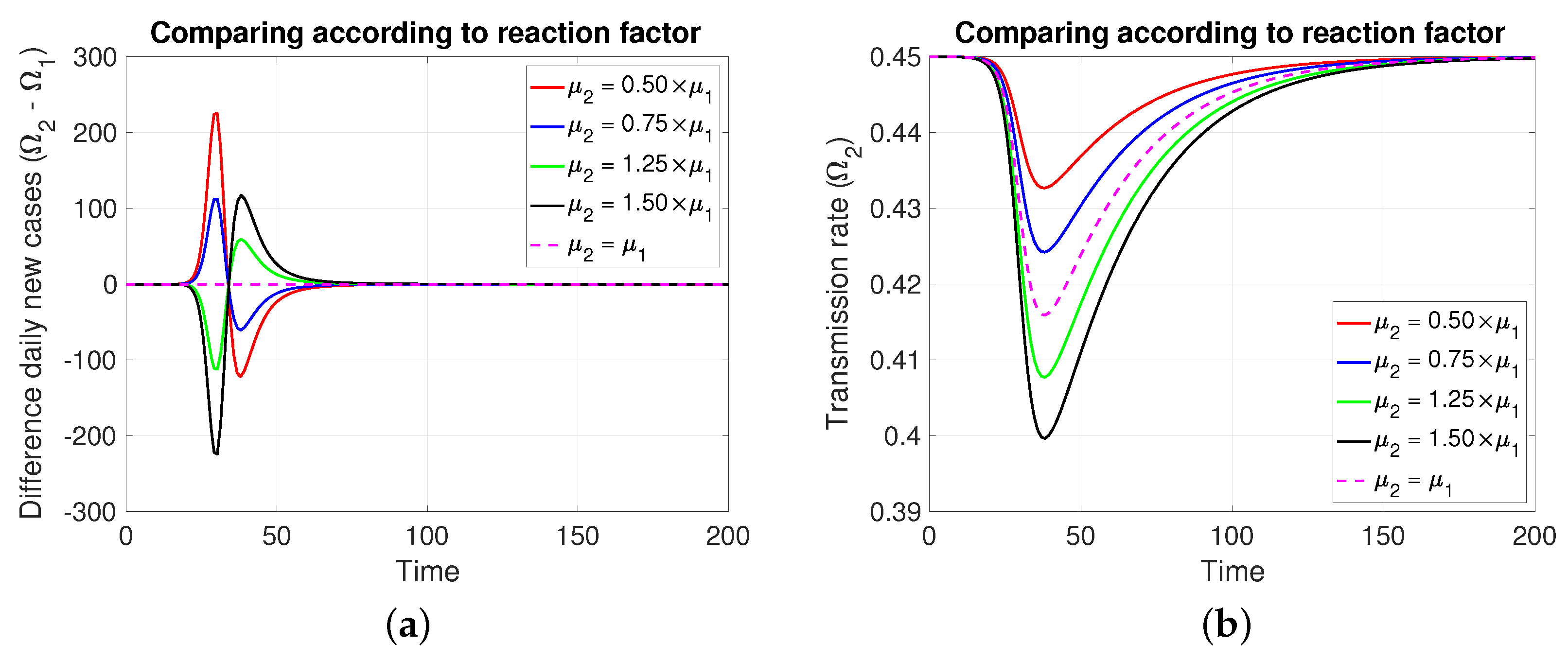
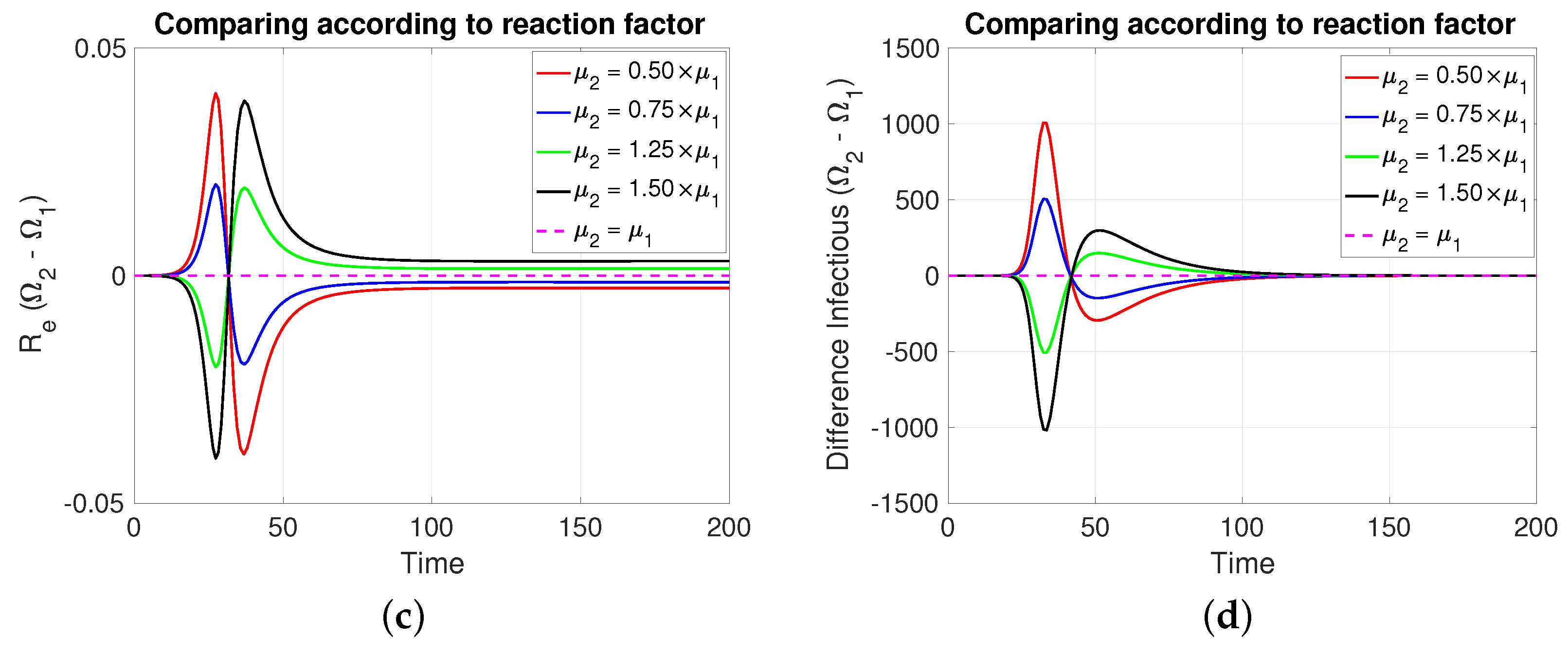
3.2.2. Comparing According to Reaction Factor
Note that in Figure 4, it is assumed, for comparative purposes, that both populations have the same number of individuals and that the contagion process begins at the same instant and with the same initial number of infective individuals. Note that if the mitigation reaction coefficient is higher (resp. lower) in the population of compared to that of , then a greater (resp. lower) number of new cases will be generated in and transiently. However, this is reversed at least after the transmission rate reaches its minimum value.
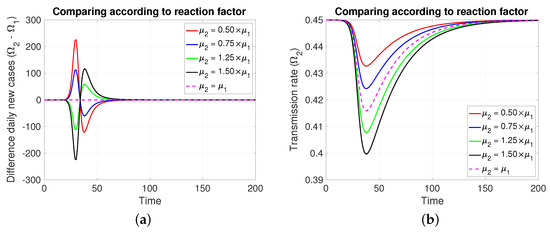
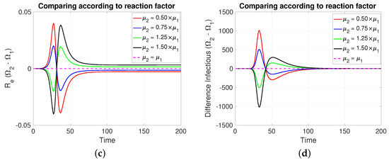
Figure 4.
The figure shows the comparison according to reaction factors on (a) daily new cases, (b) transmission rate, (c) effective reproductive number, and (d) infectious. Case with , , , , and . For the red and blue (resp. green and black) cases (resp. >). Initial condition: , , 99,999, , and 100,000.
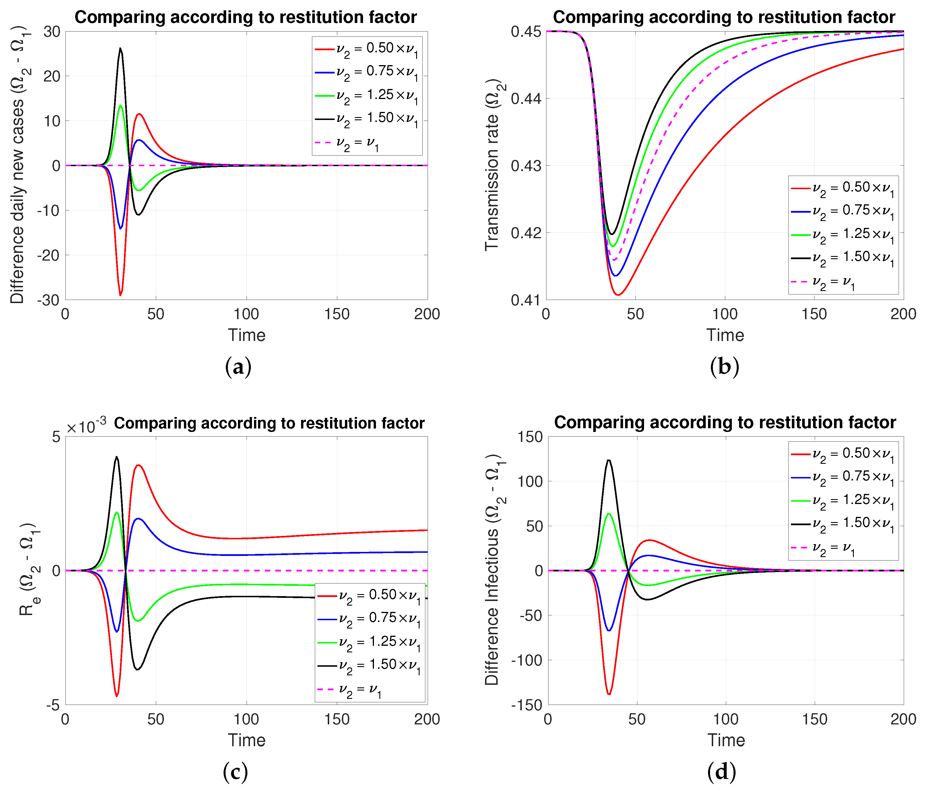
3.2.3. Comparing According to Restitution Factor
In this case, Figure 5 (both in Figure 5a,d, of new cases and active cases, respectively), the dynamic behavior is symmetrical to that of Section 3.2.2 for those about the reaction factor; that is, depending on which coefficient of restitution is greater (resp. less), it produces in a transient way more (resp. less) cases to then invert and subsequently equalize.

Figure 5.
The figure shows the comparison according to restitution factors on (a) daily new cases, (b) transmission rate, (c) effective reproductive number, and (d) infectious. Case with , , , , and . For the red and blue (resp. green and black) cases (resp. <). Initial condition: , , 99,999, , and 100,000.
4. Discussion
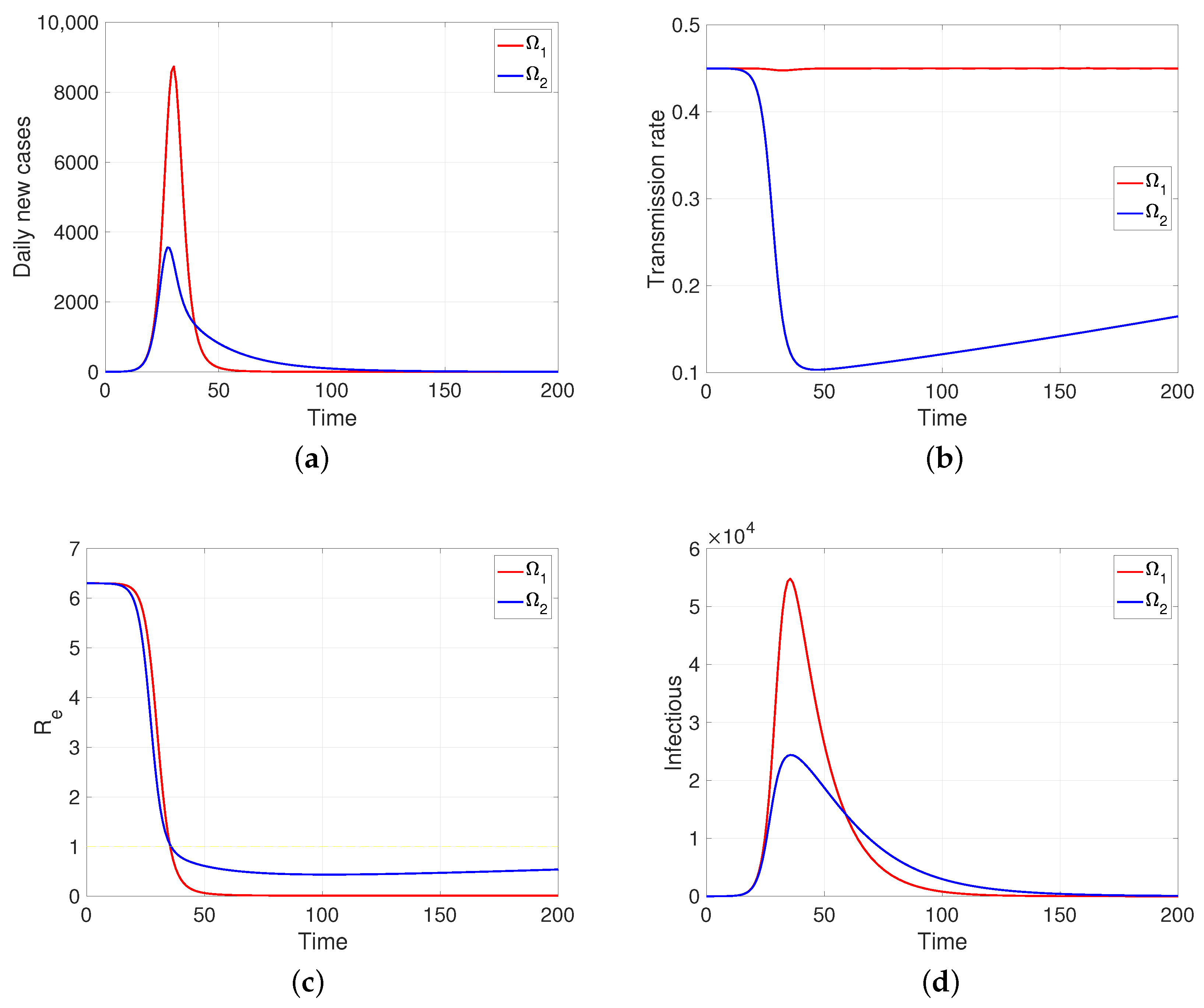
One aspect that the model shows us (as soon as human behavior is introduced into the system, even in the regulated case, i.e., in a specific scheme, in our case the reaction–restoration tension) that the dynamics of the transmission rates can come to mean, for the development of the disease, a great difference between the populations, although they share the rest of the epidemiological parameters. As an example, assuming two behaviorally extreme populations so that comparatively one of them (the one that provides the intervention indicator ) is much less reactive () and at the same time less tolerant to said intervention and the greater tendency to restoration (), the developments of the contagion are those shown in Figure 6, a simulation in which it is assumed that in a pair of populations of one hundred thousand individuals, with the same intrinsic transmission rate and removal time, a first infectious case appears (time zero). It can be observed in Figure 6b that the response to mitigation is much lower in the first population (in red) compared to the subordinate control population (in blue). The difference observed in their effective reproductive numbers is notable; in the index population (red), this indicator is nulled out by the rapid contagion of its entire susceptible population. In summary, subordination mitigation measures, as shown by the simulations, can result in health detriment or benefit for a population, depending on the comparative balance (positive/negative) of key epidemiological parameters, in particular, those we have discussed: intrinsic transmission rates, reaction factors, and restitution factors.
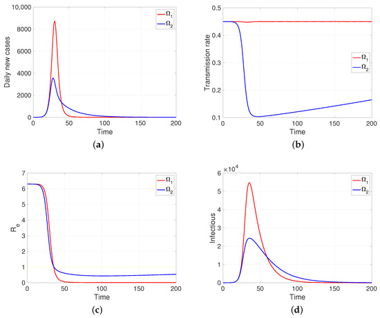
Figure 6.
The figure shows the two behaviorally extreme populations on (a) daily new cases, (b) transmission rate, (c) effective reproductive number, and (d) infectious. Case and . Here, , and . Initial condition: , and . Moreover, 100,000.
For other side, a natural generalization of the model should consider the epidemiological interaction between the populations. This problem, although natural, turns out to be complex if we note that among the determinants of the transmission rates there are not only geographical aspects, which in principle could be assumed to be uniform to the habitats, but also social and cultural aspects that influence them. In general, although concerning proxemics, it is also possible that there may be averaging aspects in the effective encounters between individuals of different subpopulations and the existence of dominance phenomena that may depend on cultural and socioeconomic aspects that are diverse in their expression in space and time. The subject is interesting but outside the scope of this article, so we have planned it for our future research.
It is important to note that the presented model is of a basal order, and therefore, of theoretical value but with low resolution with reality. Now, in terms of advancing in realism, as future work, it is important to mention the importance of demographically connecting the populations and also incorporating the stochastic epidemic models as they are key to avoiding explaining all the noise in the data with the noise of the observation, and, as is known, it is also essential when working with less abundant populations. In this regard, guiding articles related to our topic are [22,23,24], where the latter consider compartmental models and approximate inference. Regarding the connection with the data, we must also consider the tools provided by statistical inference. We highlight the ABC approaches, iterated filtering, or approximate likelihood methods; see, respectively, [24,25,26].
5. Conclusions
The propagation dynamics of an infectious disease varies significantly between populations, even when these populations are under the same non-pharmaceutical mitigation measures; this is due to differences related to sociocultural, economic, and even environmental factors, among others. Therefore, mitigation efforts evaluated as effective in temporarily controlling disease in one population according to local epidemiological indicators, when implemented in another population, will not necessarily have the same control effects.
We know that for the same disease, the intrinsic transmission rate varies according to the population, but at the same time, this rate strongly predetermines the future behavior of the disease in a population. Thus, for the mathematical modeling of epidemiological developments that consider human behavior over time, which alters said rate, either positively (e.g., non-pharmaceutical mitigation) or negatively (e.g., low compliance), it is pertinent to consider a transmission rate through a specific dynamic law. In particular, the law for the coupled relative transmission rates () proposed in this work, for each population, consequently provides us with relevant information that can be considered for decision-making of subordinate population systems from the perspective of the health authority.
The reaction and restoration factors proposed in our model show the impact that a non-pharmaceutical mitigation measure has on daily infectious cases. In particular, the simulations suggest that the spread of the disease is more sensitive to the reaction factor than to the restoration factor. This leads to the conclusion that a non-pharmaceutical mitigation measure focused on raising people’s awareness can be an effective strategy for controlling the disease. However, when applied to another population, this strategy must be evaluated according to the population’s characteristics, that is, measures following the local epidemiological status and its characteristics concerning human behavior.
Author Contributions
Conceptualization, F.C.-L.; methodology, F.C.-L., J.P.G.-J. and K.V.-P.; software, J.P.G.-J.; validation, F.C.-L., J.P.G.-J. and K.V.-P.; formal analysis, F.C.-L.; investigation, F.C.-L., J.P.G.-J., K.V.-P. and R.L.-Y.; resources, F.C.-L. and J.P.G.-J.; data curation, F.C.-L., J.P.G.-J. and K.V.-P.; writing—original draft preparation, F.C.-L., J.P.G.-J. and K.V.-P.; writing—review and editing, F.C.-L., J.P.G.-J. and K.V.-P.; visualization, F.C.-L., J.P.G.-J., K.V.-P. and R.L.-Y.; supervision, F.C.-L.; project administration, F.C.-L. and J.P.G.-J.; funding acquisition, F.C.-L., J.P.G.-J. and K.V.-P. All authors have read and agreed to the published version of the manuscript.
Funding
This research was funded by Agencia Nacional de Investigación y Desarrollo (ANID) through its grant numbers Fondecyt Regular #1231256 and AMSUD220002 MATH-AmSud.
Data Availability Statement
Data are contained within the article.
Acknowledgments
This study was supported by Universidad Católica del Maule.
Conflicts of Interest
The authors declare no conflicts of interest.
Appendix A
Proof Theorem 1.
Suppose that the system (1) is in equilibrium; that is, there exists at least one final value , with , for , which cancels all derivatives. Since , then for , which is expected for a basic SIR model. Since , we must have , that is, , . The above implies that the dynamics are null when the populations do not have infectious individuals. □
Appendix B
Proof Theorem 2.
Note that considering , the first equation of (4) can be written , that is . Finally, . So, amplifying by , we have , an expression that, when integrated in , implies
Now, considering that , we obtain
i.e.,
So, rearranging this expression concludes the theorem. □
Appendix C
Proof Theorem 3.
If we look for a condition to have , according to the previous theorem we need , that is, to ensure that , where
Let us observe that the functions and are such that
In fact, it is enough to note that y and then evaluate at . So, to compare these functions in a neighborhood of , we will proceed by the second-order derivatives. In this regard, we note that:
Therefore,
Thus, to have the condition , it is enough to ask that , that is,
From which, it suffices to ensure that , which corresponds to condition (i) of the theorem. Statement (ii) is obtained by symmetric arguments. □
Appendix D
Proof Theorem 4.
Note that from , , and since , assuming the existence of a time for which , it is concluded that so that
whereby
So, if only if
□
References
- Saker, L.; Lee, K.; Cannito, B.; Gilmore, A.; Campbell-Lendrum, D.H. Globalization and Infectious Diseases: A Review of the Linkages; UNDP/World Bank/WHO Special Programme on Tropical Diseases Research: Geneva, Switzerland, 2004. [Google Scholar]
- Bishwajit, G.; Ide, S.; Ghosh, S. Social determinants of infectious diseases in South Asia. Int. Sch. Res. Not. 2014, 2014, 135243. [Google Scholar]
- Inhorn, M.C.; Brown, P.J. The Anthropology of Infectious Disease; Taylor & Francis: Abingdon, UK, 2013; pp. 31–67. [Google Scholar]
- Farmer, P. Social inequalities and emerging infectious diseases. In Understanding and Applying Medical Anthropology; Routledge: London, UK, 2016; pp. 118–126. [Google Scholar]
- Quinn, S.C.; Kumar, S. Health inequalities and infectious disease epidemics: A challenge for global health security. Biosecur. Bioterrorism Biodefense Strateg. Pract. Sci. 2014, 12, 263–273. [Google Scholar]
- Bharti, N. Linking human behaviors and infectious diseases. Proc. Natl. Acad. Sci. USA 2021, 118, e2101345118. [Google Scholar] [PubMed]
- Funk, S.; Salathé, M.; Jansen, V.A. Modelling the influence of human behaviour on the spread of infectious diseases: A review. J. R. Soc. Interface 2010, 7, 1247–1256. [Google Scholar]
- Sattenspiel, L. Tropical environments, human activities, and the transmission of infectious diseases. Am. J. Phys. Anthropol. Off. Publ. Am. Assoc. Phys. Anthropol. 2000, 113, 3–31. [Google Scholar] [CrossRef]
- Salje, H.; Lessler, J.; Paul, K.K.; Azman, A.S.; Rahman, M.W.; Rahman, M.; Cummings, D.; Gurley, E.S.; Cauchemez, S. How social structures, space, and behaviors shape the spread of infectious diseases using chikungunya as a case study. Proc. Natl. Acad. Sci. USA 2016, 113, 13420–13425. [Google Scholar]
- Sy, K.T.L.; White, L.F.; Nichols, B.E. Population density and basic reproductive number of COVID-19 across United States counties. PLoS ONE 2021, 16, e0249271. [Google Scholar]
- Castro, M.S.M.D.; Tavares, A.B.; Martins, A.L.J.; Silva, G.D.M.D.; Miranda, W.D.D.; Santos, F.P.D.; Paes-Sousa, R. Social isolation relaxation and the effective reproduction number (Rt) of COVID-19 in twelve Brazilian cities. Ciência Saúde Coletiva 2021, 26, 4681–4691. [Google Scholar]
- Salom, I.; Rodic, A.; Milicevic, O.; Zigic, D.; Djordjevic, M.; Djordjevic, M. Effects of demographic and weather parameters on COVID-19 basic reproduction number. Front. Ecol. Evol. 2021, 8, 617841. [Google Scholar] [CrossRef]
- Yu, C.J.; Wang, Z.X.; Xu, Y.; Hu, M.X.; Chen, K.; Qin, G. Assessment of basic reproductive number for COVID-19 at global level: A meta-analysis. Medicine 2021, 100, e25837. [Google Scholar]
- Park, M.; Lim, J.T.; Wang, L.; Cook, A.R.; Dickens, B.L. Urban-rural disparities for COVID-19: Evidence from 10 countries and areas in the Western Pacific. Health Data Sci. 2021, 2021, 9790275. [Google Scholar] [CrossRef] [PubMed]
- Huang, Q.; Jackson, S.; Derakhshan, S.; Lee, L.; Pham, E.; Jackson, A.; Cutter, S.L. Urban-rural differences in COVID-19 exposures and outcomes in the South: A preliminary analysis of South Carolina. PLoS ONE 2021, 16, e0246548. [Google Scholar] [CrossRef]
- Andersen, L.M.; Harden, S.R.; Sugg, M.M.; Runkle, J.D.; Lundquist, T.E. Analyzing the spatial determinants of local COVID-19 transmission in the United States. Sci. Total Environ. 2021, 754, 142396. [Google Scholar] [CrossRef]
- Cabrera, M.; Córdova-Lepe, F.; Gutiérrez-Jara, J.P.; Vogt-Geisse, K. An SIR-type epidemiological model that integrates social distancing as a dynamic law based on point prevalence and socio-behavioral factors. Sci. Rep. 2021, 11, 10170. [Google Scholar] [CrossRef] [PubMed]
- Córdova-Lepe, F.; Vogt-Geisse, K. Adding a reaction-restoration type transmission rate dynamic-law to the basic SEIR COVID-19 model. PLoS ONE 2022, 17, e0269843. [Google Scholar] [CrossRef] [PubMed]
- Córdova-Lepe, F.; Gutiérrez-Jara, J.P. A dynamic reaction-restore-type transmission-rate model for COVID-19. WSEAS Trans. Biol. Biomed. 2024, 21, 118–130. [Google Scholar] [CrossRef]
- Córdova-Lepe, F. On the ways to consider a variable transmission rate in a pandemic strategic SEIR model. In Proceedings of the Communication in Winter School on Mathematical Modelling in Epidemiology and Medicine, Valparaíso, Chile, 19–24 June 2023. [Google Scholar]
- Córdova-Lepe, F. A Newtonian approach to the dynamics of the spread of high-risk infectious diseases. In Proceedings of the Communication in Winter School on Mathematical Modelling in Epidemiology and Medicine, Valparaíso, Chile, 19–24 June 2023. [Google Scholar]
- Lekone, P.E.; Finkenstädt, B.F. Statistical inference in a stochastic epidemic SEIR model with control intervention: Ebola as a case study. Biometrics 2006, 62, 1170–1177. [Google Scholar] [CrossRef]
- Stocks, T.; Britton, T.; Höhle, M. Model selection and parameter estimation for dynamic epidemic models via iterated filtering: Application to rotavirus in Germany. Biostatistics 2020, 21, 400–416. [Google Scholar] [CrossRef]
- Whitehouse, M.; Whiteley, N.; Rimella, L. Consistent and fast inference in compartmental models of epidemics using Poisson Approximate Likelihoods. J. R. Stat. Soc. Ser. Stat. Methodol. 2023, 85, 1173–1203. [Google Scholar] [CrossRef]
- Kypraios, T.; Neal, P.; Prangle, D. A tutorial introduction to Bayesian inference for stochastic epidemic models using Approximate Bayesian Computation. Math. Biosci. 2017, 287, 42–53. [Google Scholar] [CrossRef]
- Ionides, E.L.; Bhadra, A.; Atchadé, Y.; King, A. Iterated filtering. Ann. Stat. 2011, 39, 1776–1802. [Google Scholar]
Disclaimer/Publisher’s Note: The statements, opinions and data contained in all publications are solely those of the individual author(s) and contributor(s) and not of MDPI and/or the editor(s). MDPI and/or the editor(s) disclaim responsibility for any injury to people or property resulting from any ideas, methods, instructions or products referred to in the content. |
© 2025 by the authors. Licensee MDPI, Basel, Switzerland. This article is an open access article distributed under the terms and conditions of the Creative Commons Attribution (CC BY) license (https://creativecommons.org/licenses/by/4.0/).