1. Introduction
In recent years, semantic tools based on word embeddings have become one of the most powerful and widely adopted tools in Natural Language Processing (NLP) [
1]. These embeddings map semantic terms to vectors in high-dimensional spaces, enabling the computation of semantic similarity through distances such as the Euclidean norm or the cosine similarity. The assumption behind these models is that semantic similarity is captured by proximity, that is, in a way whereby two words are semantically related if their vector representations are close in the embedding space.
In this framework, semantic projections have emerged as essential tools for modeling specific features within these semantic environments. Formally, they are functions that quantify how a term expresses a certain property, often modeled as linear functionals over the embedding space [
2]. This allows projecting high-dimensional semantic information onto lower-dimensional features such as size, age, or sentiment [
3]. However, linearity imposes structural constraints that may not align well with the inherent complexity of language, especially when dealing with the non-linear or context-dependent relationships between terms.
The alternative, proposed in [
4], overcomes these limitations by redefining the word embedding process in a fundamentally different mathematical context. Instead of relying solely on linear algebra, this new framework embeds terms into algebras of subsets endowed with a measure and a family of (possibly non-symmetric) metrics. This leads to what is called a set-word embedding, where the semantic representation of a word is given by a measurable subset and its semantic projection is given via a semantic index, which is defined as a proportion of overlap between these sets. This approach yields a more flexible, context-sensitive representation, while remaining mathematically robust through the use of the theory of Lipschitz functions, changing the usual low dimensional linear spaces used in the word embeddings by the more sophisticated Arens–Eells spaces [
3,
4].
In the present work, our aim is to explore two closely related problems concerning the stability of semantic projections across different methodologies. These questions arise naturally in empirical language analysis, where the results of semantic modeling are expected to remain consistent when small changes are introduced into the system. Concretely, two main problems are analyzed. In the first one, stability under different semantic projections are studied. Semantic projections are real-valued functions that measure the intensity of the relationship between two terms, one belonging to a universe of words that describes a given semantic environment, and the other being an external linguistic expression. However, these projections can be defined in different ways, and as a result, their values generally differ even when applied to the same pair of terms. Thus, given a fixed universe of words U and a term t, we analyze how consistent different semantic projections are. In other words, we ask whether the internal “distribution of meaning” through a set of projections is invariant with respect to the index i, thus indicating coherence across multiple interpretative perspectives.
The second one is the stability under changes in the sets of words that we call universes. Given two universes and that are assumed to describe the same semantic environment, we evaluate to what extent the projection vectors and are compatible, in the sense that the overall information that these projection contain is essentially the same. This involves defining methods to compare universes via metrics and estimating how projection values can be transferred or approximated from one universe to another.
Our approach relies on the existence of suitable word embeddings, and it builds upon recent ideas on Natural Language Processing (NLP). The development of distributional semantics has provided a powerful framework for modeling lexical meaning, grounded in the hypothesis that words occurring in similar contexts tend to have similar meanings [
5,
6,
7]. Word embeddings give computational form to this idea by representing terms as vectors in high-dimensional spaces, where spatial proximity captures semantic similarity [
8,
9,
10], and they are widely used across scientific domains to analyze deep relationships among linguistic constructs [
1,
11]. Early models such as Word2Vec [
8] and GloVe [
9] showed that relational and analogical properties can emerge from purely co-occurrence-based representations [
12,
13], paving the way for more sophisticated models of compositionality [
14], contextual variation [
15], and concept-based semantic dimensions via projection techniques [
2]. Note that although this is of primary interest, here, we are not discussing how deep a study based on word embeddings can be or how far-reaching the conclusions might be through their use, despite their well-known limitations [
16,
17]. However, we must at least require that the proposed mathematical methods satisfy some minimal conditions of coherence and compatibility, and this is what we are analyzing here.
Projection-based approaches recover interpretable conceptual features (such as size, gender, or animacy) by aligning word vectors with semantically meaningful axes derived from empirical contrasts. These techniques have been successfully applied in diverse domains, including cross-modal learning [
18], few-shot segmentation [
19], and theoretical linguistics. At a foundational level, this line of research resonates with early insights by Zadeh on fuzzy categories, where linguistic meaning is modeled as graded and context-sensitive rather than crisp and discrete [
20].
In both frameworks that we have considered (vector-valued and set-theoretic) the notion of distance plays a central role. For example, we construct matrices of pairwise distances between elements of two semantic universes and use them to build estimators that transfer projection values across different contexts. These estimators include point-wise approximations (through convex combinations weighted by semantic distance) and global error assessments based on root-mean-square deviation between the estimated and actual projection values.
The theoretical foundation of this methodology is reinforced by formal results showing that, under Lipschitz-type assumptions, the estimation error is bounded and controlled by the projection differences between two terms, t and . This mathematical grounding provides a robust way to evaluate how stable and coherent semantic projections are under shifts in the projection function or the semantic universe.
Thus, the contributions of this paper are threefold. First, we formalize the comparison of projection structures under different and semantic universes, grounding it in both metric geometry, statistical analyses, and AI methods. Following a theoretical background explained in
Section 2, this is done in
Section 3. An example of such an analysis is shown in
Section 3.2, in which we propose computable estimators for semantic projections and their associated correlations, thus offering practical tools for evaluating semantic coherence. A comparison between universes is presented in
Section 4, where a procedure designed by means of the computation on a particular set of terms that are considered relevant is explained. Finally, in
Section 4.4, we illustrate the utility of these tools through a concrete example in the field of agriculture.
Let us recall some basic definitions. If
is a metric space, a function
is said to be Lipschitz if there exists
such that
The infimum constant is denoted by
[
21]. We will work in the examples with the Euclidean norm, but all the results are valid for any distance of a metric space.
Several statistical and AI methods will be used, with the necessary information provided at the point of application.
2. Theoretical Background
The concepts of NLP and the mathematical tools we use in this paper are standard, but some of them come from fields not directly connected to statistics or data analysis, such as Lipschitz continuity. Let us start with a brief summary of the main definitions.
A metric space model is a mathematical structure (in our case, for semantics) that represents semantic terms as elements of a metric space S (the semantic universe), where the distance between these elements represents the semantic distance between the corresponding terms. Recall that a metric is a subadditive and symmetric function such that if and only if . This is the basic assumption in the definition of word embeddings, in which semantic structures are embedded in high-dimensional Euclidean spaces. Thus, semantic similarity between terms (that is, how far two language items are semantically) is measured in the model by the distance
In this context, the notion of set-word embedding is not as well known as the usual linear space-valued word embeddings. Set-word embeddings are also metric models for NLP, but the semantic items are identified with subsets of a fixed set rather than with vectors of a linear space [
4].
As mentioned in the Introduction, a function is Lipschitz continuous if there exists a constant such that the difference in function values between any two points is bounded by that constant times the distance between the points. This condition ensures that the function does not change too quickly, controlling the variation with respect to the metric.
Given a set a class of subsets of S-preserving intersections, we say that a function is a semantic projection (or semantic index as defined below), if it is given as a proportion for another function Broadly speaking, in terms of semantic notions, this definition aims to provide a numerical estimate (a sort of probability) of how a given (semantic) term B shares the meaning of another given term A, normalized by the second term.
In information management, it is usual to consider some similarity functionals on finite sets that are already classical in the setting. The Jaccard (or Tanimoto) index, a similarity measure applied in many areas of Machine Learning, is defined by the expression
for
A and
B finite subsets of a set
where
is the cardinal of the set
The so-called Jaccard distance [
22], which satisfies the requirements for being a metric, is given by
which gives a particular case for a more general version that is the Steinhaus distance for measurable sets
with respect to a positive finite measure
(that is, a countably additive set function,) and it is given by [
23] (§.1.5)
The distance proposed in [
24] is a generalization of these classical metrics, aiming to extend their applicability in broader mathematical and computational settings.
Let us define a semantic index characteristic of the embedding i, based on an asymmetric version of the Jaccard index. In our context, and due to the role it plays in the framework of this work, we refer to it as the semantic index of one meaningful element with respect to another within a given context.
Throughout the rest of this section, we assume that is a finite positive measure defined on a set S, acting over a -algebra of subsets of a set .
Definition 1. Let . The semantic index of B on A is defined asThus, once a measurable set A is fixed, the semantic index becomes a function . Such functions are referred to as semantic projections in [
3,
4,
25]. Informally, this ratio captures the “proportion of meaning” of
A that is explained or shared by the meaning of
B. However, it is important to emphasize that this is a purely mathematical definition. The term “meaning” associated with a set
is simply given by the evaluation of the measure
on
A, where
plays the conventional role of quantifying the size of the set according to a fixed criterion.
In [
25], the notion of semantic projection was introduced to formalize by means of probabilistic indices that represent how a given conceptual item (typically a noun) is represented within a universe of concepts. Thus, given a term
t and a finite universe of words
, the semantic projection
with respect to an element
is a real value contained in the interval
It is defined as a vector of
coordinates in [
25] (§.3.1), where each coordinate is given by
for
,
A natural way of defining a particular case of such a semantic projection is the generalization of a non-symmetric version of the Jacard index defined above. It is based on assigning a set from the
-algebra
to each element of
U and to the term
t. Indeed, let
T be the set considered for all the terms (
) that contains the universe
Then, we define
, and if
is the counting measure, we define
A typical example is the case where
is the family of all subsets of a collection of scientific papers
, and the assignment
associates to each term
t the subset of documents in
that contain it. In the practical applications presented in the following sections, semantic projections are defined precisely in this manner. By considering the counting measure
over the
-algebra of subsets of a given document repository, we compute the ratio between the number of documents in which both terms
t and
co-occur and the number of documents in which
t appears.
To summarize the conceptual structure introduced in this section, we outline below the essential components that define our analytical framework.
A lexical domain, that is, a finite set of linguistic items, such as words, short expressions, or terms, denoted by W, which serves as the base vocabulary for constructing a contextual semantic model.
A measurable semantic space, which is a finite measure space , where is a sigma algebra of subsets of , and each element of W is associated with a measurable subset in . In this paper, will be finite, the class of all subsets, and the counting measure.
An embedding function, which is an injective mapping that assigns to each term in W a unique measurable subset of . This mapping is well defined due to the assumption that all images lie within the -algebra .
A word embedding , which allows us to identify each term with a vector of a finite dimensional real linear space.
3. Coherence Analysis of Semantic Projections: Statistical Approach
As we said, in the rest of the paper, we work with a finite set and the class of all its subsets as the measurable space
and the counting measure as
Consider the vector that defines the semantic projection on a term
t on a universe
of semantic items. That is, given a concrete semantic projection (formally, a measure on a finite set as defined in
Section 2 in (
1)), we fix the vector
that represents the term
t in
U with respect to the projection
We follow the notation introduced in the last section. It is supposed that we have different projections
and the objective of this section is to assess how far all of them give similar information, that is, how far all together confirm the information on the “real value” of the sharing degree contained in each of the coordinates of such vector. Consequently, we use some statistical concepts to analyze this question.
Thus, we have to deal with a finite set of semantic projections of a term t into a given universe In the applications of the model, each projection is provided by a search engine, such as Google, or a database of scientific documents, such as DOAJ. The order of the terms of U is fixed.
If
T is the set of all terms, we have to consider several functions
where
denotes each of the semantic projections taken into account.
Therefore, once a universe is fixed, each term t and each projection produce a vector with coordinates between 0 and
In this section, we consider the normalized vectors associated with a fixed term t. The motivation behind this normalization is to evaluate whether the relative weights of the coordinates of each projection vector are independent of the index . That is, we are interested in studying the internal distribution of information within each vector, regardless of its magnitude.
3.1. Analytic Procedure
Given a fixed term
t, we define the normalized projection vectors as follows:
where
denotes the standard Euclidean norm in
. To interpret the structure and similarity of these normalized vectors, our method involves the computation and visualization of the following items.
- (1)
Correlation analysis.
We compute the
correlation matrix of the vectors as follows:
where
denotes the standard inner product in
. This matrix quantifies the angular similarity between the normalized projections. We represent this matrix visually using a heatmap. Our aim is to provide a clear measure of how different the vectors are when representing various sources used to compute the semantic projections. Since correlation analysis is a standard procedure in experimental science and data analysis, it offers clear and direct information to potential users of our method.
Additionally, we have computed a chi-square similarity matrix based on the coordinate-wise comparison of and , and we also visualize it via a heatmap. This alternative emphasizes component-wise differences when interpreting the normalized weights as probability distributions. This approach provides a visual tool to represent the proximity between different sources of semantic projections, offering an even more straightforward understanding than correlation analysis.
- (2)
Clustering of semantic profiles.
We treat the normalized vectors as points in , and we apply clustering algorithms to explore grouping patterns. In particular, we perform the following:
- –
Apply Principal Component Analysis (PCA) to project the data into two dimensions for visualization.
- –
Perform k-means clustering for , showing the resulting clusters with graphical representations in the PCA plane.
- –
Use the Elbow method to determine the optimal number of clusters.
With the use of these procedures, we intend to improve the selection of which semantic projection methods can be considered equivalent as well as appropriate. The main cluster is used to discard the sources that are not providing adequate responses from the interpretational point of view.
- (3)
Representative or average result.
For applications, and following the identification of clusters or highly correlated groups of vectors, we can compute the mean of the original (non-normalized) vectors
within the main cluster or those with high correlation to a selected reference vector. This average could serve as a representative projection pattern for the term
t.
where
is the set of indices corresponding to the selected cluster or correlated group.
This provides a full and comprehensive description of the properties of the semantic projections, allowing us to assess whether the results are coherent (in the sense that they follow similar trends), and if so, to compute a meaningful average value that synthesizes the overall outcome. Note that the groupings proposed depend on a fixed term.
3.2. A Case Study on Agricultural Terms Using Four Semantic Projections
Let us show an example of our methodology. We consider the universe , and the term “plowing” to compute the semantic projections onto U.
3.2.1. Data Collection and Sources
We focus the attention on the following four different search engines: DOAJ [
26], Google Scholar [
27], Google [
28], and Arxiv [
29]. The normalized results obtained for each source are shown in
Table 1.
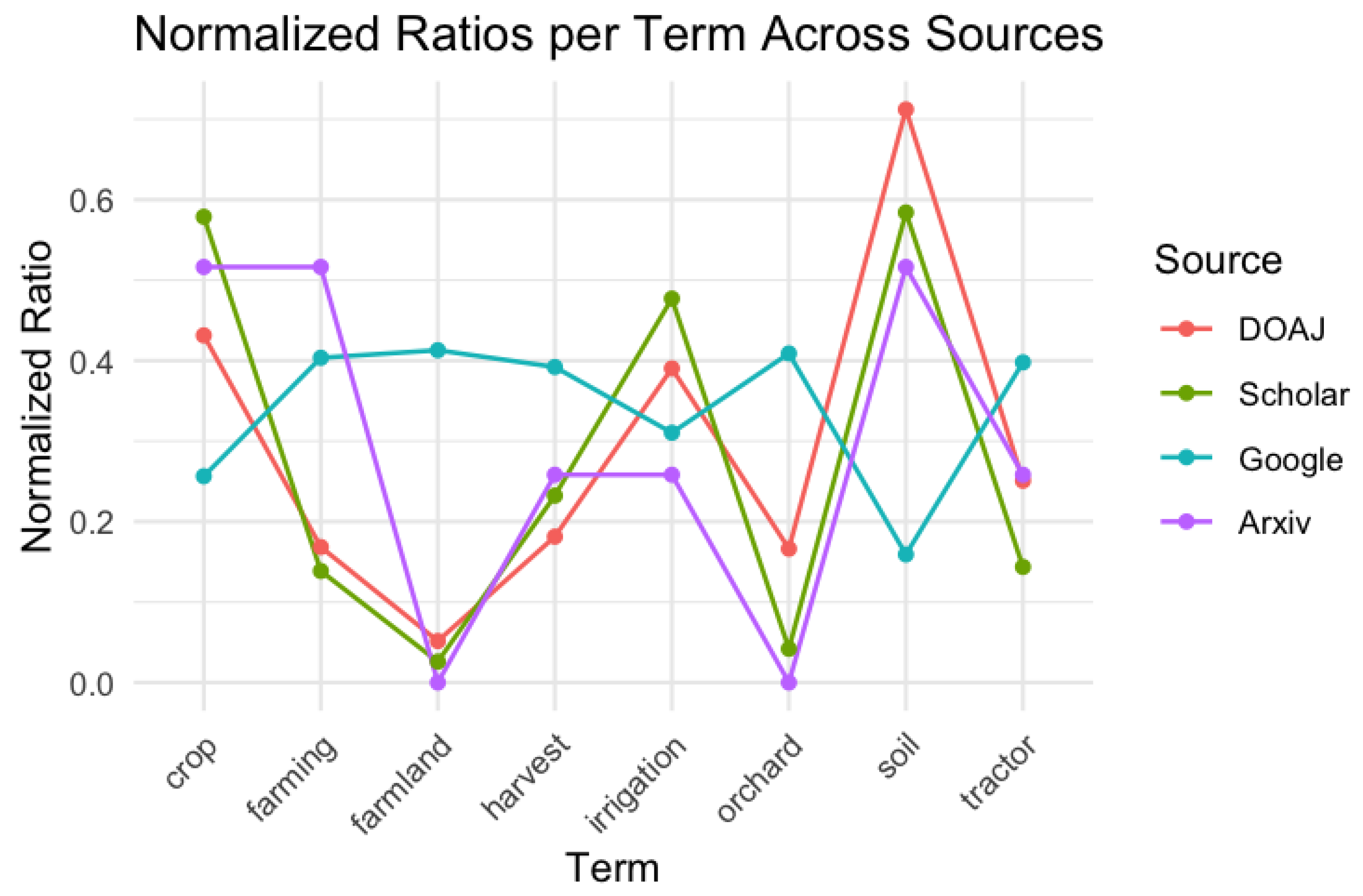
As can be seen, terms such as “soil” and “crop” are most associated with “plowing” across all platforms, although the importance varies by source. Google tends to distribute semantic weight more evenly, while DOAJ and Scholar show a greater emphasis on a few agricultural terms, indicating a more focused context.
3.2.2. Semantic Projection
The raw data obtained in the previous step are now graphically analyzed using explicitly the concept of semantic projection. The results can be seen in
Figure 1. The representation of the curves gives visual proof that DOAJ, Scholar, and Arxiv follow the same trends, while Google shows a different picture.
3.2.3. Statistical and AI Methods
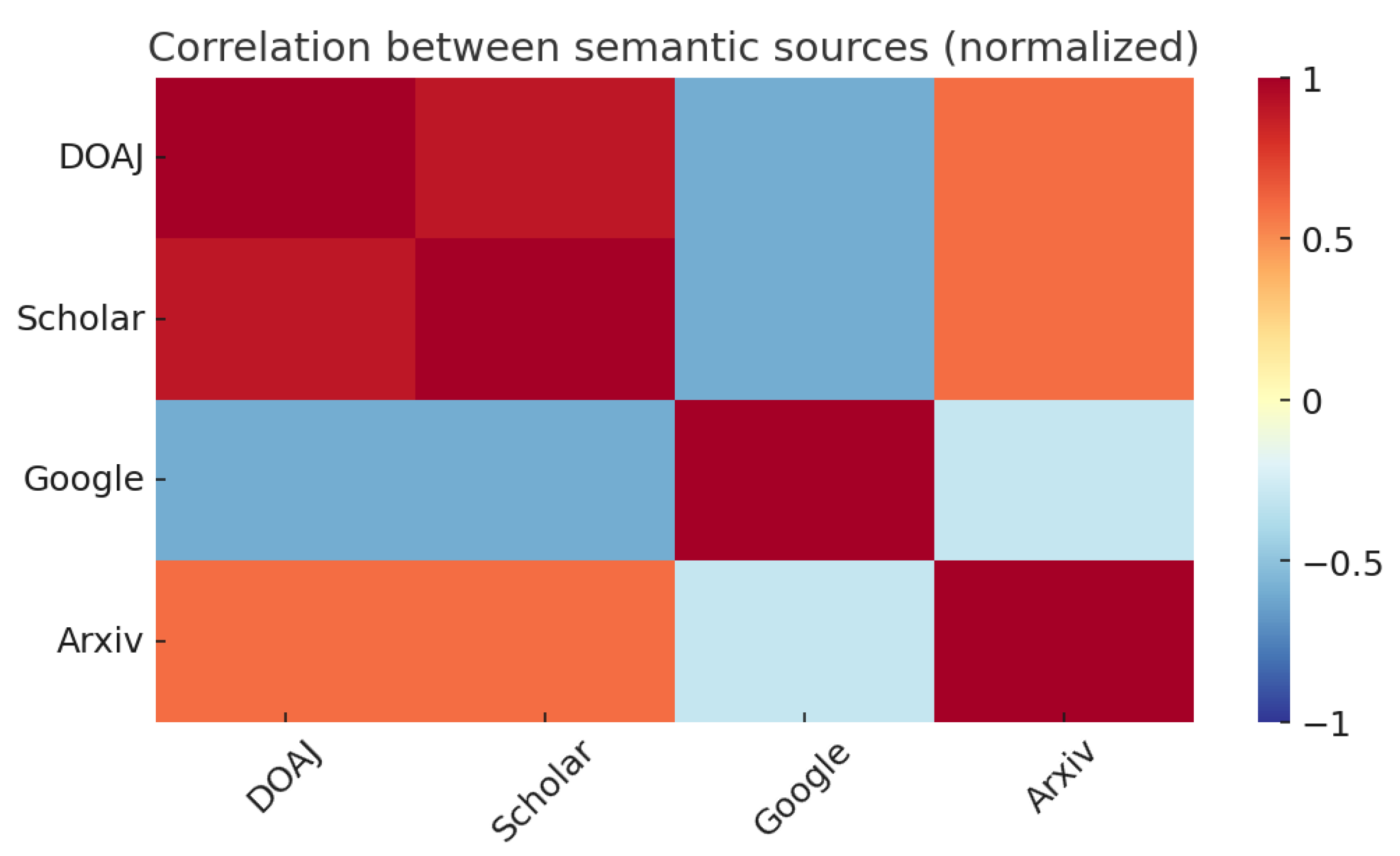
The relations between these semantic sources are presented in the correlation matrix shown in
Table 2. As expected, DOAJ and Scholar show a very high positive correlation (
), suggesting that both repositories contain articles with agricultural contents in a very similar way. Arxiv also shows a positive correlation, although somewhat weaker, with these sources, probably due to the low representation of articles present in this collection. In contrast, Google exhibits strong negative correlations with DOAJ and Scholar, highlighting how it behaves differently.
This behavior is explained graphically in
Figure 2, where a heatmap of the correlations is shown. While the other searches are conducted within a “closed” set of scientific documents, such as peer-reviewed articles or curated repositories, Google indexes a much wider range of sources. As a result, it may lead to connections that are not necessarily meaningful or directly related to the actual co-occurrence of the specific terms being investigated.
A chi-squared distance heatmap (
Figure 3) also provides complementary information. As can be seen, smaller distances in blue confirm the closeness between DOAJ and Scholar, while Google appears more distant from the academic repositories.
A Principal Component Analysis is also developed. The results summarized in
Table 3 reveal that more than
of the variance is captured by the first principal component. This indicates that the main semantic variation between sources can be mostly explained by a single underlying factor.
Next, and confirming the previous results,
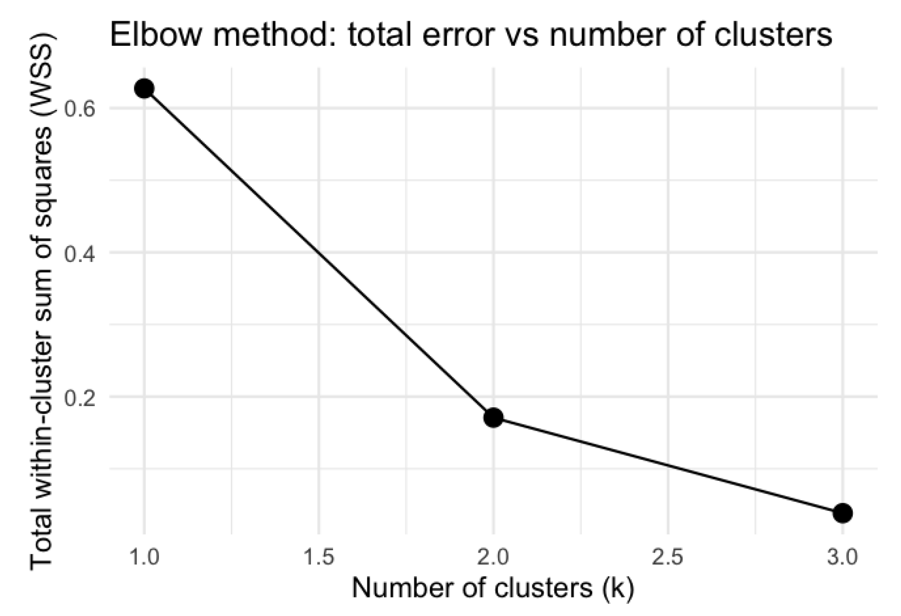
Figure 4 presents the optimal clustering into two groups (the first one containing three elements; the second, one element), clearly separating Google from the academic sources.
Figure 5 provides a representation of the total within-cluster variance as a function of the number of clusters. The“elbow” at
confirms that two clusters are the most natural choice for this dataset.
The effectiveness of the method depends on whether the volume of data is large enough to ensure a certain statistical stability. In very specific contexts, the procedure we propose could easily fail, depending on whether the relevant terms share a sufficiently large set of documents to make the corresponding ratios non-trivial or avoid a strong sensitivity to small variations in term frequency.
3.2.4. Evaluation Metrics and Analysis Procedures
Let us sum up, in what follows, the results of the application of our analytical procedure. All the information provided in the previous steps can now be integrated to offer a global view of the results. Thus, in general, Scholar, DOAJ, and Arxiv show a strong consistency in their treatment of agricultural and water-related vocabulary, while Google presents a significantly different semantic pattern. This divergence is expected, since Google indexes a big amount of documents, from highly specialized scientific papers to more informal or journalistic content. Therefore, although some agricultural terms are present, their semantic connections to specialized activities such as “plowing” become less consistent. In contrast, sources like DOAJ, Scholar, and Arxiv are restricted to academic and technical articles, where vocabulary tends to be more focused and contextually coherent. This explains why, across the semantic projections, Google exhibits negative correlations with Scholar and DOAJ (around
), as shown in
Table 2 and
Figure 2. The chi-squared distance heatmap in
Figure 3 confirms this fact.
These results suggest an important methodological point as follows: when analyzing specific technical contexts using semantic projections, the choice of repositories or search engines strongly influence the resulting structure. This fact has to be taken into account for the relational analyses based on multi-source semantic projections.
Finally, the average result can be computed as just the average value of the vectors defined by DOAJ, Google Scholar, and Arxiv. This could be useful when a unified result is needed for further analysis.
4. Comparison of Universes: Semantic Stability in Metric-Based Models
In this section, we consider two universes of terms, and , containing and elements, respectively. Our goal is to introduce and analyze different methods for comparing these universes. The underlying assumption is that both aim to describe the same semantic environment, and we seek to determine whether they actually do so. To this end, we propose comparing the semantic projections of certain reference terms within each universe. These comparisons serve as the basis for assessing whether both universes effectively represent the same semantic content.
The comparison method we propose follows a similarity-based approach, organized through the following steps.
- (1)
Fix a finite set A of testing terms, and select a concrete semantic projection P defined on a set X that contains both and
- (2)
Compute the semantic projections of all elements onto both universes and .
- (3)
Using one of the methods proposed in the following sections, compute estimates of the semantic projections based on and the similarity between the elements of and , where similarity is measured by the distance d between embedded vectors.
- (4)
Compare the direct values of the semantic projections with their corresponding estimates for all .
- (5)
Evaluate the performance by calculating the quadratic error between the actual and estimated values of the projections.
The methods proposed for this comparison are discussed in separate subsections. In both approaches, the elements of and are embedded into a metric space via a word embedding . This allows the use of standard distance metrics in , such as the Euclidean norm, to compute similarities or differences between the universes. It is important to note that we do not assume and contain the same number of elements.
Fix a word embedding I into such that all terms in both universes and can be embedded. Instead of relying on the Euclidean norm, we consider a general metric d defined on , which allows for a more flexible notion of distance between elements in the semantic space.
The metric model is then based on the matrix of pairwise distances between embedded terms from each universe
Using this matrix, we define a proximity function
D between the two universes as the sum of all the pairwise distances
This function is symmetric, but it is not a true distance, since
only in trivial cases. However, when the context is fixed, it can serve as a meaningful measure of how far apart the universes
and
are in semantic terms.
In addition to this metric-based estimate of proximity, we are also interested in estimating the semantic projection of a given term t at each concept , using only the known values of for .
To do this, we define for a fixed term t as a weighted average (convex combination) of the values , where the weights are calculated in terms of the distance between and each in the embedding space. We propose three procedures.
Remark 1. Notice that we propose a metric model. Accordingly, we expect that the semantic projections, as described in other works, preserve the distance-related parameters. Thus, semantic projections, regarded as real-valued functions, are assumed to preserve the distances in the metric space where they are defined. The natural requirement in this direction is that they are Lipschitz functions with controlled Lipschitz constants.
4.1. Uniform Distribution of the Weights in the Extension
First, for each fixed
, define the normalization factor
Then, the estimated projection
is given by
This expression yields a convex combination where each weight increases as the distance
decreases, assigning greater influence to the semantically closer elements. As we will see later, other weight values with the same property can be implemented to yield alternative estimations.
The error committed when approximating
by
is measured by the following:
This gives a point-wise error for each term
t. By averaging this error over a sufficiently large and representative set of terms, we obtain a global estimate of the stability of the projection across the universes. A small value of this quantity suggests that the
and
are semantically compatible and yield consistent projection behavior. Under the assumption that the projection function
is Lipschitz continuous with respect to the metric
d, it is possible to derive a theoretical upper bound for the error
, further supporting the validity of the approximation.
Let us now establish the result concerning the Lipschitz-type properties of the proposed model. We assume the existence of a word embedding that allows us to compute the values of . However, there are no restrictions on how the metric d is defined. In standard settings, d is typically the Euclidean distance. It is worth noting, however, that the cosine distance (although frequently used) cannot be applied in this context, as it does not satisfy the axioms of a true metric.
Theorem 1 (Lipschitz continuity of the projection estimator)
. Let t and be two terms, and let and be two semantic universes. Assume that the semantic projections are Lipschitz continuous in t with constant , that is,Then, for each , the estimated projection satisfiesIn particular, the estimator is Lipschitz continuous with respect to the term t, and its Lipschitz constant is bounded above by L. Proof.
Fix
and consider the difference
The weights
defined as before are given by
where
are the normalization factors defined in (
2). We
claim that the addition of all these weights with a fixed
j equals
Indeed,
which is equal to
by the definition of
. □
Note that this approach does not define an extension of the original function. That is, if we put as search term an element of the original universe , the solution is not necessarily the projection on this element. Furthermore, as will be shown in the final example of the paper, this extension tends to assign an average value to all estimates, making it difficult to clearly distinguish between the semantic projections of different elements of the universe. To address these issues, in the next section, we propose a different method for defining the weights, modifying them so that the elements of the universe closer to the target vector receive stronger weighting.
4.2. Hierarchical Weight Distribution
This approximation is computed separately for every element
So let us fix and index
j (that is, an element
), which will be considered to be fixed throughout the following steps. Here, the distance
d is the one provided by the Euclidean norm. Consider the map
given by
and the associated inverse ordering given by
, if and only if
(note that, for the sake of simplicity, we do not explicitly refer to the index
j in the notation of
).
We define the weights of the convex combination according to the next tool. Reorder the set
using the ordering
and reindex
increasingly with respect to this ordering as
Thus, we define the weights as follows. Let us write
for
and following in this fashion until the last index, which will be different, given by
Let us show that the sum of these weights is in fact equal to
Theorem 2. Fix a point . Let be a metric space, and let be a finite set. Definewhere I is a given embedding into the metric space Order the elements increasingly, according to (i.e., the closest first), and normalize the distances by setting Define recursively the weights asfor , and for , Then, and the approximation formula obtained with these weights is an extension of the function given by
Proof.
The proof is the result of a direct computation. Note that the required addition gives
If we group the terms recursively, each product accounts for the proportion of the unity not yet assigned, and the last term collects the remaining part. Note that this expression is a telescoping-type expansion
, which always sums to 1. Thus, the total sum of the weights equals 1. □
As in the other cases analyzed before, it can be easily seen that this approximation preserves the Lipschitz constant of the projection
, following the same arguments as in the proof of Theorem 1. Finally, note that the estimated projection will be in this case represented by
This expression yields a convex combination where each weight increases as the distance
decreases, assigning greater influence to the semantically closer elements.
4.3. Lipschitz Extensions and Regression Estimation
The classical formulas of McShane and Whitney for extending Lipschitz functions can also be used to obtain estimates of suitable extensions of the projections, in the context of what is called Lipschitz regression (see, e.g., [
25,
30,
31] and the references therein). The advantage of this technique of regression is that, as in the previous cases, only a metric is required on the space, without restrictions involving the use of linear structures.
Real Lipschitz functions on any metric subspace of a metric space can always be extended to the whole space with the same Lipschitz constant. Suppose that we have a function f defined on a subset and we aim to extend it to all of X while preserving .
Although there are many possible extensions, there are two classical formulas that have also the advantage of being the minimal/maximal extensions preserving
. That is, any Lipschitz extension
F preserving the constant satisfies
Those formulas are the minimal (sometimes called the McShane) extension,
and the maximal (Whitney) extension,
Moreover, for any
,
is a valid Lipschitz extension with constant
L. The usual election for the interpolation parameter is
As with the previously explained techniques, we can use McShane–Whitney formulas to predict the unknown projections
based on the known values
. Basically, the method follows the same steps that the previous ones did. First, we compute the distances
for all
i, and for each
, we calculate
as well as
Then, we estimate the projection by
or adapting the value of
if needed.
Remark 2. Note that the average value (3) always belongs to the interval , sinceIndeed, we know that Note also that the Lipschitz constant
L has to be previously estimated as the following maximum ratio between differences of known projections and their distances,
In this case, by definition and by taking into account the nature of the McShane and Whitney formulas, the proposed method is an extension of the projection defined as acting in Note that these formulas are not restricted to values in when , so this condition must be enforced if needed.
4.4. Universe Similarity Analysis: A Case Study
In this section, we conclude the explanation of the comparison method we propose, based on a set of single-term estimates of a chosen semantic projection. An agricultural context is also considered in this example. The analysis that follows proceeds through the following steps.
- (1)
First, we fix two universes and , which are assumed to describe similar semantic contexts, and a semantic projection to measure its stability under the change from to .
- (2)
Fix a finite set of terms S for comparison. For each , compute the values of the semantic projection and , where and .
- (3)
Use the methods explained in the previous section to obtain an estimate of the value of for every and .
- (4)
Compare the estimates with the true values by measuring the quadratic error between them.
We will now explain the procedure through a concrete example. Let us explain the details of the example in the following. Note that the words have been chosen to describe a semantic context.
4.4.1. Data Collection and Sources
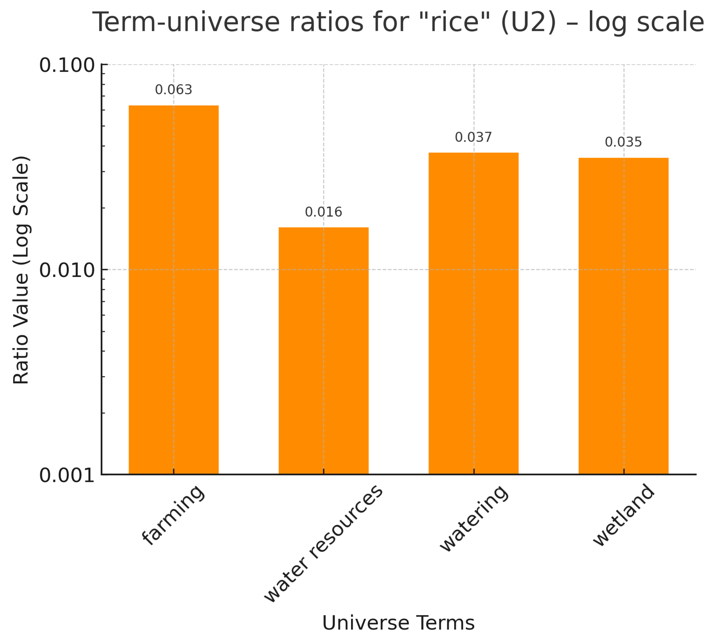
We choose a simplified semantic environment related to water resources and agriculture, and the universes
which we consider to be similar for describing this semantic context. We consider just one term for comparison in the set
which is assumed to make sense in the corresponding environment. We choose the term
t = “rice”. The distances matrix shown in
Table 4 has been computed using GloVe (small size version GloVe 6B 50d [
32]).
4.4.2. Semantic Projection Techniques
We fix the semantic projection defined by the computation of the joint occurrences of two terms within the documents retrieved through the DOAJ (Directory of Open Access Journals) search engine. The results of all projections are written in
Table 5 and
Table 6.
4.4.3. Statistical and AI Methods
Next, we compute all the estimates of the values of
following the three methods explained in the previous section, in order to compare with the real values calculated using the direct semantic projection computation. Here, for the sake of clarity, we call them the Averaged Weights Method (Averaged W.), Closer Weights Method (Closer W.), and McShane–Whitney Method (Mc-W). The results are given in
Table 7.
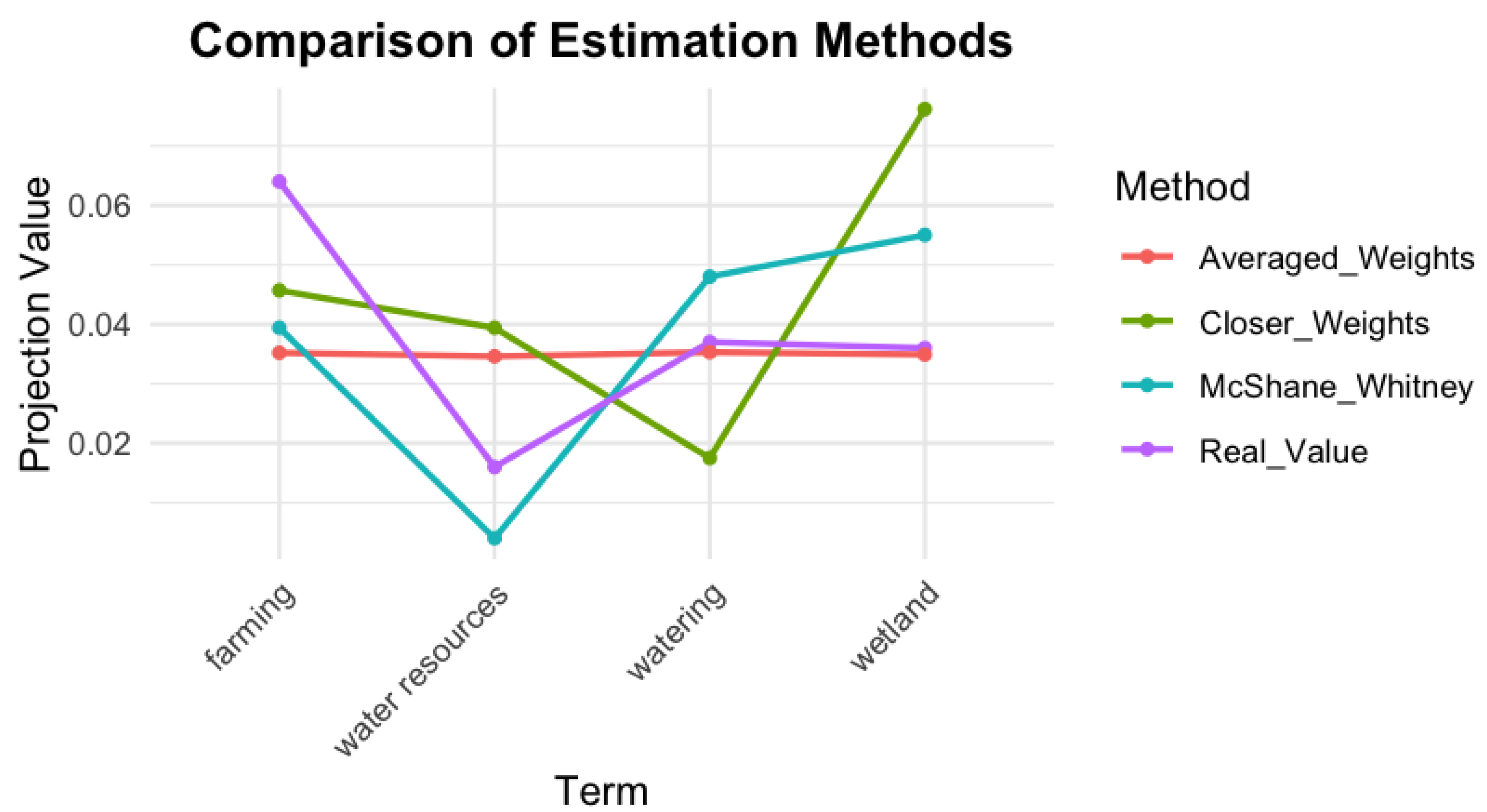
4.4.4. Evaluation Metrics and Analysis Procedures
These data are represented in
Figure 8. First, it is important to note that, due to the construction of the proposed methods, all estimates remain within the same value range as the original data. As shown, the method that best reproduces the trends observed in the real values is the McShane–Whitney extension, although the numerical accuracy is still limited. The Averaged Weights technique also provides a reasonably good approximation; however, the resulting values are rather uniform, which could be desirable if the goal is to obtain an average estimate of the representation of “rice” in the universe
based on the real values in
. Finally, and probably due to the fact that there are no large differences among the distances from “rice” to the other words in both universes
and
, the Closer Weights method produces the poorest results. A closer look at the construction process reveals that this technique assigns a disproportionately large weight to the nearest element, resulting in a strong deviation in contexts where all contributions are expected to be relatively similar.
The quadratic errors are presented in
Table 8, confirming through their numerical values the overall accuracy of the proposed estimation methods.
The example developed in this section shows how the proposed metric-based estimation methods behave when applied to a real semantic context. Although the agricultural example we used is relatively simple, it allows us to see important differences between the methods. The McShane–Whitney extension reproduces the overall trend of the real data more accurately, while the Averaged Weights method provides reasonable results, although more uniform and less sensitive to specific variations. The results of the Closer Weights method, however, is not as good, mainly because it relies too much on the nearest neighbor. This is not an appropriate strategy when distances between elements are all quite similar, as is the case in the example.
These results show that the choice of the estimation method should depend on the specific characteristics of the semantic universe and on what we want to achieve. If capturing fine differences between terms is important, methods like McShane–Whitney should be preferable. If a general average behavior is enough, the Averaged Weights method can work well.
4.5. Limitations and Future Directions
Although the examples we have shown can be reasonably interpreted as successful, the method we propose is still incomplete regarding the levels of reliability we can recognize in them. It depends heavily on how we can extract meaningful terms to initiate the analysis, how we can determine whether the universe of words we have fixed is broad enough to represent a semantic context, and how far we can trust the datasets, AI tools, and search engines for detecting the coincidences needed to compute the semantic projections.
The proposed technique includes elements that could be adapted to other contexts, as long as the assumptions about the occurrence of significant terms are maintained and the calculated ratios are sufficiently far from zero to avoid excessive sensitivity to small variations. However, its application to certain specific scenarios, such as the analysis of populations of certain insects in complex ecosystems (for which the number of related documents could be extremely small), would not be appropriate without further adjustments.
Thus, further investigations into AI instruments and the design of better tools for detecting relevant information in the databases must be carried out. Additionally, the construction and refinement of mathematical notions adapted to the problem would be necessary.
5. Conclusions
We have proposed a general analytical methodology for controlling the semantic projections of terms onto universes that describe a given semantic context. First, several statistical and AI methods are used to analyze how closely the semantic projections associated with different search methods (Google, Arxiv, DOAJ, and Google Scholar) align. This analysis allows us to decide, based on the experimental criteria, when any of the search procedures should be discarded.
Second, we present a methodology to compare universes that have been designed to represent the same semantic environments, using semantic projections and metric space tools. Our approach aims to evaluate how stable the description of a given semantic structure remains when different (but similar) universes are used to represent it. By developing and testing several estimation methods (weighted averages, closer-weight-based models, and Lipschitz extensions), we provide a flexible framework that can be adapted to different needs depending on the required degree of precision and sensitivity.
Through various examples in the agricultural context, we have firstly demonstrated a coherence analysis among different projection procedures, and secondly, we have shown how our techniques are capable of capturing both general trends and fine variations in the semantic relationships between terms. The McShane–Whitney extension, for instance, appears particularly useful when preserving subtle semantic differences is important, whereas the averaging methods offer a simpler approach that may be preferable in contexts where only a general approximation is sufficient.
Taken together, the two parts of this paper provide two complementary analytical tools that can help improve the study of contextual relationships across different descriptions of semantic environments. To enrich the discussion and provide a more prospective approach, it is worth considering the broader implications and possible future applications of the proposed framework. Beyond the application in the agricultural context we have explained, this methodology could be extended to other fields within Natural Language Processing (NLP) and Artificial Intelligence (AI). For example, it could be adapted to improve semantic analysis in specialized fields such as healthcare, legal studies, or environmental sciences, where understanding the nuanced relationships between terms is critical. In addition, the framework’s ability to compare and stabilize semantic representations across universes could be leveraged to improve multilingual PLN tasks such as machine translation or multilingual information retrieval, ensuring semantic consistency across languages.
Furthermore, the integration of this methodology with emerging AI tools, such as large linguistic models or knowledge graphs, could open new avenues for refining the semantic understanding and improving the interpretability of AI systems. For example, it could be used to validate or refine the semantic outputs of generative models, ensuring that they fit domain-specific contexts. The flexibility of the framework also suggests potential applications in dynamic environments, such as real-time data analysis or adaptive learning systems, where semantic relationships may evolve over time.


 ,
, 


