Assessing Expected Shortfall in Risk Analysis Through Generalized Autoregressive Conditional Heteroskedasticity Modeling and the Application of the Gumbel Distribution

Abstract

In this study, the Gumbel distribution is utilized to construct exact analytical representations for two pivotal measures in financial risk evaluation: Value at Risk (VaR) and Conditional Value at Risk (CVaR). These refined formulations are developed with the intention of offering resilient and practically implementable tools to address the complexities inherent in economic risk analysis. Moreover, the newly established expressions are seamlessly integrated into the GARCH modeling framework, thereby enriching its predictive capabilities. In order to verify both the practical relevance and theoretical soundness of the presented methodology, it is systematically employed regarding the daily return series of a varied portfolio of stocks. The outcomes of the numerical experiments provide compelling evidence of the approach’s reliability and effectiveness, emphasizing its suitability for advancing contemporary risk management strategies in financial environments.

1. Preliminaries and Background

The definition and interpretation of risk vary via the domain of application, with each perspective tailored to meet its specific objectives [1]. As highlighted by the Basel Committee about Banking Supervision (BCBS), economic institutions are obligated to maintain sufficient capital reserves to safeguard against expected damages arising from various risk sources during normal operations. These risks primarily include operational, market, and credit risks [2]. To achieve this, financial entities often assess the potential losses associated with their portfolios. This evaluation enables them to optimize fund allocation and effectively plan for investor payments [3].

Risk management is a cornerstone of modern finance, aiming to minimize potential losses under uncertain market conditions. Conditional Value at Risk (CVaR), i.e., Expected Shortfall (ES), is a robust risk quantifier that computes the average loss beyond a given confidence level [4,5]. Unlike VaR, which provides the loss threshold exceeded with a certain probability, ES offers deeper insight into tail risks, making it invaluable for managing extreme market events; see [6] for further discussions.

Within the realm of mathematical finance, one of the pioneering metrics for assessing risk is VaR. This measure, independently introduced by Markowitz [7] and Roy [8], provides a method to estimate the potential risk exposure of a portfolio while optimizing returns at predefined risk levels. VaR is mathematically expressed as follows [9]:

$${\mathrm{VaR}}_q\left(Y\right):=min\{z\in \mathbb{R}\mid G_Y\left(z\right)\ge q\},$$

(1)

where Y represents a variable subject to randomness, q is the predetermined confidence level, and $G_Y\left(·\right)$ denotes the cumulative distribution function (CDF). This formulation is versatile, accommodating both lower tails for losses (for instance, $q=1\%$) and upper tails for profits (for instance, $q=99\%$) by adjusting the tail level to q or $1-q$. While this study focuses on profits, the methodology is equally applicable to losses.

VaR provides insights into both the magnitude of potential losses and their associated probabilities. It is widely employed by banking institutions to evaluate the likelihood and extent of losses in their portfolios [10]. Additionally, selecting an appropriate risk measure is a critical factor in portfolio optimization as it allows for the scalarization and effective management of risk. For investments exhibiting consistent and stable performance over time, VaR proves to be adequate for risk management purposes [11]. However, its limitations become evident when stability is compromised as it fails to account for risks beyond its defined threshold. For example, the oil industry has demonstrated significant volatility in global oil prices since 2004, influenced by a multitude of factors.

To address these limitations, ES, also referred to as Average VaR (AVaR), serves as a complementary risk quantifier. ES quantifies the anticipated loss in the extreme tail of a distribution [12], offering a more comprehensive perspective on risk compared to VaR. It is formally defined as

$${\mathrm{ES}}_q\left(Y\right):=\mathbb{E}[Y\mid Y\ge {\mathrm{VaR}}_q\left(Y\right)],$$

(2)

where $\mathbb{E}$ denotes the conditional expectation of losses exceeding VaR.

Derived from VaR, ES is instrumental in optimizing portfolios and facilitating effective risk allocation. Risk allocation involves identifying, quantifying, and distributing risks appropriately among stakeholders. While risk cannot be entirely eliminated, accurately identifying and allocating it enables financial managers and stockholders to take informed actions to safeguard their capital. This proactive approach improves operational efficiency, enhances quality, minimizes delays, and fosters the resolution of disputes [13]. Notably, certain stock exchanges, such as the New York Stock Exchange (NYSE), mandate that listed companies compute and disclose their risk profiles using ES, thereby underscoring the significance and practicality of this risk assessment metric.

The expression provided in Definition (2) is often referred to as lower ES, or Tail VaR, when the inequality within the conditioned expectation includes equality. However, if the inequality is strict (excluding the equality condition), it is then identified as upper ES, which is sometimes alternatively known as ES [14].

An alternative formulation for ES, specifically tailored for continuous probability distributions, is provided in [15]

$${\mathrm{ES}}_q\left(Y\right):={\int }_{-\infty }^{\infty }zd{F}_Y^q\left(z\right),$$

(3)

where the q-tail distribution is characterized as

$$G_Y^q\left(z\right)=\left\{\begin{array}{ccc}0,\hfill & \hfill & z<{\mathrm{VaR}}_q\left(Y\right),\hfill \\ {\displaystyle \frac{G_Y\left(z\right)-q}{1-q}},\hfill & \hfill & z\ge {\mathrm{VaR}}_q\left(Y\right).\hfill \end{array}\right.$$

(4)

It is important to emphasize that the choice in distribution used for calculating VaR and ES significantly influences the estimation of the quartiles that define risk. Furthermore, achieving a closer fit between the empirical data and a particular type of distribution facilitates the development of functions that offer more accurate risk approximations under conditions characterized by volatility and uncertainty.

Generalized Autoregressive Conditional Heteroskedasticity (GARCH) processes are broadly utilized in financial econometrics to model and forecast volatility [16]. Since ES depends on both the distribution and volatility of returns, incorporating GARCH models enhances risk management by dynamically updating ES estimates based on changing market conditions [17]. This paper takes a different approach to attain the analytical formula for VaR and ES under the Gumbel distribution. Readers seeking broader context may consult [18] for supplementary discussions.

The approach adopted in this study builds upon the discussions found in Chapter 4.3 in [19] and [20,21], but it distinguishes itself by addressing key gaps. Unlike [19], this work explicitly provides analytical solutions for VaR and ES under the Gumbel distribution and directly applies them within the GARCH model to forecast risks associated with specific financial assets. The primary focus here is to utilize these derived formulas to evaluate the historic yields of various US market tickers, employing the GARCH framework.

This research emphasizes the importance of obtaining the solutions for VaR and ES using the Gumbel distribution. The significance lies in the historical evidence that poor risk management can lead to substantial financial losses within short timeframes. This study explores the precision of such risk quantifiers, comparing them with the Gumbel distribution in managing financial risks. The paper employs these formulas to simulate returns for prominent stocks over various time periods utilizing the GARCH process, as discussed in [22].

The organization of this work is outlined as follows. Section 2 and Section 3 review the principles and key characteristics of the background on ES and GARCH models, respectively. Section 4 furnishes an introduction to the Gumbel distribution and then derives an analytic formula for the VaR measure utilizing this distribution. The importance of innovation distribution is emphasized, particularly for analyzing both conditional and unconditional downside risks. Section 5 furnishes the derivation of the ES measure. Section 6 applies the derived formulations to compute VaR and ES, modeled using the GARCH(1,1) process. For further elaboration on related discussions, refer to [23]. Finally, Section 7 concludes the study by offering critical insights regarding the work.

2. Some Background on ES

The estimation of ES is contingent on the statistical properties of portfolio returns. Several approaches are commonly employed as follows:

• Parametric Methods: These approaches assume that returns follow a specific distribution, like the normal or Student’s t distributions. The ES is computed using analytical formulas derived from the CDF.
• Non-Parametric Methods: These methods do not rely on distributional assumptions and use empirical data. For example, the historical simulation approach sorts past returns and averages the worst $100\times (1-q)\%$ of losses to estimate ES.
• Monte Carlo Simulations: These involve generating a large number of hypothetical portfolio returns via a stochastic model and computing ES from the simulated distribution. This method is particularly effective for capturing complex dependencies in asset returns.

3. GARCH Models

Numerous studies (e.g., Ref. [24] and the references therein) have demonstrated the critical role of forecasting future variance using advanced GARCH-type models for effectively managing portfolio risk. This necessity arises from the inherent presence of heteroskedasticity, characterized by non-constant volatility in the underlying financial processes under consideration.

Volatility, defined as the square root of the conditioned variance of the logarithmic process of return, depends on the information available up to the previous time step. Mathematically, this is expressed using ${\mathcal{F}}_{t-1}$, the $\sigma$-algebra generated by the sequence of observations $x_0,x_1,\dots ,x_{t-1}$. Consequently, if $p_t$ represents the price of a stock at time t on a stock exchange, the logarithmic returns can be defined as follows [25]:

$$x_t=-log{p}_{t-1}+log{p}_t.$$

(5)

Additionally, it is possible to characterize

$${\sigma }_t^2=\mathrm{Var}\left[x_t^2\right|{\mathcal{F}}_{t-1}].$$

(6)

To demonstrate the practical applicability of the presented explicit risk quantifiers derived under the Gumbel distribution using the GARCH framework, it is first essential to revisit the concept of the GARCH process. This model, fundamentally an ARMA process applied to the variance of errors, has been widely studied and utilized in financial modeling, as discussed in [25].

In a GARCH($p_1$,$p_2$) model, the parameter $p_1$ represents the order of the GARCH components, denoted by ${\sigma }^2$, whereas $p_2$ signifies the order of the ARCH components, denoted by ${ϵ}^2$. For the purpose of this study, we focus specifically on the GARCH(1,1) model, expressed as follows ($r_t$ refers to the actual return):

$$\begin{array}{c}\hfill \begin{array}{cc}\hfill r_t=& \varrho +{\epsilon }_t=\varrho +{\sigma }_t{z}_t,\hfill \\ \hfill {\sigma }_t^2=& w+\lambda {\epsilon }_{t-1}^2+\beta {\sigma }_{t-1}^2,\hfill \end{array}\end{array}$$

(7)

where $z_t$ represents a stochastic component, characterized as independent and identically distributed (i.i.d.) samples with a mean of zero and unit variance. In this context, $w>0$ denotes a constant term, $\varrho$ signifies the expected return, and ${\sigma }_t$ corresponds to the volatility of the yields on a given t. Additionally,

$$\beta +\lambda <1,\beta \ge 0,\lambda \ge 0.$$

(8)

The relation $\beta +\lambda <1$ in (8) ensures the existence of a stationary resolution for the GARCH process.

The process in (7) has found widespread application in the modeling of economical time series and has been integrated into numerous econometric and statistical software packages, as noted in [26]. Its popularity among practitioners stems from its straightforward implementation compared to other stochastic volatility (SV) models. Additionally, financial data are typically reported in discrete intervals, making this model more practical for such datasets, as discussed in [27,28].

One of the notable strengths of GARCH-like processes is their ability to capture both the fat-tailed nature of financial return distributions and the phenomenon of volatility clustering. As established in [29], the stationary resolution of a GARCH(1,1) model exhibits heavy-tail characteristics. Consequently, GARCH-like processes serve as highly effective tools in risk management, providing robust frameworks for understanding and forecasting market behavior.

For instance, consider a GARCH(1,1) model for return volatility:

$${\sigma }_t^2=\omega +q_1{r}_{t-1}^2+\beta {\sigma }_{t-1}^2,$$

(9)

where ${\sigma }_t^2$ is the conditional variance, $r_{t-1}$ is the lagged return, and $\omega$, $q_1$, and $\beta$ are model parameters. By plugging the time-varying volatility ${\sigma }_t$ into the parametric ES formula, we obtain a more accurate measure of tail risk that adapts to market dynamics.

Assume a portfolio with returns following a normal distribution (here with its two parameters, $a=0$ and $b=0.02$). At a 95% confidence level ($q=0.95$), the ES using the parametric method is

$${\mathrm{ES}}_{0.95}=0.02\times {\displaystyle \frac{\varphi \left({\Phi }^{-1}\left(0.95\right)\right)}{1-0.95}}\approx 0.033.$$

This estimate can be refined by using a GARCH model to forecast ${\sigma }_t$, allowing for time-varying risk management strategies.

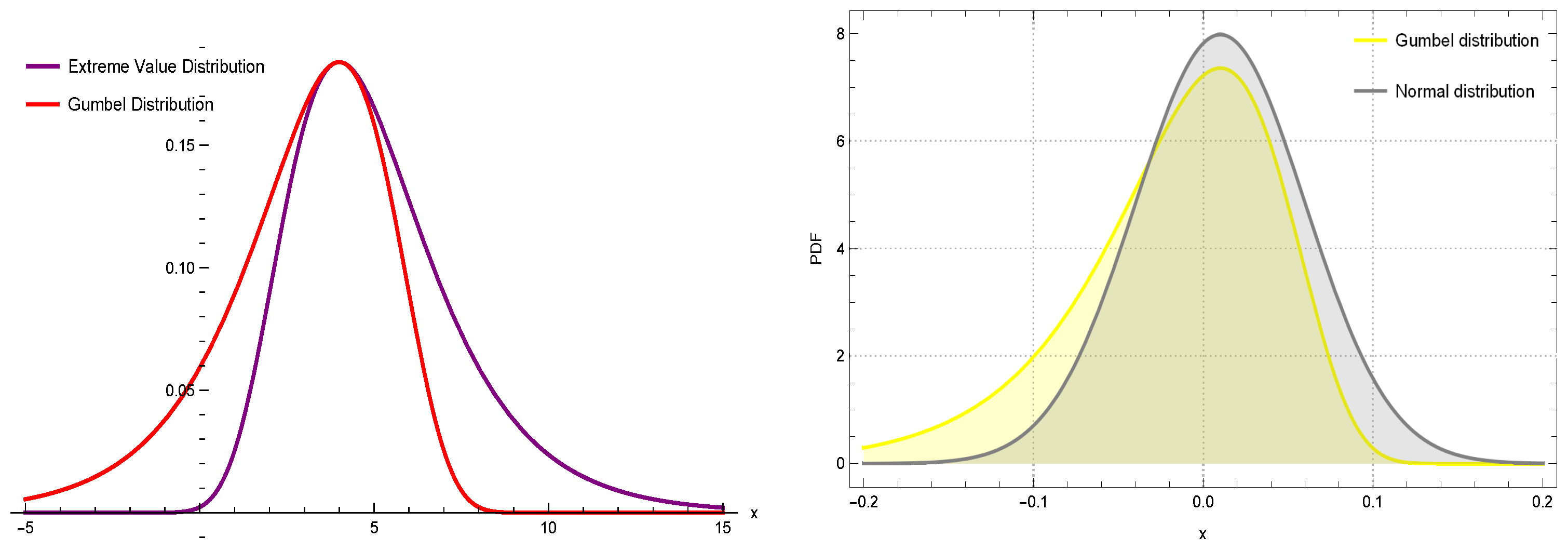
4. VaR Based on the Gumbel Distribution

The Gumbel distribution [30] is particularly fruitful in the context of extreme events, where interest is placed on modeling the behavior of the largest observed values in a series.

The PDF of the Gumbel distribution can be provided as [31]

$$g\left(x\right)={\displaystyle \frac{e^{\frac{x-a}{b}-e^{\frac{x-a}{b}}}}{b}},$$

(10)

where

• $x\in \mathbb{R}$;
• a is the parameter of location, which shifts the distribution along the x-axis;
• $b>0$ is the parameter of scale, which specifies the spread of the distribution.

The CDF of the distribution of Gumbel is

$$G\left(x\right)=1-e^{-e^{\frac{x-a}{b}}}.$$

(11)

Here, we use the Gumbel distribution with the CDF function of the commonly used form $1-e^{-e^{\frac{x-a}{b}}}$ and not the standard form $e^{-e^{(-x)}}$ [32]. This is mainly because we followed the definitions given in [31]. The Gumbel distribution is particularly valuable in disaster risk management due to its ability to model extreme events, such as natural disasters, which tend to occur with low probability but can have severe impacts. The key feature of the Gumbel distribution is its focus on extreme values, which are critical in disaster planning and risk assessment. See Figure 1 and Figure 2 referring to different cases of Gumblel distribution for the PDF and CDF and their comparisons to other distributions.

For instance, consider a scenario where historical data are available on the maximum annual river levels over the past ten years. The Gumbel distribution can be applied to model the probability of future extreme river levels, thereby providing insight into the likelihood of floods. Specifically, the distribution helps in estimating the return period of extreme events, which refers to the average time between events of a certain severity. For example, a 100-year flood corresponds to an event that has a 1% chance of occurring in any given year. The Gumbel distribution can be used to estimate this return period based on the observed data, thus aiding in flood risk management.

The Gumbel distribution is often applicable when the underlying data are from a normal or exponential distribution, making it an ideal choice for modeling the distribution of extreme natural disasters.

Let us consider the case of river flood management. Suppose the annual maximum river levels over the past ten years are given as follows (in meters):

$$[5.2, 6.0, 5.7, 5.5, 6.2, 5.9, 6.3, 5.8, 6.1, 5.4].$$

The sample mean and standard deviation are computed as $a=5.85$ and $b=0.3$, respectively. Assuming the river levels approximately follow a Gumbel distribution, we can estimate the 100-year flood level, which corresponds to the 1% quantile ($q=0.01$) of the distribution. Using the formula for the inverse CDF of the Gumbel distribution, we can calculate the extreme value threshold corresponding to this return period:

$$x_{0.01}=a-\beta ln(-ln\left(q\right))=5.85-0.3ln(-ln\left(0.01\right))\approx 6.91\mathrm{m}.$$

(12)

Thus, the 100-year flood level is estimated to be approximately 6.91 m.

Now, we have the following continuous stochastic variable:

$$Y\sim \mathrm{Gumbel}\mathrm{distribution}(a,b).$$

(13)

Throughout this study, the notation log consistently refers to the natural logarithm. Two critical parameters in the analysis are T and q, both of which are selected with precision based on the specific objectives of the risk management task at hand, whether it pertains to regulatory compliance, corporate risk assessment, or other strategic goals.

Theorem 1.

Assume $Y\in L^p$ represents a variable with randomness modeling loss under the Gumbel distribution(a, b). The VaR quantifier for Y is expressible in a closed-form formula as given in (16).

Proof. 

In this context, the random variable Y belongs to the $L^p$ space, which is a class of function spaces (also known as Lebesgue spaces). Using the relation provided in (1), we derive

$$\begin{array}{cc}\hfill {\mathrm{VaR}}_q\left(Y\right)& =min\{z\in \mathbb{R}|p(Y\le z)\ge q\},\hfill \end{array}$$

(14)

$$\begin{array}{cc}\hfill & \hspace{1em}\hspace{1em}=min\{z\in \mathbb{R}|G_Y\left(z\right)\ge q\},\hfill \end{array}$$

(15)

$$\begin{array}{cc}\hfill & \hspace{1em}\hspace{1em}=a+blog(-log(1-q\left)\right).\hfill \end{array}$$

(16)

This completes the proof.    □

It has been observed that the Gumbel distribution provides adaptability for modeling financial and economic data compared to the widely utilized normal distribution.

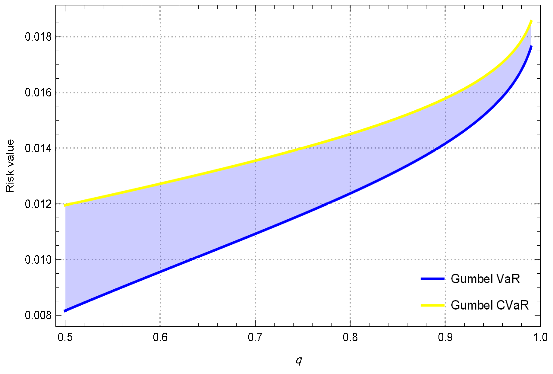
5. ES via the Gumbel Distribution

As previously discussed, the VaR quantifies the maximum potential loss over a specified timeframe at q. However, the ES extends this analysis by measuring the average loss incurred when the VaR threshold is breached. Essentially, ES estimates the expected losses after the VaR breakpoint.

Theorem 2.

Given the conditions specified in Theorem 1, the ES corresponding to the Gumbel distribution can be formulated analytically, as shown in Equation (20).

Proof. 

Adopting a comparable approach to that employed in Theorem 1 and applying the definition stated in (2), we derive

$$\begin{array}{cc}\hfill {\mathrm{ES}}_q\left(Y\right)& =\mathbb{E}\left[Y|{\mathrm{VaR}}_q\left(Y\right)\le Y\right],\hspace{1em}\hspace{1em}\hspace{1em}\hspace{1em}\hspace{1em}\hspace{1em}\hspace{1em}\hspace{1em}\hspace{1em}\hfill \end{array}$$

(17)

$$\begin{array}{cc}\hfill & =\mathbb{E}\left[Y|a-blog(-log\left(q\right))\le Y\right],\hspace{1em}\hspace{1em}\hspace{1em}\hfill \end{array}$$

(18)

$$\begin{array}{cc}\hfill & \hspace{1em}\hspace{1em}\hspace{1em}\hspace{1em}\hspace{1em}\hspace{1em}\hspace{1em}\hspace{1em}\hspace{1em}\hspace{1em} ={\displaystyle \frac{aq-a+b\mathrm{li}(1-q)-blog(-log(1-q\left)\right)+bqlog(-log(1-q\left)\right)}{q-1}},\hfill \end{array}$$

(19)

$$\begin{array}{cc}\hfill & =a+{\displaystyle \frac{b\mathrm{li}(1-q)}{q-1}}+blog(-log(1-q)),\hfill \end{array}$$

(20)

wherein the logarithmic integral map is expressed as

$$\mathrm{li}\left(\varpi \right)={\int }_0^{\varpi }{\displaystyle \frac{1}{log\left(\delta \right)}}d\delta .$$

(21)

The transition from (18) to (19) is conducted based on severe simplifications and symbolic computations occurring in (18). This completes the proof.    □

Figure 3 illustrates the connection between VaR and ES. Based on the numerical comparisons provided in

Table 1. The ES and VaR across normal and Gumbel distributions with varying parameters.

a	b	q	VaR  (Normal)	VaR (Gumbel Distribution)	ES  (Normal)	ES (Gumbel  Distribution)
0.020	0.0020	0.85	0.022	0.021	0.023	0.022
0.020	0.0020	0.90	0.023	0.022	0.024	0.022
0.020	0.0020	0.95	0.023	0.022	0.024	0.023
0.020	0.0040	0.85	0.024	0.023	0.026	0.024
0.020	0.0040	0.90	0.025	0.023	0.027	0.025
0.020	0.0040	0.95	0.027	0.024	0.028	0.025
0.020	0.0060	0.85	0.026	0.024	0.029	0.026
0.020	0.0060	0.90	0.028	0.025	0.031	0.027
0.020	0.0060	0.95	0.030	0.027	0.032	0.028
0.020	0.0080	0.85	0.028	0.025	0.032	0.028
0.020	0.0080	0.90	0.030	0.027	0.034	0.029
0.020	0.0080	0.95	0.033	0.029	0.037	0.031
0.040	0.0020	0.85	0.042	0.041	0.043	0.042
0.040	0.0020	0.90	0.043	0.042	0.044	0.042
0.040	0.0020	0.95	0.043	0.042	0.044	0.043
0.040	0.0040	0.85	0.044	0.043	0.046	0.044
0.040	0.0040	0.90	0.045	0.043	0.047	0.045
0.040	0.0040	0.95	0.047	0.044	0.048	0.045
0.040	0.0060	0.85	0.046	0.044	0.049	0.046
0.040	0.0060	0.90	0.048	0.045	0.051	0.047
0.040	0.0060	0.95	0.050	0.047	0.052	0.048
0.040	0.0080	0.85	0.048	0.045	0.052	0.048
0.040	0.0080	0.90	0.050	0.047	0.054	0.049
0.040	0.0080	0.95	0.053	0.049	0.057	0.051
0.060	0.0020	0.85	0.062	0.061	0.063	0.062
0.060	0.0020	0.90	0.063	0.062	0.064	0.062
0.060	0.0020	0.95	0.063	0.062	0.064	0.063
0.060	0.0040	0.85	0.064	0.063	0.066	0.064
0.060	0.0040	0.90	0.065	0.063	0.067	0.065
0.060	0.0040	0.95	0.067	0.064	0.068	0.065
0.060	0.0060	0.85	0.066	0.064	0.069	0.066
0.060	0.0060	0.90	0.068	0.065	0.071	0.067
0.060	0.0060	0.95	0.070	0.067	0.072	0.068
0.060	0.0080	0.85	0.068	0.065	0.072	0.068
0.060	0.0080	0.90	0.070	0.067	0.074	0.069
0.060	0.0080	0.95	0.073	0.069	0.077	0.071
0.080	0.0020	0.85	0.082	0.081	0.083	0.082
0.080	0.0020	0.90	0.083	0.082	0.084	0.082
0.080	0.0020	0.95	0.083	0.082	0.084	0.083
0.080	0.0040	0.85	0.084	0.083	0.086	0.084
0.080	0.0040	0.90	0.085	0.083	0.087	0.085
0.080	0.0040	0.95	0.087	0.084	0.088	0.085
0.080	0.0060	0.85	0.086	0.084	0.089	0.086
0.080	0.0060	0.90	0.088	0.085	0.091	0.087
0.080	0.0060	0.95	0.090	0.087	0.092	0.088
0.080	0.0080	0.85	0.088	0.085	0.092	0.088
0.080	0.0080	0.90	0.090	0.087	0.094	0.089
0.080	0.0080	0.95	0.093	0.089	0.097	0.091

, the results reveal that ES under the Gumbel distribution provides mostly lower or equal scalarized risk values in contrast to VaR, as expected theoretically. The experimental pieces of evidence presented in Table 1 demonstrate that better risk values can be predicted through the application of VaR and ES utilizing the Gumbel distribution, which exhibit greater values compared to the conventional normal distribution. This enhances investor confidence in trading, especially during sudden price movements in stocks that may lead to substantial gains or losses. The findings also suggest that increased risk budgets are sufficient, ensuring that risks are not excessively overestimated, thereby avoiding overcautious trading behavior.

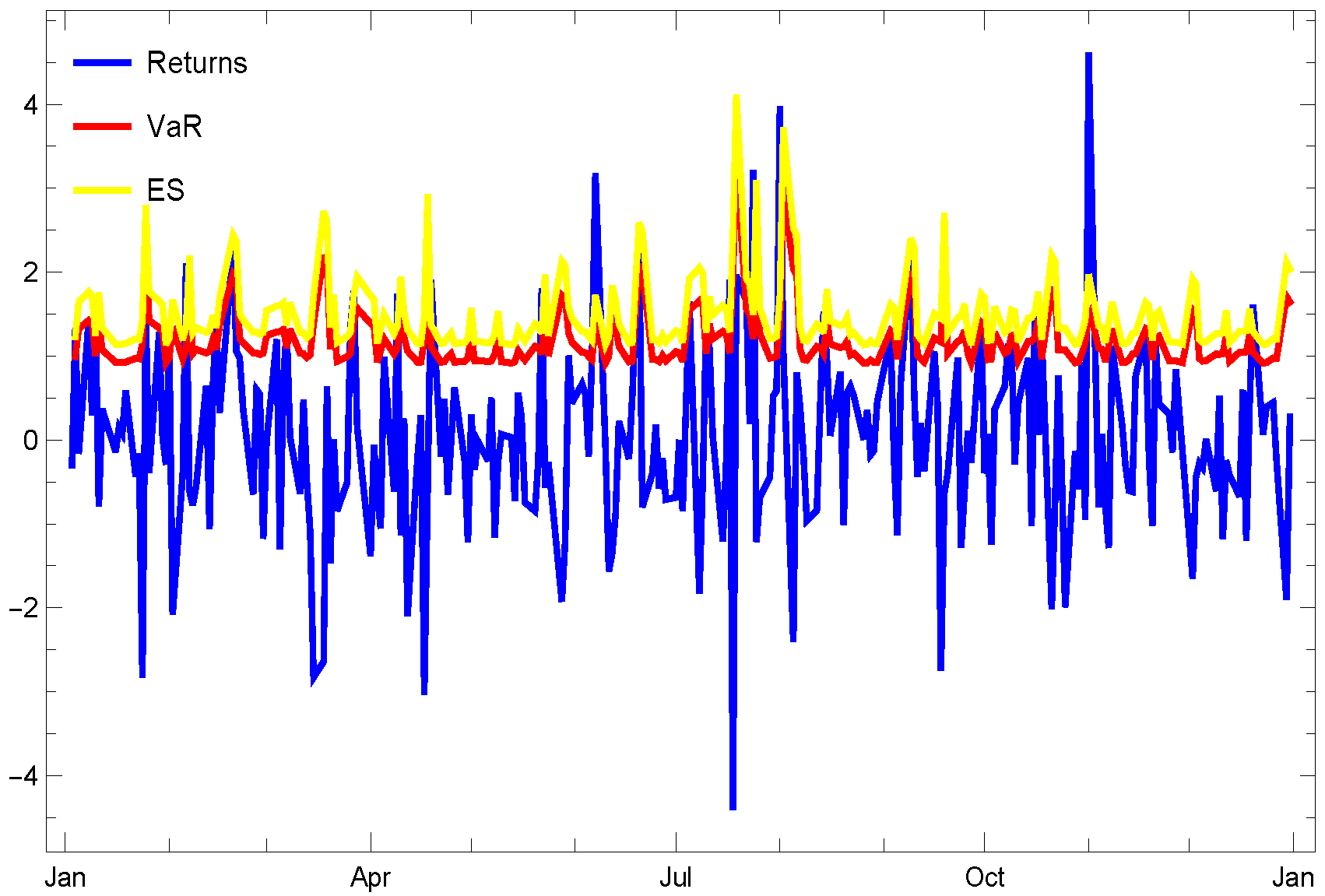
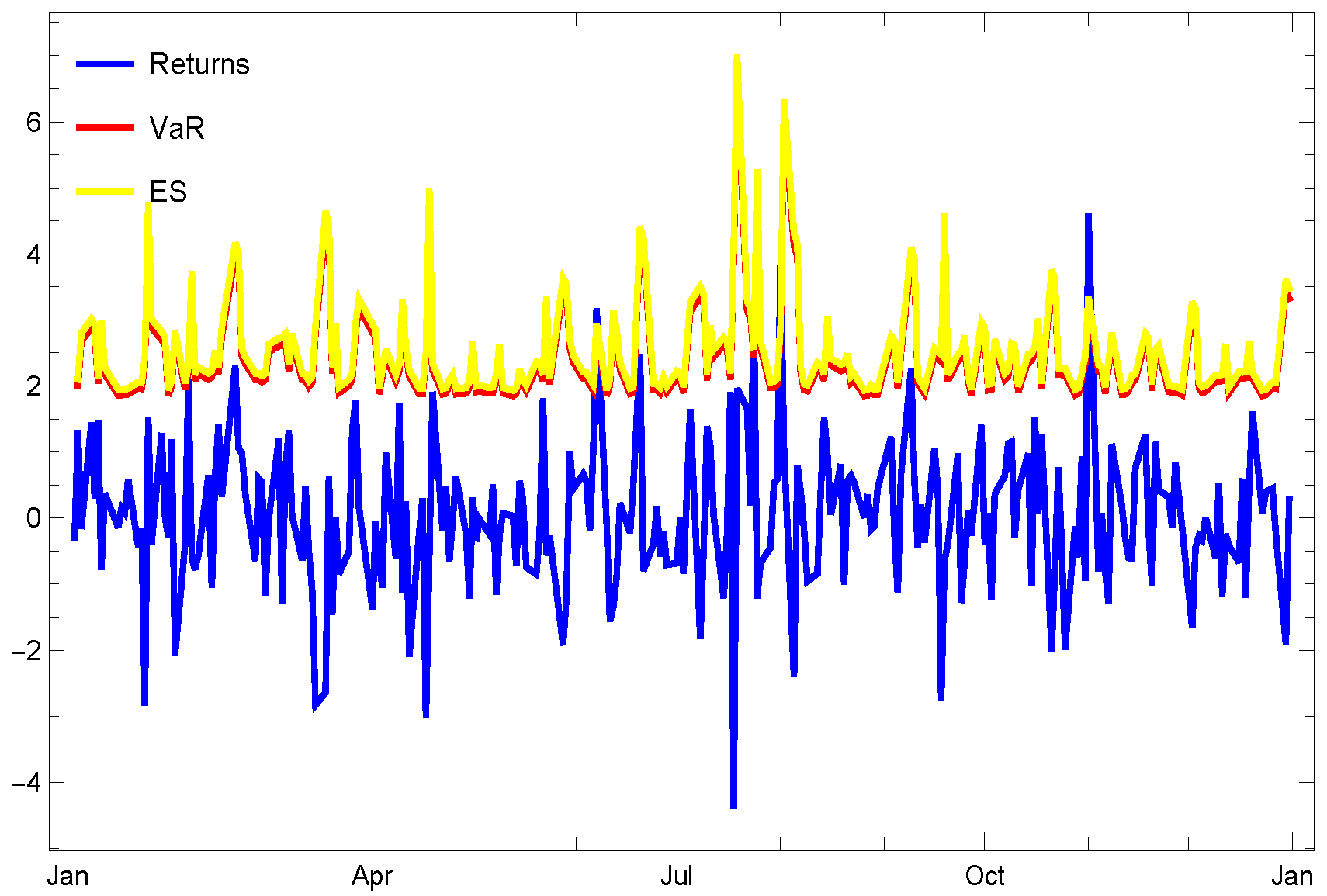
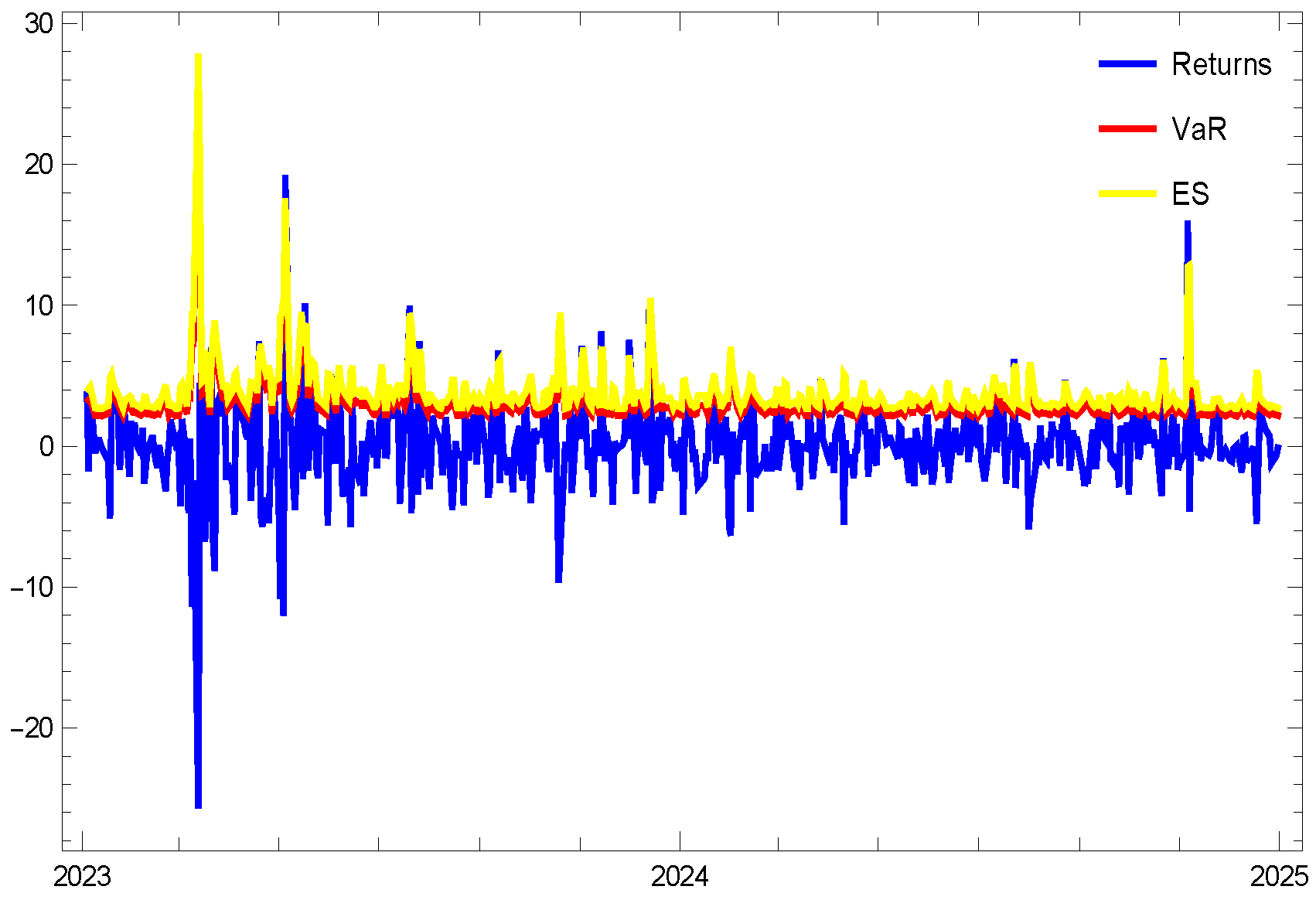
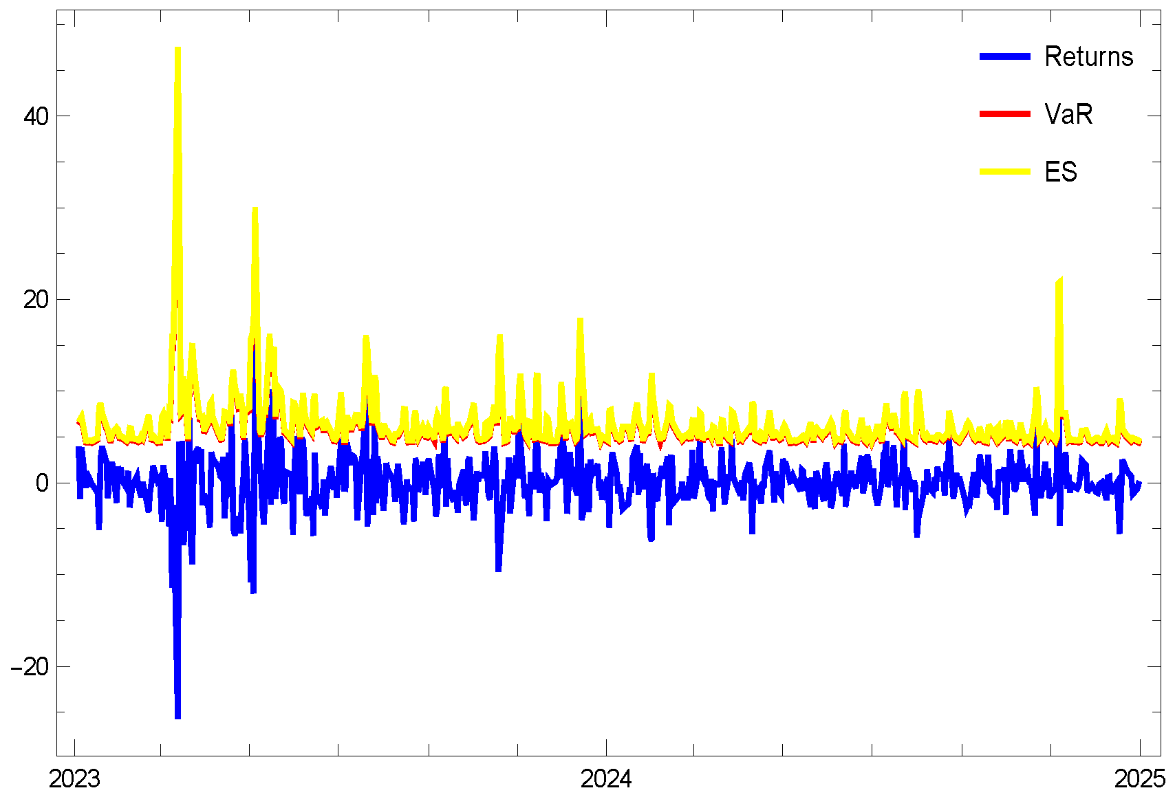
6. Numerical Validations

The purpose here is to evaluate VaR and ES forecasts using the GARCH model to manage risk for trading days in an equity market primarily drawn from S&P500. The data selected aim to represent a variety of stocks. For the assessment of the risk measures, a 1-day-ahead volatility forecast methodology is employed. All computations were conducted in Mathematica 13.3 [33] using machine precision. We assume that $z_t$ in (7) has the centered normalized Gumbel distribution.

The stocks considered in this study are as follows:

• The 1st experiment involves the stock ticker “NYSE:ABT”.
• The 2nd test focuses on “NASDAQ:ZION”.

The details for the tickers and the associated data are presented in

Table 2. The characteristics of the selected market tickers.

Stock	Tickers	Market	Section	Float Shares	Starting	Ending	Data Size
Abbott Laboratories	NYSE:ABT	NYSE	Medical Devices	1734455940	1 January 2024	1 January 2025	251
Zions Bancorp NA	NASDAQ:ZION	NASDAQ	Banks Regional	147699000	1 January 2023	1 January 2025	501

. Here, data size stands for the size of the data in the business days of the given time window, i.e., the number of days in which we have the stock prices and are able to compute the returns and then calculate the best fit based on the GARCH process.

By utilizing the model defined in (7) to analyze the stock returns through fitting a temporal series methodology [34], the resulting characteristics are presented in

Table 3. The parameter estimates obtained from fitting the GARCH(1,1) model to the data in the 1st test.

w	$\mathit{\lambda }$	$\mathit{\beta }$	The Variance for Error
0.696408	0.426945	0.0481203	6.49298

and

Table 4. The parameter estimates obtained from fitting the GARCH(1,1) model to the data in the 2nd test.

w	$\mathit{\lambda }$	$\mathit{\beta }$	The Variance for Error
3.83852	0.304459	0.323751	1241.83

employing maximum likelihood approach for the process estimator. To reveal how we combine the GARCH(1,1) and risk measures, we provide some of our written codes in Mathematica 13.0 environment for this task using (16) and (20) as follows:

modelfit = TimeSeriesModelFit[return, ``GARCH’’,

  ProcessEstimator -> ``MaximumLikelihood’’]

par = modelfit[``BestFit’’]

gvol = MovingMap[StandardDeviation, return, 4];

gVaRfn = (16) /. {a -> 0,

    b -> Sqrt[par[[1]] + par[[2, 1]] x^2 + par[[3, 1]] y^2]};

cVaRfn = (20) /. {a -> 0,

    b -> Sqrt[par[[1]] + par[[2, 1]] x^2 + par[[3, 1]] y^2]};

comb = Quiet@TimeSeriesThread[QuantityMagnitude, {return, gvol}];

Here, in the written codes, $\mathtt{par}$ and $\mathtt{return}$ stand for the best fit in the command $\mathtt{TimeSeriesModelFit}\left[\right]$ and the stock fractional changes, respectively.

The numerical findings from the simulations presented in Figure 4, Figure 5, Figure 6 and Figure 7 for the initial test reveal the following insights:

• Firstly, as the pre-specified tail level increases, both risk measures progressively converge toward one another.
• Selecting a pre-specified confidence level of $99.99\%$ appears to be a prudent selection for analyzing highly volatile stocks, particularly when employing these risk measures under the Gumbel distribution.

It is worth noting that numerous previous methodologies have relied on the assumption of normality or log-normality [35]. While the Gumbel distribution exhibits a relatively thin tail on the right side of its PDF, the choice in the confidence level of $99.99\%$ can produce robust risk assessments and reliable scalar values in financial markets.

7. Conclusions

The ES has proven to be instrumental in assessing worst-case scenarios for investment portfolios, particularly in addressing concerns related to tail events, such as major natural disasters or economic shocks. It has also been employed in underwriting decisions to determine appropriate capital reserves. The Gumbel distribution has provided a fundamental framework for modeling the distribution of extreme values, establishing itself as a crucial tool in disaster risk management. By offering robust insights into the likelihood of catastrophic events, it has facilitated the development of strategies aimed at mitigating their impact on communities and infrastructure. In this study, we have utilized the Gumbel distribution to derive explicit analytical expressions for two widely recognized risk measures, namely VaR and ES. These refined formulas have been designed to serve as effective tools for economic risk management. Furthermore, the derived formulations have been integrated into the GARCH model framework. To validate the theoretical framework developed in this study, we have applied the proposed approach to daily returns from a selection of stocks.

References

1. Albrecher, H.; Binder, A.; Lautscham, V.; Mayer, P. Introduction to Quantitative Methods for Financial Markets; Springer: Basel, Switzerland, 2013. [Google Scholar]
2. Bormetti, G.; Cisana, E.; Montagna, G.; Nicrosini, O. A non-Gaussian approach to risk measures. Physica A 2007, 376, 532–542. [Google Scholar] [CrossRef]
3. Galindo, J.; Tamayo, P. Credit risk assessment using statistical and machine learning basic methodology and risk modeling applications. Comput. Econ. 2000, 15, 107–143. [Google Scholar] [CrossRef]
4. Wang, G.-J.; Zhu, C.-L. BP-CVaR: A novel model of estimating CVaR with back propagation algorithm. Econ. Lett. 2021, 209, 110125. [Google Scholar] [CrossRef]
5. Martín, J.; Isabel Parra, M.; Pizarro, M.M.; Sanjuán, E.L. A new Bayesian method for estimation of value at risk and conditional value at risk. Empir. Econ. 2024, 68, 1171–1189. [Google Scholar] [CrossRef]
6. Ahmed, D.; Soleymani, F.; Ullah, M.Z.; Hasan, H. Managing the risk based on entropic value-at-risk under a normal-Rayleigh distribution. Appl. Math. Comput. 2021, 402, 126129. [Google Scholar] [CrossRef]
7. Markowitz, H. Portfolio selection. J. Financ. 1952, 7, 77–91. [Google Scholar]
8. Roy, A. Safety first and the holding of assets. Econometrica 1952, 20, 431–449. [Google Scholar] [CrossRef]
9. Lechner, L.A.; Ovaert, T.C. Value-at-risk: Techniques to account for leptokurtosis and asymmetric behavior in returns distributions. J. Risk Financ. 2010, 11, 464–480. [Google Scholar] [CrossRef]
10. Benninga, S.; Wiener, Z. Value-at-Risk (VaR). Math. Edu. Res. 1998, 7, 1–8. [Google Scholar]
11. Braione, M.; Scholtes, N.K. Forecasting value-at-risk under different distributional assumptions. Econometrics 2016, 4, 3. [Google Scholar] [CrossRef]
12. Wang, Z.-R.; Chen, Y.-H.; Jin, Y.-B.; Zhou, Y.-J. Estimating risk of foreign exchange portfolio: Using VaR and CVaR based on GARCH-EVT-Copula model. Phys. A 2010, 389, 4918–4928. [Google Scholar] [CrossRef]
13. Soleymani, F.; Itkin, A. Pricing foreign exchange options under stochastic volatility and interest rates using an RBF-FD method. J. Comput. Sci. 2019, 37, 101028. [Google Scholar] [CrossRef]
14. Sarykalin, S.; Serraino, G.; Uryasev, S. Value-at-risk vs. conditional value-at-risk in risk management and optimization. In State-of-the-Art Decision-Making Tools in the Information-Intensive Age; Tutorials in Operations Research; Informs: Catonsville, MD, USA, 2008; pp. 270–294. [Google Scholar]
15. Rockafellar, R.T.; Uryasev, S. Conditional value-at-risk for general loss distributions. J. Bank. Financ. 2002, 26, 1443–1471. [Google Scholar] [CrossRef]
16. Herwartz, H. Stock return prediction under GARCH—An empirical assessment. Int. J. Forecast. 2017, 33, 569–580. [Google Scholar] [CrossRef]
17. Norton, M.; Khokhlov, V.; Uryasev, S. Calculating CVaR and bPOE for common probability distributions with application to portfolio optimization and density estimation. Ann. Oper. Res. 2021, 299, 1281–1315. [Google Scholar] [CrossRef]
18. Goode, J.; Kim, Y.S.; Fabozzi, F.J. Full versus quasi MLE for ARMA-GARCH models with infinitely divisible innovations. Appl. Econ. 2015, 47, 5147–5158. [Google Scholar] [CrossRef]
19. McNeil, Q.J.; Frey, R.; Embrechts, P. Quantitative Risk Management, Revised ed.; Princeton University Press: Princeton, NJ, USA, 2015. [Google Scholar]
20. Viet Long, H.; Bin Jebreen, H.; Dassios, I.; Baleanu, D. On the statistical GARCH model for managing the risk by employing a fat-tailed distribution in finance. Symmetry 2020, 12, 1698. [Google Scholar] [CrossRef]
21. Ullah, M.Z.; Mallawi, F.O.; Asma, M.; Shateyi, S. On the conditional value at risk based on the laplace distribution with application in GARCH model. Mathematics 2022, 10, 3018. [Google Scholar] [CrossRef]
22. Williams, B. GARCH(1, 1) Models; Ruprecht-Karls-Universität Heidelberg: Heidelberg, Germany, 2011. [Google Scholar]
23. De-Graft, E.; Owusu-Ansah, J.; Barnes, B.; Donkoh, E.K.; Appau, J.; Effah, B.; Mccall, M. Quantifying economic risk: An application of extreme value theory for measuring fire outbreaks financial loss. Financ. Math. Appl. 2019, 4, 1–12. [Google Scholar]
24. Halkos, G.E.; Tsirivis, A.S. Value-at-risk methodologies for effective energy portfolio risk management. Econ. Anal. Policy 2019, 62, 197–212. [Google Scholar] [CrossRef]
25. Bollerslev, T. Generalized autoregressive conditional heteroskedasticity. J. Econometr. 1986, 31, 307–327. [Google Scholar] [CrossRef]
26. Hlivka, I. VaR, CVaR and Their Time Series Applications; Research Note; Quant Solutions Group: London, UK, 2015; pp. 1–2. [Google Scholar]
27. Chu, J.; Chan, S.; Nadarajah, S.; Osterrieder, J. GARCH Modelling of Cryptocurrencies. J. Risk Financ. Manag. 2017, 10, 17. [Google Scholar] [CrossRef]
28. Echaust, K.; Just, M. Value at risk estimation using the GARCH-EVT approach with optimal tail selection. Mathematics 2020, 8, 114. [Google Scholar] [CrossRef]
29. Davis, R.A.; Mikosch, T. Extreme value theory for GARCH processes. In Handbook of Financial Time Series; Springer: Berlin/Heidelberg, Germany, 2009; pp. 187–200. [Google Scholar]
30. Gumbel, E.J. Les valeurs extrêmes des distributions statistiques (PDF). Ann. L’Institut Henri Poincaré 1935, 5, 115–158. [Google Scholar]
31. Available online: https://reference.wolfram.com/language/ref/GumbelDistribution.html.en (accessed on 4 October 2016).
32. Gumbel, E.J. The return period of flood flows. Ann. Math. Stat. 1941, 12, 163–190. [Google Scholar] [CrossRef]
33. Georgakopoulos, N.L. Illustrating Finance Policy with Mathematica; Springer International Publishing: London, UK, 2018. [Google Scholar]
34. Soleymani, F.; Ma, Q.; Liu, T. Managing the risk via the Chi-squared distribution in VaR and CVaR with the use in generalized autoregressive conditional heteroskedasticity model. Mathematics 2025, 13, 1410. [Google Scholar] [CrossRef]
35. Engle, R.F. Autoregressive conditional heteroskedasticity with estimates of the variance of U.K. inflation. Econometrica 1982, 50, 987–1008. [Google Scholar] [CrossRef]
Figure 1. The PDF a = 0 and CDF a = 2 for the Gumbel distribution, left and right, respectively.
Axioms 14 00391 g001
Figure 2. The PDFs of Gumbel and extreme-value distributions (left) under a = 4 and b = 2 and the PDFs of Gumbel and normal distributions (right) under a = 0.01 and b = 0.05 .
Axioms 14 00391 g002
Figure 3. A comparative evaluation of VaR and ES is carried out based on Theorems 1 and 2, with parameters a = 0.01 and b = 0.005 .
Axioms 14 00391 g003
Figure 4. The comparative analysis of the risk quantifiers is performed for the pre-specified tail level, with α = 95 % focusing on the 1st test.
Axioms 14 00391 g004
Figure 5. The comparative analysis of the risk quantifiers is performed for the pre-specified tail level, with α = 99.99 % depicted on the right, focusing on the 1st test.
Axioms 14 00391 g005
Figure 6. The comparative analysis of the risk quantifiers is performed for the pre-specified tail level, with α = 95 % focusing on the 2nd test.
Axioms 14 00391 g006
Figure 7. A comparison of the risk measures conducted at α = 99.99 % is illustrated, emphasizing the second test case.
Axioms 14 00391 g007