An Enhanced Method with Memory Derived from Newton’s Scheme in Solving Nonlinear Equations: Higher R-Order Convergence and Numerical Performance

Abstract

This article introduces a novel iterative solver with memory, derived from Newton’s scheme, for nonlinear scalar equations. The key innovation lies in integrating memory into the iterative process, enhancing the convergence rate without increasing the quantity of functional evaluations compared to conventional two-point solvers. The proposed method achieves a superior R-order of convergence by adaptively utilizing past iterates to refine the current approximation. A rigorous theoretical analysis is presented to establish the convergence properties of the method. Extensive computational experiments demonstrate that the method with memory not only accelerates convergence but also enhances accuracy with fewer iterations. These findings suggest that the proposed solver has significant potential for applications in scientific computing and numerical optimization, where efficient and high-order iterative methods are crucial.

1. Introductory Notes

Solving nonlinear scalar equations is fundamental in numerous scientific and engineering disciplines, as many real-world problems involve nonlinear behavior that cannot be accurately captured by linear models [1,2,3]. These equations frequently arise in physics, engineering, economics, and biology, where exact analytical solutions are often unavailable [4,5]. In physics and engineering, nonlinear equations govern the behavior of complex systems such as fluid dynamics, structural mechanics, and electrodynamics [6]. A notable example is the motion of a projectile under air resistance, modeled by the following equation:

$$\overline{m}{\displaystyle \frac{dv}{dt}}=\overline{m}g-\overline{k}{v}^2,$$

(1)

where $vs.$ represents velocity, $\overline{m}$ is the mass, g is gravitational acceleration, and $\overline{k}$ is the drag coefficient. Similarly, in financial mathematics [7], the valuation of options under transactions is determined by the nonlinear Black–Scholes equation, which is inherently nonlinear due to the presence of transactions. To enlighten the issue, when solving the nonlinear partial differential equation using the finite difference discretization, this process leads to a collection of nonlinear algebraic equations, mainly of a large sparse size, that needs to be tackled by iterative Newton-type methods. Biological and medical sciences also rely heavily on nonlinear models to describe population dynamics, such as the logistic growth model, as follows:

$${\displaystyle \frac{dP}{dt}}=\overline{r}P\left(1-{\displaystyle \frac{P}{K}}\right),$$

(2)

wherein $\overline{r}$ is the intrinsic growth rate, P is the population size, and K shows the carrying capacity of the environment.

Let us now introduce the fundamental concepts of solving nonlinear equations using iterative methods [1], with a particular focus on multipoint methods. These methods are known for their higher computational efficiency compared to classical one-point methods. We provide a classification of iteration solvers via the information needed from current and previous iterates, and we discuss key features such as the convergence order, computational efficiency, initial approximations, and stopping criteria.

1.1. Classification of Iterative Solvers

Iterative schemes for resolving

$$f\left(x\right)=0,$$

can be classified based on the information they use [8,9]:

• One-point methods: These methods use only the current approximation $x_k$ to calculate the subsequent approximation $x_{k+1}$. A classic example is Newton’s scheme (NIM, second-order speed), expressed as follows:

  $$x_{k+1}=x_k-{\displaystyle \frac{f\left(x_k\right)}{f^{\prime }\left(x_k\right)}}.$$

  (3)
• One-point methods with memory [8]: These methods reuse previous approximations $x_{k-1},\dots ,x_{k-n}$ to compute $x_{k+1}$. The secant solver is a well-known instance expressed as follows:

  $$x_{k+1}=x_k-{\displaystyle \frac{x_k-x_{k-1}}{f\left(x_k\right)-f\left(x_{k-1}\right)}}f\left(x_k\right).$$
• Multipoint methods without memory: These methods use the current approximation $x_k$ and additional expressions $w_1\left(x_k\right),w_2\left(x_k\right),\dots ,w_n\left(x_k\right)$ to compute $x_{k+1}$; see [10,11] for more details.
• Multipoint methods with memory: These methods use information from multiple previous iterates, including both approximations and additional expressions [12,13].

Despite the widespread use of Newton-type iterative methods, traditional solvers face several well-known limitations. One-point methods, like Newton’s method, exhibit quadratic convergence but require the computation of derivatives, which can be computationally expensive or analytically intractable for complex functions. Additionally, these methods are highly sensitive to the choice of the initial approximation; poor initial guesses can lead to divergence or slow convergence. To address these issues, multipoint methods have been developed, improving convergence rates by incorporating additional function evaluations. However, these approaches often come at the cost of increased computational effort, as each iteration requires multiple function evaluations, reducing overall efficiency.

Multipoint methods without memory aim to balance accuracy and computational cost by evaluating the function at strategically chosen auxiliary points [14]. Nevertheless, their performance is still limited by the quantity of function evaluations required per cycle, which restricts their efficacy for large-scale problems. On the other hand, schemes with memory offer a promising alternative by utilizing past iterates to boost convergence without additional functional evaluations. This advantage allows them to achieve higher-order convergence while maintaining computational efficiency. However, existing memory-based approaches often lack a systematic framework for integrating historical information optimally, leading to suboptimal performance in certain cases. The present work aims to address these limitations by constructing a Newton-type iterative solver with memory that maximizes convergence efficiency while preserving the quantity of function evaluations per cycle.

1.2. One-Point Iteration Solvers

Several one-point iterative schemes for finding simple zeros are reviewed, including that in [15]; Halley’s method (cubic convergence), expressed as follows [16]:

$$x_{k+1}=x_k-{\displaystyle \frac{f\left(x_k\right)}{f^{\prime }\left(x_k\right)}}{\displaystyle \frac{1}{1-{\displaystyle \frac{f^{″}\left(x_k\right)f\left(x_k\right)}{2f^{\prime }{\left(x_k\right)}^2}}}}.$$

(4)

And the Chebyshev’s method (cubic convergence), expressed as follows [17]:

$$x_{k+1}=x_k-{\displaystyle \frac{f\left(x_k\right)}{f^{\prime }\left(x_k\right)}}\left(1+{\displaystyle \frac{f^{″}\left(x_k\right)f\left(x_k\right)}{2f^{\prime }{\left(x_k\right)}^2}}\right).$$

(5)

1.3. Methods for Multiple Zeros

For functions with multiple zeros, modified versions of one-point methods are introduced. For example, Schröder’s method for multiple zeros of multiplicity m is given by the following [18,19]:

$$x_{k+1}=x_k-m{\displaystyle \frac{f\left(x_k\right)}{f^{\prime }\left(x_k\right)}}.$$

1.4. Motivation and Organization

The development of methods with memory has been a research direction in recent years [20,21], as such methods offer the potential for higher convergence rates while preserving computational efficiency. By integrating memory into a Newton-type solver, it is possible to construct a more effective iterative scheme that reduces the number of required iterations and improves accuracy. Motivated by these considerations, this study aims to construct a higher-order iterative scheme with memory that outperforms traditional solvers in terms of convergence speed and computational cost. Our approach is designed to achieve a superior R-order of convergence while maintaining the identical quantity of function evaluations as existing two-point methods. Through rigorous analysis and extensive numerical tests, we show that the proposed scheme provides a practical and efficient alternative in resolving nonlinear equations.

The remainder of this investigation is structured as follows. Section 2 lays out the mathematical formulations for two-point solvers, providing the necessary theoretical background. Section 3 presents our main contribution–a two-step method with memory and a derivative-free approach–derived from a Newton-type solver. We provide a detailed derivation of the proposed method along with a mathematical analysis of its convergence order. Section 4 validates the efficacy of the proposed scheme through various numerical tests and test scenarios. Finally, Section 5 concludes the study with a discussion of the findings and several directions for forthcoming research.

2. Concerning Two-Point Methods

This section provides an overview of two-point methods, which give a significant role in the computational resolution of nonlinear equations; see, e.g., [22,23]. The development of such methods aims at enhancing convergence efficiency by utilizing function evaluations at multiple points within each iteration.

Two-point methods extend the classical one-point iterative schemes by incorporating an additional evaluation point, thus improving the order of convergence. The pioneering work of Traub (1964) [8] established the systematic study of these methods, although optimal schemes emerged later. Notably, Ostrowski’s fourth-order method, developed in 1960, set a foundation for subsequent advancements.

2.1. Order of Convergence

The convergence speed r of an iterative scheme is defined as the rate at which the sequence of approximations $\left\{x_k\right\}$ tends to the root $\alpha$. For an iteration function $\varphi$, the speed of convergence is provided by the following [8]:

$$\underset{k\to \infty }{lim}{\displaystyle \frac{\left|\varphi \right(x_k)-\alpha |}{|x_k{-\alpha |}^r}}=A_r,$$

where $A_r$ is the asymptotic error constant.

In [1], the authors provided a generic definition of the convergence order, known as the R-order given as follows ($k=0,1,\dots$)

$$R_r\left\{x_k\right\}=\left\{\begin{array}{c}\underset{k\to \infty }{lim}sup{\left(e_k\right)}^{{\displaystyle \frac{1}{k}}},\mathrm{if}r=1,\hfill \\ \underset{k\to \infty }{lim}sup{\left(e_k\right)}^{{\displaystyle \frac{1}{r^k}}},\mathrm{if}r>1,\hfill \end{array}\right.$$

(6)

wherein $e_k=x_k-\alpha$, and $R_r$ is the R-factor. The R-order of convergence for an iteration process at the point $\alpha$ is

$$R-\mathrm{order}=\left\{\begin{array}{c}\infty ,\mathrm{if}{R}_m=0,\mathrm{for}\mathrm{all}m\in [1,\infty ),\hfill \\ inf\{m\in [1,\infty ):R_m=1\},\mathrm{otherwise}.\hfill \end{array}\right.$$

(7)

2.2. Calculational Efficacy

The computational efficacy of an iteration solver is a measure of its performance, considering both the convergence speed and the cost per iterate. The efficiency index (TEI) is defined as [8]:

$$TEI=r^{1/{\theta }_f},$$

where ${\theta }_f$ is the quantity of functional evaluations per iterate. The conjecture of Kung–Traub [24] suggests that multipoint solvers without memory, needing $n+1$ functional evaluations per iterate, can have maximum order $2^n$. Only the optimal schemes reach this level, but they are few.

2.3. Composite Solvers

Composite multipoint schemes construct higher-order schemes by composing existing iterations. For example, combining Newton’s scheme and Halley’s method as follows:

$${\varphi }_2\left(x\right)=x-{\displaystyle \frac{f\left(x\right)}{-{\displaystyle \frac{f\left(x\right)f^{″}\left(x\right)}{2f^{\prime }\left(x\right)}}+f^{\prime }\left(x\right)}},$$

(8)

leads to a sixth-order iteration defined by the following:

$${\varphi }_3\left(x\right)={\varphi }_2\left({\varphi }_1\left(x\right)\right).$$

(9)

Although theoretically promising, the computational efficiency of such compositions must be carefully analyzed to justify their practical use.

2.4. Traub’s Two-Point Methods

Traub introduced several third-order two-point methods based on interpolation. A representative iteration is provided by the following:

$$x_{k+1}=x_k-{\displaystyle \frac{f\left(x_k\right)}{f^{\prime }(x_k-{\displaystyle \frac{1}{2}}u\left(x_k\right))}},$$

(10)

wherein $u\left(x\right)={\displaystyle \frac{f\left(x\right)}{f^{\prime }\left(x\right)}}$ and the denominator estimates the derivative at an adjusted point to improve accuracy.

In the 1960s and 1970s, Traub [8] pioneered the study of multipoint schemes, systematically improving Newton-type and Steffensen-type solvers by incorporating interpolation and additional function evaluations to enhance convergence rates. His work laid the foundation for what are now known as optimal iterative methods, striking a balance between computational efficiency and convergence order. Traub’s third-order two-point methods, such as the iteration scheme given above, exemplify this approach by refining derivative approximations through strategically chosen auxiliary points. These advancements influenced subsequent research on iterative schemes with/without memory, inspiring the development of more efficient solvers that exploit past iterates to further improve convergence without additional function evaluations. Today, Traub’s framework remains fundamental in the design of high-order root-finding algorithms, particularly in contexts requiring rapid and accurate numerical solutions.

2.5. Ostrowski’s Fourth-Order Method

Ostrowski’s method (OSM) was one of the first two-point schemes achieving fourth-order convergence while maintaining only three functional evaluations per iteration; see for instance [25]. It is given as follows:

$$\left\{\begin{array}{c}{y}_k=x_k-{\displaystyle \frac{f\left(x_k\right)}{f^{\prime }\left(x_k\right)}},\hfill \\ x_{k+1}=y_k-{\displaystyle \frac{f\left(y_k\right)}{f^{\prime }\left(x_k\right)}}·{\displaystyle \frac{f\left(x_k\right)}{f\left(x_k\right)-2f\left(y_k\right)}}.\hfill \end{array}\right.$$

(11)

This solver serves as a basis for many generalizations, including King’s family of methods [26].

The method excels when applied to functions with well-behaved derivatives, where the denominator in (11) remains stable, ensuring numerical robustness. In cases where the function exhibits strong smoothness properties, OSM provides rapid convergence with fewer iterations compared to lower-order methods. However, its performance can degrade when applied to functions with multiple roots or near singularities, where derivative approximations may lead to numerical instability.

2.6. Derivative-Free Approximations and Generalizations

Several approaches avoid explicit second derivatives by using divided differences or numerical integration techniques [27]. A notable example is the Newton-secant two-point solver expressed as follows:

$$x_{k+1}=x_k-{\displaystyle \frac{u\left(x_k\right)f\left(x_k\right)}{f\left(x_k\right)-f(x_k-u\left(x_k\right))}},$$

(12)

which approximates $f^{\prime }\left(x\right)$ using secant-based estimations.

Optimal two-point methods achieve the best trade-off between convergence rate and computational cost, with Ostrowski’s method and its variants reaching a TEI of approximately 1.587.

Two-point methods offer advantages in solving nonlinear equations, particularly when derivative evaluations are costly or unreliable. Their development continues to be an active area of research, with modern extensions incorporating adaptive strategies and hybrid approaches to further enhance robustness and performance.

Before ending this section, it is worth mentioning that the author in [28] proposed an effective one-step Steffensen-like solver with memory, achieving an R-order of convergence equal to ${\displaystyle \frac{1}{2}}(3+\sqrt{17})$, which is formulated as

$$\begin{array}{c}\hfill \left\{\begin{array}{c}{w}_k=x_k+{\beta }_{k}f\left(x_k\right),\hfill \\ {\beta }_k=-{\displaystyle \frac{1}{N_2^{\prime }\left(x_k\right)}},p_k=-{\displaystyle \frac{N_3^{″}\left(w_k\right)}{2N_3^{\prime }\left(w_k\right)}},\hfill \\ x_{k+1}=x_k-{\displaystyle \frac{f\left(x_k\right)}{f[x_k,w_k]+p_{k}f\left(w_k\right)}},\hfill \end{array}\right.\end{array}$$

(13)

where $N(·)$ is an interpolatory polynomial of appropriate degree. Method (13) provides a family of methods with two parameters, which could be adapted in order to enhance the convergence order without any additional function evaluations. This motivates us to investigate a bi-parametric family of methods in the next section.

3. An Enhanced Iterative Scheme with Memory

Let us initially consider the following structure:

$$\begin{array}{c}\hfill \left\{\begin{array}{c}{z}_k=x_k-{\displaystyle \frac{f\left(x_k\right)}{f^{\prime }\left(x_k\right)}},k\ge 0,\hfill \\ x_{k+1}=z_k-{\displaystyle \frac{f\left(z_k\right)}{f^{\prime }\left(x_k\right)}}{\displaystyle \frac{f\left(x_k\right)-(1/2)f\left(z_k\right)}{f\left(x_k\right)-(5/2)f\left(z_k\right)}}.\hfill \end{array}\right.\end{array}$$

(14)

Now we propose a Newton-type iteration method by modifying Newton’s scheme in the first substep and introducing a free parameter a. This modification preserves the convergence order while incorporating a into the error equation, allowing for enhanced solver speed. So first we consider

$$\begin{array}{c}\hfill \left\{\begin{array}{c}{z}_k=x_k-{\displaystyle \frac{f\left(x_k\right)}{f^{\prime }\left(x_k\right)}}\left(1+{\displaystyle \frac{a}{2}}{\left({\displaystyle \frac{f\left(x_k\right)}{f^{\prime }\left(x_k\right)}}\right)}^2\right),k\ge 0,\hfill \\ x_{k+1}=z_k-{\displaystyle \frac{f\left(z_k\right)}{f^{\prime }\left(x_k\right)}}{\displaystyle \frac{f\left(x_k\right)-(1/2)f\left(z_k\right)}{f\left(x_k\right)-(5/2)f\left(z_k\right)}},\hfill \end{array}\right.\end{array}$$

(15)

and then, we replace the first derivative of this Newton-type method (15) as follows:

$$\begin{array}{c}\hfill \left\{\begin{array}{c}{z}_k=x_k-{\displaystyle \frac{f\left(x_k\right)}{\mathrm{Appr}}}\left(1+{\displaystyle \frac{a}{2}}{\left({\displaystyle \frac{f\left(x_k\right)}{\mathrm{Appr}}}\right)}^2\right),k\ge 0,\hfill \\ x_{k+1}=z_k-{\displaystyle \frac{f\left(z_k\right)}{\mathrm{Appr}}}{\displaystyle \frac{f\left(x_k\right)-(1/2)f\left(z_k\right)}{f\left(x_k\right)-(5/2)f\left(z_k\right)}},\hfill \end{array}\right.\end{array}$$

(16)

where

$$\mathrm{Appr}={\displaystyle \frac{f\left(x_k\right)-f\left(h_k\right)}{x_k-h_k}}=f[x_k,h_k],h_k=x_k+\beta f{\left(x_k\right)}^3,\beta \in \mathbb{R}\setminus \left\{0\right\}.$$

(17)

On the one hand, this iteration scheme is based on the Newton-type solver (15), while on the other hand, it can lead to a Steffensen-type method (16) and could also be called a Steffensen-type method. Writing Taylor series up to appropriate orders and making several simplification, it is possible to derive the theorem below.

Theorem 1.

Suppose that $\alpha \in D$ is a simple zero of the sufficiently differentiable smooth function $f:D\subseteq \mathbb{C}\to \mathbb{C}$. As long as the initial guess $x_0$ is selected close enough to α, then (16) converges to α with fourth-order accuracy.

Proof. 

The proof is straightforward (and is similar to [27,29]). Let $\alpha$ be the simple root of the function f. Assuming that f is adequately smooth, we expand $f\left(x_k\right)$ and its derivative $f^{\prime }\left(x_k\right)$ in a Taylor series over $\alpha$, leading to the following expressions:

$$f\left(x_k\right)=f^{\prime }\left(\alpha \right)\left[er{r}_k+l_{2}er{r}_k^2+l_{3}er{r}_k^3+l_{4}er{r}_k^4+O\left(er{r}_k^5\right)\right],$$

(18)

and

$$\mathrm{Appr}=f^{\prime }\left(\alpha \right)\left[1+2l_{2}er{r}_k+3l_{3}er{r}_k^2+4l_{4}er{r}_k^3+O\left(er{r}_k^4\right)\right].$$

(19)

In this context, the error term is represented as $er{r}_k=x_k-\alpha$, while the coefficients $l_k$ are defined as

$$l_k={\displaystyle \frac{1}{k!}}{\displaystyle \frac{f^{\left(k\right)}\left(\alpha \right)}{f^{\prime }\left(\alpha \right)}},k\ge 2.$$

Inserting Equations (18) and (19) into (16), we arrive at the following:

$$z_k=\alpha +l_{2}er{r}_k^2+\left(-{\displaystyle \frac{\mathrm{a}}{2}}-2l_2^2+2l_3\right)er{r}_k^3-\left(l_2\left({\displaystyle \frac{3\mathrm{a}}{2}}+\beta f^{\prime }{\left(\alpha \right)}^3-7l_3\right)+4l_2^3+3l_4\right)er{r}_k^4+O\left(er{r}_k^5\right).$$

(20)

Utilizing Equations (18)–(20), the corresponding error equation associated with (16) is given by the following:

$${\mathrm{err}}_{k+1}=l_2\left(a+l_3\right){\mathrm{err}}_k^4+O\left({\mathrm{err}}_k^5\right).$$

(21)

This concludes the proof by illustrating the fourth convergence order. □

Our objective is to eliminate the asymptotic error constant, expressed as $\eta =l_2\left(a+l_3\right)$. To achieve this, the R-order can be enhanced by implementing the following transformation:

$$a=-l_3.$$

(22)

Since the exact location of the root is unknown, the direct application of relation (22) is not feasible in its precise form. Therefore, an iterative approximation must be employed. This gives the improvement of a memory-enhanced variant of Newton’s scheme, constructed using the following:

$$a_k\approx -{\overline{l}}_3,$$

(23)

where ${\overline{l}}_j\approx l_j$. Consider the case where $N_3\left(t\right)$ represents the Newton interpolatory polynomial of degree three, constructed from the four available approximates of the root $x_k$, $x_{k-1}$, $z_{k-1}$, $h_{k-1}$ at the conclusion of every cycle. In this context, we introduce a novel method with memory, as follows (PM1):

$$\begin{array}{c}\hfill \left\{\begin{array}{c}{z}_k=x_k-{\displaystyle \frac{f\left(x_k\right)}{\mathrm{Appr}}}\left(1+{\displaystyle \frac{a_k}{2}}{\left({\displaystyle \frac{f\left(x_k\right)}{\mathrm{Appr}}}\right)}^2\right),k\ge 0,\hfill \\ x_{k+1}=z_k-{\displaystyle \frac{f\left(z_k\right)}{\mathrm{Appr}}}{\displaystyle \frac{f\left(x_k\right)-1/2f\left(z_k\right)}{f\left(x_k\right)-5/2f\left(z_k\right)}},\hfill \\ a_k=-((1/6)N_3^{‴}\left(x_k\right)/N_3^{\prime }\left(x_k\right)),k\ge 1.\hfill \end{array}\right.\end{array}$$

(24)

It is important to note that the interpolating polynomial can be expressed in the following form in the Wolfram Mathematica environment [30]:

data = {{x, fx}, {W, fW}, {Y, fY}, {X, fX}};

L[t_] := InterpolatingPolynomial[data, t] // Simplify;

a1[k] = (1/6) (L’’’[X]/L’[X]);

The speed enhancement for (24) relies on the introduction of a free nonzero parameter, which is varied at each iteration. This parameter is computed via information from both the current and previous iterations. Therefore, the method can be classified as one with memory, as per Traub’s classification [8].

We now proceed to discuss the analytical aspects underlying our presented scheme, defined in (24).

Theorem 2.

Consider a function $f\left(x\right)$ that is adequately smooth in the vicinity of its simple zero, denoted by α. If an initial estimate $x_0$ is chosen such that it lies adequately close to α, then the iterative scheme (24) incorporating memory exhibits an R-order of convergence of no less than 4.23607.

Proof. 

Suppose $\left\{x_k\right\}$ denotes the sequence of approximated roots obtained via (24). The error equations for (24), with the self-accelerator $a=a_k$, are given by the following:

$${\widehat{\mathrm{err}}}_k=h_k-\alpha \sim l_{k,1}{\mathrm{err}}_k.$$

(25)

$${\widetilde{\mathrm{err}}}_k=z_k-\alpha \sim l_{k,2}{\mathrm{err}}_k^2.$$

(26)

$${\mathrm{err}}_{k+1}=x_{k+1}-\alpha \sim l_{k,4}{\mathrm{err}}_k^4.$$

(27)

A key distinction between our approach and previous methodologies, such as the one presented in [28], lies in the treatment of the acceleration parameter. In prior works, the acceleration was primarily implemented through modifications to the parameter $\beta$. In contrast, our approach retains $\beta$ as a fixed nonzero parameter while incorporating a novel memorization mechanism applied to the new parameter a at the conclusion of the first substep. This modification introduces an alternative acceleration strategy that differs fundamentally from the conventional adjustments made solely to $\beta$. We derive the following result:

$$l_2\left(a+l_3\right)\sim {\mathrm{err}}_{k-1}.$$

(28)

By substituting the expression for $l_2\left(a+l_3\right)$ from (28) into (27), the following formulation can be obtained:

$${\mathrm{err}}_{k+1}\sim l_{k,4}{\mathrm{err}}_{k-1}{\mathrm{err}}_k^4.$$

(29)

It is possible to notice that, in general, the error equation takes the form ${\mathrm{err}}_{k+1}\sim A{\mathrm{err}}_k^r$, where the parameters A and r must be determined. Consequently, it follows that ${\mathrm{err}}_k\sim A{\mathrm{err}}_{k-1}^r$, leading to the subsequent derivation:

$${\mathrm{err}}_{k-1}\sim A^{-1/r}{\mathrm{err}}_k^{1/r}.$$

(30)

From this, it is straightforward to obtain

$${\mathrm{err}}_k^r\sim A^{-1/r}C{\mathrm{err}}_k^{4+1/r},$$

(31)

where C is a constant. This formulation ultimately leads to the equation

$$r=4+{\displaystyle \frac{1}{r}},$$

(32)

which admits the following two possible solutions: $\{2-\sqrt{5},\sqrt{5}+2\}$. Evidently, the value $r=\sqrt{5}+2$ is the appropriate choice, establishing the R-order of convergence for the memory-based method (24). This concludes the proof. □

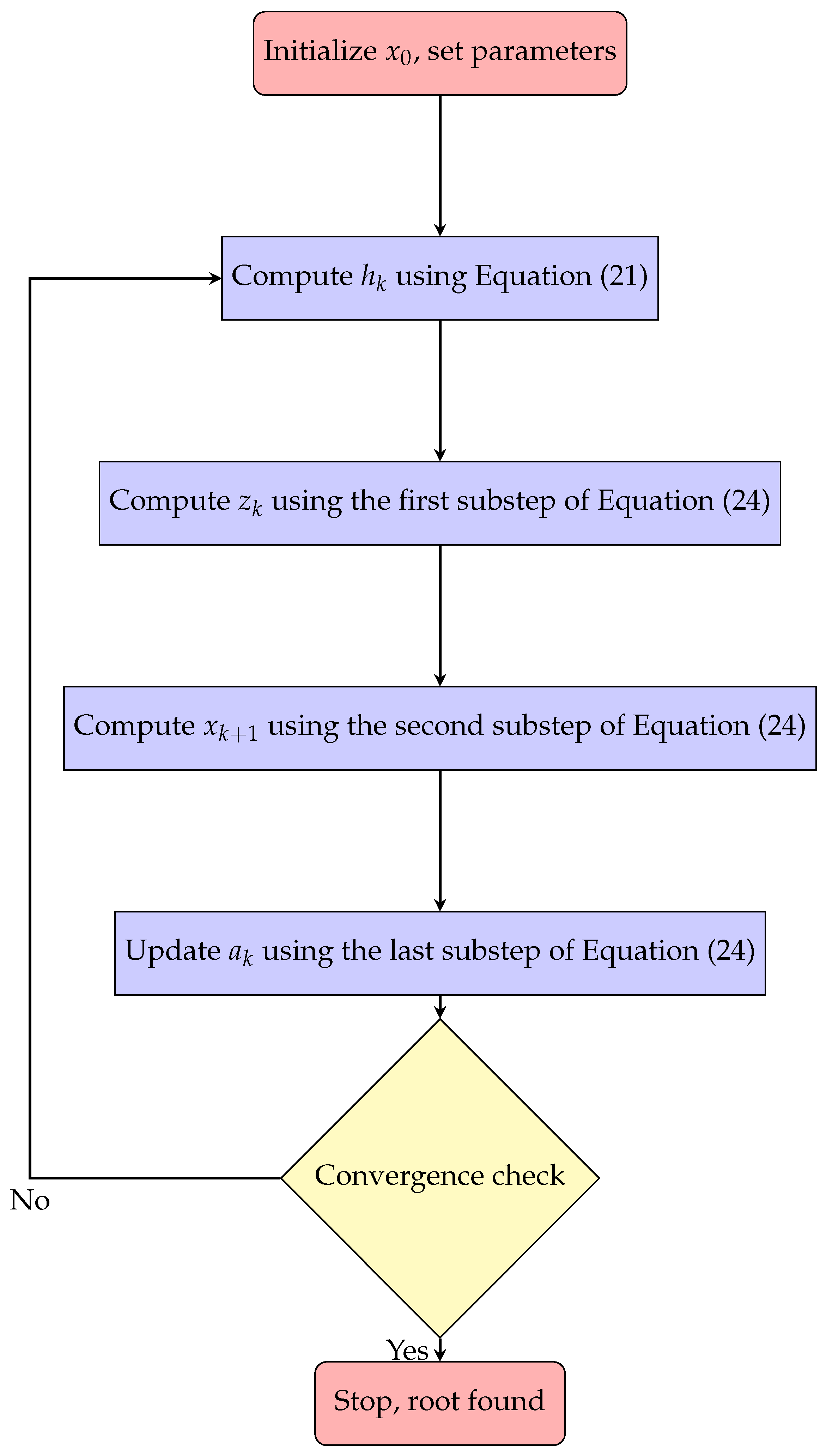
The enhancement of the R-order is attained without introducing any additional functional evaluations, ensuring that the newly developed memory-based method maintains a high TEI. This approach extends the existing scheme (16), effectively increasing the R-order from 4 to $\sqrt{5}+2$. The procedure of the proposed solver is provided in the Flowchart Figure 1.

The proposed acceleration scheme (24) is novel and effective, offering an improvement in the speed, while requiring no further functional evaluations. This advantage sets it apart from optimal two-step methods that lack memory.

Furthermore, it is worth mentioning that another formulation of the presented memory-based scheme can be derived by employing a backward finite difference approximation at the initial stage of the first substep, coupled with a slight modification in the acceleration parameters. In other words, we introduce an alternative memory-based approach (PM2) that preserves the R-order of $r=\sqrt{5}+2$, which is formulated as follows (only $h_k$ differs and Appr will not be changed compared to PM1):

$$\begin{array}{c}\hfill \left\{\begin{array}{c}{h}_k=x_k-\beta f{\left(x_k\right)}^3,\hfill \\ z_k=x_k-{\displaystyle \frac{f\left(x_k\right)}{\mathrm{Appr}}}\left(1+{\displaystyle \frac{a_k}{2}}{\left({\displaystyle \frac{f\left(x_k\right)}{\mathrm{Appr}}}\right)}^2\right),k\ge 0,\hfill \\ x_{k+1}=z_k-{\displaystyle \frac{f\left(z_k\right)}{\mathrm{Appr}}}{\displaystyle \frac{f\left(x_k\right)-1/2f\left(z_k\right)}{f\left(x_k\right)-5/2f\left(z_k\right)}},\hfill \\ a_k=-((1/6)N_3^{‴}\left(x_k\right)/N_3^{\prime }\left(x_k\right)),k\ge 1.\hfill \end{array}\right.\end{array}$$

(33)

Theorem 3.

Consider a function $f\left(x\right)$ that is adequately smooth in the vicinity of its simple zero, denoted by α. If a starting estimate $x_0$ is chosen such that it lies close enough to α, then the solver (33) incorporating memory exhibits an R-order of convergence of no less than 4.23607.

Proof 

Since the proof follows the same reasoning as Theorem 2, it is omitted for brevity. □

From one perspective, since $\beta$ is a parameter that can assume either a positive or negative sign, the order of convergence and the conditions required to achieve it remain identical, as established in Theorems 2 and 3. However, in practical computations, the choice of sign influences the magnitude of posterior error as well as round-off errors, which, in turn, may lead to variations in the final numerical results. These differences will be analyzed in Section 4.

The extension of the proposed techniques to the broader context of solving nonlinear systems of equations $F\left(x\right)=0$ may be systematically achieved by incorporating the formal definition of divided difference operators (DDOs), thereby enabling the effective treatment of these operators in the following manner. Specifically, the first-order DDO of the vector-valued function F, evaluated at the pair of points x and y, can be formulated in a component-wise fashion, described as follows:

$${[x,y;F]}_{i,j}={\displaystyle \frac{F_i(x_1,\dots ,x_j,y_{j+1},\dots ,y_n)-F_i(x_1,\dots ,x_{j-1},y_j,\dots ,y_n)}{x_j-y_j}},1\le i,j\le n.$$

(34)

The expression under consideration represents a bounded linear operator that fulfills the identity $[y,x;F](y-x)=F\left(y\right)-F\left(x\right)$. According to the result established by Potra [31], a necessary and sufficient criterion exists for characterizing the divided difference operator through the framework of the Riemann integral; more specifically, if function F adheres to the Lipschitz-type continuity condition

$$\parallel [x,y;F]-[u,v;F]\parallel \le H(\parallel x-u\parallel +\parallel y-v\parallel ).$$

It is worth mentioning that the work in [32] proposed a symmetric operator for the second-order DDO, albeit at a higher computational expense compared to the first-order DDO. Accordingly, it must be stated that the extension of the proposed solvers for a nonlinear system is inefficient due to the load of computing DDO matrices. Because of this, we restrict our investigation to the scalar case in which the proposed methods are efficient.

4. Computational Aspects

The computational efficacy of various iteration solvers, both with and without memory, could be systematically assessed by employing the definition of the TEI given in Section 1. Based on this criterion, we obtain

$$TEI\left(3\right)\approx 1.4142<TEI\left(4\right)=TEI\left(5\right)\approx 1.4422$$

$$<TEI\left(11\right)=TEI\left(16\right)\approx 1.5874<TEI\left(24\right)=TEI\left(33\right)\approx 1.6180.$$

(35)

We perform an evaluation and comparative analysis of different iterative schemes for determining the simple roots of several nonlinear test functions. These experiments are implemented in the Mathematica programming environment [33], utilizing multiple-precision arithmetic with 5000-digit precision to accurately illustrate the high R-order exhibited by both PM1 and PM2. The comparison is conducted among methods that require the same number of functional evaluations per iterate.

In this section, the computational order of convergence is determined utilizing the following relation [29,34,35]:

$$\zeta ={\displaystyle \frac{ln|\frac{f\left(x_k\right)}{f\left(x_{k-1}\right)}|}{ln|\frac{f\left(x_{k-1}\right)}{f\left(x_{k-2}\right)}|}}.$$

(36)

The obtained $\zeta$ value provides a reliable estimation of the theoretical order of convergence, provided that the iterative method does not exhibit pathological behavior, such as slow convergence in the initial iterations or oscillatory behavior of approximations.

Finally, the pieces of evidence of numerical comparisons for the selected experiments are presented. These experiments were conducted using the stopping criterion set as $\delta ={10}^{-500}$. Additionally, a parameter $\beta =a_0=0.0001$ was used when necessary to fine-tune the iterative process, especially in cases where small initial approximations were employed.

The selection of starting approximations is crucial for the convergence of iteration solvers. A non-iterative method via numerical integration, known as the numerical integration method, was introduced for finding initial approximations [36]. This method uses sigmoid-like functions such as tanh and arctan to approximate the root without requiring derivative information.

Common criteria include checking the difference between successive approximations as follows:

$$|x_k-x_{k-1}|<\tau ,$$

or evaluating the function value at the following approximation:

$$\left|f\right(x_k\left)\right|<\delta .$$

These criteria ensure that the iterative process terminates when the desired accuracy is achieved or when further iterations are unlikely to improve the result.

Example 1.

([37]). We examine the nonlinear test within the domain $D=[1.5,2.5]$ below

$$f_1\left(x\right)=(x^3-8)(x-2tan\left(x\right)),$$

(37)

utilizing an initial estimate of $x_0=1.9$ and $\alpha =2$. The associated observations are provided in

Table 1. Detailed comparative analysis of the results obtained for Example 1.

Solvers	$\mathit{f}\left({\mathit{x}}_1\right)$	$\mathit{f}\left({\mathit{x}}_2\right)$	$\mathit{f}\left({\mathit{x}}_3\right)$	$\mathit{f}\left({\mathit{x}}_4\right)$	$\mathit{f}\left({\mathit{x}}_5\right)$	$\mathit{\zeta }$
NIM	$1.20$	$2.22\times {10}^{-2}$	$7.48\times {10}^{-6}$	$8.46\times {10}^{-13}$	$1.08\times {10}^{-26}$	2.00
OSM	$2.64\times {10}^{-2}$	$2.39\times {10}^{-12}$	$1.60\times {10}^{-52}$	$3.22\times {10}^{-213}$	$5.26\times {10}^{-856}$	4.00
PM1	$5.49\times {10}^{-2}$	$4.22\times {10}^{-11}$	$8.76\times {10}^{-50}$	$1.25\times {10}^{-213}$	$1.09\times {10}^{-907}$	4.23
PM2	$3.33\times {10}^{-2}$	$4.28\times {10}^{-12}$	$5.66\times {10}^{-54}$	$2.21\times {10}^{-231}$	$6.85\times {10}^{-983}$	4.23

.

It is crucial to emphasize that when applying any root-finding algorithm exhibiting local convergence, the careful selection of starting approximations is of paramount significance. If the starting values lie sufficiently near to the desired zeros, the anticipated (analytical) convergence order is observed in practice. Conversely, when the starting approximations are distant from the actual roots, iterative methods tend to exhibit slower convergence, particularly in the early stages of the iterative process.

Example 2.

Next, we analyze the performance of different iterative methods in determining the complex root of the nonlinear problem

$$f_2\left(x\right)=sin\left(x\right)+{\displaystyle \frac{1}{x}}+x+(-1+2I),$$

(38)

by initializing the procedure with $x_0=1.3-2.3I$, where the exact root is given by $\alpha \simeq 0.2886-1.2422I$. The results for this scenario are presented in

Table 2. Detailed comparative analysis of the results obtained for Example 2.

Solvers	$\mathit{f}\left({\mathit{x}}_1\right)$	$\mathit{f}\left({\mathit{x}}_2\right)$	$\mathit{f}\left({\mathit{x}}_3\right)$	$\mathit{f}\left({\mathit{x}}_4\right)$	$\mathit{f}\left({\mathit{x}}_5\right)$	$\mathit{\zeta }$
NIM	$2.13$	$0.93$	$0.04$	$1.20\times {10}^{-4}$	$8.93\times {10}^{-10}$	2.00
OSM	$0.76$	$1.98\times {10}^{-4}$	$1.71\times {10}^{-18}$	$9.53\times {10}^{-75}$	$9.12\times {10}^{-300}$	4.00
PM1	$1.03$	$7.86\times {10}^{-4}$	$8.13\times {10}^{-17}$	$9.95\times {10}^{-72}$	$2.30\times {10}^{-304}$	4.23
PM2	$0.95$	$5.63\times {10}^{-4}$	$2.02\times {10}^{-17}$	$2.72\times {10}^{-74}$	$3.23\times {10}^{-315}$	4.23

.

A close inspection of Table 1 and Table 2 clearly demonstrates that the root approximations exhibit remarkable accuracy when the proposed memory-based method is employed. Furthermore, the values from the fourth and fifth iterations, as reported in Table 1 and Table 2, are included solely to illustrate the convergence speed of the evaluated solvers. In most practical applications, such additional iterations are generally unnecessary.

The numerical observations presented in Table 1 and Table 2 illustrate the convergence behavior of various iterative methods applied to solve nonlinear scalar equations. In Example 1, the methods were tested on the function $f_1\left(x\right)$ within the domain $D=[1.5,2.5]$, with a starting guess $x_0=1.9$. The obtained results demonstrate that the OSM, the PM1, and the PM2 exhibit significantly faster convergence rates compared to the NIM. Specifically, OSM, PM1, and PM2 attain highly accurate solutions within just five iterations, with residual function values decreasing to approximately ${10}^{-856}$, ${10}^{-907}$, and ${10}^{-983}$, respectively. Additionally, the convergence factor $\zeta$ confirms the expected order of convergence, where NIM converges quadratically ($\zeta =2.00$), while OSM, PM1, and PM2 attain higher convergence rates. The higher accuracy of PM1 and PM2 compared to OSM suggests the effectiveness of approximations in accelerating convergence.

For the complex-valued nonlinear Equation $f_2\left(x\right)$ analyzed in Example 2, a similar pattern emerges. The iterative methods were initialized at $x_0=1.3-2.3I$, targeting the exact complex root $\alpha \simeq 0.2886-1.2422I$. The numerical findings in Table 2 further confirm the superiority of higher-order methods over NIM. OSM, PM1, and PM2 exhibit remarkably small residual function values in just five iterations, dropping to approximately ${10}^{-300}$, ${10}^{-304}$, and ${10}^{-315}$, respectively. 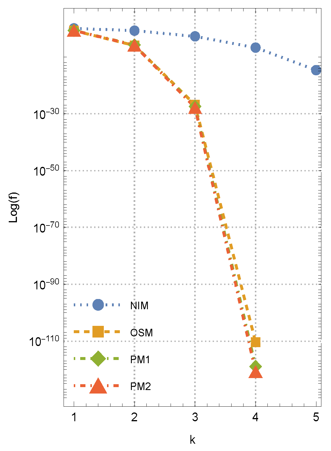Again, the order of convergence values, $\zeta \approx 4.00$ for OSM and $\zeta \approx 4.23$ for PM1 and PM2, validate the high efficiency of these methods. Notably, while NIM requires more iterations to reach a reasonable accuracy, the new approaches maintain their superior convergence behavior, reinforcing their practical utility in solving nonlinear problems with complex roots. For Example 2, we provide Figure 2, which shows the history of convergence for another initial approximation through the comparison of different methods.

A value for parameter beta has been selected for numerical testing and it is better to choose a small value in order to lead to larger attraction basins. However, based on the structure of either PM1 or PM2, memorization has been done only on $a_k$, which means that there is no adaptation or acceleration based on $\beta$. This is because in $h_k=x_k-\beta f{\left(x_k\right)}^3$, there is a power of three for $f\left(x_k\right)$.

Moreover, the developed memory-based approaches (24) and (33) have been applied to a range of test problems, consistently yielding results that align with the aforementioned observations. Consequently, we can assert that the theoretical findings are well supported by numerical tests, thereby affirming the robustness and high computational efficiency of the proposed method.

5. Conclusions

Classical iteration solvers, such as Newton’s scheme, are widely employed due to their quadratic convergence properties; however, their efficiency can be further enhanced by incorporating memory, which exploits previously computed information to accelerate convergence without increasing the number of function evaluations. In this article, we have introduced a scheme with memory. The construction of this method leverages the existing framework of Newton’s method while incorporating memory to improve the convergence properties. Theoretical analysis confirms that the presented scheme achieves a higher R-order of convergence compared to the original two-point solver, without increasing the computational cost in terms of functional evaluations. Numerical experiments further validate the efficiency and robustness of the method, demonstrating its superiority in terms of convergence speed and accuracy.

The success of the proposed solver with memory provides some avenues for future works. Firstly, the extension of this approach to other families of iteration solvers, such as Halley’s or Chebyshev’s schemes, could be explored to further enhance their convergence properties. Secondly, the application of the method with memory to systems of nonlinear equations is a promising direction. Additionally, the development of hybrid methods that combine memory-based techniques with other acceleration strategies, such as weight functions or parameter optimization, could lead to even more efficient algorithms.