Superconvergence of Mixed Finite Element Method with Bernstein Polynomials for Stokes Problem

Abstract

In this paper, we employ interpolation and projection methodologies to establish a superconvergence outcome for the Stokes problem, as approximated by the mixed finite element method (FEM) utilizing Bernstein polynomial basis functions. It is widely recognized that the convergence rate of the FEM in the L²-norm is $\mathcal{O}\left(h^{m+2}\right)$. However, this paper presents an innovative superconvergence result: specifically, in terms of the L²-norm, the error convergence rate between the mixed finite element approximate solution and the local projection is $\mathcal{O}\left(h^{m+2}\right)$, with m denoting the order of the Bernstein polynomial basis function.

1. Introduction

With the development of engineering mechanics and computers, FEM [1,2,3] has become an important tool to solve partial differential equations (PDEs) [4,5,6], and the accuracy requirement of finite element numerical solutions is also increasing. So, how to further improve the accuracy of finite element solutions has become an increasingly significant research topic. The following are some commonly used methods, including increasing the number of calculation iterations, selecting an appropriate mesh size, determining suitable basis functions, and using the superconvergence of finite element solutions. Additionally, the meshless method [7,8] has been proposed as an effective approach to mitigate issues related to meshing. Now, the superconvergence of finite element solutions has become an important study area [9,10,11]. Superconvergence is the use of simple post-processing techniques such as interpolation and weighted averaging to significantly improve the approximation accuracy of finite element solutions without increasing the amount of calculation. In this paper, our main purpose is to verify the superconvergence result of a Stokes problem by using an interpolation method.

Superconvergence analysis offers significant advantages in enhancing computational accuracy, streamlining the calculation process, and bolstering flexibility and adaptability, providing it important application value for solving a wide range of complex problems. In practical application, the study of superconvergence can help us to improve the accuracy of finite element solutions, thereby more accurately simulating the behavior of complex systems, which has important research value in Structural Mechanics [12,13], Telecommunication Technology [14,15,16], Physics [17,18], and other fields [19,20,21].

Since the 1970s, many experts have conducted extensive research on the phenomenon of superconvergence analysis [22,23,24,25]. In 1973, Douglas and Dupont [26] proved the superconvergence of finite element solutions of two-point boundary value problems by local projection. In 1985, Douglas and Robert [27] proved the superconvergence of linear elliptic boundary value problems by using the kernel average method. In 1999, Ewing et al. [28] established the superconvergence results of approximate solutions of second-order elliptic equations by using the mixed FEM on quadrilateral elements. In 2002, Ewing et al. [29] obtained the superconvergence of numerical solutions of elliptic problems by using a Raviart–Thomas mixed FEM on rectangular elements. In 2009, Chen and Dai [30] proved the superconvergence of the optimal control problem for semilinear elliptic equations. In 2012, Shi et al. [31] used interpolation post-processing technology to derive the convergence and superconvergence results of a Signorini problem. In 2024, Shi and Zhang [32] obtained superconvergence results of nonlinear parabolic integro-differential equations via interpolation post-processing technology.

The Bernstein polynomial basis function was put forward by Sergei Natanovich Bernstein [33] in 1912, which was used to study the properties of piecewise curves. In recent years, the research on Bernstein polynomials has achieved remarkable progress, and many scholars have strongly promoted it. For example, the introduction of new forms such as the $\lambda$-Bernstein polynomial and $\alpha$-Bernstein polynomial not only enriches the theoretical framework of the Bernstein polynomial but also greatly expands its application scope in practical problems.

In 2010, Ye et al. [34] proposed a set of new Bézier basis functions with shape parameter $\lambda$, which provided a flexible framework for curve and surface modeling. In 2018, Cai et al. [35] popularized the Bernstein operator, which enhanced the flexibility of the $\lambda$-Bézier basis function in approximation problems and provided better tools for various approximation tasks. In the same year, Hu et al. [36] constructed a generalized developable Bézier surface whose shape parameters can be adjusted and realized various geometric configurations, which further verified the practical application value of the $\lambda$-Bézier basis function. In the field of approximation theory, in 1965, Schurer [37] introduced a non-negative integer into the classical Bernstein basis and put forward the Schurer operator, which laid the foundation for subsequent research. In 2018, Yilmaz et al. [38] introduced the generalized Baskakov–Schurer–Szász operator, which significantly improved the approximation performance by retaining the exponential function characteristics. In 2023, Ayman-Mursaleen et al. [39] incorporated the shape parameter $\alpha$ into the Bernstein–Schurer operator, which further improved its uniform approximation ability. In this paper, our objective is to establish the superconvergence results of finite element solutions for Stokes equations by utilizing interpolation and post-processing techniques with Bernstein tensor product polynomials on rectangular domains.

This paper is organized as follows. In Section 2, we review the content of the Stokes equation and mixed FEM. In Section 3, we establish a basic framework of superconvergence analysis. In Section 4, we demonstrate some superconvergence results for mixed finite elements. In Section 5, we use a numerical example to verify the correctness and feasibility of the theory. In Section 6, we formulate the conclusion and consider prospects for future work.

2. Review the Stokes Problem and Mixed FEM

Now we consider the Stokes equation with homogeneous Dirichlet boundary conditions. Let $\Omega$ be an open bounded set on ${\mathbb{R}}^d(d=2,3)$ with Lipschitz continuous boundary.

$$\begin{array}{c}\hfill \left\{\begin{array}{cc}\hfill -\nabla ·\mathbb{T}(\mathbf{u},p)& =\mathbf{f},in\Omega ,\hfill \\ \hfill \nabla ·\mathbf{u}& =0,in\Omega ,\hfill \\ \hfill \mathbf{u}& =\mathbf{0},in\partial \Omega ,\hfill \end{array}\right.\end{array}$$

(1)

where $\mathbf{f}\in L^2{(\Omega )}^d$ represents the unit external volumetric force acting on the fluid, $\mathbf{u}\in H^1{(\Omega )}^d$ is the velocity vector, $p\in L^2(\Omega )$ refers to fluid pressure, $\mathbb{T}(\mathbf{u},p)=2\nu \mathbb{D}\left(u\right)-p\mathbb{I}$ is stress tensor, and $\nu >0$ is a given constant representing the viscosity coefficient of the fluid; in more detail, the symmetric velocity gradient can be written as

$$\mathbb{D}\left(\mathbf{u}\right)=\left(\begin{array}{cc}{\displaystyle \frac{\partial u_1}{\partial x}}& {\displaystyle \frac{1}{2}}\left({\displaystyle \frac{\partial u_1}{\partial y}}+{\displaystyle \frac{\partial u_2}{\partial x}}\right)\\ {\displaystyle \frac{1}{2}}\left({\displaystyle \frac{\partial u_1}{\partial y}}+{\displaystyle \frac{\partial u_2}{\partial x}}\right)& {\displaystyle \frac{\partial u_2}{\partial y}}\end{array}\right).$$

(2)

In this paper, we assume $d=2,\nu =1$. We set $\nu =1$ merely for the convenience of the proof, which does not affect the generality and validity of the final results.

Define a Sobolev space as follows $\mathbf{U}=H^1(\Omega )\times H^1(\Omega )$ with the norm

$${\parallel \mathbf{u}\parallel }_{\mathbf{U}}={\left({\parallel \mathbf{u}\parallel }_0^2+{\parallel \nabla ·\mathbf{u}\parallel }_0^2\right)}^{{\displaystyle \frac{1}{2}}}.$$

(3)

Let $W=L_0^2(\Omega )$ be the space of functions in $L^2(\Omega )$ with mean value zero.

The variational form of Equation (1) finds $(\mathbf{u};p)\in {\left(H^1\right)}^2\times W$, satisfying

$$\begin{array}{cc}\hfill a(\mathbf{u},\mathbf{v})-b(\mathbf{v},p)& =(\mathbf{f},\mathbf{v}),\forall \mathbf{v}\in {\left(H_0^1\right)}^2,\hfill \\ \hfill b(\mathbf{u},q)& =0,\forall q\in W,\hfill \end{array}$$

(4)

where

$$\begin{array}{cc}\hfill a(\mathbf{u},\mathbf{v})& ={\int }_{\Omega }2\mathbb{D}\left(\mathbf{u}\right):\mathbb{D}\left(\mathbf{v}\right)dxdy,\hfill \\ \hfill b(\mathbf{u},q)& =(\nabla ·\mathbf{u},q)={\int }_{\Omega }\nabla ·\mathbf{u}qdxdy,\hfill \end{array}$$

(5)

here,

$$\begin{array}{cc}\hfill & \mathbb{D}\left(\mathbf{u}\right):\mathbb{D}\left(\mathbf{v}\right)\hfill \\ \hfill =& \begin{array}{c}\hfill {\displaystyle \frac{\partial u_1}{\partial x}}{\displaystyle \frac{\partial v_1}{\partial x}}+{\displaystyle \frac{\partial u_2}{\partial y}}{\displaystyle \frac{\partial v_2}{\partial y}}+{\displaystyle \frac{1}{2}}{\displaystyle \frac{\partial u_1}{\partial y}}{\displaystyle \frac{\partial v_1}{\partial y}}\end{array}+{\displaystyle \frac{1}{2}}{\displaystyle \frac{\partial u_1}{\partial y}}{\displaystyle \frac{\partial v_2}{\partial x}}+{\displaystyle \frac{1}{2}}{\displaystyle \frac{\partial u_2}{\partial x}}{\displaystyle \frac{\partial v_1}{\partial y}}+{\displaystyle \frac{1}{2}}{\displaystyle \frac{\partial u_2}{\partial x}}{\displaystyle \frac{\partial v_2}{\partial x}}.\hfill \end{array}$$

(6)

and fulfills the following continuity conditions on page 57 of [40]

$$\begin{array}{cc}\hfill a\left(\mathbf{u},\mathbf{v}\right)& \le {∥\mathbf{u}∥}_{\mathbf{U}}{∥\mathbf{v}∥}_{\mathbf{U}},\forall \mathbf{u},\mathbf{v}\in \mathbf{U},\hfill \\ \hfill b(\mathbf{v},q)& \le {∥\mathbf{v}∥}_{\mathbf{U}}{∥q∥}_0,\forall \mathbf{v}\in \mathbf{U},\forall q\in W.\hfill \end{array}$$

(7)

Let ${\mathbf{U}}_h\subset \mathbf{U}$ and $W_h\subset W$ be any two finite element spaces for velocity $\mathbf{u}$ and pressure p, respectively. In order to generate a locally finite-dimensional space ${\mathbf{U}}_h$ and $W_h$, we first introduce the one-dimensional Bernstein polynomial basis functions.

Definition 1.

Bernstein polynomial basis of degree n is defined by

$$B_i^n\left(x\right)=\left({\displaystyle \genfrac{}{}{0pt}{}{n}{i}}\right)x^i{(1-x)}^{n-i},i=1,2,\dots ,n,$$

(8)

where $\left({\displaystyle \genfrac{}{}{0pt}{}{n}{i}}\right)={\displaystyle \frac{n!}{i!(n-i)!}},i=0,1,\dots ,n.$ For simplicity, when $i<0$ or $i>n$, let $B_i^n\left(x\right)=0$, $x\in [0,1]$.

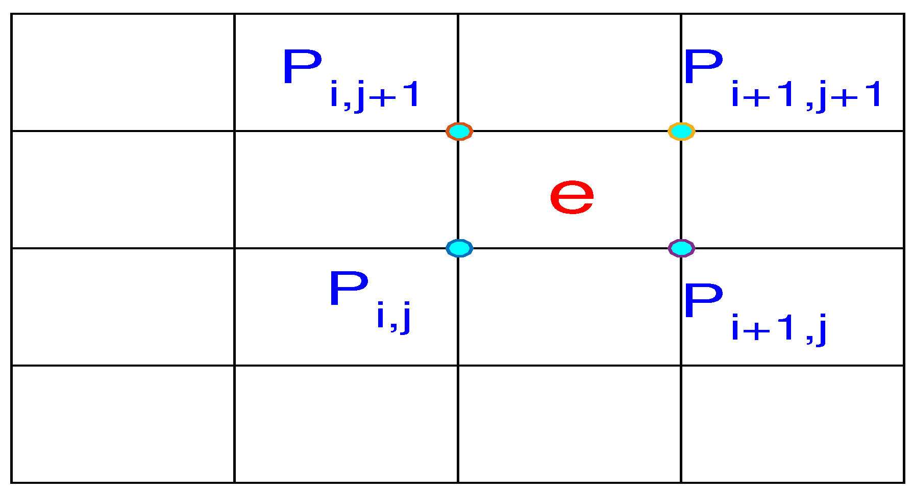
Then, we divide the bounded region $\Omega$ into finite uniform rectangles e and remember the division as ${\mathcal{T}}_h=\left\{e\right\}$. Later, in order to construct the shape function on the local element, we take any element e on ${\mathcal{T}}_h$ and set its vertexes as $P_{i,j}(x_i,y_j),P_{i+1,j}(x_{i+1},y_j),P_{i,j+1}(x_i,y_{j+1}),$$P_{i+1,j+1}(x_{i+1},y_{j+1})$, as shown in Figure 1.

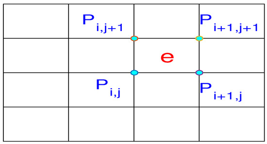
Figure 1. Element mesh on subdivision ${\mathcal{T}}_h$.

In this paper, we choose $m\times n$ tensor product Bernstein polynomial function ${\mathcal{B}}_{i,j}^{m,n}$ as basis function for the finite element space; here, m and n are both positive integers. Bernstein polynomial basis functions of tensor-product type are generated from Equation (8) by making a tensor.

Definition 2.

A tensor-product-type Bernstein polynomial basis of $m\times n$ degree is in the reference element $[0,1]\times [0,1]$ defined by

$${\mathcal{B}}_{i,j}^{m,n}(s,\tau )=B_i^m\left(s\right)B_j^n\left(\tau \right),i=0,1,\dots ,m,j=0,1,\dots ,n.$$

(9)

Let $\overline{s}=(\mathbf{b}-\mathbf{a})s+\mathbf{a},\overline{\tau }=(\mathbf{d}-\mathbf{c})\tau +\mathbf{c}$, where $\overline{s}\in [\mathbf{a},\mathbf{b}],\overline{\tau }\in [\mathbf{c},\mathbf{d}]$ and where $[\mathbf{a},\mathbf{b}]$ and $[\mathbf{c},\mathbf{d}]$, respectively, refer to any closed interval. We obtain the Bernstein polynomial basis function of tensor product type on any element

$${\overline{\mathcal{B}}}_{i,j}^{m,n}(\overline{s},\overline{\tau })=B_i^m\left({\displaystyle \frac{\overline{s}-\mathbf{a}}{\mathbf{b}-\mathbf{a}}}\right)B_j^n\left({\displaystyle \frac{\overline{\tau }-\mathbf{c}}{\mathbf{d}-\mathbf{c}}}\right),i=0,1,\dots ,m,j=0,1,\dots ,n.$$

(10)

Subsequently, complete affine transformation; let $s={\displaystyle \frac{x-x_i}{h_1}}$, $\tau ={\displaystyle \frac{y-y_j}{h_2}}$, where $h_1$ and $h_2$ refer to the grid size in the x direction and the y direction respectively. So, we obtain the shape function on the local element e

$$\begin{array}{c}\hfill {\mathcal{B}}_{i,j}^{m,n}(x,y)=B_i^m\left({\displaystyle \frac{x-x_i}{h_1}}\right)B_j^n\left({\displaystyle \frac{y-y_j}{h_2}}\right),i=0,1,\dots ,m,j=0,1,\dots ,n.\end{array}$$

(11)

It should be noted that, in order to satisfy the inf-sup condition on page 342 of [40], the polynomial degree in $W_h$ must be at least one order lower than that in ${\mathbf{U}}_h$. Assume that the polynomial space ${\mathbf{U}}_h$ consists of $P_k$ for $k\ge 2$, which contains polynomials of degree no more than k, and $W_h$ is composed of $P_{k-1}$.

From Equation (11), the following finite-dimensional space can be obtained:

$$\begin{array}{cc}\hfill & {\mathbf{U}}_h=\{\mathbf{u}\in \mathbf{U},\mathbf{u}{|}_e\in span\{\left\{{\mathcal{B}}_{i,j}^{m,m}\right\}\times \left\{{\mathcal{B}}_{i,j}^{m,m}\right\}\},e\in {\mathcal{T}}_h\},\hfill \\ & W_h=\{w\in W,w{|}_e\in span\left\{{\mathcal{B}}_{i,j}^{m-1,m-1}\right\},e\in {\mathcal{T}}_h\}.\hfill \end{array}$$

(12)

where e is any rectangle element in ${\mathcal{T}}_h$; h and l represent the degree of x and y in $W_h$, respectively. Define ${\mathbf{U}}_{h0}=\{\mathbf{u}\in {\mathbf{U}}_h,\mathbf{u}=\mathbf{0}on\partial \Omega \}$.

Then, the discrete scheme of Equation (4) is provided by ${\mathbf{u}}_h\in {\mathbf{U}}_h$ and $p_h\in W_h$, satisfying

$$\begin{array}{cc}\hfill a({\mathbf{u}}_h,\mathbf{v})-b(\mathbf{v},p_h)& =(\mathbf{f},\mathbf{v}),\forall \mathbf{v}\in {\mathbf{U}}_{h0},\hfill \\ \hfill b({\mathbf{u}}_h,q)& =0,\forall q\in W_h.\hfill \end{array}$$

(13)

It is known that Equation (13) satisfies the inf-sup condition, which can be verified by using a projection operator ${\pi }_h:\mathbf{U}\to {\mathbf{U}}_h$ that satisfies

$$(\nabla ·(\mathbf{u}-{\pi }_h\mathbf{u}),q)=0,\forall q\in W_h.$$

(14)

For any sufficiently smooth vector-valued function $\mathbf{u}\in \mathbf{U}$, $e\in {\mathcal{T}}_h$, we define its local projection ${\pi }_e\mathbf{u}\in {\mathbf{U}}_h$, which satisfies the following equations:

$$\begin{array}{cc}\hfill & {\int }_{{\mathsf{\ell }}_i}(\mathbf{u}-{\pi }_e\mathbf{u})·{\mathbf{n}}_i\varphi ds=0,\varphi \in P_{m-2}\left({\mathsf{\ell }}_i\right),i=1,2,3,4,\hfill \\ \hfill & {\int }_e(\mathbf{u}-{\pi }_e\mathbf{u})·\mathit{\psi }dxdy=0,\mathit{\psi }\in {\mathcal{B}}_{i,j}^{m-2,m-2}\times {\mathcal{B}}_{i,j}^{m-2,m-2},\hfill \end{array}$$

(15)

where ${\mathsf{\ell }}_i,(i=1,2,3,4)$ represents the edges of the element e.

Next, we use local projection operator ${\pi }_e$ to define global projection operator ${\pi }_h:\mathbf{U}\to {\mathbf{U}}_h$

$$\left({\pi }_h\mathbf{u}\right)(x,y)={\pi }_e\mathbf{u}(x,y)\forall (x,y)\in e,e\in {\mathcal{T}}_h,$$

(16)

which satisfies Formula (14). Furthermore, ${\pi }_h$ can be written in the form of two components as follows:

$${\pi }_h\mathbf{u}=({\pi }_1{u}_1,{\pi }_2{u}_2),$$

(17)

among them, ${\pi }_1$ and ${\pi }_2$ are independent of each other.

Lastly, define the $L^2$ projection ${\mathcal{P}}_h:W\to W_h$.

3. A General Framework for Superconvergence

In order to prove superconvergence analysis, we first provide a theorem to describe the error estimation between projection and approximate solution.

Theorem 1.

Assume $(\mathbf{u};p)\in {\left(H^1\right)}^2\times L_0^2$ is the solution of Equation $\left(4\right)$. Let $({\mathbf{u}}_h;p_h)\in {\mathbf{U}}_h\times W_h$ solve Equation $\left(13\right)$. Let

$${\mathbf{e}}_h={\mathbf{u}}_h-{\pi }_h\mathbf{u};{\xi }_h=p_h-{\mathcal{P}}_{h}p.$$

(18)

If there exists a constant $M=M(\mathbf{u},p)$ and parameter s satisfying

$$\underset{\mathbf{v}\in {\mathbf{U}}_{h0}}{sup}{\displaystyle \frac{a((\mathbf{u}-{\pi }_h\mathbf{u}),\mathbf{v})}{{\parallel \mathbf{v}\parallel }_{\mathbf{U}}}}\le M(\mathbf{u},p)h^{m+s},$$

(19)

then there will be a constant C that is independent of h such that

$$\parallel {\mathbf{e}}_h{\parallel }_0+{\parallel {\xi }_h\parallel }_0\le CM(\mathbf{u},p)h^{m+s}.$$

(20)

Proof. 

Subtract Equation (13) from Equation (4) and we obtain the error equation

$$\begin{array}{cc}\hfill a(\mathbf{u}-{\mathbf{u}}_h,\mathbf{v})-b(\mathbf{v},p-p_h)& =0,\forall \mathbf{v}\in {\mathbf{U}}_{h0},\hfill \\ \hfill b(\mathbf{u}-{\mathbf{u}}_h,q)& =0,\forall q\in W_h.\hfill \end{array}$$

(21)

So, we have

$$\begin{array}{cc}\hfill a({\mathbf{u}}_h-{\pi }_h\mathbf{u},\mathbf{v})-b(\mathbf{v},p_h-{\mathcal{P}}_{h}p)& =a(\mathbf{u}-{\pi }_h\mathbf{u},\mathbf{v})-b(\mathbf{v},p-{\mathcal{P}}_{h}p),\forall \mathbf{v}\in {\mathbf{U}}_{h0},\hfill \\ \hfill b(\mathbf{u}-{\pi }_h\mathbf{u},q)+b({\pi }_h\mathbf{u}-{\mathbf{u}}_h,q)& =0,\forall q\in W_h.\hfill \end{array}$$

(22)

Based on the definition of $L^2$ projection and Equation (14), substituting Equation (18) into the above equation yields

$$\begin{array}{ccc}\hfill a({\mathbf{e}}_h,\mathbf{v})-b(\mathbf{v},{\xi }_h)& =a(\mathbf{u}-{\pi }_h\mathbf{u},\mathbf{v}),\hfill & \hfill \forall \mathbf{v}\in {\mathbf{U}}_{h0},\\ \hfill b({\mathbf{e}}_h,q)& =0,\hfill & \hfill \forall q\in W_h.\end{array}$$

(23)

From the second equation of Equation (23), we find that $\nabla ·{\mathbf{e}}_h=0$. In the first equation of Equation (23), by taking $\mathbf{v}={\mathbf{e}}_h$, and, in the second equation, taking $q={\xi }_h$, then we have

$$a({\mathbf{e}}_h,{\mathbf{e}}_h)=a(\mathbf{u}-{\pi }_h\mathbf{u},{\mathbf{e}}_h).$$

(24)

From condition (19) and $\nabla ·{\mathbf{e}}_h=0$, it can be inferred that

$$a({\mathbf{e}}_h,{\mathbf{e}}_h)\le CM(\mathbf{u},p)h^{m+s}{\parallel {\mathbf{e}}_h\parallel }_0,$$

(25)

so,

$$\parallel {\mathbf{e}}_h{\parallel }_0\le C{h}^{m+s}M(\mathbf{u},p).$$

(26)

Then, now we estimate the $L^2$-norm of ${\xi }_h$. From the inf-sup condition and continuity condition, we arrive at

$$\begin{array}{cc}\hfill \parallel {\xi }_h{\parallel }_0& \le C\underset{\mathbf{v}\in {\mathbf{U}}_{h0}}{sup}{\displaystyle \frac{b(\mathbf{v},{\xi }_h)}{{\parallel \mathbf{v}\parallel }_{\mathrm{U}}}}\hfill \\ \hfill & =C\underset{\mathbf{v}\in {\mathbf{U}}_{h0}}{sup}{\displaystyle \frac{b(\mathbf{v},p_h-p)}{{\parallel \mathbf{v}\parallel }_{\mathrm{U}}}}\hfill \\ \hfill & =C\underset{\mathbf{v}\in {\mathbf{U}}_{h0}}{sup}{\displaystyle \frac{a(\mathbf{v},{\mathbf{u}}_h-\mathbf{u})}{{\parallel \mathbf{v}\parallel }_{\mathbf{U}}}}\hfill \\ \hfill & =C\underset{\mathbf{v}\in {\mathbf{U}}_{h0}}{sup}{\displaystyle \frac{a(\mathbf{v},{\mathbf{u}}_h-{\pi }_h\mathbf{u})+a(\mathbf{v},{\pi }_h\mathbf{u}-\mathbf{u})}{{\parallel \mathbf{v}\parallel }_{\mathbf{U}}}}\hfill \\ \hfill & \le C\underset{\mathbf{v}\in {\mathbf{U}}_{h0}}{sup}{\displaystyle \frac{a(\mathbf{v},\mathbf{u}-{\pi }_h\mathbf{u})}{{\parallel \mathbf{v}\parallel }_{\mathbf{U}}}}+C{\parallel {\mathbf{u}}_h-{\pi }_h\mathbf{u}\parallel }_0\hfill \\ \hfill & \le C{h}^{m+s}M(\mathbf{u},p).\hfill \end{array}$$

(27)

This completes the proof. □

4. Main Results of Superconvergence

Theorem 1 shows that, if a corresponding estimate in bilinear form $\mathcal{A}\left(\mathbf{v}\right)=a((\mathbf{u}-{\pi }_h\mathbf{u}),\mathbf{v})$ is established in a mixed finite element space ${\mathbf{U}}_{h0}$, superconvergence will be guaranteed. In this section, we divide $\mathcal{A}\left(\mathbf{v}\right)$ into six parts and verify error estimates separately, ultimately achieving the desired superconvergence result.

Let us introduce some short-hand notation for partial derivatives, the multi-index notation. A multi-index, $\alpha$, is an n-tuple of non-negative integers, ${\alpha }_i$. The length of $\alpha$ is provided by

$$|\alpha |:=\sum _{i=1}^n{\alpha }_i.$$

(28)

For $\varphi \in {\mathbb{C}}^{\infty }$, denote by

$$D^{\alpha }\varphi ={\left({\displaystyle \frac{\partial }{\partial x_1}}\right)}^{{\alpha }_1}\dots {\left({\displaystyle \frac{\partial }{\partial x_n}}\right)}^{{\alpha }_n}\varphi .$$

(29)

First, let us review the definition of the norm in Sobolev spaces. Denote the seminorm and the norm in the Sobolev space $W^{k,r}(\Omega )$ with integer $k\ge 0$ and real number $r\ge 1$ by

$${|\mathbf{u}|}_{k,r;\Omega }=\sum _{|\alpha |=k}\parallel D^{\alpha }{\mathbf{u}\parallel }_{L^r}{,\parallel \mathbf{u}\parallel }_{k,r;\Omega }=\sum _{j=0}^k{|\mathbf{u}|}_{j,r;\Omega }.$$

And, define the seminorm of any piecewise polynomial q with

$${|q|}_{k,r,h}=\sum _{|\alpha |=k}{\left(\sum _{e\in T_h}{\parallel D^{\alpha }q\parallel }_{L^r\left(e\right)}^r\right)}^{1/r}.$$

Let $\sigma$ be any smooth vector-valued function on a rectangular element e and satisfy the following system:

$$\begin{array}{ccc}\hfill {\int }_{{\mathsf{\ell }}_i}\sigma dy& =0,\hfill & \hfill i=1,2,3,4,\\ \hfill {\int }_e{x}^j\sigma dxdy& =0,\hfill & \hfill 0\le j\le \lambda -1.\end{array}$$

(30)

We introduce $\sigma$ to facilitate the estimation of the following components. Therefore, the following lemma holds.

Lemma 1

([29]). Let ${\mathsf{\ell }}_1,{\mathsf{\ell }}_3$ be two vertical sides of element $e=[x_i,x_{i+1}]\times [y_j,y_{j+1}]$, $2h_e=x_{i+1}-x_i$ is the length of ${\mathsf{\ell }}_2$, and ${\mathsf{\ell }}_4$, $(x_e,y_e)$ is the center of e, $E\left(x\right)={(x-x_e)}^2-h_e^2$. Then, for any integer $k\le \lambda +1$, we have

$${\int }_e{(x-x_e)}^k\sigma dxdy={\displaystyle \frac{{(-1)}^{k}k!}{(2k+2)!}}{\int }_e{E}^{k+1}\left(x\right){\partial }_x^{k+2}\sigma dxdy.$$

(31)

For the bilinear form $\mathcal{A}\left(\mathbf{v}\right)=a((\mathbf{u}-{\pi }_h\mathbf{u}),\mathbf{v})$, where $\mathbf{v}=(v_1,v_2)$, we can write the bilinear form $\mathcal{A}\left(\mathbf{v}\right)$ as six components

$$\begin{array}{cc}\hfill \mathcal{A}\left(\mathbf{v}\right)& =\left[2({\partial }_x(u_1-{\pi }_1{u}_1),{\partial }_x{v}_1)+({\partial }_y(u_1-{\pi }_1{u}_1),{\partial }_y{v}_1)\right]+[2({\partial }_y(u_2-{\pi }_2{u}_2),{\partial }_y{v}_2)\hfill \\ \hfill & +({\partial }_x(u_2-{\pi }_2{u}_2),{\partial }_x{v}_2)]+({\partial }_x(u_2-{\pi }_2{u}_2),{\partial }_y{v}_1)+({\partial }_y(u_1-{\pi }_1{u}_1),{\partial }_x{v}_2)\hfill \\ \hfill & =\sum _{e\in {\mathcal{T}}_h}{\left(2({\partial }_x(u_1-{\pi }_1{u}_1),{\partial }_x{v}_1)\right)}_e+\sum _{e\in {\mathcal{T}}_h}{\left(({\partial }_y(u_1-{\pi }_1{u}_1),{\partial }_y{v}_1)\right)}_e\hfill \\ & +\sum _{e\in {\mathcal{T}}_h}{\left(2({\partial }_y(u_2-{\pi }_2{u}_2),{\partial }_y{v}_2)\right)}_e+\sum _{e\in {\mathcal{T}}_h}{\left(({\partial }_x(u_2-{\pi }_2{u}_2),{\partial }_x{v}_2)\right)}_e\hfill \\ \hfill & +\sum _{e\in {\mathcal{T}}_h}{({\partial }_x(u_2-{\pi }_2{u}_2),{\partial }_y{v}_1)}_e+\sum _{e\in {\mathcal{T}}_h}{({\partial }_y(u_1-{\pi }_1{u}_1),{\partial }_x{v}_2)}_e\hfill \\ \hfill & ={\mathcal{A}}_1+{\mathcal{A}}_2+{\mathcal{A}}_3+{\mathcal{A}}_4+{\mathcal{A}}_5+{\mathcal{A}}_6.\hfill \end{array}$$

(32)

Next, we will begin to estimate the six components of the bilinear form.

Lemma 2.

For any integer $m\ge 1$ and a sufficiently smooth function $u_1$ on the rectangular element e, let $v_1$ be a polynomial with degree of x and y no more than m and $v_2$ be any sufficiently smooth function on e. Then, there will be an area integral $J_{1,e}$ on e, and $J_{1,e}$ satisfies

$$\begin{array}{cc}\hfill & {\left(2({\partial }_x(u_1-{\pi }_1{u}_1),{\partial }_x{v}_1)\right)}_e\hfill \\ & =J_{1,e}-{\displaystyle \frac{{(-1)}^m}{\left(2m\right)!}}({\int }_{{\mathsf{\ell }}_2}-{\int }_{{\mathsf{\ell }}_4})F^m\left(y\right){\partial }_x{\partial }_y^{m+1}{u}_1{\partial }_y^{m-1}{v}_1(x,y_e)dy,\hfill \end{array}$$

(33)

and follows the estimate

$$\begin{array}{cc}\hfill |J_{1,e}|& \le {\displaystyle \frac{2{(-1)}^m{k}_e^{2m}}{\left(2m\right)!}}[|u_1{|}_{m+3,\alpha ;e}|v_1{|}_{m-1,\beta ;e}+k_e|u_1{|}_{m+3,\alpha ;e}{|v_1|}_{2,\beta ;e}\hfill \\ \hfill & +{\displaystyle \frac{k_e^2}{(2m+1)(2m+2)}}|u_1{|}_{m+3,\alpha ;e}{|v_1|}_{2,\beta ;e}],\hfill \end{array}$$

(34)

where α and β are a pair of conjugate numbers and satisfy ${\displaystyle \frac{1}{\alpha }}+{\displaystyle \frac{1}{\beta }}=1,\alpha ,\beta \ge 1$.

Proof. 

Firstly, Taylor of $v_1$ at $y=y_e$ is expanded as follows

$${\left(v_1\right)}_x=\sum _{i=0}^m{\displaystyle \frac{1}{i!}}{(y-y_e)}^i{\partial }_x{\partial }_y^i{v}_1(x,y_e),$$

(35)

we divide ${\left(v_1\right)}_x$ into two parts, $i\le m-2$ and $i=m-1,m$, and then

$$\begin{array}{cc}\hfill 2{({\partial }_x(u_1-{\pi }_1{u}_1),{\partial }_x{v}_1)}_e& =2{\int }_e{(u_1-{\pi }_1{u}_1)}_x\sum _{i=0}^m{\displaystyle \frac{1}{i!}}{(y-y_e)}^i{\partial }_x{\partial }_y^i{v}_1(x,y_e)dxdy\hfill \\ \hfill & =2{\int }_e{(u_1-{\pi }_1{u}_1)}_x\sum _{i=0}^{m-2}{\displaystyle \frac{1}{i!}}{(y-y_e)}^i{\partial }_x{\partial }_y^i{v}_1(x,y_e)dxdy\hfill \\ \hfill & +2{\int }_e{(u_1-{\pi }_1{u}_1)}_x{\displaystyle \frac{1}{m-1!}}{(y-y_e)}^{m-1}{\partial }_x{\partial }_y^{m-1}{v}_1(x,y_e)dxdy\hfill \\ \hfill & +2{\int }_e{(u_1-{\pi }_1{u}_1)}_x{\displaystyle \frac{1}{m!}}{(y-y_e)}^m{\partial }_x{\partial }_y^m{v}_1(x,y_e)dxdy.\hfill \end{array}$$

(36)

We first analyze the first one on the right side of the above formula. According to the definition of projection operator ${\pi }_e$, $u_1-{\pi }_1{u}_1$ is orthogonal to Bernstein polynomial space $U_h(m-2,m-2)$; therefore,

$$\begin{array}{cc}\hfill & 2{\int }_e{(u_1-{\pi }_1{u}_1)}_x\sum _{i=0}^{m-2}{\displaystyle \frac{1}{i!}}{(y-y_e)}^i{\partial }_x{\partial }_y^i{v}_1(x,y_e)dxdy\hfill \\ \hfill & =({\int }_{{\mathsf{\ell }}_2}-{\int }_{{\mathsf{\ell }}_4})2(u_1-{\pi }_1{u}_1)\sum _{i=0}^{m-2}{\displaystyle \frac{1}{i!}}{(y-y_e)}^i{\partial }_x{\partial }_y^i{v}_1(x,y_e)dy\hfill \\ \hfill & -2{\int }_e(u_1-{\pi }_1{u}_1)\sum _{i=0}^{m-2}{\displaystyle \frac{1}{i!}}{(y-y_e)}^i{\partial }_x^2{\partial }_y^i{v}_1(x,y_e)dxdy\hfill \\ \hfill & =0.\hfill \end{array}$$

(37)

When $i=m-1,m$,

$$\begin{array}{cc}\hfill & {\displaystyle \frac{1}{m-1!}}{(y-y_e)}^{m-1}={\displaystyle \frac{1}{2m!}}{\left(F^m\left(y\right)\right)}^{(m+1)}+H_1\left(y\right),H_1\left(y\right)\in P_{m-3}\left(y\right),\hfill \\ \hfill & {\displaystyle \frac{1}{m!}}{(y-y_e)}^m={\displaystyle \frac{1}{(2m+2)!}}{\left(F^{m+1}\left(y\right)\right)}^{(m+2)}+H_2\left(y\right),H_2\left(y\right)\in P_{m-2}\left(y\right),\hfill \end{array}$$

(38)

then, by the definition of interpolation function and the above formula, we have

$$\begin{array}{cc}\hfill & 2{\int }_e{(u_1-{\pi }_1{u}_1)}_x{\displaystyle \frac{1}{m-1!}}{(y-y_e)}^{m-1}{\partial }_x{\partial }_y^{m-1}{v}_1(x,y_e)dxdy\hfill \\ \hfill & +2{\int }_e{(u_1-{\pi }_1{u}_1)}_x{\displaystyle \frac{1}{m!}}{(y-y_e)}^m{\partial }_x{\partial }_y^m{v}_1(x,y_e)dxdy\hfill \\ \hfill & ={\displaystyle \frac{2}{2m!}}{\int }_e\left({\left(F^m\left(y\right)\right)}^{(m+1)}+H_1\left(y\right)\left){(u_1-{\pi }_1{u}_1)}_x{\partial }_x{\partial }_y^{m-1}{v}_1\right(x,y_e\right)dxdy\hfill \\ \hfill & +{\displaystyle \frac{2}{(2m+2)!}}{\int }_e\left({\left(F^{m+1}\left(y\right)\right)}^{(m+2)}+H_2\left(y\right)\left){(u_1-{\pi }_1{u}_1)}_x{\partial }_x{\partial }_y^m{v}_1\right(x,y_e\right)dxdy\hfill \end{array}$$

(39)

$$\begin{array}{cc}\hfill & ={\displaystyle \frac{2}{2m!}}({\int }_{{\mathsf{\ell }}_1}-{\int }_{{\mathsf{\ell }}_3}){(u_1-{\pi }_1{u}_1)}_x{\left(F^m\left(y\right)\right)}^{\left(m\right)}{\partial }_x{\partial }_y^{m-1}{v}_1(x,y_e)dx\hfill \\ \hfill & -{\displaystyle \frac{2}{2m!}}{\int }_e{(u_1-{\pi }_1{u}_1)}_{xy}{\left(F^m\left(y\right)\right)}^{\left(m\right)}{\partial }_x{\partial }_y^{m-1}{v}_1(x,y_e)dxdy\hfill \\ \hfill & +{\displaystyle \frac{2}{(2m+2)!}}({\int }_{{\mathsf{\ell }}_1}-{\int }_{{\mathsf{\ell }}_3}){(u_1-{\pi }_1{u}_1)}_x{\left(F^{m+1}\left(y\right)\right)}^{(m+1)}{\partial }_x{\partial }_y^m{v}_1(x,y_e)dx\hfill \\ \hfill & -{\displaystyle \frac{2}{(2m+2)!}}{\int }_e{(u_1-{\pi }_1{u}_1)}_{xy}{\left(F^{m+1}\left(y\right)\right)}^{(m+1)}{\partial }_x{\partial }_y^m{v}_1(x,y_e)dxdy.\hfill \end{array}$$

(40)

Because ${\left(F^m\left(y\right)\right)}^{\left(k_1\right)}=0, k_1\le m-1$ and ${\left(F^{m+1}\left(y\right)\right)}^{\left(k_2\right)}=0, k_2\le m$, from the definition of interpolation function and partial integration,

$$\begin{array}{cc}\hfill & 2{\int }_e{(u_1-{\pi }_1{u}_1)}_x{\displaystyle \frac{1}{m-1!}}{(y-y_e)}^{m-1}{\partial }_x{\partial }_y^{m-1}{v}_1(x,y_e)dxdy\hfill \\ \hfill & +2{\int }_e{(u_1-{\pi }_1{u}_1)}_x{\displaystyle \frac{1}{m!}}{(y-y_e)}^m{\partial }_x{\partial }_y^m{v}_1(x,y_e)dxdy\hfill \\ \hfill & ={\displaystyle \frac{2{(-1)}^{m+1}}{\left(2m\right)!}}\int F^m\left(y\right){\partial }_x{\partial }_y^{m+1}{u}_1{\partial }_x{\partial }_y^{m-1}{v}_1\left(x,y_e\right)dxdy\hfill \\ \hfill & +{\displaystyle \frac{2{(-1)}^{m+1}}{(2m+2)!}}\int {\left(F^{m+1}\right)}^{\prime }\left(y\right){\partial }_x{\partial }_y^{m+1}{u}_1{\partial }_x{\partial }_y^m{v}_1\left(x,y_e\right)dxdy\hfill \\ \hfill & =-{\displaystyle \frac{2{(-1)}^m}{\left(2m\right)!}}({\int }_{{\mathsf{\ell }}_2}-{\int }_{{\mathsf{\ell }}_4})F^m\left(y\right){\partial }_x{\partial }_y^{m+1}{u}_1{\partial }_y^{m-1}{v}_1(x,y_e)dy\hfill \\ \hfill & +{\displaystyle \frac{2{(-1)}^m}{\left(2m\right)!}}{\int }_e{F}^m\left(y\right){\partial }_x^2{\partial }_y^{m+1}{u}_1{\partial }_y^{m-1}{v}_1(x,y_e)dxdy\hfill \\ \hfill & -{\displaystyle \frac{2{(-1)}^{m+1}}{(2m+2)!}}\int F^{m+1}\left(y\right){\partial }_x{\partial }_y^{m+2}{u}_1{\partial }_x{\partial }_y^m{v}_{1}dxdy\hfill \\ \hfill & =I_1+I_2+I_3.\hfill \end{array}$$

(41)

Since ${\partial }_y^{m-1}{v}_1(x,y)$ is linear with respect to y, ${\partial }_y^{m-1}{v}_1(x,y_e)={\partial }_y^{m-1}{v}_1(x,y)+(y_e-y){\partial }_y^m{v}_1(x,y)$,

$$\begin{array}{cc}\hfill I_2& ={\displaystyle \frac{2{(-1)}^m}{\left(2m\right)!}}{\int }_e{F}^m\left(y\right){\partial }_x^2{\partial }_y^{m+1}{u}_1\left({\partial }_y^{m-1}{v}_1(x,y)+(y_e-y){\partial }_y^m{v}_1(x,y)\right)dxdy\hfill \\ \hfill & ={\displaystyle \frac{2{(-1)}^m}{\left(2m\right)!}}{\int }_e{F}^m\left(y\right){\partial }_x^2{\partial }_y^{m+1}{u}_1{\partial }_y^{m-1}{v}_{1}dxdy+{\displaystyle \frac{2{(-1)}^m}{\left(2m\right)!}}{\int }_e{F}^m\left(y\right){\partial }_x^2{\partial }_y^{m+1}{u}_1(y_e-y){\partial }_y^m{v}_{1}dxdy\hfill \end{array}$$

(42)

Let $J_{1,e}$ represent the sum of the above area integrals, i.e.,

$$\begin{array}{cc}\hfill J_{1,e}& ={\displaystyle \frac{2{(-1)}^m}{\left(2m\right)!}}{\int }_e{F}^m\left(y\right){\partial }_x^2{\partial }_y^{m+1}{u}_1{\partial }_y^{m-1}{v}_{1}dxdy+{\displaystyle \frac{2{(-1)}^m}{\left(2m\right)!}}{\int }_e{F}^m\left(y\right){\partial }_x^2{\partial }_y^{m+1}{u}_1(y_e-y){\partial }_y^m{v}_{1}dxdy\hfill \\ \hfill & +{\displaystyle \frac{2{(-1)}^m}{(2m+2)!}}{\int }_e{F}^{m+1}\left(y\right){\partial }_x{\partial }_y^{m+2}{u}_1{\partial }_x{\partial }_y^m{v}_{1}dxdy,\hfill \end{array}$$

(43)

so, we yield

$$\begin{array}{cc}\hfill & {\left(2({\partial }_x(u_1-{\pi }_1{u}_1),{\partial }_x{v}_1)\right)}_e\hfill \\ & =J_{1,e}-{\displaystyle \frac{2{(-1)}^m}{\left(2m\right)!}}({\int }_{{\mathsf{\ell }}_2}-{\int }_{{\mathsf{\ell }}_4})F^m\left(y\right){\partial }_x{\partial }_y^{m+1}{u}_1{\partial }_y^{m-1}{v}_1(x,y_e)dy.\hfill \end{array}$$

(44)

Then, we estimate the sum $J_{1,e}$ of the area integrals. Because $(x_e,y_e)$ is the center of the rectangle element e, there is $|y-y_e|\le k_e,\Rightarrow |F\left(y\right)|=|{(y-y_e)}^2-k_e^2|\le k_e^2$. Subsequently, we use the Hölder inequality, yielding

$$\begin{array}{cc}\hfill |J_{1,e}|& \le {\displaystyle \frac{2{(-1)}^m{k}_e^{2m}}{\left(2m\right)!}}[|u_1{|}_{m+3,\alpha ;e}|v_1{|}_{m-1,\beta ;e}+k_e|u_1{|}_{m+3,\alpha ;e}{|v_1|}_{2,\beta ;e}\hfill \\ \hfill & +{\displaystyle \frac{k_e^2}{(2m+1)(2m+2)}}|u_1{|}_{m+3,\alpha ;e}{|v_1|}_{2,\beta ;e}].\hfill \end{array}$$

(45)

Thus, we have completed the derivation of Lemma 2. □

Lemma 3.

For any integer $m\ge 1$ and a sufficiently smooth function $u_2$ on the rectangular element e, let $v_2$ be a polynomial with degree of x and y no more than m on e. Then, there will be an area integral $J_{2,e}$ on e that satisfies

$$\begin{array}{cc}\hfill & {\left(({\partial }_x(u_2-{\pi }_2{u}_2),{\partial }_x{v}_1)\right)}_e\hfill \\ & =J_{2,e}-{\displaystyle \frac{{(-1)}^m}{\left(2m\right)!}}({\int }_{{\mathsf{\ell }}_2}-{\int }_{{\mathsf{\ell }}_4})F^m\left(y\right){\partial }_x{\partial }_y^{m+1}{u}_2{\partial }_y^{m-1}{v}_2(x,y_e)dy,\hfill \end{array}$$

(46)

and follows the estimate

$$\begin{array}{cc}\hfill |J_{2,e}|& \le {\displaystyle \frac{{(-1)}^m{k}_e^{2m}}{\left(2m\right)!}}[|u_2{|}_{m+3,\alpha ;e}|v_2{|}_{m-1,\beta ;e}+k_e|u_2{|}_{m+3,\alpha ;e}{|v_2|}_{2,\beta ;e}\hfill \\ \hfill & +{\displaystyle \frac{k_e^2}{(2m+1)(2m+2)}}|u_2{|}_{m+3,\alpha ;e}{|v_2|}_{2,\beta ;e}].\hfill \end{array}$$

(47)

where α and β are a pair of conjugate numbers and satisfy ${\displaystyle \frac{1}{\alpha }}+{\displaystyle \frac{1}{\beta }}=1,\alpha ,\beta \ge 1$.

The proof of Lemma 3 is similar to Lemma 2, so we omit the detailed proof here.

Lemma 4.

For any integer $n\ge 1$ and a sufficiently smooth function $u_1$ on the rectangular element e, let $v_1$ be a polynomial with degree of x and y no more than m on e. Then, there will be an area integral $J_{3,e}$ on e, and $J_{3,e}$ satisfies

$$\begin{array}{cc}\hfill & {\left(({\partial }_y(u_1-{\pi }_1{u}_1),{\partial }_y{v}_1)\right)}_e\hfill \\ \hfill & =J_{3,e}+{\displaystyle \frac{{(-1)}^m}{2m!}}({\int }_{{\mathsf{\ell }}_1}-{\int }_{{\mathsf{\ell }}_3})E^m\left(x\right){\partial }_x^{m+1}{u}_1{\partial }_y^2{\partial }_x^m{v}_{1}dx\hfill \\ \hfill & +{\displaystyle \frac{{(-1)}^m}{2m!(2m+2)}}({\int }_{{\mathsf{\ell }}_1}-{\int }_{{\mathsf{\ell }}_3})E^{m+1}\left(x\right){\partial }_x^{m+2}{u}_1{\partial }_y{\partial }_x^m{v}_{1}dx\hfill \\ \hfill & -{\displaystyle \frac{{(-1)}^m}{2m!(2m+2)}}({\int }_{{\mathsf{\ell }}_2}-{\int }_{{\mathsf{\ell }}_4})E^{m+1}\left(x\right){\partial }_x^{m+1}{u}_1{\partial }_y^2{\partial }_x^m{v}_{1}dy\hfill \\ \hfill & +{\displaystyle \frac{{(-1)}^m}{(2m+2)!}}({\int }_{{\mathsf{\ell }}_1}-{\int }_{{\mathsf{\ell }}_3})E^{m+1}\left(x\right){\partial }_x^{m+2}{u}_1{\partial }_y{\partial }_x^m{v}_{1}dx,\hfill \end{array}$$

(48)

and follows the estimate

$$\begin{array}{cc}\hfill |J_{3,e}|& \le {\displaystyle \frac{{(-1)}^m{h}_e^{2m}}{\left(2m\right)!}}[|u_1{|}_{m+2,\alpha ;e}|v_1{|}_{m,\beta ;e}+{\displaystyle \frac{1}{2m+2}}|u_1{|}_{m+3,\alpha ;e}{|v_1|}_{2,\beta ;e}\hfill \\ \hfill & +{\displaystyle \frac{h_e^2}{(2m+2)(2m+1)}}|u_1{|}_{m+3,\alpha ;e}{|v_1|}_{2,\beta ;e}],\hfill \end{array}$$

(49)

Proof. 

Expand $v_1$ in a Taylor series at $x=x_e$,

$$v_1=\sum _{i=0}^m{\displaystyle \frac{1}{i!}}{(x-x_e)}^i{\partial }_x^i{v}_1(x_e,y).$$

(50)

Therefore,

$$\begin{array}{cc}\hfill & {\left(({\partial }_y(u_1-{\pi }_1{u}_1),{\partial }_y{v}_1)\right)}_e\hfill \\ \hfill & ={\int }_e{(u_1-{\pi }_1{u}_1)}_y\sum _{i=0}^m{\displaystyle \frac{1}{i!}}{(x-x_e)}^i{\partial }_y{\partial }_x^i{v}_1(x_e,y)dxdy\hfill \\ \hfill & =({\int }_{{\mathsf{\ell }}_1}-{\int }_{{\mathsf{\ell }}_3})(u_1-{\pi }_1{u}_1)\sum _{i=0}^m{\displaystyle \frac{1}{i!}}{(x-x_e)}^i{\partial }_y{\partial }_x^i{v}_1(x_e,y)dx\hfill \\ \hfill & -{\int }_e(u_1-{\pi }_1{u}_1)\sum _{i=0}^m{\displaystyle \frac{1}{i!}}{(x-x_e)}^i{\partial }_y^2{\partial }_x^i{v}_1(x_e,y)dxdy\hfill \\ \hfill & =-{\int }_e(u_1-{\pi }_1{u}_1)\sum _{i=0}^m{\displaystyle \frac{1}{i!}}(x-x_e){\partial }_y^2{\partial }_x^i{v}_1(x_e,y)dxdy,\hfill \end{array}$$

(51)

By the definition of interpolation functions, we can obtain

$$\begin{array}{cc}\hfill & {\left(({\partial }_y(u_1-{\pi }_1{u}_1),{\partial }_y{v}_1)\right)}_e\hfill \\ \hfill & =-{\int }_e(u_1-{\pi }_1{u}_1){\displaystyle \frac{1}{(m-1)!}}{(x-x_e)}^{m-1}{\partial }_y^2{\partial }_x^{m-1}{v}_1(x_e,y)dxdy\hfill \\ \hfill & -{\int }_e(u_1-{\pi }_1{u}_1){\displaystyle \frac{1}{m!}}{(x-x_e)}^m{\partial }_y^2{\partial }_x^m{v}_1(x_e,y)dxdy\hfill \\ \hfill & =I_4+I_5.\hfill \end{array}$$

(52)

We first discuss $I_4$. Let ${\sigma }_1=(u_1-{\pi }_1{u}_1){\partial }_y^2{\partial }_x^{m-1}{v}_1(x_e,y)$, and then we use Lemma 1 to obtain

$$\begin{array}{cc}\hfill I_4& ={\displaystyle \frac{{(-1)}^m}{\left(2m\right)!}}{\int }_e{E}^m\left(x\right){\partial }_x^{m+1}{u}_1{\partial }_y^2{\partial }_x^{m-1}{v}_1(x_e,y)dxdy\hfill \\ \hfill & ={\displaystyle \frac{{(-1)}^m}{\left(2m\right)!}}{\int }_e{E}^m\left(x\right){\partial }_x^{m+1}{u}_1{\partial }_y^2\left({\partial }_x^{m-1}{v}_1+(x_e-x){\partial }_x^m{v}_1\right)dxdy\hfill \\ \hfill & ={\displaystyle \frac{{(-1)}^m}{\left(2m\right)!}}{\int }_e{E}^m\left(x\right){\partial }_x^{m+1}{u}_1{\partial }_y^2{\partial }_x^{m-1}{v}_{1}dxdy+{\displaystyle \frac{{(-1)}^m}{\left(2m\right)!}}{\int }_e(x_e-x)E^m\left(x\right){\partial }_x^{m+1}{u}_1{\partial }_y^2{\partial }_x^m{v}_{1}dxdy\hfill \\ \hfill & ={\displaystyle \frac{{(-1)}^m}{\left(2m\right)!}}({\int }_{{\mathsf{\ell }}_1}-{\int }_{{\mathsf{\ell }}_3})E^m\left(x\right){\partial }_x^{m+1}{u}_1{\partial }_y{\partial }_x^{m-1}{v}_{1}dx-{\displaystyle \frac{{(-1)}^m}{\left(2m\right)!}}({\int }_{{\mathsf{\ell }}_1}-{\int }_{{\mathsf{\ell }}_3})E^m\left(x\right){\partial }_y{\partial }_x^{m+1}{u}_1{\partial }_x^{m-1}{v}_{1}dx\hfill \\ \hfill & -{\displaystyle \frac{{(-1)}^m}{\left(2m\right)!}}{\int }_e{E}^m\left(x\right){\partial }_y{\partial }_x^{m+1}{u}_1{\partial }_y{\partial }_x^{m-1}{v}_{1}dxdy+{\displaystyle \frac{{(-1)}^m}{\left(2m\right)!}}{\int }_e(x_e-x)E^m\left(x\right){\partial }_x^{m+1}{u}_1{\partial }_y^2{\partial }_x^m{v}_{1}dxdy,\hfill \end{array}$$

(53)

due to $(x-x_e)E^m\left(x\right)={\displaystyle \frac{1}{2m+2}}{\partial }_x{E}^{m+1}\left(x\right)$,

$$\begin{array}{cc}\hfill I_4& ={\displaystyle \frac{{(-1)}^m}{\left(2m\right)!}}({\int }_{{\mathsf{\ell }}_1}-{\int }_{{\mathsf{\ell }}_3})E^m\left(x\right){\partial }_x^{m+1}{u}_1{\partial }_y{\partial }_x^{m-1}{v}_{1}dx-{\displaystyle \frac{{(-1)}^m}{\left(2m\right)!}}{\int }_e{E}^m\left(x\right){\partial }_y{\partial }_x^{m+1}{u}_1{\partial }_y{\partial }_x^{m-1}{v}_{1}dxdy\hfill \\ \hfill & -{\displaystyle \frac{{(-1)}^m}{\left(2m\right)!(2m+2)}}({\int }_{{\mathsf{\ell }}_2}-{\int }_{{\mathsf{\ell }}_4})E^{m+1}\left(x\right){\partial }_x^{m+1}{u}_1{\partial }_y^2{\partial }_x^m{v}_{1}dy-{\displaystyle \frac{{(-1)}^m}{\left(2m\right)!(2m+2)}}{\int }_e{E}^{m+1}\left(x\right){\partial }_x^{m+2}{\partial }_y{u}_1{\partial }_x^m{v}_{1}dxdy\hfill \\ \hfill & +{\displaystyle \frac{{(-1)}^m}{\left(2m\right)!(2m+2)}}({\int }_{{\mathsf{\ell }}_1}-{\int }_{{\mathsf{\ell }}_3})E^{m+1}\left(x\right){\partial }_x^{m+2}{u}_1{\partial }_y{\partial }_x^m{v}_{1}dx.\hfill \end{array}$$

(54)

Next, we analyze $I_5$ in a similar way.

$$\begin{array}{c}\hfill I_5={\displaystyle \frac{{(-1)}^m}{(2m+2)!}}({\int }_{{\mathsf{\ell }}_1}-{\int }_{{\mathsf{\ell }}_3})E^{m+1}\left(x\right){\partial }_x^{m+2}{u}_1{\partial }_y{\partial }_x^m{v}_{1}dx-{\displaystyle \frac{{(-1)}^m}{(2m+2)!}}{\int }_e{E}^{m+1}\left(x\right){\partial }_y{\partial }_x^{m+2}{u}_1{\partial }_y{\partial }_x^m{v}_{1}dxdy.\end{array}$$

(55)

And let $J_{3,e}$ represent the sum of all the above areas.

$$\begin{array}{cc}\hfill J_{3,e}& =-{\displaystyle \frac{{(-1)}^m}{\left(2m\right)!}}{\int }_e{E}^m\left(x\right){\partial }_y{\partial }_x^{m+1}{u}_1{\partial }_y{\partial }_x^{m-1}{v}_{1}dxdy\hfill \\ \hfill & -{\displaystyle \frac{{(-1)}^m}{\left(2m\right)!(2m+2)}}{\int }_e{E}^{m+1}\left(x\right){\partial }_x^{m+2}{\partial }_y{u}_1{\partial }_x^m{v}_{1}dxdy\hfill \\ \hfill & -{\displaystyle \frac{{(-1)}^m}{(2m+2)!}}{\int }_e{E}^{m+1}\left(x\right){\partial }_y{\partial }_x^{m+2}{u}_1{\partial }_y{\partial }_x^m{v}_{1}dxdy.\hfill \end{array}$$

(56)

So, from the above deduction, we can see that

$$\begin{array}{cc}\hfill & {\left(({\partial }_y(u_1-{\pi }_1{u}_1),{\partial }_y{v}_1)\right)}_e\hfill \\ \hfill & =J_{3,e}+{\displaystyle \frac{{(-1)}^m}{2m!}}({\int }_{{\mathsf{\ell }}_1}-{\int }_{{\mathsf{\ell }}_3})E^m\left(x\right){\partial }_x^{m+1}{u}_1{\partial }_y^2{\partial }_x^m{v}_{1}dx\hfill \\ \hfill & +{\displaystyle \frac{{(-1)}^m}{2m!(2m+2)}}({\int }_{{\mathsf{\ell }}_1}-{\int }_{{\mathsf{\ell }}_3})E^{m+1}\left(x\right){\partial }_x^{m+2}{u}_1{\partial }_y{\partial }_x^m{v}_{1}dx\hfill \\ \hfill & -{\displaystyle \frac{{(-1)}^m}{2m!(2m+2)}}({\int }_{{\mathsf{\ell }}_2}-{\int }_{{\mathsf{\ell }}_4})E^{m+1}\left(x\right){\partial }_x^{m+1}{u}_1{\partial }_y^2{\partial }_x^m{v}_{1}dy\hfill \\ \hfill & +{\displaystyle \frac{{(-1)}^m}{(2m+2)!}}({\int }_{{\mathsf{\ell }}_1}-{\int }_{{\mathsf{\ell }}_3})E^{m+1}\left(x\right){\partial }_x^{m+2}{u}_1{\partial }_y{\partial }_x^m{v}_{1}dx.\hfill \end{array}$$

(57)

Next, we estimate the sum $J_{3,e}$ of all surface integrals. Considering that $(x_e,y_e)$ serves as the center of the rectangular element e, there is $|x-x_e| \le h_e,\Rightarrow |E\left(x\right)| = |{(x-x_e)}^2-h_e^2| \le h_e^2$. Following this, by invoking the Hölder inequality,

$$\begin{array}{cc}\hfill |J_{3,e}|& \le {\displaystyle \frac{{(-1)}^m{h}_e^{2m}}{\left(2m\right)!}}[|u_1{|}_{m+2,\alpha ;e}|v_1{|}_{m,\beta ;e}+{\displaystyle \frac{1}{2m+2}}|u_1{|}_{m+3,\alpha ;e}{|v_1|}_{2,\beta ;e}\hfill \\ \hfill & +{\displaystyle \frac{h_e^2}{(2m+2)(2m+1)}}|u_1{|}_{m+3,\alpha ;e}{|v_1|}_{2,\beta ;e}].\hfill \end{array}$$

(58)

So far, we have completed the proof of Lemma 4. □

Lemma 5.

For any integer $m\ge 1$ and a sufficiently smooth function $u_2$ on the rectangular element e, let $v_2$ be a polynomial with degree of x and y no more than m on e. Then, there will be an area integral $J_{4,e}$ on e that satisfies

$$\begin{array}{cc}\hfill & {\left(2({\partial }_y(u_2-{\pi }_2{u}_2),{\partial }_y{v}_2)\right)}_e\hfill \\ \hfill & =J_{4,e}+{\displaystyle \frac{2{(-1)}^m}{2m!}}({\int }_{{\mathsf{\ell }}_1}-{\int }_{{\mathsf{\ell }}_3})E^m\left(x\right){\partial }_x^{m+1}{u}_2{\partial }_y^2{\partial }_x^m{v}_{2}dx\hfill \\ \hfill & +{\displaystyle \frac{{(-1)}^m}{2m!(m+1)}}({\int }_{{\mathsf{\ell }}_1}-{\int }_{{\mathsf{\ell }}_3})E^{m+1}\left(x\right){\partial }_x^{m+2}{u}_2{\partial }_y{\partial }_x^m{v}_{2}dx\hfill \\ \hfill & -{\displaystyle \frac{{(-1)}^m}{2m!(m+1)}}({\int }_{{\mathsf{\ell }}_2}-{\int }_{{\mathsf{\ell }}_4})E^{m+1}\left(x\right){\partial }_x^{m+1}{u}_2{\partial }_y^2{\partial }_x^m{v}_{2}dy\hfill \\ \hfill & +{\displaystyle \frac{2{(-1)}^m}{(2m+2)!}}({\int }_{{\mathsf{\ell }}_1}-{\int }_{{\mathsf{\ell }}_3})E^{m+1}\left(x\right){\partial }_x^{m+2}{u}_2{\partial }_y{\partial }_x^m{v}_{2}dx,\hfill \end{array}$$

(59)

and follows the estimate

$$\begin{array}{cc}\hfill |J_{4,e}|& \le {\displaystyle \frac{2{(-1)}^m{h}_e^{2m}}{\left(2m\right)!}}[|u_2{|}_{m+2,\alpha ;e}|v_2{|}_{m,\beta ;e}+{\displaystyle \frac{1}{2m+2}}|u_2{|}_{m+3,\alpha ;e}{|v_2|}_{2,\beta ;e}\hfill \\ \hfill & +{\displaystyle \frac{h_e^2}{(2m+2)(2m+1)}}|u_2{|}_{m+3,\alpha ;e}{|v_2|}_{2,\beta ;e}],\hfill \end{array}$$

(60)

where α and β are a pair of conjugate numbers and satisfy ${\displaystyle \frac{1}{\alpha }}+{\displaystyle \frac{1}{\beta }}=1,\alpha ,\beta \ge 1$.

The proof of Lemma 5 follows a parallel structure to that of Lemma 4 and thus is not provided here.

Lemma 6.

For any integer $m\ge 1$ and a sufficiently smooth function $u_2$ on the rectangular element e, let $v_1$ be a polynomial with degree of x and y no more than m. Then, there will be an area integral $J_{5,e}$ on e, and $J_{5,e}$ satisfies

$${({\partial }_x(u_2-{\pi }_2{u}_2),{\partial }_y{v}_1)}_e=J_{5,e}+{\displaystyle \frac{{(-1)}^m}{2m!}}({\int }_{{\mathsf{\ell }}_1}-{\int }_{{\mathsf{\ell }}_3}){\partial }_x^{m+1}{u}_2{E}^m\left(x\right){\partial }_x^m{v}_{1}dx,$$

(61)

and follows the estimate

$$\begin{array}{cc}\hfill |J_{5,e}|& \le {\displaystyle \frac{{(-1)}^m}{\left(2m\right)!}}[k_e^{2m}|u_2{|}_{m+2,\alpha ;e}|v_1{|}_{2,\beta ;e}+h_e^{2m}|u_2{|}_{m+2,\alpha ;e}{|v_1|}_{m,\beta ;e}\hfill \\ \hfill & +C{k}_e^{2m}|u_2{|}_{m+3,\alpha ;e}{|v_1|}_{2,\beta ;e}],\hfill \end{array}$$

(62)

where α and β are a pair of conjugate numbers and satisfy ${\displaystyle \frac{1}{\alpha }}+{\displaystyle \frac{1}{\beta }}=1,\alpha ,\beta \ge 1$.

Proof. 

Perform a Taylor expansion of $v_1$ about x and y,

$$\begin{array}{cc}\hfill {\partial }_y{v}_1& =\sum _{i=0}^{m-1}{\displaystyle \frac{1}{i!}}{(x-x_e)}^i{\partial }_x^i{\partial }_y{v}_1(x_e,y)+{\displaystyle \frac{1}{m!}}{(x-x_e)}^m{\partial }_x^m{\partial }_y{v}_1\hfill \\ \hfill & =\sum _{j=0}^{m-2}\sum _{i=0}^{m-1}{\displaystyle \frac{1}{j!}}{\displaystyle \frac{1}{i!}}{(x-x_e)}^i{(y-y_e)}^j{\partial }_x^i{\partial }_y^{j+1}{v}_1(x_e,y_e)\hfill \\ \hfill & +{\displaystyle \frac{1}{(m-1)!}}\sum _{i=0}^{m-1}{\displaystyle \frac{1}{i!}}{(x-x_e)}^i{(y-y_e)}^{m-1}{\partial }_x^i{\partial }_y^m{v}_1(x_e,y)+{\displaystyle \frac{1}{m!}}{(x-x_e)}^m{\partial }_x^m{\partial }_y{v}_1.\hfill \end{array}$$

(63)

Let

$$H(x,y)=\sum _{j=0}^{m-2}\sum _{i=0}^{m-1}{\displaystyle \frac{1}{j!}}{\displaystyle \frac{1}{i!}}{(x-x_e)}^i{(y-y_e)}^j{\partial }_x^i{\partial }_y^{j+1}{v}_1(x_e,y_e),$$

(64)

when x is fixed, $H(x,y)\in P_{m-2},{\left(H(x,y)\right)}_x\in span\left\{\left\{{\mathcal{B}}_{i,j}^{m-2,m-2}\right\}\right\}$. As can be seen from the definition of interpolation function,

$${\int }_e{(u_2-{\pi }_2{u}_2)}_{x}H(x,y)=({\int }_{{\mathsf{\ell }}_2}-{\int }_{{\mathsf{\ell }}_4})(u_2-{\pi }_2{u}_2)H(x,y)dy-{\int }_e(u_2-{\pi }_2{u}_2)H{(x,y)}_{x}dxdy=0.$$

(65)

So, we have

$$\begin{array}{cc}\hfill & {({\partial }_x(u_2-{\pi }_2{u}_2),{\partial }_y{v}_1)}_e\hfill \\ \hfill & ={\int }_e{(u_2-{\pi }_2{u}_2)}_x{\displaystyle \frac{1}{(m-1)!}}\sum _{i=0}^{m-1}{\displaystyle \frac{1}{i!}}{(x-x_e)}^i{(y-y_e)}^{m-1}{\partial }_x^i{\partial }_y^m{v}_1(x_e,y)dxdy\hfill \\ \hfill & +{\int }_e{(u_2-{\pi }_2{u}_2)}_x{\displaystyle \frac{1}{m!}}{(x-x_e)}^m{\partial }_x^m{\partial }_y{v}_{1}dxdy\hfill \\ \hfill & =I_6+I_7.\hfill \end{array}$$

(66)

It is similar to the proof of Lemma 3, so there is

$$\begin{array}{c}\hfill I_6=-{\displaystyle \frac{{(-1)}^m}{2m!}}{\int }_e{F}^m\left(y\right){\partial }_x{\partial }_y^{m+1}{u}_2\sum _{i=0}^{m-1}{\displaystyle \frac{1}{i!}}{(x-x_e)}^i{\partial }_x^i{\partial }_y^m{v}_1(x_e,y).\end{array}$$

(67)

We continue to analyze $I_7$, owing to ${\displaystyle \frac{1}{m!}}{(x-x_e)}^m={\displaystyle \frac{1}{2m!}}{\left(E^m\left(x\right)\right)}^{\left(m\right)}+\widehat{H}\left(x\right),\widehat{H}\left(x\right)\in P_{m-2}\left(x\right)$, so

$$\begin{array}{cc}\hfill I_7& ={\int }_e{(u_2-{\pi }_2{u}_2)}_x[{\displaystyle \frac{1}{2m!}}{\left(E^m\left(x\right)\right)}^{\left(m\right)}+\widehat{H}\left(x\right)]{\partial }_x^m{\partial }_y{v}_1(x,y)dxdy\hfill \\ \hfill & ={\displaystyle \frac{1}{2m!}}{\int }_e{(u_2-{\pi }_2{u}_2)}_x{\left(E^m\left(x\right)\right)}^{\left(m\right)}{\partial }_x^m{\partial }_y{v}_1(x,y)dxdy\hfill \\ \hfill & +{\int }_e{(u_2-{\pi }_2{u}_2)}_x\widehat{H}\left(x\right)\left(\sum _{i=0}^{m-2}{\displaystyle \frac{1}{i!}}{(y-y_e)}^i{\partial }_x^m{\partial }_y^{i+1}{v}_1(x,y_e)\right)dxdy\hfill \\ \hfill & +{\int }_e{(u_2-{\pi }_2{u}_2)}_x\widehat{H}\left(x\right){\displaystyle \frac{1}{(m-1)!}}{(y-y_e)}^{m-1}{\partial }_x^m{\partial }_y^m{v}_{1}dxdy\hfill \\ \hfill & ={\displaystyle \frac{{(-1)}^m}{2m!}}{\int }_e{\partial }_x^{m+1}{u}_2{E}^m\left(x\right){\partial }_x^m{\partial }_y{v}_{1}dxdy+0\hfill \\ \hfill & -{\displaystyle \frac{{(-1)}^m}{2m!}}{\int }_e{F}^m\left(y\right){\partial }_x{\partial }_y^{m+1}{u}_2\widehat{H}\left(x\right){\partial }_x^m{\partial }_y^m{v}_{1}dxdy\hfill \\ \hfill & ={\displaystyle \frac{{(-1)}^m}{2m!}}({\int }_{{\mathsf{\ell }}_1}-{\int }_{{\mathsf{\ell }}_3}){\partial }_x^{m+1}{u}_2{E}^m\left(x\right){\partial }_x^m{v}_{1}dx-{\displaystyle \frac{{(-1)}^m}{2m!}}{\int }_e{\partial }_x^{m+1}{\partial }_y{u}_2{E}^m\left(x\right){\partial }_x^m{v}_{1}dxdy\hfill \\ \hfill & -{\displaystyle \frac{{(-1)}^m}{2m!}}{\int }_e{F}^m\left(y\right){\partial }_x{\partial }_y^{m+1}{u}_2\widehat{H}\left(x\right){\partial }_x^m{\partial }_y^m{v}_{1}dxdy.\hfill \end{array}$$

(68)

And let $J_{5,e}$ represent the sum of all area integrals in the mixed term ${({\partial }_x(u_2-{\pi }_2{u}_2),{\partial }_y{v}_1)}_e$,

$$\begin{array}{cc}\hfill J_{5,e}& =-{\displaystyle \frac{{(-1)}^m}{2m!}}{\int }_e{F}^m\left(y\right){\partial }_x{\partial }_y^{m+1}{u}_2\sum _{i=0}^{m-1}{\displaystyle \frac{1}{i!}}{(x-x_e)}^i{\partial }_x^i{\partial }_y^m{v}_1(x_e,y)\hfill \\ \hfill & -{\displaystyle \frac{{(-1)}^m}{2m!}}{\int }_e{\partial }_x^{m+1}{\partial }_y{u}_2{E}^m\left(x\right){\partial }_x^m{v}_{1}dxdy\hfill \\ \hfill & -{\displaystyle \frac{{(-1)}^m}{2m!}}{\int }_e{F}^m\left(y\right){\partial }_x{\partial }_y^{m+1}{u}_2\widehat{H}\left(x\right){\partial }_x^m{\partial }_y^m{v}_{1}dxdy,\hfill \end{array}$$

(69)

therefore,

$${({\partial }_x(u_2-{\pi }_2{u}_2),{\partial }_y{v}_1)}_e=J_{5,e}+{\displaystyle \frac{{(-1)}^m}{2m!}}({\int }_{{\mathsf{\ell }}_1}-{\int }_{{\mathsf{\ell }}_3}){\partial }_x^{m+1}{u}_2{E}^m\left(x\right){\partial }_x^m{v}_{1}dx.$$

(70)

Now, we use the Hölder inequality to estimate the $J_{5,e}$, obtaining

$$\begin{array}{cc}\hfill |J_{5,e}|& \le {\displaystyle \frac{{(-1)}^m}{\left(2m\right)!}}[k_e^{2m}|u_2{|}_{m+2,\alpha ;e}|v_1{|}_{2,\beta ;e}+h_e^{2m}|u_2{|}_{m+2,\alpha ;e}{|v_1|}_{m,\beta ;e}\hfill \\ \hfill & +C{k}_e^{2m}|u_2{|}_{m+3,\alpha ;e}{|v_1|}_{2,\beta ;e}],\hfill \end{array}$$

(71)

here, $\alpha$ and $\beta$ are a pair of conjugate numbers and satisfy ${\displaystyle \frac{1}{\alpha }}+{\displaystyle \frac{1}{\beta }}=1,\alpha ,\beta \ge 1$.

So far, we have completed the proof of Lemma 6. □

Lemma 7.

For any integer $n\ge 1$ and a sufficiently smooth function $u_1$ on the rectangular element e, let $v_2$ be a polynomial with degree of x and y no more than m on e. Then, there will be an area integral $J_{6,e}$ on e, and $J_{6,e}$ satisfies

$${({\partial }_y(u_1-{\pi }_1{u}_1),{\partial }_x{v}_2)}_e=J_{6,e}+{\displaystyle \frac{{(-1)}^m}{2m!}}({\int }_{{\mathsf{\ell }}_2}-{\int }_{{\mathsf{\ell }}_4}){\partial }_y^{m+1}{u}_1{F}^m\left(y\right){\partial }_y^m{v}_{2}dy,$$

(72)

and follows the estimate

$$\begin{array}{cc}\hfill |J_{6,e}|& \le {\displaystyle \frac{{(-1)}^m}{\left(2m\right)!}}[h_e^{2m}|u_1{|}_{m+2,\alpha ;e}|v_2{|}_{2,\beta ;e}+k_e^{2m}|u_1{|}_{m+2,\alpha ;e}{|v_2|}_{m,\beta ;e}\hfill \\ \hfill & +C{h}_e^{2m}|u_1{|}_{m+3,\alpha ;e}{|v_2|}_{2,\beta ;e}],\hfill \end{array}$$

(73)

where α and β are a pair of conjugate numbers and satisfy ${\displaystyle \frac{1}{\alpha }}+{\displaystyle \frac{1}{\beta }}=1,\alpha ,\beta \ge 1$.

The proof of Lemma 7 is similar to Lemma 6, so we skip proof here.

Based on the estimates of the components of $\mathcal{A}\left(\mathbf{v}\right)$ provided above, we now begin to prove the main result of this paper, superconvergence analysis. According to Lemma 2,

$$\begin{array}{c}\hfill {\mathcal{A}}_1=\sum _{e\in {\mathcal{T}}_h}{J}_{1,e}-{\displaystyle \frac{{(-1)}^m}{\left(2m\right)!}}\sum _{e\in {\mathcal{T}}_h}({\int }_{{\mathsf{\ell }}_2}-{\int }_{{\mathsf{\ell }}_4})F^m\left(y\right){\partial }_x{\partial }_y^{m+1}{u}_1{\partial }_y^{m-1}{v}_1(x,y_e)dy.\end{array}$$

(74)

Observing the line integral term in ${\mathcal{A}}_1\left({\mathbf{v}}_1\right)$, on the inner edge outside the boundary, the corresponding line integrals will cancel out each other due to adjacent elements, ensuring that the total is zero. This is because each inner edge is a shared boundary between two adjacent elements, and each of these two elements contributes a line integral with opposite signs to that edge. Therefore,

$${\mathcal{A}}_1=\sum _{e\in {\mathcal{T}}_h}{J}_{1,e}.$$

We estimate ${\mathcal{A}}_1$ by using Lemma 2, taking $\alpha =\beta =2$, and find that

$$\begin{array}{cc}\hfill |{\mathcal{A}}_1|& \le \sum _{e\in {\mathcal{T}}_h}|J_{1,e}|\hfill \\ \hfill & \le \sum _{e\in {\mathcal{T}}_h}{\displaystyle \frac{2{(-1)}^m{k}_e^{2m}}{\left(2m\right)!}}[|u_1{|}_{m+3,\alpha ;e}|v_1{|}_{m-1,\beta ;e}+k_e|u_1{|}_{m+3,\alpha ;e}{|v_1|}_{2,\beta ;e}\hfill \\ \hfill & +{\displaystyle \frac{k_e^2}{(2m+1)(2m+2)}}|u_1{|}_{m+3,\alpha ;e}{|v_1|}_{2,\beta ;e}]\hfill \\ \hfill & \le \sum _{e\in {\mathcal{T}}_h}{\displaystyle \frac{2{(-1)}^m{\rho }^{2m}}{\left(2m\right)!}}[|u_1{|}_{m+3,\alpha ;e}|v_1{|}_{m-1,\beta ;e}+k_e|u_1{|}_{m+3,\alpha ;e}{|v_1|}_{2,\beta ;e}\hfill \\ \hfill & +{\displaystyle \frac{{\rho }^2}{(2m+1)(2m+2)}}|u_1{|}_{m+3,\alpha ;e}{|v_1|}_{2,\beta ;e}],\hfill \end{array}$$

(75)

where $\rho =ma{x}_{e\in {\mathcal{T}}_h}(h_e,k_e)$. Then, we use the inverse inequality on various norms of $\mathbf{v}$ in above Equation (75), yielding

$$\begin{array}{cc}\hfill |{\mathcal{A}}_1|& \le C{\rho }^{m+3}||u_1{||}_{m+3,2;\Omega }||v_1{||}_2\hfill \\ \hfill & \le C{\rho }^{m+2}||u_1{||}_{m+3,2;\Omega }||v_1{||}_1\hfill \\ \hfill & \le C{\rho }^{m+2}||u_1{||}_{m+3,2;\Omega }{||\mathbf{v}||}_{\mathbf{U}}.\hfill \end{array}$$

(76)

In like manner,

$$\begin{array}{cc}\hfill |{\mathcal{A}}_2|& \le C{\rho }^{m+2}||u_2{||}_{m+3,2;\Omega }{||\mathbf{v}||}_{\mathbf{U}},\hfill \\ \hfill |{\mathcal{A}}_3|& \le C{\rho }^{m+2}||u_1{||}_{m+3,2;\Omega }{||\mathbf{v}||}_{\mathbf{U}},\hfill \\ \hfill |{\mathcal{A}}_4|& \le C{\rho }^{m+2}||u_2{||}_{m+3,2;\Omega }{||\mathbf{v}||}_{\mathbf{U}},\hfill \\ \hfill |{\mathcal{A}}_5|& \le C{\rho }^{m+2}||u_2{||}_{m+3,2;\Omega }{||\mathbf{v}||}_{\mathbf{U}},\hfill \\ \hfill |{\mathcal{A}}_6|& \le C{\rho }^{m+2}||u_1{||}_{m+3,2;\Omega }{||\mathbf{v}||}_{\mathbf{U}},\hfill \end{array}$$

(77)

Substituting Equation (32) with Equations (76) and (77), we arrive at

$$|\mathcal{A}\left(\mathbf{v}\right)|\le C{\rho }^{m+2}{||\mathbf{u}||}_{m+3,2;\Omega }{||\mathbf{v}||}_{\mathbf{U}}.$$

(78)

At this point, we have demonstrated that condition (19) stated in Theorem 1 is satisfied for $s=2$. Consequently, by summarizing the above arguments, we have established a superconvergence result.

Theorem 2.

Assume $(\mathbf{u};p)\in {\left(H^1\right)}^2\times L_0^2$ is the solution of Equation $\left(4\right)$ and $\mathbf{u}\in {\left[H^{\widehat{m}+2}\right]}^2$. Let $({\mathbf{u}}_h;p_h)\in {\mathbf{U}}_h\times W_h$ solve Equation $\left(13\right)$. Let $\mathcal{A}\left(\mathbf{v}\right)=a((\mathbf{u}-{\pi }_h\mathbf{u}),\mathbf{v})$ be the form defined in Equation $\left(32\right)$. Then, there will be a constant C that is independent of h such that

$$\parallel {\mathbf{u}}_h-{\pi }_h{\mathbf{u}\parallel }_0+\parallel p_h-P_h{p\parallel }_0\le C{h}^{\widehat{m}+2}{\parallel \mathbf{u}\parallel }_{\widehat{m}+2,2;\Omega }.$$

(79)

In this section, we have demonstrated the superconvergence in the $L^2$-norm between the locally defined projection ${\pi }_h\mathbf{u}$ and the approximate solution ${\mathbf{u}}_h$ of the velocity $\mathbf{u}$ through a series of estimation and analysis. Specifically, we showed that, within the given mixed finite element space, higher-than-expected convergence rates $\mathcal{O}\left(h^{m+2}\right)$ can be achieved using appropriate estimates and interpolation techniques.

Even if there is a large interpolation error between the interpolation solution ${\pi }_h\mathbf{u}$ and the exact solution $\mathbf{u}$, we can construct a new approximate solution based on the existing finite element approximate solution ${\mathbf{u}}_h$ by using the local characteristics of ${\pi }_h\mathbf{u}$ and Theorem 2. The purpose of this process is to obtain a higher convergence order, thus significantly improving the accuracy of the solution. Specifically, this goal is achieved by introducing the post-processing operator ${\Pi }_h$, which is responsible for mapping the original finite element space to a higher-order new finite element space and satisfying ${\Pi }_h{\pi }_h\mathbf{u}={\Pi }_h\mathbf{u}$ [23,41]. In this new space, the polynomial degree on each element is increased to $m+s$ to enhance the smoothness and accuracy of the solution. Therefore, by this progress, an approximate solution ${\Pi }_h\mathbf{u}$ with superconvergence can be obtained, which is closer to the real solution of actual physical phenomena.

Then, we can estimate the error of the ${\Pi }_h\mathbf{u}$ and $\mathbf{u}$ as follows:

$$\begin{array}{cc}\hfill \parallel \mathbf{u}-{\Pi }_h{\mathbf{u}}_h{\parallel }_0& \le \parallel \mathbf{u}-{\Pi }_h{\mathbf{u}\parallel }_0+{\parallel {\Pi }_h\mathbf{u}-{\Pi }_h{\mathbf{u}}_h\parallel }_0\hfill \\ \hfill & \le \parallel \mathbf{u}-{\Pi }_h{\mathbf{u}\parallel }_0+{\parallel {\Pi }_h({\pi }_h\mathbf{u}-{\mathbf{u}}_h)\parallel }_0\hfill \\ \hfill & \le C{h}^{\widehat{m}+s+1}{\parallel \mathbf{u}\parallel }_{\widehat{m}+s+1}+C{h}^{\widehat{m}+2}{\parallel \mathbf{u}\parallel }_{\widehat{m}+2}.\hfill \end{array}$$

(80)

5. Numerical Example

In this section, to verify the effectiveness and correctness of the superconvergence result, we considered a specific numerical example.

Example 1.

Consider Stokes Equation (1) in rectangular domain $\Omega =[0,1]\times [0,1]$. We take the exact solution $\mathbf{u}={(u_1,u_2)}^t$ and $p(x,y)$ as follows

$$\begin{array}{cc}\hfill u_1(x,y)& =x^2{(1-x)}^2(2y-6y^2+4y^3),\hfill \\ \hfill u_2(x,y)& =-y^2{(1-y)}^2(2x-6x^2+4x^3),\hfill \\ \hfill p(x,y)& =x-x^2.\hfill \end{array}$$

(81)

The domain Ω is partitioned into uniform rectangles.

In this numerical example, we used a direct linear solver for the $L^2$-norm error at the Gaussian points. The results are shown in Table 1 and Table 2 below. Additionally, the Actual CPU time (ACPU) is included in this table. Since both $\mathbf{u}$ and p were computed simultaneously, we have listed the computation time only in Table 1 for simplicity.

Table 1. The comparison of numerical errors and the convergence order of biquadratic basis for $\mathbf{u}$ in $L^2$-norm.

h	$||\mathbf{u}-{\mathbf{u}}_{\mathit{h}}{||}_{{\mathit{L}}^2}$	ACPU(s)	Order	$||{\mathbf{\Pi }}_{\mathit{h}}\mathbf{u}-{\mathbf{u}}_{\mathit{h}}{||}_{{\mathit{L}}^2}$	ACPU(s)	Order
$[{\displaystyle \frac{1}{4}},{\displaystyle \frac{1}{4}}]$	$2.2975\times {10}^{-4}$	$0.5483$	−	$2.1856\times {10}^{-5}$	$0.5310$	−
$[{\displaystyle \frac{1}{8}},{\displaystyle \frac{1}{8}}]$	$2.9674\times {10}^{-5}$	$2.0413$	$2.9528$	$1.3619\times {10}^{-6}$	$2.0157$	$4.0043$
$[{\displaystyle \frac{1}{16}},{\displaystyle \frac{1}{16}}]$	$3.7355\times {10}^{-6}$	$8.1164$	$2.9898$	$8.5129\times {10}^{-8}$	$8.1057$	$3.9998$
$[{\displaystyle \frac{1}{32}},{\displaystyle \frac{1}{32}}]$	$4.6772\times {10}^{-7}$	$36.5913$	$2.9976$	$5.3207\times {10}^{-9}$	$36.5823$	$4.0000$

Table 2. The comparison of numerical errors and the convergence order of bilinear basis for p in $L^2$-norm.

h	$||\mathit{p}-{\mathit{p}}_{\mathit{h}}{||}_{{\mathit{L}}^2}$	Order	$||{\mathbf{\Pi }}_{\mathit{h}}\mathit{p}-{\mathit{p}}_{\mathit{h}}{||}_{{\mathit{L}}^2}$	Order
$[{\displaystyle \frac{1}{4}},{\displaystyle \frac{1}{4}}]$	$1.0400\times {10}^{-2}$	−	$1.3793\times {10}^{-4}$	−
$[{\displaystyle \frac{1}{8}},{\displaystyle \frac{1}{8}}]$	$2.6000\times {10}^{-3}$	$2.0000$	$1.3793\times {10}^{-4}$	$3.6748$
$[{\displaystyle \frac{1}{16}},{\displaystyle \frac{1}{16}}]$	$6.5301\times {10}^{-4}$	$1.9977$	$1.0800\times {10}^{-5}$	$3.9180$
$[{\displaystyle \frac{1}{32}},{\displaystyle \frac{1}{32}}]$	$1.6289\times {10}^{-4}$	$2.0000$	$7.1446\times {10}^{-7}$	$3.9796$

It can be clearly observed from the data in Table 1 and Table 2 that the convergence order of both velocity $\mathbf{u}$ and pressure p tends to stabilize. Furthermore, when $h\to 0$, the convergence order of $||\mathbf{u}-{\mathbf{u}}_h{||}_{L^2}$ is $\mathcal{O}\left(h^{m+1}\right)$ and that of $||{\Pi }_h\mathbf{u}-{\mathbf{u}}_h{||}_{L^2}$ is $\mathcal{O}\left(h^{m+2}\right)$. Moreover, when $h\to 0$, the convergence order of $||p-p_h{||}_{L^2}$ is $\mathcal{O}\left(h^{m+1}\right)$ and that of $||{\Pi }_{h}p-p_h{||}_{L^2}$ is $\mathcal{O}\left(h^{m+3}\right)$. This is completely consistent with the results of theoretical analysis. At the same time, we find that, when the accuracy is improved, the time is basically unchanged. This means that the improvement in accuracy will not be at the expense of increasing running time, which makes this method very efficient and feasible for large-scale simulations.

6. Conclusions and Further Work

In this paper, a mixed FEM is employed, and the superconvergence results of the Stokes problem are obtained by using interpolation and projection techniques, leveraging the high-precision characteristics of Bernstein elements.

However, the limitations of this method lie in its requirement for geometric shapes and computational complexity. Future work will aim to address these issues and extend the applicability of the method.

References

- Zhao, M.; Shi, J.; Wang, L. A three-dimensional Petrov-Galerkin finite element interface method for solving inhomogeneous anisotropic Maxwell’s equations in irregular regions. Comput. Math. Appl. 2023, 152, 364–377. [Google Scholar] [CrossRef]
- Carrasco, S.; Caucao, S.; Gatica, G.N. New mixed finite element methods for the coupled convective Brinkman-Forchheimer and Double-Diffusion equations. J. Sci. Comput. 2023, 97, 1–81. [Google Scholar] [CrossRef]
- Wu, C.T.; Wu, S.W.; Niu, R.P.; Jiang, C.; Liu, G. The polygonal finite element method for solving heat conduction problems. Eng. Anal. Bound. Elem. 2023, 155, 935–947. [Google Scholar] [CrossRef]
- Zhao, W. Higher order weak Galerkin methods for the Navier–Stokes equations with large Reynolds number. Numer. Methods Partial. Differ. Equ. 2022, 38, 1967–1992. [Google Scholar] [CrossRef]
- Bochev, P.B.; Dohrmann, C.R.; Gunzburger, M.D. Stabilization of low-order mixed finite elements for the Stokes equations. SIAM J. Numer. Anal. 2006, 44, 82–101. [Google Scholar] [CrossRef]
- Gunzburger, M.D.; Zhao, W. Descriptions, Discretizations, and Comparisons of Time/Space Colored and White Noise Forcings of the Navier–Stokes Equations. SIAM J. Sci. Comput. 2019, 41, A2579–A2602. [Google Scholar] [CrossRef]
- Li, X. Element-free Galerkin analysis of Stokes problems using the reproducing kernel gradient smoothing integration. J. Sci. Comput. 2023, 96, 1–38. [Google Scholar] [CrossRef]
- Li, X. A weak Galerkin meshless method for incompressible Navier–Stokes equations. J. Comput. Appl. Math. 2024, 445, 1–21. [Google Scholar] [CrossRef]
- Wang, J.; Li, Q. Superconvergence analysis of a linearized three-step backward differential formula finite element method for nonlinear Sobolev equation. Math. Methods Appl. Sci. 2019, 42, 3359–3376. [Google Scholar] [CrossRef]
- Mandal, M.; Nelakanti, G. Superconvergence results of Legendre spectral projection methods for weakly singular Fredholm–Hammerstein integral equations. J. Comput. Appl. Math. 2019, 349, 114–131. [Google Scholar] [CrossRef]
- Zhang, G.; Dai, X. Superconvergence of discontinuous Galerkin method for neutral delay differential equations. Int. J. Comput. Math. 2021, 98, 1648–1662. [Google Scholar] [CrossRef]
- Guo, H.; Yang, X.; Zhang, Z. Superconvergence of partially penalized immersed finite element methods. IMA J. Numer. Anal. 2018, 38, 2123–2144. [Google Scholar] [CrossRef]
- Zhang, S.; Sun, S.; Yang, H. Optimal convergence of discontinuous Galerkin methods for continuum modeling of supply chain networks. Comput. Math. Appl. 2014, 68, 681–691. [Google Scholar] [CrossRef]
- Shi, D.; Wu, Y. Uniform superconvergent analysis of a new mixed finite element method for nonlinear Bi-wave singular perturbation problem. Appl. Math. Lett. 2019, 93, 131–138. [Google Scholar] [CrossRef]
- Anshelevich, M.; Wang, J.C.; Zhong, P. Local limit theorems for multiplicative free convolutions. J. Funct. Anal. 2014, 267, 3469–3499. [Google Scholar] [CrossRef]
- Zhang, T.; Zhang, S. Finite element derivative interpolation recovery technique and superconvergence. Appl. Math. 2011, 56, 513–531. [Google Scholar] [CrossRef]
- Schneider, M.; Wicht, D. Superconvergence of the effective Cauchy stress in computational homogenization of inelastic materials. Int. J. Numer. Methods Eng. 2023, 124, 959–978. [Google Scholar] [CrossRef]
- Huang, Y.; Li, J.; Wu, C. Averaging for superconvergence: Verification and application of 2D edge elements to Maxwell’s equations in metamaterials. Comput. Methods Appl. Mech. Eng. 2013, 255, 121–132. [Google Scholar] [CrossRef]
- Ren, J.; Long, X.; Mao, S.; Zhang, J. Superconvergence of finite element approximations for the fractional diffusion-wave equation. J. Sci. Comput. 2017, 72, 917–935. [Google Scholar] [CrossRef]
- Danielson, K.T. Barlow’s method of superconvergence for higher-order finite elements and for transverse stresses in structural elements. Finite Elem. Anal. Des. 2018, 141, 84–95. [Google Scholar] [CrossRef]
- Kim, N.I.; Choi, D.H. Super convergent shear deformable finite elements for stability analysis of composite beams. Compos. Part Eng. 2013, 44, 100–111. [Google Scholar] [CrossRef]
- Douglas, J.; Wang, J. Superconvergence of mixed finite element methods on rectangular domains. Calcolo 1989, 26, 121–133. [Google Scholar] [CrossRef]
- Durán, R. Superconvergence for rectangular mixed finite elements. Numer. Math. 1990, 58, 287–298. [Google Scholar] [CrossRef]
- Ewing, R.; Lazarov, R.; Wang, J. Superconvergence of the velocity along the Gauss lines in mixed finite element methods. SIAM J. Numer. Anal. 1991, 28, 1015–1029. [Google Scholar] [CrossRef]
- Wang, J.P. Superconvergence and extrapolation for mixed finite element methods on rectangular domains. Math. Comput. 1991, 56, 477–503. [Google Scholar] [CrossRef]
- Douglas, J.; Dupont, T. Superconvergence for Galerkin methods for the two point boundary problem via local projections. Numer. Math. 1973, 21, 270–278. [Google Scholar] [CrossRef]
- Douglas, J.J.; Milner, F.A. Interior and superconvergence estimates for mixed methods for second order elliptic problems. ESAIM Math. Model. Numer. Anal. 1985, 19, 397–428. [Google Scholar] [CrossRef]
- Ewing, R.E.; Liu, M.M.; Wang, J. Superconvergence of mixed finite element approximations over quadrilaterals. SIAM J. Numer. Anal. 1999, 36, 772–787. [Google Scholar] [CrossRef]
- Ewing, R.E.; Liu, M.; Wang, J. A new superconvergence for mixed finite element approximations. SIAM J. Numer. Anal. 2002, 40, 2133–2150. [Google Scholar] [CrossRef]
- Chen, Y.; Dai, Y. Superconvergence for optimal control problems governed by semi-linear elliptic equations. J. Sci. Comput. 2009, 39, 206–221. [Google Scholar] [CrossRef]
- Shi, D.; Ren, J.; Gong, W. Convergence and superconvergence analysis of a nonconforming finite element method for solving the Signorini problem. Nonlinear Anal. Theory, Methods Appl. 2012, 75, 3493–3502. [Google Scholar] [CrossRef]
- Shi, D.; Zhang, L. Superconvergence analysis of Galerkin finite element method for the nonlinear parabolic intergro-differential equation. J. Xinyang Norm. Univ. Nat. Sci. Ed. 2024, 37, 45–50. [Google Scholar]
- Bernstein, S. Démonstration du Théoréme de Weierstrass fonde sur le calcul des Probabilités. Commun. SociéTé MathéMatique Kharkov Ser. Xiii 1912, 13, 1–2. [Google Scholar]
- Ye, Z.; Long, X.; Zeng, X.M. Adjustment algorithms for Bézier curve and surface. In Proceedings of the 2010 5th International Conference on Computer Science & Education, Hefei, China, 24–27 August 2010; pp. 1712–1716. [Google Scholar]
- Cai, Q.; Lian, B.; Zhou, G. Approximation properties of λ-Bernstein operators. J. Inequalities Appl. 2018, 2018, 61. [Google Scholar] [CrossRef] [PubMed]
- Hu, G.; Cao, H.; Qin, X. Construction of generalized developable Bézier surfaces with shape parameters. Math. Methods Appl. Sci. 2018, 41, 7804–7829. [Google Scholar] [CrossRef]
- Schurer, F. On Linear Positive Operators in Approximation Theory. Ph.D. Thesis, Eindhoven University of Technology, Eindhoven, The Netherlands, 1965. [Google Scholar]
- Yilmaz, O.; Bodur, M.; Aral, A. On approximation properties of Baskakov-Schurer-Szász operators preserving exponential functions. Filomat 2018, 32, 5433–5440. [Google Scholar] [CrossRef]
- Ayman-Mursaleen, M.; Rao, N.; Rani, M.; Kilicman, A.; Al-Abied, A.A.H.A.; Malik, P. A note on approximation of blending type Bernstein–Schurer–Kantorovich operators with shape parameter α. J. Math. 2023, 2023, 1–13. [Google Scholar] [CrossRef]
- Brenner, S.C.; Scott, L. The Mathematical Theory of Finite Element Methods; Springer: Berlin/Heidelberg, Germany, 2008. [Google Scholar]
- Duran, R.; Muschietti, M.A.; Rodriguez, R. Asymptotically exact error estimators for rectangular finite elements. SIAM J. Numer. Anal. 1992, 29, 78–88. [Google Scholar] [CrossRef]
Disclaimer/Publisher’s Note: The statements, opinions and data contained in all publications are solely those of the individual author(s) and contributor(s) and not of MDPI and/or the editor(s). MDPI and/or the editor(s) disclaim responsibility for any injury to people or property resulting from any ideas, methods, instructions or products referred to in the content. |
© 2025 by the authors. Licensee MDPI, Basel, Switzerland. This article is an open access article distributed under the terms and conditions of the Creative Commons Attribution (CC BY) license (https://creativecommons.org/licenses/by/4.0/).