New n-Dimensional Finite Element Technique for Solving Boundary Value Problems in n-Dimensional Space

Abstract

In this research, a groundbreaking framework for the octic B-spline collocation method in n-dimensional spaces is presented. This work is an extension of previous works that involved the creation of B-spline functions in n-dimensional space for the purpose of solving mathematical models in n-dimensions. The octic B-spline collocation approach in n-dimensional space is an extension of the standard B-spline collocation approach to higher dimensions. It involves using eighth order (octic) B-splines, which have higher smoothness and continuity properties than lower-order B-splines. To demonstrate the effectiveness and precision of the suggested method, a selection of test problems in two- and three-dimensional space is utilized. For making comparisons, we make use of a wide variety of numerical problems, which are described in this paper.

1. Introduction

Several academics have attempted to solve n-dimensional mathematical models analytically using various analytical and approximative methods [1,2]. Mathematical models in disciplines such as physics and fluid mechanics are often analytically intractable, prompting researchers to pursue numerical solutions. The strategy known as finite differences is one method that can be used to solve n-dimensional models, as demonstrated in [3]. Many academics have also tried to adapt techniques for solving one-dimensional mathematical models to handle models with n-dimensions, such as spectral methods [4,5]. The majority of nonlinear models, however, have proved difficult to solve using spectral methods. Gardner et al. [6] investigated a two-dimensional version of the bi-cubic B-spline finite element with the intention of resolving issues that were of a two-dimensional nature. R. Arora et al. [7] utilized the bi-cubic B-spline collocation approach to discover numerical solutions to a second-order two-dimensional hyperbolic problem. R.C. Mittal et al. [8] discussed two-dimensional diffusion problems using modified bi-cubic B-spline finite elements. A. M. Elsherbeny et al. [9] investigated the 2D Poisson equation via a modified cubic B-spline differential quadrature method. S. Kutluay et al. [10,11,12] employed modified bi-quintic B-splines to solve the two-dimensional unsteady Burgers’ equation, Poisson equation, and diffusion equation. Raslan et al. [13] explored the generalization of B-spline functions, proposing extended cubic B-splines in n-dimensional spaces for solving partial differential equations. Subsequent works by Raslan et al. addressed n-dimensional quadratic B-splines [14], trigonometric cubic B-spline functions in n-dimensional spaces [15], n-dimensional quartic B-spline collocation [16], quintic B-splines [17], sixtic B-splines [18], and septic B-spline methods [19]. Numerous studies have further applied the B-spline collocation approach to diverse mathematical models.

To further advance research on B-spline collocation functions, this paper introduces a comprehensive octic B-spline collocation algorithm designed for n-dimensional space. Additionally, it includes a substantial array of numerical examples to illustrate the application and effectiveness of the proposed method.

This article is organized as follows: The Section 2 introduces the formulas for the octic B-spline applicable to n-dimensional space. The Section 3 provides numerical examples for the first time. The Section 4 presents the discussion. Finally, the Section 5 summarizes the findings of this study.

2. N-Dimensional Octic B-Spline Functions

2.1. One Dimension Octic B-Spline [20]

Let us assume that $\mathcal{U}\le \varkappa \le \mathcal{V}$ and ${\mathcal{W}}_{\mathit{r}}\left(\varkappa \right)$ are the octic B-splines with knots at the locations ${\varkappa }_{\mathit{r}}$. After that, the series of octic B-splines ${\mathcal{W}}_{-4}\left(\varkappa \right),{\mathcal{W}}_{-3}\left(\varkappa \right),{\mathcal{W}}_{-2}\left(\varkappa \right),$ ${\mathcal{W}}_0\left(\varkappa \right),\dots ,$ ${\mathcal{W}}_{\mathcal{N}-1}\left(\varkappa \right),{\mathcal{W}}_{\mathcal{N}}\left(\varkappa \right),$ ${\mathcal{W}}_{\mathcal{N}+2}\left(\varkappa \right),{\mathcal{W}}_{\mathcal{N}+3}\left(\varkappa \right),{\mathcal{W}}_{\mathcal{N}+4}\left(\varkappa \right)$ serve as the foundation for functions given over a range of values. The following provides the ${\mathcal{F}}^{\mathcal{N}}\left(\varkappa \right)$ approximation to $\mathcal{F}\left(\varkappa \right)$:

$${\mathcal{F}}^{\mathcal{N}}\left(\varkappa \right)=\sum _{\mathit{r}=-4}^{\mathcal{N}+4}{\mathcal{B}}_{\mathit{r}}{\mathcal{W}}_{\mathit{r}}\left(\varkappa \right),$$

(1)

where ${\mathcal{B}}_{\mathit{r}}$ is an unknown term, and ${\mathcal{W}}_{\mathit{r}}\left(\varkappa \right)$ is a function given by

$${\mathcal{W}}_{\mathit{r}}\left(\varkappa \right)={\displaystyle \frac{1}{h^6}}\left\{\begin{array}{cc}{\left(\varkappa -{\varkappa }_{\mathit{r}-4}\right)}^8,\hfill & {\varkappa }_{\mathit{r}-4}\le \varkappa <{\varkappa }_{\mathit{r}-3}\hfill \\ {\left(\varkappa -{\varkappa }_{\mathit{r}-4}\right)}^8-\left(\begin{array}{c}9\\ 1\end{array}\right){\left(\varkappa -{\varkappa }_{\mathit{r}-3}\right)}^8,\hfill & {\varkappa }_{\mathit{r}-3}\le \varkappa <{\varkappa }_{\mathit{r}-2}\hfill \\ {\left(\varkappa -{\varkappa }_{\mathit{r}-4}\right)}^8-\left(\begin{array}{c}9\\ 1\end{array}\right){\left(\varkappa -{\varkappa }_{\mathit{r}-3}\right)}^8+\left(\begin{array}{c}9\\ 2\end{array}\right)\hfill \\ {\left(\varkappa -{\varkappa }_{\mathit{r}-2}\right)}^8,\hfill & {\varkappa }_{\mathit{r}-2}\le \varkappa <{\varkappa }_{\mathit{r}-1}\hfill \\ {\left(\varkappa -{\varkappa }_{\mathit{r}-4}\right)}^8-\left(\begin{array}{c}9\\ 1\end{array}\right){\left(\varkappa -{\varkappa }_{\mathit{r}-3}\right)}^8\hfill \\ +\left(\begin{array}{c}9\\ 2\end{array}\right){\left(\varkappa -{\varkappa }_{\mathit{r}-2}\right)}^8-\left(\begin{array}{c}9\\ 3\end{array}\right){\left(\varkappa -{\varkappa }_{\mathit{r}-1}\right)}^8,\hfill & {\varkappa }_{\mathit{r}-1}\le \varkappa <{\varkappa }_{\mathit{r}}\hfill \\ {\left(\varkappa -{\varkappa }_{\mathit{r}-4}\right)}^8-\left(\begin{array}{c}9\\ 1\end{array}\right){\left(\varkappa -{\varkappa }_{\mathit{r}-3}\right)}^8\hfill \\ +\left(\begin{array}{c}9\\ 2\end{array}\right){\left(\varkappa -{\varkappa }_{\mathit{r}-2}\right)}^8-\left(\begin{array}{c}9\\ 3\end{array}\right){\left(\varkappa -{\varkappa }_{\mathit{r}-1}\right)}^8\hfill \\ +\left(\begin{array}{c}9\\ 3\end{array}\right){\left(\varkappa -{\varkappa }_{\mathit{r}}\right)}^8,\hfill & {\varkappa }_{\mathit{r}}\le \varkappa <{\varkappa }_{\mathit{r}+1}\hfill \\ {\left({\varkappa }_{\mathit{r}+5}-\varkappa \right)}^8-\left(\begin{array}{c}9\\ 1\end{array}\right){\left({\varkappa }_{\mathit{r}+4}-\varkappa \right)}^8\hfill \\ +\left(\begin{array}{c}9\\ 2\end{array}\right){\left({\varkappa }_{\mathit{r}+3}-\varkappa \right)}^8-\left(\begin{array}{c}9\\ 3\end{array}\right){\left({\varkappa }_{\mathit{r}+2}-\varkappa \right)}^8,\hfill & {\varkappa }_{\mathit{r}+1}\le \varkappa <{\varkappa }_{\mathit{r}+2}\hfill \\ {\left({\varkappa }_{\mathit{r}+5}-\varkappa \right)}^8-\left(\begin{array}{c}9\\ 1\end{array}\right){\left({\varkappa }_{\mathit{r}+4}-\varkappa \right)}^8\hfill \\ +\left(\begin{array}{c}9\\ 2\end{array}\right){\left({\varkappa }_{\mathit{r}+3}-\varkappa \right)}^8,\hfill & {\varkappa }_{\mathit{r}+2}\le \varkappa <{\varkappa }_{\mathit{r}+3}\hfill \\ {\left({\varkappa }_{\mathit{r}+5}-\varkappa \right)}^8-\left(\begin{array}{c}9\\ 1\end{array}\right){\left({\varkappa }_{\mathit{r}+4}-\varkappa \right)}^8,\hfill & {\varkappa }_{\mathit{r}+3}\le \varkappa <{\varkappa }_{\mathit{r}+4}\hfill \\ {\left({\varkappa }_{\mathit{r}+5}-\varkappa \right)}^8,\hfill & {\varkappa }_{\mathit{r}+4}\le \varkappa <{\varkappa }_{\mathit{r}+5}\hfill \\ 0\hfill & \mathrm{otherwise}\hfill \end{array}\right.$$

(2)

We used (1) and (2) with substitution by collection points to find ${\mathcal{F}}_{\mathit{r}},$ ${\displaystyle \frac{d{\mathcal{F}}_{\mathit{r}}}{d\varkappa }},{\displaystyle \frac{d^2{\mathcal{F}}_{\mathit{r}}}{d{\varkappa }^2}},\dots$ as follows:

$$\begin{array}{cc}\hfill & {\mathcal{F}}_{\mathit{r}}={\displaystyle \frac{1}{256}}({\mathcal{B}}_{\mathit{r}-4}+6552{\mathcal{B}}_{\mathit{r}-3}+331612{\mathcal{B}}_{\mathit{r}-2}+2485288{\mathcal{B}}_{\mathit{r}-1}+4675014{\mathcal{B}}_{\mathit{r}}\hfill \\ & +2485288{\mathcal{B}}_{\mathit{r}+1}+331612{\mathcal{B}}_{\mathit{r}+2}+6552{\mathcal{B}}_{\mathit{r}+3}+{\mathcal{B}}_{\mathit{r}+4}),\hfill \\ & {\displaystyle \frac{d{\mathcal{F}}_{\mathit{r}}}{d\varkappa }}={\displaystyle \frac{1}{16h}}({\mathcal{B}}_{\mathit{r}-4}+2178{\mathcal{B}}_{\mathit{r}-3}+58478{\mathcal{B}}_{\mathit{r}-2}+199066{\mathcal{B}}_{\mathit{r}-1}-199066{\mathcal{B}}_{\mathit{r}+1}\hfill \\ \hfill & -58478{\mathcal{B}}_{\mathit{r}+2}-2178{\mathcal{B}}_{\mathit{r}+3}-{\mathcal{B}}_{\mathit{r}+4}),\hfill \\ \hfill & {\displaystyle \frac{d^2{\mathcal{F}}_{\mathit{r}}}{d{\varkappa }^2}}={\displaystyle \frac{7}{8h^2}}({\mathcal{B}}_{\mathit{r}-4}+720{\mathcal{B}}_{\mathit{r}-3}+9100{\mathcal{B}}_{\mathit{r}-2}+3184{\mathcal{B}}_{\mathit{r}-1}-26010{\mathcal{B}}_{\mathit{r}}+3184{\mathcal{B}}_{\mathit{r}+1}\hfill \\ & +9100{\mathcal{B}}_{\mathit{r}+2}+720{\mathcal{B}}_{\mathit{r}+3}+{\mathcal{B}}_{\mathit{r}+4}).\hfill \\ & ⋮\hfill \end{array}$$

(3)

The following theorem can be derived from the analysis presented above:

Theorem 1. 

From (1), the approximation formulas to ${\mathcal{F}}_{\mathit{r}},{\displaystyle \frac{d{\mathcal{F}}_{\mathit{r}}}{d\varkappa }},$ and ${\displaystyle \frac{d^2{\mathcal{F}}_{\mathit{r}}}{d{\varkappa }^2}}$ are given in terms of the ${\mathcal{B}}_{\mathit{r}}$ at (3).

2.2. Two-Dimensional Octic B-Spline

In the following subsection, the formula for a two-dimensional octic B-spline on a rectangular grid that is partitioned into regular rectangular finite elements on both sides is presented, where $h=\Delta \varkappa ,k=\Delta \mathit{Y}$ by the knots $({\varkappa }_{\mathit{r}},{\mathit{Y}}_{\mathfrak{F}})$, and $\mathit{r}=0,1,\dots ,\mathcal{N},\mathfrak{F}=0,1,\dots ,\mathcal{M}$. The approximation ${\mathcal{F}}^N(\varkappa ,\mathit{Y})$ to $\mathcal{F}(\varkappa ,\mathit{Y})$ is given by

$${\mathcal{F}}^{\mathcal{N}}(\varkappa ,\mathit{Y})=\sum _{\mathit{r}=-4}^{\mathcal{N}+4}\sum _{\mathfrak{F}=-4}^{\mathcal{M}+4}{\mathcal{P}}_{\mathit{r},\mathfrak{F}}{\mathcal{Q}}_{\mathit{r},\mathfrak{F}}(\varkappa ,\mathit{Y}),$$

(4)

where ${\mathcal{P}}_{\mathit{r},\mathfrak{F}}$ are the amplitudes of the octic B-splines, and ${\mathcal{Q}}_{\mathit{r},\mathfrak{F}}(\varkappa ,\mathit{Y})$ are determined by the following formula:

$${\mathcal{Q}}_{\mathit{r},\mathfrak{F}}(\varkappa ,\mathit{Y})={\mathcal{W}}_{\mathit{r}}\left(\varkappa \right){\mathcal{W}}_{\mathfrak{F}}\left(\mathit{Y}\right).$$

If the basis functions at the knot $({\varkappa }_{\mathit{r}},{\mathit{Y}}_{\mathfrak{F}})$ and ${\mathcal{W}}_{\mathit{r}}\left(\varkappa \right),{\mathcal{W}}_{\mathfrak{F}}\left(\mathit{Y}\right)$ that have the same shape as the one-dimensional octic B-splines are identified, then the formulations of ${\mathcal{F}}_{\mathit{r},\mathfrak{F}},{\displaystyle \frac{\partial {\mathcal{F}}_{\mathit{r},\mathfrak{F}}}{\partial \varkappa }},$ ${\displaystyle \frac{\partial {\mathcal{F}}_{\mathit{r},\mathfrak{F}}}{\partial \mathit{Y}}},{\displaystyle \frac{{\partial }^2{\mathcal{F}}_{\mathit{r},\mathfrak{F}}}{\partial {\varkappa }^2}},{\displaystyle \frac{{\partial }^2{\mathcal{F}}_{\mathit{r},\mathfrak{F}}}{\partial {\mathit{Y}}^2}},{\displaystyle \frac{{\partial }^2{\mathcal{F}}_{\mathit{r},\mathfrak{F}}}{\partial \varkappa \partial \mathit{Y}}},\dots$ are given by

$$\begin{array}{cc}\hfill {\mathcal{F}}_{\mathit{r},\mathfrak{F}}& ={\displaystyle \frac{1}{65536}}({\mathcal{P}}_{\mathit{r}-4,\mathfrak{F}-4}+6552{\mathcal{P}}_{\mathit{r}-4,\mathfrak{F}-3}+331612{\mathcal{P}}_{\mathit{r}-4,\mathfrak{F}-2}+2485288{\mathcal{P}}_{\mathit{r}-4,\mathfrak{F}-1}\hfill \\ & +4675014{\mathcal{P}}_{\mathit{r}-4,\mathfrak{F}}+2485288{\mathcal{P}}_{\mathit{r}-4,\mathfrak{F}+1}+331612{\mathcal{P}}_{\mathit{r}-4,\mathfrak{F}+2}+6552{\mathcal{P}}_{\mathit{r}-4,\mathfrak{F}+3}\hfill \\ & +{\mathcal{P}}_{\mathit{r}-4,\mathfrak{F}+4}+6552{\mathcal{P}}_{\mathit{r}-3,\mathfrak{F}-4}+42928704{\mathcal{P}}_{\mathit{r}-3,\mathfrak{F}-3}+2172721824{\mathcal{P}}_{\mathit{r}-3,\mathfrak{F}-2}\hfill \\ & +16283606976{\mathcal{P}}_{\mathit{r}-3,\mathfrak{F}-1}+30630691728{\mathcal{P}}_{\mathit{r}-3,\mathfrak{F}}+16283606976{\mathcal{P}}_{\mathit{r}-3,\mathfrak{F}+1}\hfill \\ & +2172721824{\mathcal{P}}_{\mathit{r}-3,\mathfrak{F}+2}+42928704{\mathcal{P}}_{\mathit{r}-3,\mathfrak{F}+3}+6552{\mathcal{P}}_{\mathit{r}-3,\mathfrak{F}+4}+331612{\mathcal{P}}_{\mathit{r}-2,\mathfrak{F}-4}\hfill \\ & +2172721824{\mathcal{P}}_{\mathit{r}-2,\mathfrak{F}-3}+109966518544{\mathcal{P}}_{\mathit{r}-2,\mathfrak{F}-2}+824151324256{\mathcal{P}}_{\mathit{r}-2,\mathfrak{F}-1}\hfill \\ & +1550290742568{\mathcal{P}}_{\mathit{r}-2,\mathfrak{F}}+824151324256{\mathcal{P}}_{\mathit{r}-2,\mathfrak{F}+1}+109966518544{\mathcal{P}}_{\mathit{r}-2,\mathfrak{F}+2}\hfill \\ \hfill & +2172721824{\mathcal{P}}_{\mathit{r}-2,\mathfrak{F}+3}+331612{\mathcal{P}}_{\mathit{r}-2,\mathfrak{F}+4}+2485288{\mathcal{P}}_{\mathit{r}-1,\mathfrak{F}-4}\hfill \\ & +16283606976{\mathcal{P}}_{\mathit{r}-1,\mathfrak{F}-3}+824151324256{\mathcal{P}}_{\mathit{r}-1,\mathfrak{F}-2}+6176656442944{\mathcal{P}}_{\mathit{r}-1,\mathfrak{F}-1}\hfill \\ & +11618756194032{\mathcal{P}}_{\mathit{r}-1,\mathfrak{F}}+6176656442944{\mathcal{P}}_{\mathit{r}-1,\mathfrak{F}+1}+824151324256{\mathcal{P}}_{\mathit{r}-1,\mathfrak{F}+2}\hfill \\ & +16283606976{\mathcal{P}}_{\mathit{r}-1,\mathfrak{F}+3}+2485288{\mathcal{P}}_{\mathit{r}-1,\mathfrak{F}+4}+4675014{\mathcal{P}}_{\mathit{r},\mathfrak{F}-4}\hfill \\ & +30630691728{\mathcal{P}}_{\mathit{r},\mathfrak{F}-3}+1550290742568{\mathcal{P}}_{\mathit{r},\mathfrak{F}-2}+11618756194032{\mathcal{P}}_{\mathit{r},\mathfrak{F}-1}\hfill \\ \hfill & +21855755900196{\mathcal{P}}_{\mathit{r},\mathfrak{F}}+11618756194032{\mathcal{P}}_{\mathit{r},\mathfrak{F}+1}+1550290742568{\mathcal{P}}_{\mathit{r},\mathfrak{F}+2}\hfill \\ & +30630691728{\mathcal{P}}_{\mathit{r},\mathfrak{F}+3}+4675014{\mathcal{P}}_{\mathit{r},\mathfrak{F}+4}+2485288{\mathcal{P}}_{\mathit{r}+1,\mathfrak{F}-4}\hfill \\ & +16283606976{\mathcal{P}}_{\mathit{r}+1,\mathfrak{F}-3}+824151324256{\mathcal{P}}_{\mathit{r}+1,\mathfrak{F}-2}+6176656442944{\mathcal{P}}_{\mathit{r}+1,\mathfrak{F}-1}\hfill \\ \hfill & +11618756194032{\mathcal{P}}_{\mathit{r}+1,\mathfrak{F}}+6176656442944{\mathcal{P}}_{\mathit{r}+1,\mathfrak{F}+1}+824151324256{\mathcal{P}}_{\mathit{r}+1,\mathfrak{F}+2}\hfill \\ & +16283606976{\mathcal{P}}_{\mathit{r}+1,\mathfrak{F}+3}+2485288{\mathcal{P}}_{\mathit{r}+1,\mathfrak{F}+4}+331612{\mathcal{P}}_{\mathit{r}+2,\mathfrak{F}-4}+2172721824{\mathcal{P}}_{\mathit{r}+2,\mathfrak{F}-3}\hfill \\ \hfill & +109966518544{\mathcal{P}}_{\mathit{r}+2,\mathfrak{F}-2}+824151324256{\mathcal{P}}_{\mathit{r}+2,\mathfrak{F}-1}+1550290742568{\mathcal{P}}_{\mathit{r}+2,\mathfrak{F}}\hfill \\ & +824151324256{\mathcal{P}}_{\mathit{r}+2,\mathfrak{F}+1}+109966518544{\mathcal{P}}_{\mathit{r}+2,\mathfrak{F}+2}+2172721824{\mathcal{P}}_{\mathit{r}+2,\mathfrak{F}+3}\hfill \\ & +331612{\mathcal{P}}_{\mathit{r}+2,\mathfrak{F}+4}+6552{\mathcal{P}}_{\mathit{r}+3,\mathfrak{F}-4}+42928704{\mathcal{P}}_{\mathit{r}+3,\mathfrak{F}-3}+2172721824{\mathcal{P}}_{\mathit{r}+3,\mathfrak{F}-2}\hfill \\ & +16283606976{\mathcal{P}}_{\mathit{r}+3,\mathfrak{F}-1}+30630691728{\mathcal{P}}_{\mathit{r}+3,\mathfrak{F}}+16283606976{\mathcal{P}}_{\mathit{r}+3,\mathfrak{F}+1}\hfill \\ & +2172721824{\mathcal{P}}_{\mathit{r}+3,\mathfrak{F}+2}+42928704{\mathcal{P}}_{\mathit{r}+3,\mathfrak{F}+3}+6552{\mathcal{P}}_{\mathit{r}+3,\mathfrak{F}+4}\hfill \\ & +{\mathcal{P}}_{\mathit{r}+4,\mathfrak{F}-4}+6552{\mathcal{P}}_{\mathit{r}+4,\mathfrak{F}-3}+331612{\mathcal{P}}_{\mathit{r}+4,\mathfrak{F}-2}+2485288{\mathcal{P}}_{\mathit{r}+4,\mathfrak{F}-1}\hfill \\ & +4675014{\mathcal{P}}_{\mathit{r}+4,\mathfrak{F}}+2485288{\mathcal{P}}_{\mathit{r}+4,\mathfrak{F}+1}+331612{\mathcal{P}}_{\mathit{r}+4,\mathfrak{F}+2}+6552{\mathcal{P}}_{\mathit{r}+4,\mathfrak{F}+3}+{\mathcal{P}}_{\mathit{r}+4,\mathfrak{F}+4}).\hfill \end{array}$$

(5)

$$\begin{array}{cc}\hfill {\displaystyle \frac{\partial {\mathcal{F}}_{\mathit{r},\mathfrak{F}}}{\partial \varkappa }}& ={\displaystyle \frac{1}{4096h}}({\mathcal{P}}_{\mathit{r}-4,\mathfrak{F}-4}+6552{\mathcal{P}}_{\mathit{r}-4,\mathfrak{F}-3}+331612{\mathcal{P}}_{\mathit{r}-4,\mathfrak{F}-2}+2485288{\mathcal{P}}_{\mathit{r}-4,\mathfrak{F}-1}\hfill \\ & +4675014{\mathcal{P}}_{\mathit{r}-4,\mathfrak{F}}+2485288{\mathcal{P}}_{\mathit{r}-4,\mathfrak{F}+1}+331612{\mathcal{P}}_{\mathit{r}-4,\mathfrak{F}+2}+6552{\mathcal{P}}_{\mathit{r}-4,\mathfrak{F}+3}\hfill \\ & +{\mathcal{P}}_{\mathit{r}-4,\mathfrak{F}+4}+2178{\mathcal{P}}_{\mathit{r}-3,\mathfrak{F}-4}+14270256{\mathcal{P}}_{\mathit{r}-3,\mathfrak{F}-3}+722250936{\mathcal{P}}_{\mathit{r}-3,\mathfrak{F}-2}\hfill \\ \hfill & +5412957264{\mathcal{P}}_{\mathit{r}-3,\mathfrak{F}-1}+10182180492{\mathcal{P}}_{\mathit{r}-3,\mathfrak{F}}+5412957264{\mathcal{P}}_{\mathit{r}-3,\mathfrak{F}+1}\hfill \\ & +722250936{\mathcal{P}}_{\mathit{r}-3,\mathfrak{F}+2}+14270256{\mathcal{P}}_{\mathit{r}-3,\mathfrak{F}+3}+2178{\mathcal{P}}_{\mathit{r}-3,\mathfrak{F}+4}+58478{\mathcal{P}}_{\mathit{r}-2,\mathfrak{F}-4}\hfill \\ & +383147856{\mathcal{P}}_{\mathit{r}-2,\mathfrak{F}-3}+19392006536{\mathcal{P}}_{\mathit{r}-2,\mathfrak{F}-2}+145334671664{\mathcal{P}}_{\mathit{r}-2,\mathfrak{F}-1}\hfill \\ & +273385468692{\mathcal{P}}_{\mathit{r}-2,\mathfrak{F}}+145334671664{\mathcal{P}}_{\mathit{r}-2,\mathfrak{F}+1}+19392006536{\mathcal{P}}_{\mathit{r}-2,\mathfrak{F}+2}\hfill \\ \hfill & +383147856{\mathcal{P}}_{\mathit{r}-2,\mathfrak{F}+3}+58478{\mathcal{P}}_{\mathit{r}-2,\mathfrak{F}+4}+199066{\mathcal{P}}_{\mathit{r}-1,\mathfrak{F}-4}\hfill \\ & +1304280432{\mathcal{P}}_{\mathit{r}-1,\mathfrak{F}-3}+66012674392{\mathcal{P}}_{\mathit{r}-1,\mathfrak{F}-2}+494736341008{\mathcal{P}}_{\mathit{r}-1,\mathfrak{F}-1}\hfill \\ & +930636336924{\mathcal{P}}_{\mathit{r}-1,\mathfrak{F}}+494736341008{\mathcal{P}}_{\mathit{r}-1,\mathfrak{F}+1}+66012674392{\mathcal{P}}_{\mathit{r}-1,\mathfrak{F}+2}\hfill \\ \hfill & -1304280432{\mathcal{P}}_{\mathit{r}-3,\mathfrak{F}+1}-383147856{\mathcal{P}}_{\mathit{r}-3,\mathfrak{F}+2}-14270256{\mathcal{P}}_{\mathit{r}-3,\mathfrak{F}+3}\hfill \\ & -6552{\mathcal{P}}_{\mathit{r}-3,\mathfrak{F}+4}+331612{\mathcal{P}}_{\mathit{r}-2,\mathfrak{F}-4}+722250936{\mathcal{P}}_{\mathit{r}-2,\mathfrak{F}-3}+19392006536{\mathcal{P}}_{\mathit{r}-2,\mathfrak{F}-2}\hfill \\ & +66012674392{\mathcal{P}}_{\mathit{r}-2,\mathfrak{F}-1}-66012674392{\mathcal{P}}_{\mathit{r}-2,\mathfrak{F}+1}-19392006536{\mathcal{P}}_{\mathit{r}-2,\mathfrak{F}+2}\hfill \\ & -722250936{\mathcal{P}}_{\mathit{r}-2,\mathfrak{F}+3}-331612{\mathcal{P}}_{\mathit{r}-2,\mathfrak{F}+4}+2485288{\mathcal{P}}_{\mathit{r}-1,\mathfrak{F}-4}\hfill \\ & +5412957264{\mathcal{P}}_{\mathit{r}-1,\mathfrak{F}-3}+145334671664{\mathcal{P}}_{\mathit{r}-1,\mathfrak{F}-2}+494736341008{\mathcal{P}}_{\mathit{r}-1,\mathfrak{F}-1}\hfill \\ & -494736341008{\mathcal{P}}_{\mathit{r}-1,\mathfrak{F}+1}-145334671664{\mathcal{P}}_{\mathit{r}-1,\mathfrak{F}+2}-5412957264{\mathcal{P}}_{\mathit{r}-1,\mathfrak{F}+3}\hfill \\ & -2485288{\mathcal{P}}_{\mathit{r}-1,\mathfrak{F}+4}+4675014{\mathcal{P}}_{\mathit{r},\mathfrak{F}-4}+10182180492{\mathcal{P}}_{\mathit{r},\mathfrak{F}-3}\hfill \\ & +273385468692{\mathcal{P}}_{\mathit{r},\mathfrak{F}-2}+930636336924{\mathcal{P}}_{\mathit{r},\mathfrak{F}-1}-930636336924{\mathcal{P}}_{\mathit{r},\mathfrak{F}+1}\hfill \\ & -273385468692{\mathcal{P}}_{\mathit{r},\mathfrak{F}+2}-10182180492{\mathcal{P}}_{\mathit{r},\mathfrak{F}+3}-4675014{\mathcal{P}}_{\mathit{r},\mathfrak{F}+4}\hfill \\ & +2485288{\mathcal{P}}_{\mathit{r}+1,\mathfrak{F}-4}+5412957264{\mathcal{P}}_{\mathit{r}+1,\mathfrak{F}-3}+145334671664{\mathcal{P}}_{\mathit{r}+1,\mathfrak{F}-2}\hfill \\ \hfill & +1304280432{\mathcal{P}}_{\mathit{r}-1,\mathfrak{F}+3}+199066{\mathcal{P}}_{\mathit{r}-1,\mathfrak{F}+4}-199066{\mathcal{P}}_{\mathit{r}+1,\mathfrak{F}-4}\hfill \\ & -1304280432{\mathcal{P}}_{\mathit{r}+1,\mathfrak{F}-3}-66012674392{\mathcal{P}}_{\mathit{r}+1,\mathfrak{F}-2}-494736341008{\mathcal{P}}_{\mathit{r}+1,\mathfrak{F}-1}\hfill \\ & -930636336924{\mathcal{P}}_{\mathit{r}+1,\mathfrak{F}}-494736341008{\mathcal{P}}_{\mathit{r}+1,\mathfrak{F}+1}-66012674392{\mathcal{P}}_{\mathit{r}+1,\mathfrak{F}+2}\hfill \\ & -1304280432{\mathcal{P}}_{\mathit{r}+1,\mathfrak{F}+3}-199066{\mathcal{P}}_{\mathit{r}+1,\mathfrak{F}+4}-58478{\mathcal{P}}_{\mathit{r}+2,\mathfrak{F}-4}\hfill \\ & -383147856{\mathcal{P}}_{\mathit{r}+2,\mathfrak{F}-3}-19392006536{\mathcal{P}}_{\mathit{r}+2,\mathfrak{F}-2}-145334671664{\mathcal{P}}_{\mathit{r}+2,\mathfrak{F}-1}\hfill \\ & -273385468692{\mathcal{P}}_{\mathit{r}+2,\mathfrak{F}}-145334671664{\mathcal{P}}_{\mathit{r}+2,\mathfrak{F}+1}-19392006536{\mathcal{P}}_{\mathit{r}+2,\mathfrak{F}+2}\hfill \\ & -383147856{\mathcal{P}}_{\mathit{r}+2,\mathfrak{F}+3}-58478{\mathcal{P}}_{\mathit{r}+2,\mathfrak{F}+4}-2178{\mathcal{P}}_{\mathit{r}+3,\mathfrak{F}-4}-14270256{\mathcal{P}}_{\mathit{r}+3,\mathfrak{F}-3}\hfill \\ & -722250936{\mathcal{P}}_{\mathit{r}+3,\mathfrak{F}-2}-5412957264{\mathcal{P}}_{\mathit{r}+3,\mathfrak{F}-1}-10182180492{\mathcal{P}}_{\mathit{r}+3,\mathfrak{F}}\hfill \\ \hfill & -5412957264{\mathcal{P}}_{\mathit{r}+3,\mathfrak{F}+1}-722250936{\mathcal{P}}_{\mathit{r}+3,\mathfrak{F}+2}-14270256{\mathcal{P}}_{\mathit{r}+3,\mathfrak{F}+3}-2178{\mathcal{P}}_{\mathit{r}+3,\mathfrak{F}+4}\hfill \\ & -{\mathcal{P}}_{\mathit{r}+4,\mathfrak{F}-4}-6552{\mathcal{P}}_{\mathit{r}+4,\mathfrak{F}-3}-331612{\mathcal{P}}_{\mathit{r}+4,\mathfrak{F}-2}-2485288{\mathcal{P}}_{\mathit{r}+4,\mathfrak{F}-1}-4675014{\mathcal{P}}_{\mathit{r}+4,\mathfrak{F}}\hfill \\ & -2485288{\mathcal{P}}_{\mathit{r}+4,\mathfrak{F}+1}-331612{\mathcal{P}}_{\mathit{r}+4,\mathfrak{F}+2}-6552{\mathcal{P}}_{\mathit{r}+4,\mathfrak{F}+3}-{\mathcal{P}}_{\mathit{r}+4,\mathfrak{F}+4}).\hfill \\ \hfill {\displaystyle \frac{\partial {\mathcal{F}}_{\mathit{r},\mathfrak{F}}}{\partial \mathit{Y}}}& ={\displaystyle \frac{1}{4096\mathrm{k}}}({\mathcal{P}}_{\mathit{r}-4,\mathfrak{F}-4}+2178{\mathcal{P}}_{\mathit{r}-4,\mathfrak{F}-3}+58478{\mathcal{P}}_{\mathit{r}-4,\mathfrak{F}-2}+199066{\mathcal{P}}_{\mathit{r}-4,\mathfrak{F}-1}\hfill \\ & -199066{\mathcal{P}}_{\mathit{r}-4,\mathfrak{F}+1}-58478{\mathcal{P}}_{\mathit{r}-4,\mathfrak{F}+2}-2178{\mathcal{P}}_{\mathit{r}-4,\mathfrak{F}+3}-{\mathcal{P}}_{\mathit{r}-4,\mathfrak{F}+4}+6552{\mathcal{P}}_{\mathit{r}-3,\mathfrak{F}-4}\hfill \\ & +14270256{\mathcal{P}}_{\mathit{r}-3,\mathfrak{F}-3}+383147856{\mathcal{P}}_{\mathit{r}-3,\mathfrak{F}-2}+1304280432{\mathcal{P}}_{\mathit{r}-3,\mathfrak{F}-1}\hfill \\ \hfill & +494736341008{\mathcal{P}}_{\mathit{r}+1,\mathfrak{F}-1}-494736341008{\mathcal{P}}_{\mathit{r}+1,\mathfrak{F}+1}-145334671664{\mathcal{P}}_{\mathit{r}+1,\mathfrak{F}+2}\hfill \\ & -5412957264{\mathcal{P}}_{\mathit{r}+1,\mathfrak{F}+3}-2485288{\mathcal{P}}_{\mathit{r}+1,\mathfrak{F}+4}+331612{\mathcal{P}}_{\mathit{r}+2,\mathfrak{F}-4}\hfill \\ & +722250936{\mathcal{P}}_{\mathit{r}+2,\mathfrak{F}-3}+19392006536{\mathcal{P}}_{\mathit{r}+2,\mathfrak{F}-2}+66012674392{\mathcal{P}}_{\mathit{r}+2,\mathfrak{F}-1}\hfill \\ & -66012674392{\mathcal{P}}_{\mathit{r}+2,\mathfrak{F}+1}-19392006536{\mathcal{P}}_{\mathit{r}+2,\mathfrak{F}+2}-722250936{\mathcal{P}}_{\mathit{r}+2,\mathfrak{F}+3}\hfill \\ & -331612{\mathcal{P}}_{\mathit{r}+2,\mathfrak{F}+4}+6552{\mathcal{P}}_{\mathit{r}+3,\mathfrak{F}-4}+14270256{\mathcal{P}}_{\mathit{r}+3,\mathfrak{F}-3}+383147856{\mathcal{P}}_{\mathit{r}+3,\mathfrak{F}-2}\hfill \\ & +1304280432{\mathcal{P}}_{\mathit{r}+3,\mathfrak{F}-1}-1304280432{\mathcal{P}}_{\mathit{r}+3,\mathfrak{F}+1}-383147856{\mathcal{P}}_{\mathit{r}+3,\mathfrak{F}+2}\hfill \\ & -14270256{\mathcal{P}}_{\mathit{r}+3,\mathfrak{F}+3}-6552{\mathcal{P}}_{\mathit{r}+3,\mathfrak{F}+4}+{\mathcal{P}}_{\mathit{r}+4,\mathfrak{F}-4}+2178{\mathcal{P}}_{\mathit{r}+4,\mathfrak{F}-3}\hfill \\ & +58478{\mathcal{P}}_{\mathit{r}+4,\mathfrak{F}-2}+199066{\mathcal{P}}_{\mathit{r}+4,\mathfrak{F}-1}-199066{\mathcal{P}}_{\mathit{r}+4,\mathfrak{F}+1}\hfill \\ & -58478{\mathcal{P}}_{\mathit{r}+4,\mathfrak{F}+2}-2178{\mathcal{P}}_{\mathit{r}+4,\mathfrak{F}+3}-{\mathcal{P}}_{\mathit{r}+4,\mathfrak{F}+4}),\hfill \end{array}$$

(6)

$$\begin{array}{cc}\hfill & {\displaystyle \frac{{\partial }^2{\mathcal{F}}_{\mathit{r},\mathfrak{F}}}{\partial {\varkappa }^2}}={\displaystyle \frac{7}{2048h^2}}({\mathcal{P}}_{\mathit{r}-4,\mathfrak{F}-4}+6552{\mathcal{P}}_{\mathit{r}-4,\mathfrak{F}-3}+331612{\mathcal{P}}_{\mathit{r}-4,\mathfrak{F}-2}+2485288{\mathcal{P}}_{\mathit{r}-4,\mathfrak{F}-1}\hfill \\ & +4675014{\mathcal{P}}_{\mathit{r}-4,\mathfrak{F}}+2485288{\mathcal{P}}_{\mathit{r}-4,\mathfrak{F}+1}+331612{\mathcal{P}}_{\mathit{r}-4,\mathfrak{F}+2}\hfill \\ & +6552{\mathcal{P}}_{\mathit{r}-4,\mathfrak{F}+3}+{\mathcal{P}}_{\mathit{r}-4,\mathfrak{F}+4}+720{\mathcal{P}}_{\mathit{r}-3,\mathfrak{F}-4}+4717440{\mathcal{P}}_{\mathit{r}-3,\mathfrak{F}-3}\hfill \\ & +238760640{\mathcal{P}}_{\mathit{r}-3,\mathfrak{F}-2}+1789407360{\mathcal{P}}_{\mathit{r}-3,\mathfrak{F}-1}+3366010080{\mathcal{P}}_{\mathit{r}-3,\mathfrak{F}}\hfill \\ & +1789407360{\mathcal{P}}_{\mathit{r}-3,\mathfrak{F}+1}+238760640{\mathcal{P}}_{\mathit{r}-3,\mathfrak{F}+2}+4717440{\mathcal{P}}_{\mathit{r}-3,\mathfrak{F}+3}\hfill \\ & +720{\mathcal{P}}_{\mathit{r}-3,\mathfrak{F}+4}+9100{\mathcal{P}}_{\mathit{r}-2,\mathfrak{F}-4}+59623200{\mathcal{P}}_{\mathit{r}-2,\mathfrak{F}-3}+3017669200{\mathcal{P}}_{\mathit{r}-2,\mathfrak{F}-2}\hfill \\ & +22616120800{\mathcal{P}}_{\mathit{r}-2,\mathfrak{F}-1}+42542627400{\mathcal{P}}_{\mathit{r}-2,\mathfrak{F}}+22616120800{\mathcal{P}}_{\mathit{r}-2,\mathfrak{F}+1}\hfill \\ & +3017669200{\mathcal{P}}_{\mathit{r}-2,\mathfrak{F}+2}+59623200{\mathcal{P}}_{\mathit{r}-2,\mathfrak{F}+3}+9100{\mathcal{P}}_{\mathit{r}-2,\mathfrak{F}+4}+3184{\mathcal{P}}_{\mathit{r}-1,\mathfrak{F}-4}\hfill \\ & +20861568{\mathcal{P}}_{\mathit{r}-1,\mathfrak{F}-3}+1055852608{\mathcal{P}}_{\mathit{r}-1,\mathfrak{F}-2}+7913156992{\mathcal{P}}_{\mathit{r}-1,\mathfrak{F}-1}\hfill \\ & +14885244576{\mathcal{P}}_{\mathit{r}-1,\mathfrak{F}}+7913156992{\mathcal{P}}_{\mathit{r}-1,\mathfrak{F}+1}+1055852608{\mathcal{P}}_{\mathit{r}-1,\mathfrak{F}+2}\hfill \\ & +20861568{\mathcal{P}}_{\mathit{r}-1,\mathfrak{F}+3}+3184{\mathcal{P}}_{\mathit{r}-1,\mathfrak{F}+4}-26010{\mathcal{P}}_{\mathit{r},\mathfrak{F}-4}-170417520{\mathcal{P}}_{\mathit{r},\mathfrak{F}-3}\hfill \\ & -8625228120{\mathcal{P}}_{\mathit{r},\mathfrak{F}-2}-64642340880{\mathcal{P}}_{\mathit{r},\mathfrak{F}-1}-121597114140{\mathcal{P}}_{\mathit{r},\mathfrak{F}}\hfill \\ & -64642340880{\mathcal{P}}_{\mathit{r},\mathfrak{F}+1}-8625228120{\mathcal{P}}_{\mathit{r},\mathfrak{F}+2}-170417520{\mathcal{P}}_{\mathit{r},\mathfrak{F}+3}\hfill \\ & -26010{\mathcal{P}}_{\mathit{r},\mathfrak{F}+4}+3184{\mathcal{P}}_{\mathit{r}+1,\mathfrak{F}-4}+20861568{\mathcal{P}}_{\mathit{r}+1,\mathfrak{F}-3}+1055852608{\mathcal{P}}_{\mathit{r}+1,\mathfrak{F}-2}\hfill \\ & +7913156992{\mathcal{P}}_{\mathit{r}+1,\mathfrak{F}-1}+14885244576{\mathcal{P}}_{\mathit{r}+1,\mathfrak{F}}+7913156992{\mathcal{P}}_{\mathit{r}+1,\mathfrak{F}+1}\hfill \\ & +1055852608{\mathcal{P}}_{\mathit{r}+1,\mathfrak{F}+2}+20861568{\mathcal{P}}_{\mathit{r}+1,\mathfrak{F}+3}+3184{\mathcal{P}}_{\mathit{r}+1,\mathfrak{F}+4}+9100{\mathcal{P}}_{\mathit{r}+2,\mathfrak{F}-4}\hfill \\ & +59623200{\mathcal{P}}_{\mathit{r}+2,\mathfrak{F}-3}+3017669200{\mathcal{P}}_{\mathit{r}+2,\mathfrak{F}-2}+22616120800{\mathcal{P}}_{\mathit{r}+2,\mathfrak{F}-1}\hfill \\ & +42542627400{\mathcal{P}}_{\mathit{r}+2,\mathfrak{F}}+22616120800{\mathcal{P}}_{\mathit{r}+2,\mathfrak{F}+1}+3017669200{\mathcal{P}}_{\mathit{r}+2,\mathfrak{F}+2}\hfill \\ & +59623200{\mathcal{P}}_{\mathit{r}+2,\mathfrak{F}+3}+9100{\mathcal{P}}_{\mathit{r}+2,\mathfrak{F}+4}+720{\mathcal{P}}_{\mathit{r}+3,\mathfrak{F}-4}+4717440{\mathcal{P}}_{\mathit{r}+3,\mathfrak{F}-3}\hfill \\ & +238760640{\mathcal{P}}_{\mathit{r}+3,\mathfrak{F}-2}+1789407360{\mathcal{P}}_{\mathit{r}+3,\mathfrak{F}-1}+3366010080{\mathcal{P}}_{\mathit{r}+3,\mathfrak{F}}\hfill \\ & +1789407360{\mathcal{P}}_{\mathit{r}+3,\mathfrak{F}+1}+238760640{\mathcal{P}}_{\mathit{r}+3,\mathfrak{F}+2}+4717440{\mathcal{P}}_{\mathit{r}+3,\mathfrak{F}+3}\hfill \\ \hfill & +720{\mathcal{P}}_{\mathit{r}+3,\mathfrak{F}+4}+{\mathcal{P}}_{\mathit{r}+4,\mathfrak{F}-4}+6552{\mathcal{P}}_{\mathit{r}+4,\mathfrak{F}-3}+331612{\mathcal{P}}_{\mathit{r}+4,\mathfrak{F}-2}\hfill \\ & +2485288{\mathcal{P}}_{\mathit{r}+4,\mathfrak{F}-1}+4675014{\mathcal{P}}_{\mathit{r}+4,\mathfrak{F}}+2485288{\mathcal{P}}_{\mathit{r}+4,\mathfrak{F}+1}\hfill \\ & +331612{\mathcal{P}}_{\mathit{r}+4,\mathfrak{F}+2}+6552{\mathcal{P}}_{\mathit{r}+4,\mathfrak{F}+3}+{\mathcal{P}}_{\mathit{r}+4,\mathfrak{F}+4}),\hfill \\ & {\displaystyle \frac{{\partial }^2{\mathcal{F}}_{\mathit{r},\mathfrak{F}}}{\partial {\varkappa }^2}}={\displaystyle \frac{7}{2048k^2}}({\mathcal{P}}_{\mathit{r}-4,\mathfrak{F}-4}+720{\mathcal{P}}_{\mathit{r}-4,\mathfrak{F}-3}+9100{\mathcal{P}}_{\mathit{r}-4,\mathfrak{F}-2}+3184{\mathcal{P}}_{\mathit{r}-4,\mathfrak{F}-1}\hfill \\ & -26010{\mathcal{P}}_{\mathit{r}-4,\mathfrak{F}}+3184{\mathcal{P}}_{\mathit{r}-4,\mathfrak{F}+1}+9100{\mathcal{P}}_{\mathit{r}-4,\mathfrak{F}+2}+720{\mathcal{P}}_{\mathit{r}-4,\mathfrak{F}+3}\hfill \\ & +{\mathcal{P}}_{\mathit{r}-4,\mathfrak{F}+4}+6552{\mathcal{P}}_{\mathit{r}-3,\mathfrak{F}-4}+4717440{\mathcal{P}}_{\mathit{r}-3,\mathfrak{F}-3}+59623200{\mathcal{P}}_{\mathit{r}-3,\mathfrak{F}-2}\hfill \\ & +20861568{\mathcal{P}}_{\mathit{r}-3,\mathfrak{F}-1}-170417520{\mathcal{P}}_{\mathit{r}-3,\mathfrak{F}}+20861568{\mathcal{P}}_{\mathit{r}-3,\mathfrak{F}+1}+59623200{\mathcal{P}}_{\mathit{r}-3,\mathfrak{F}+2}\hfill \\ & +4717440{\mathcal{P}}_{\mathit{r}-3,\mathfrak{F}+3}+6552{\mathcal{P}}_{\mathit{r}-3,\mathfrak{F}+4}+331612{\mathcal{P}}_{\mathit{r}-2,\mathfrak{F}-4}+238760640{\mathcal{P}}_{\mathit{r}-2,\mathfrak{F}-3}\hfill \\ & +3017669200{\mathcal{P}}_{\mathit{r}-2,\mathfrak{F}-2}+1055852608{\mathcal{P}}_{\mathit{r}-2,\mathfrak{F}-1}-8625228120{\mathcal{P}}_{\mathit{r}-2,\mathfrak{F}}\hfill \\ & +1055852608{\mathcal{P}}_{\mathit{r}-2,\mathfrak{F}+1}+3017669200{\mathcal{P}}_{\mathit{r}-2,\mathfrak{F}+2}+238760640{\mathcal{P}}_{\mathit{r}-2,\mathfrak{F}+3}+331612{\mathcal{P}}_{\mathit{r}-2,\mathfrak{F}+4}\hfill \\ & +2485288{\mathcal{P}}_{\mathit{r}-1,\mathfrak{F}-4}+1789407360{\mathcal{P}}_{\mathit{r}-1,\mathfrak{F}-3}+22616120800{\mathcal{P}}_{\mathit{r}-1,\mathfrak{F}-2}\hfill \\ & +7913156992{\mathcal{P}}_{\mathit{r}-1,\mathfrak{F}-1}-64642340880{\mathcal{P}}_{\mathit{r}-1,\mathfrak{F}}+7913156992{\mathcal{P}}_{\mathit{r}-1,\mathfrak{F}+1}\hfill \\ & +22616120800{\mathcal{P}}_{\mathit{r}-1,\mathfrak{F}+2}+1789407360{\mathcal{P}}_{\mathit{r}-1,\mathfrak{F}+3}+2485288{\mathcal{P}}_{\mathit{r}-1,\mathfrak{F}+4}\hfill \\ & +4675014{\mathcal{P}}_{\mathit{r},\mathfrak{F}-4}+3366010080{\mathcal{P}}_{\mathit{r},\mathfrak{F}-3}+42542627400{\mathcal{P}}_{\mathit{r},\mathfrak{F}-2}\hfill \\ & +14885244576{\mathcal{P}}_{\mathit{r},\mathfrak{F}-1}-121597114140{\mathcal{P}}_{\mathit{r},\mathfrak{F}}+14885244576{\mathcal{P}}_{\mathit{r},\mathfrak{F}+1}\hfill \\ & +42542627400{\mathcal{P}}_{\mathit{r},\mathfrak{F}+2}+3366010080{\mathcal{P}}_{\mathit{r},\mathfrak{F}+3}+4675014{\mathcal{P}}_{\mathit{r},\mathfrak{F}+4}\hfill \\ & +2485288{\mathcal{P}}_{\mathit{r}+1,\mathfrak{F}-4}+1789407360{\mathcal{P}}_{\mathit{r}+1,\mathfrak{F}-3}+22616120800{\mathcal{P}}_{\mathit{r}+1,\mathfrak{F}-2}\hfill \\ & +7913156992{\mathcal{P}}_{\mathit{r}+1,\mathfrak{F}-1}-64642340880{\mathcal{P}}_{\mathit{r}+1,\mathfrak{F}}+7913156992{\mathcal{P}}_{\mathit{r}+1,\mathfrak{F}+1}\hfill \\ & +22616120800{\mathcal{P}}_{\mathit{r}+1,\mathfrak{F}+2}+1789407360{\mathcal{P}}_{\mathit{r}+1,\mathfrak{F}+3}+2485288{\mathcal{P}}_{\mathit{r}+1,\mathfrak{F}+4}\hfill \\ & +331612{\mathcal{P}}_{\mathit{r}+2,\mathfrak{F}-4}+238760640{\mathcal{P}}_{\mathit{r}+2,\mathfrak{F}-3}+3017669200{\mathcal{P}}_{\mathit{r}+2,\mathfrak{F}-2}\hfill \\ & +1055852608{\mathcal{P}}_{\mathit{r}+2,\mathfrak{F}-1}-8625228120{\mathcal{P}}_{\mathit{r}+2,\mathfrak{F}}+1055852608{\mathcal{P}}_{\mathit{r}+2,\mathfrak{F}+1}\hfill \\ & +3017669200{\mathcal{P}}_{\mathit{r}+2,\mathfrak{F}+2}+238760640{\mathcal{P}}_{\mathit{r}+2,\mathfrak{F}+3}+331612{\mathcal{P}}_{\mathit{r}+2,\mathfrak{F}+4}\hfill \\ & +6552{\mathcal{P}}_{\mathit{r}+3,\mathfrak{F}-4}+4717440{\mathcal{P}}_{\mathit{r}+3,\mathfrak{F}-3}+59623200{\mathcal{P}}_{\mathit{r}+3,\mathfrak{F}-2}+20861568{\mathcal{P}}_{\mathit{r}+3,\mathfrak{F}-1}\hfill \\ & -170417520{\mathcal{P}}_{\mathit{r}+3,\mathfrak{F}}+20861568{\mathcal{P}}_{\mathit{r}+3,\mathfrak{F}+1}+59623200{\mathcal{P}}_{\mathit{r}+3,\mathfrak{F}+2}\hfill \\ & +4717440{\mathcal{P}}_{\mathit{r}+3,\mathfrak{F}+3}+6552{\mathcal{P}}_{\mathit{r}+3,\mathfrak{F}+4}+{\mathcal{P}}_{\mathit{r}+4,\mathfrak{F}-4}+720{\mathcal{P}}_{\mathit{r}+4,\mathfrak{F}-3}\hfill \\ & +9100{\mathcal{P}}_{\mathit{r}+4,\mathfrak{F}-2}+3184{\mathcal{P}}_{\mathit{r}+4,\mathfrak{F}-1}-26010{\mathcal{P}}_{\mathit{r}+4,\mathfrak{F}}+3184{\mathcal{P}}_{\mathit{r}+4,\mathfrak{F}+1}\hfill \\ & +9100{\mathcal{P}}_{\mathit{r}+4,\mathfrak{F}+2}+720{\mathcal{P}}_{\mathit{r}+4,\mathfrak{F}+3}+{\mathcal{P}}_{\mathit{r}+4,\mathfrak{F}+4})\hfill \\ & ⋮\hfill \end{array}$$

(7)

The subsequent theorem can be inferred from the analysis elaborated upon in the preceding sections.

Theorem 2. 

From (4), the approximation formulas to ${\mathcal{F}}_{\mathit{r},\mathfrak{F}},{\displaystyle \frac{\partial {\mathcal{F}}_{\mathit{r},\mathfrak{F}}}{\partial \varkappa }},{\displaystyle \frac{\partial {\mathcal{F}}_{\mathit{r},\mathfrak{F}}}{\partial \mathit{Y}}},{\displaystyle \frac{{\partial }^2{\mathcal{F}}_{\mathit{r},\mathfrak{F}}}{\partial {\varkappa }^2}},{\displaystyle \frac{{\partial }^2{\mathcal{F}}_{\mathit{r},\mathfrak{F}}}{\partial {\mathit{Y}}^2}},$ and ${\displaystyle \frac{{\partial }^2{\mathcal{F}}_{\mathit{r},\mathfrak{F}}}{\partial \varkappa \partial \mathit{Y}}},\dots$ are given in terms of the ${\mathcal{P}}_{\mathit{r},\mathfrak{F}}$ at (5)–(7).

2.3. The Three-Dimensional Octic B-Spline

Now, we have the octic B-spline in three approximate measurements on a structure that is broken up into limited components of sides, where $h=\Delta \varkappa ,k=\Delta \mathit{Y},q=\Delta \mathit{Z}$ are the values that are determined by the knots, and $({\varkappa }_{\mathit{r}},{\mathit{Y}}_{\mathfrak{F}},{\mathit{Z}}_{\mathit{r}})$ can be interpolated in terms of piece-wise octic B-splines if $\mathit{r}=0,1,...,\mathcal{N},\mathfrak{F}=0,1,...,\mathcal{M},\mathbf{q}=0,1,...,\mathfrak{R}$. If the expression $\mathcal{F}(\varkappa ,\mathit{Y},\mathit{Z})$ is a function of $\varkappa$, $\mathit{Y}$, and $\mathit{Z}$, then it can be shown that there is a unique approximation for the expression ${\mathcal{F}}^N(\varkappa ,\mathit{Y},\mathit{Z})$ as follows:

$${\mathcal{F}}^N(\varkappa ,\mathit{Y},\mathit{Z})=\sum _{\mathit{r}=-4}^{\mathcal{N}+4}\sum _{\mathfrak{F}=-4}^{\mathcal{M}+4}\sum _{\mathbf{q}=-4}^{\mathfrak{R}+4}{\mathcal{O}}_{\mathit{r},\mathfrak{F},\mathbf{q}}{\mathcal{J}}_{\mathit{r},\mathfrak{F},\mathbf{q}}(\varkappa ,\mathit{Y},\mathit{Z}),$$

(8)

where ${\mathcal{O}}_{\mathit{r},\mathfrak{F},\mathbf{q}}$ are the octic B-spline amplitudes ${\mathcal{J}}_{\mathit{r},\mathfrak{F},\mathbf{q}}(\varkappa ,\mathit{Y},\mathit{Z})$, which are supplied by

$${\mathcal{J}}_{\mathit{r},\mathfrak{F},\mathbf{q}}(\varkappa ,\mathit{Y},\mathit{Z})={\mathcal{W}}_{\mathit{r}}\left(\varkappa \right){\mathcal{W}}_{\mathfrak{F}}\left(\mathit{Y}\right){\mathcal{W}}_{\mathbf{q}}\left(\mathit{Z}\right).$$

In addition, the shapes of ${\mathcal{W}}_{\mathit{r}}\left(\varkappa \right),{\mathcal{W}}_{\mathfrak{F}}\left(\mathit{Y}\right)$, and ${\mathcal{W}}_{\mathbf{q}}\left(\mathit{Z}\right)$ are the same as those of octic B-splines when seen in one dimension. The compositions of ${\mathcal{F}}_{\mathit{r},\mathfrak{F},\mathbf{q}},{\displaystyle \frac{\partial {\mathcal{F}}_{\mathit{r},\mathfrak{F},\mathbf{q}}}{\partial \varkappa }},{\displaystyle \frac{\partial {\mathcal{F}}_{\mathit{r},\mathfrak{F},\mathbf{q}}}{\partial \mathit{Y}}},{\displaystyle \frac{\partial {\mathcal{F}}_{\mathit{r},\mathfrak{F},\mathbf{q}}}{\partial \mathit{Z}}},$ ${\displaystyle \frac{{\partial }^2{\mathcal{F}}_{\mathit{r},\mathfrak{F},\mathbf{q}}}{\partial {\varkappa }^2}},{\displaystyle \frac{{\partial }^2{\mathcal{F}}_{\mathit{r},\mathfrak{F},\mathbf{q}}}{\partial {\mathit{Y}}^2}},$ ${\displaystyle \frac{{\partial }^2{\mathcal{F}}_{\mathit{r},\mathfrak{F},\mathbf{q}}}{\partial {\mathit{Z}}^2}},{\displaystyle \frac{{\partial }^2{\mathcal{F}}_{\mathit{r},\mathfrak{F},\mathbf{q}}}{\partial \varkappa \partial \mathit{Y}}},{\displaystyle \frac{{\partial }^2{\mathcal{F}}_{\mathit{r},\mathfrak{F},\mathbf{q}}}{\partial \varkappa \partial \mathit{Z}}},\dots$ are given in terms of the ${\mathcal{O}}_{\mathit{r},\mathfrak{F},\mathbf{q}}$ by the following:

$$\begin{array}{cc}\hfill & {\mathcal{F}}_{\mathit{r},\mathfrak{F},\mathbf{q}}={\displaystyle \frac{1}{16777216}}({\mathcal{O}}_{\mathit{r}-4,\mathfrak{F}-4,\mathbf{q}-4}+6552{\mathcal{O}}_{\mathit{r}-4,\mathfrak{F}-4,\mathbf{q}-3}+331612{\mathcal{O}}_{\mathit{r}-4,\mathfrak{F}-4,\mathbf{q}-2}\hfill \\ & +2485288{\mathcal{O}}_{\mathit{r}-4,\mathfrak{F}-4,\mathbf{q}-1}+4675014{\mathcal{O}}_{\mathit{r}-4,\mathfrak{F}-4,\mathbf{q}}+2485288{\mathcal{O}}_{\mathit{r}-4,\mathfrak{F}-4,\mathbf{q}+1}+331612{\mathcal{O}}_{\mathit{r}-4,\mathfrak{F}-4,\mathbf{q}+2}\hfill \\ & +6552{\mathcal{O}}_{\mathit{r}-4,\mathfrak{F}-4,\mathbf{q}+3}+{\mathcal{O}}_{\mathit{r}-4,\mathfrak{F}-4,\mathbf{q}+4}+6552{\mathcal{O}}_{\mathit{r}-4,\mathfrak{F}-3,\mathbf{q}-4}+42928704{\mathcal{O}}_{\mathit{r}-4,\mathfrak{F}-3,\mathbf{q}-3}\hfill \\ & +2172721824{\mathcal{O}}_{\mathit{r}-4,\mathfrak{F}-3,\mathbf{q}-2}+16283606976{\mathcal{O}}_{\mathit{r}-4,\mathfrak{F}-3,\mathbf{q}-1}+30630691728{\mathcal{O}}_{\mathit{r}-4,\mathfrak{F}-3,\mathbf{q}}\hfill \\ & +16283606976{\mathcal{O}}_{\mathit{r}-4,\mathfrak{F}-3,\mathbf{q}+1}+2172721824{\mathcal{O}}_{\mathit{r}-4,\mathfrak{F}-3,\mathbf{q}+2}+42928704{\mathcal{O}}_{\mathit{r}-4,\mathfrak{F}-3,\mathbf{q}+3}\hfill \\ & +6552{\mathcal{O}}_{\mathit{r}-4,\mathfrak{F}-3,\mathbf{q}+4}+331612{\mathcal{O}}_{\mathit{r}-4,\mathfrak{F}-2,\mathbf{q}-4}+2172721824{\mathcal{O}}_{\mathit{r}-4,\mathfrak{F}-2,\mathbf{q}-3}\hfill \\ & +109966518544{\mathcal{O}}_{\mathit{r}-4,\mathfrak{F}-2,\mathbf{q}-2}+824151324256{\mathcal{O}}_{\mathit{r}-4,\mathfrak{F}-2,\mathbf{q}-1}+1550290742568{\mathcal{O}}_{\mathit{r}-4,\mathfrak{F}-2,\mathbf{q}}\hfill \\ & +824151324256{\mathcal{O}}_{\mathit{r}-4,\mathfrak{F}-2,\mathbf{q}+1}+109966518544{\mathcal{O}}_{\mathit{r}-4,\mathfrak{F}-2,\mathbf{q}+2}+2172721824{\mathcal{O}}_{\mathit{r}-4,\mathfrak{F}-2,\mathbf{q}+3}\hfill \\ & +331612{\mathcal{O}}_{\mathit{r}-4,\mathfrak{F}-2,\mathbf{q}+4}+2485288{\mathcal{O}}_{\mathit{r}-4,\mathfrak{F}-1,\mathbf{q}-4}+16283606976{\mathcal{O}}_{\mathit{r}-4,\mathfrak{F}-1,\mathbf{q}-3}\hfill \\ & +824151324256{\mathcal{O}}_{\mathit{r}-4,\mathfrak{F}-1,\mathbf{q}-2}+6176656442944{\mathcal{O}}_{\mathit{r}-4,\mathfrak{F}-1,\mathbf{q}-1}+11618756194032{\mathcal{O}}_{\mathit{r}-4,\mathfrak{F}-1,\mathbf{q}}\hfill \\ & +6176656442944{\mathcal{O}}_{\mathit{r}-4,\mathfrak{F}-1,\mathbf{q}+1}+824151324256{\mathcal{O}}_{\mathit{r}-4,\mathfrak{F}-1,\mathbf{q}+2}+16283606976{\mathcal{O}}_{\mathit{r}-4,\mathfrak{F}-1,\mathbf{q}+3}\hfill \\ & +2485288{\mathcal{O}}_{\mathit{r}-4,\mathfrak{F}-1,\mathbf{q}+4}+4675014{\mathcal{O}}_{\mathit{r}-4,\mathfrak{F},\mathbf{q}-4}+30630691728{\mathcal{O}}_{\mathit{r}-4,\mathfrak{F},\mathbf{q}-3}\hfill \\ \hfill & +1550290742568{\mathcal{O}}_{\mathit{r}-4,\mathfrak{F},\mathbf{q}-2}+11618756194032{\mathcal{O}}_{\mathit{r}-4,\mathfrak{F},\mathbf{q}-1}+21855755900196{\mathcal{O}}_{\mathit{r}-4,\mathfrak{F},\mathbf{q}}\hfill \\ & +11618756194032{\mathcal{O}}_{\mathit{r}-4,\mathfrak{F},\mathbf{q}+1}+1550290742568{\mathcal{O}}_{\mathit{r}-4,\mathfrak{F},\mathbf{q}+2}+30630691728{\mathcal{O}}_{\mathit{r}-4,\mathfrak{F},\mathbf{q}+3}\hfill \\ & +4675014{\mathcal{O}}_{\mathit{r}-4,\mathfrak{F},\mathbf{q}+4}+2485288{\mathcal{O}}_{\mathit{r}-4,\mathfrak{F}+1,\mathbf{q}-4}+16283606976{\mathcal{O}}_{\mathit{r}-4,\mathfrak{F}+1,\mathbf{q}-3}\hfill \\ & +824151324256{\mathcal{O}}_{\mathit{r}-4,\mathfrak{F}+1,\mathbf{q}-2}+6176656442944{\mathcal{O}}_{\mathit{r}-4,\mathfrak{F}+1,\mathbf{q}-1}+11618756194032{\mathcal{O}}_{\mathit{r}-4,\mathfrak{F}+1,\mathbf{q}}\hfill \\ & +6176656442944{\mathcal{O}}_{\mathit{r}-4,\mathfrak{F}+1,\mathbf{q}+1}+824151324256{\mathcal{O}}_{\mathit{r}-4,\mathfrak{F}+1,\mathbf{q}+2}+16283606976{\mathcal{O}}_{\mathit{r}-4,\mathfrak{F}+1,\mathbf{q}+3}\hfill \\ & +2485288{\mathcal{O}}_{\mathit{r}-4,\mathfrak{F}+1,\mathbf{q}+4}+331612{\mathcal{O}}_{\mathit{r}-4,\mathfrak{F}+2,\mathbf{q}-4}+2172721824{\mathcal{O}}_{\mathit{r}-4,\mathfrak{F}+2,\mathbf{q}-3}\hfill \\ & +109966518544{\mathcal{O}}_{\mathit{r}-4,\mathfrak{F}+2,\mathbf{q}-2}+824151324256{\mathcal{O}}_{\mathit{r}-4,\mathfrak{F}+2,\mathbf{q}-1}+1550290742568{\mathcal{O}}_{\mathit{r}-4,\mathfrak{F}+2,\mathbf{q}}\hfill \\ & +824151324256{\mathcal{O}}_{\mathit{r}-4,\mathfrak{F}+2,\mathbf{q}+1}+109966518544{\mathcal{O}}_{\mathit{r}-4,\mathfrak{F}+2,\mathbf{q}+2}+2172721824{\mathcal{O}}_{\mathit{r}-4,\mathfrak{F}+2,\mathbf{q}+3}\hfill \\ & +331612{\mathcal{O}}_{\mathit{r}-4,\mathfrak{F}+2,\mathbf{q}+4}+6552{\mathcal{O}}_{\mathit{r}-4,\mathfrak{F}+3,\mathbf{q}-4}+42928704{\mathcal{O}}_{\mathit{r}-4,\mathfrak{F}+3,\mathbf{q}-3}\hfill \\ & +2172721824{\mathcal{O}}_{\mathit{r}-4,\mathfrak{F}+3,\mathbf{q}-2}+16283606976{\mathcal{O}}_{\mathit{r}-4,\mathfrak{F}+3,\mathbf{q}-1}+30630691728{\mathcal{O}}_{\mathit{r}-4,\mathfrak{F}+3,\mathbf{q}}\hfill \\ & +16283606976{\mathcal{O}}_{\mathit{r}-4,\mathfrak{F}+3,\mathbf{q}+1}+2172721824{\mathcal{O}}_{\mathit{r}-4,\mathfrak{F}+3,\mathbf{q}+2}+42928704{\mathcal{O}}_{\mathit{r}-4,\mathfrak{F}+3,\mathbf{q}+3}\hfill \\ & +6552{\mathcal{O}}_{\mathit{r}-4,\mathfrak{F}+3,\mathbf{q}+4}+{\mathcal{O}}_{\mathit{r}-4,\mathfrak{F}+4,\mathbf{q}-4}+6552{\mathcal{O}}_{\mathit{r}-4,\mathfrak{F}+4,\mathbf{q}-3}+331612{\mathcal{O}}_{\mathit{r}-4,\mathfrak{F}+4,\mathbf{q}-2}\hfill \\ & +2485288{\mathcal{O}}_{\mathit{r}-4,\mathfrak{F}+4,\mathbf{q}-1}+4675014{\mathcal{O}}_{\mathit{r}-4,\mathfrak{F}+4,\mathbf{q}}+2485288{\mathcal{O}}_{\mathit{r}-4,\mathfrak{F}+4,\mathbf{q}+1}\hfill \\ & +331612{\mathcal{O}}_{\mathit{r}-4,\mathfrak{F}+4,\mathbf{q}+2}+6552{\mathcal{O}}_{\mathit{r}-4,\mathfrak{F}+4,\mathbf{q}+3}+{\mathcal{O}}_{\mathit{r}-4,\mathfrak{F}+4,\mathbf{q}+4}+6552{\mathcal{O}}_{\mathit{r}-3,\mathfrak{F}-4,\mathbf{q}-4}\hfill \\ \hfill & +42928704{\mathcal{O}}_{\mathit{r}-3,\mathfrak{F}-4,\mathbf{q}-3}+2172721824{\mathcal{O}}_{\mathit{r}-3,\mathfrak{F}-4,\mathbf{q}-2}+16283606976{\mathcal{O}}_{\mathit{r}-3,\mathfrak{F}-4,\mathbf{q}-1}\hfill \\ & +30630691728{\mathcal{O}}_{\mathit{r}-3,\mathfrak{F}-4,\mathbf{q}}+16283606976{\mathcal{O}}_{\mathit{r}-3,\mathfrak{F}-4,\mathbf{q}+1}+2172721824{\mathcal{O}}_{\mathit{r}-3,\mathfrak{F}-4,\mathbf{q}+2}\hfill \end{array}$$

$$\begin{array}{cc}\hfill & +42928704{\mathcal{O}}_{\mathit{r}-3,\mathfrak{F}-4,\mathbf{q}+3}+6552{\mathcal{O}}_{\mathit{r}-3,\mathfrak{F}-4,\mathbf{q}+4}+42928704{\mathcal{O}}_{\mathit{r}-3,\mathfrak{F}-3,\mathbf{q}-4}\hfill \\ & +281268868608{\mathcal{O}}_{\mathit{r}-3,\mathfrak{F}-3,\mathbf{q}-3}+14235673390848{\mathcal{O}}_{\mathit{r}-3,\mathfrak{F}-3,\mathbf{q}-2}\hfill \\ & +106690192906752{\mathcal{O}}_{\mathit{r}-3,\mathfrak{F}-3,\mathbf{q}-1}+200692292201856{\mathcal{O}}_{\mathit{r}-3,\mathfrak{F}-3,\mathbf{q}}\hfill \\ & +106690192906752{\mathcal{O}}_{\mathit{r}-3,\mathfrak{F}-3,\mathbf{q}+1}+14235673390848{\mathcal{O}}_{\mathit{r}-3,\mathfrak{F}-3,\mathbf{q}+2}\hfill \\ & +281268868608{\mathcal{O}}_{\mathit{r}-3,\mathfrak{F}-3,\mathbf{q}+3}+42928704{\mathcal{O}}_{\mathit{r}-3,\mathfrak{F}-3,\mathbf{q}+4}+2172721824{\mathcal{O}}_{\mathit{r}-3,\mathfrak{F}-2,\mathbf{q}-4}\hfill \\ & +14235673390848{\mathcal{O}}_{\mathit{r}-3,\mathfrak{F}-2,\mathbf{q}-3}+720500629500288{\mathcal{O}}_{\mathit{r}-3,\mathfrak{F}-2,\mathbf{q}-2}\hfill \\ & +5399839476525312{\mathcal{O}}_{\mathit{r}-3,\mathfrak{F}-2,\mathbf{q}-1}+10157504945305536{\mathcal{O}}_{\mathit{r}-3,\mathfrak{F}-2,\mathbf{q}}\hfill \\ & +5399839476525312{\mathcal{O}}_{\mathit{r}-3,\mathfrak{F}-2,\mathbf{q}+1}+720500629500288{\mathcal{O}}_{\mathit{r}-3,\mathfrak{F}-2,\mathbf{q}+2}\hfill \\ & +14235673390848{\mathcal{O}}_{\mathit{r}-3,\mathfrak{F}-2,\mathbf{q}+3}+2172721824{\mathcal{O}}_{\mathit{r}-3,\mathfrak{F}-2,\mathbf{q}+4}\hfill \\ & +16283606976{\mathcal{O}}_{\mathit{r}-3,\mathfrak{F}-1,\mathbf{q}-4}+106690192906752{\mathcal{O}}_{\mathit{r}-3,\mathfrak{F}-1,\mathbf{q}-3}\hfill \\ & +5399839476525312{\mathcal{O}}_{\mathit{r}-3,\mathfrak{F}-1,\mathbf{q}-2}+40469453014169088{\mathcal{O}}_{\mathit{r}-3,\mathfrak{F}-1,\mathbf{q}-1}\hfill \\ & +76126090583297664{\mathcal{O}}_{\mathit{r}-3,\mathfrak{F}-1,\mathbf{q}}+40469453014169088{\mathcal{O}}_{\mathit{r}-3,\mathfrak{F}-1,\mathbf{q}+1}\hfill \\ & +5399839476525312{\mathcal{O}}_{\mathit{r}-3,\mathfrak{F}-1,\mathbf{q}+2}+106690192906752{\mathcal{O}}_{\mathit{r}-3,\mathfrak{F}-1,\mathbf{q}+3}\hfill \\ & +16283606976{\mathcal{O}}_{\mathit{r}-3,\mathfrak{F}-1,\mathbf{q}+4}+30630691728{\mathcal{O}}_{\mathit{r}-3,\mathfrak{F},\mathbf{q}-4}\hfill \\ & +200692292201856{\mathcal{O}}_{\mathit{r}-3,\mathfrak{F},\mathbf{q}-3}+10157504945305536{\mathcal{O}}_{\mathit{r}-3,\mathfrak{F},\mathbf{q}-2}\hfill \\ & +76126090583297664{\mathcal{O}}_{\mathit{r}-3,\mathfrak{F},\mathbf{q}-1}+143198912658084192{\mathcal{O}}_{\mathit{r}-3,\mathfrak{F},\mathbf{q}}\hfill \\ & +76126090583297664{\mathcal{O}}_{\mathit{r}-3,\mathfrak{F},\mathbf{q}+1}+10157504945305536{\mathcal{O}}_{\mathit{r}-3,\mathfrak{F},\mathbf{q}+2}\hfill \\ \hfill & +200692292201856{\mathcal{O}}_{\mathit{r}-3,\mathfrak{F},\mathbf{q}+3}+30630691728{\mathcal{O}}_{\mathit{r}-3,\mathfrak{F},\mathbf{q}+4}\hfill \\ & +16283606976{\mathcal{O}}_{\mathit{r}-3,\mathfrak{F}+1,\mathbf{q}-4}+106690192906752{\mathcal{O}}_{\mathit{r}-3,\mathfrak{F}+1,\mathbf{q}-3}\hfill \\ & +5399839476525312{\mathcal{O}}_{\mathit{r}-3,\mathfrak{F}+1,\mathbf{q}-2}+40469453014169088{\mathcal{O}}_{\mathit{r}-3,\mathfrak{F}+1,\mathbf{q}-1}\hfill \\ & +76126090583297664{\mathcal{O}}_{\mathit{r}-3,\mathfrak{F}+1,\mathbf{q}}+40469453014169088{\mathcal{O}}_{\mathit{r}-3,\mathfrak{F}+1,\mathbf{q}+1}\hfill \\ & +5399839476525312{\mathcal{O}}_{\mathit{r}-3,\mathfrak{F}+1,\mathbf{q}+2}+106690192906752{\mathcal{O}}_{\mathit{r}-3,\mathfrak{F}+1,\mathbf{q}+3}\hfill \\ & +16283606976{\mathcal{O}}_{\mathit{r}-3,\mathfrak{F}+1,\mathbf{q}+4}+2172721824{\mathcal{O}}_{\mathit{r}-3,\mathfrak{F}+2,\mathbf{q}-4}\hfill \\ & +14235673390848{\mathcal{O}}_{\mathit{r}-3,\mathfrak{F}+2,\mathbf{q}-3}+720500629500288{\mathcal{O}}_{\mathit{r}-3,\mathfrak{F}+2,\mathbf{q}-2}\hfill \\ & +5399839476525312{\mathcal{O}}_{\mathit{r}-3,\mathfrak{F}+2,\mathbf{q}-1}+10157504945305536{\mathcal{O}}_{\mathit{r}-3,\mathfrak{F}+2,\mathbf{q}}\hfill \\ & +5399839476525312{\mathcal{O}}_{\mathit{r}-3,\mathfrak{F}+2,\mathbf{q}+1}+720500629500288{\mathcal{O}}_{\mathit{r}-3,\mathfrak{F}+2,\mathbf{q}+2}\hfill \\ & +14235673390848{\mathcal{O}}_{\mathit{r}-3,\mathfrak{F}+2,\mathbf{q}+3}+2172721824{\mathcal{O}}_{\mathit{r}-3,\mathfrak{F}+2,\mathbf{q}+4}\hfill \\ & +42928704{\mathcal{O}}_{\mathit{r}-3,\mathfrak{F}+3,\mathbf{q}-4}+281268868608{\mathcal{O}}_{\mathit{r}-3,\mathfrak{F}+3,\mathbf{q}-3}\hfill \\ & +14235673390848{\mathcal{O}}_{\mathit{r}-3,\mathfrak{F}+3,\mathbf{q}-2}+106690192906752{\mathcal{O}}_{\mathit{r}-3,\mathfrak{F}+3,\mathbf{q}-1}\hfill \\ & +200692292201856{\mathcal{O}}_{\mathit{r}-3,\mathfrak{F}+3,\mathbf{q}}+106690192906752{\mathcal{O}}_{\mathit{r}-3,\mathfrak{F}+3,\mathbf{q}+1}\hfill \\ & +14235673390848{\mathcal{O}}_{\mathit{r}-3,\mathfrak{F}+3,\mathbf{q}+2}+281268868608{\mathcal{O}}_{\mathit{r}-3,\mathfrak{F}+3,\mathbf{q}+3}\hfill \\ & +42928704{\mathcal{O}}_{\mathit{r}-3,\mathfrak{F}+3,\mathbf{q}+4}+6552{\mathcal{O}}_{\mathit{r}-3,\mathfrak{F}+4,\mathbf{q}-4}+42928704{\mathcal{O}}_{\mathit{r}-3,\mathfrak{F}+4,\mathbf{q}-3}\hfill \\ & +2172721824{\mathcal{O}}_{\mathit{r}-3,\mathfrak{F}+4,\mathbf{q}-2}+16283606976{\mathcal{O}}_{\mathit{r}-3,\mathfrak{F}+4,\mathbf{q}-1}\hfill \\ & +30630691728{\mathcal{O}}_{\mathit{r}-3,\mathfrak{F}+4,\mathbf{q}}+16283606976{\mathcal{O}}_{\mathit{r}-3,\mathfrak{F}+4,\mathbf{q}+1}\hfill \\ & +2172721824{\mathcal{O}}_{\mathit{r}-3,\mathfrak{F}+4,\mathbf{q}+2}+42928704{\mathcal{O}}_{\mathit{r}-3,\mathfrak{F}+4,\mathbf{q}+3}\hfill \\ & +6552{\mathcal{O}}_{\mathit{r}-3,\mathfrak{F}+4,\mathbf{q}+4}+331612{\mathcal{O}}_{\mathit{r}-2,\mathfrak{F}-4,\mathbf{q}-4}+2172721824{\mathcal{O}}_{\mathit{r}-2,\mathfrak{F}-4,\mathbf{q}-3}\hfill \\ & +109966518544{\mathcal{O}}_{\mathit{r}-2,\mathfrak{F}-4,\mathbf{q}-2}+824151324256{\mathcal{O}}_{\mathit{r}-2,\mathfrak{F}-4,\mathbf{q}-1}\hfill \\ & +1550290742568{\mathcal{O}}_{\mathit{r}-2,\mathfrak{F}-4,\mathbf{q}}+824151324256{\mathcal{O}}_{\mathit{r}-2,\mathfrak{F}-4,\mathbf{q}+1}\hfill \\ & +109966518544{\mathcal{O}}_{\mathit{r}-2,\mathfrak{F}-4,\mathbf{q}+2}+2172721824{\mathcal{O}}_{\mathit{r}-2,\mathfrak{F}-4,\mathbf{q}+3}\hfill \\ & +331612{\mathcal{O}}_{\mathit{r}-2,\mathfrak{F}-4,\mathbf{q}+4}+2172721824{\mathcal{O}}_{\mathit{r}-2,\mathfrak{F}-3,\mathbf{q}-4}\hfill \end{array}$$

$$\begin{array}{cc}\hfill & +14235673390848{\mathcal{O}}_{\mathit{r}-2,\mathfrak{F}-3,\mathbf{q}-3}+720500629500288{\mathcal{O}}_{\mathit{r}-2,\mathfrak{F}-3,\mathbf{q}-2}\hfill \\ & +5399839476525312{\mathcal{O}}_{\mathit{r}-2,\mathfrak{F}-3,\mathbf{q}-1}+10157504945305536{\mathcal{O}}_{\mathit{r}-2,\mathfrak{F}-3,\mathbf{q}}\hfill \\ & +5399839476525312{\mathcal{O}}_{\mathit{r}-2,\mathfrak{F}-3,\mathbf{q}+1}+720500629500288{\mathcal{O}}_{\mathit{r}-2,\mathfrak{F}-3,\mathbf{q}+2}\hfill \\ & +14235673390848{\mathcal{O}}_{\mathit{r}-2,\mathfrak{F}-3,\mathbf{q}+3}+2172721824{\mathcal{O}}_{\mathit{r}-2,\mathfrak{F}-3,\mathbf{q}+4}\hfill \\ & +109966518544{\mathcal{O}}_{\mathit{r}-2,\mathfrak{F}-2,\mathbf{q}-4}+720500629500288{\mathcal{O}}_{\mathit{r}-2,\mathfrak{F}-2,\mathbf{q}-3}\hfill \\ & +36466217147412928{\mathcal{O}}_{\mathit{r}-2,\mathfrak{F}-2,\mathbf{q}-2}+273298468939180672{\mathcal{O}}_{\mathit{r}-2,\mathfrak{F}-2,\mathbf{q}-1}\hfill \\ & +514095013724459616{\mathcal{O}}_{\mathit{r}-2,\mathfrak{F}-2,\mathbf{q}}+273298468939180672{\mathcal{O}}_{\mathit{r}-2,\mathfrak{F}-2,\mathbf{q}+1}\hfill \\ & +36466217147412928{\mathcal{O}}_{\mathit{r}-2,\mathfrak{F}-2,\mathbf{q}+2}+720500629500288{\mathcal{O}}_{\mathit{r}-2,\mathfrak{F}-2,\mathbf{q}+3}\hfill \\ & +109966518544{\mathcal{O}}_{\mathit{r}-2,\mathfrak{F}-2,\mathbf{q}+4}+824151324256{\mathcal{O}}_{\mathit{r}-2,\mathfrak{F}-1,\mathbf{q}-4}\hfill \\ \hfill & +5399839476525312{\mathcal{O}}_{\mathit{r}-2,\mathfrak{F}-1,\mathbf{q}-3}+273298468939180672{\mathcal{O}}_{\mathit{r}-2,\mathfrak{F}-1,\mathbf{q}-2}\hfill \\ & +2048253396357545728{\mathcal{O}}_{\mathit{r}-2,\mathfrak{F}-1,\mathbf{q}-1}+3852918979015339584{\mathcal{O}}_{\mathit{r}-2,\mathfrak{F}-1,\mathbf{q}}\hfill \\ & +2048253396357545728{\mathcal{O}}_{\mathit{r}-2,\mathfrak{F}-1,\mathbf{q}+1}+273298468939180672{\mathcal{O}}_{\mathit{r}-2,\mathfrak{F}-1,\mathbf{q}+2}\hfill \\ & +5399839476525312{\mathcal{O}}_{\mathit{r}-2,\mathfrak{F}-1,\mathbf{q}+3}+824151324256{\mathcal{O}}_{\mathit{r}-2,\mathfrak{F}-1,\mathbf{q}+4}\hfill \\ & +1550290742568{\mathcal{O}}_{\mathit{r}-2,\mathfrak{F},\mathbf{q}-4}+10157504945305536{\mathcal{O}}_{\mathit{r}-2,\mathfrak{F},\mathbf{q}-3}\hfill \\ & +514095013724459616{\mathcal{O}}_{\mathit{r}-2,\mathfrak{F},\mathbf{q}-2}+3852918979015339584{\mathcal{O}}_{\mathit{r}-2,\mathfrak{F},\mathbf{q}-1}\hfill \\ & +7247630925575795952{\mathcal{O}}_{\mathit{r}-2,\mathfrak{F},\mathbf{q}}+3852918979015339584{\mathcal{O}}_{\mathit{r}-2,\mathfrak{F},\mathbf{q}+1}\hfill \\ & +514095013724459616{\mathcal{O}}_{\mathit{r}-2,\mathfrak{F},\mathbf{q}+2}+10157504945305536{\mathcal{O}}_{\mathit{r}-2,\mathfrak{F},\mathbf{q}+3}\hfill \\ & +1550290742568{\mathcal{O}}_{\mathit{r}-2,\mathfrak{F},\mathbf{q}+4}+824151324256{\mathcal{O}}_{\mathit{r}-2,\mathfrak{F}+1,\mathbf{q}-4}\hfill \\ & +5399839476525312{\mathcal{O}}_{\mathit{r}-2,\mathfrak{F}+1,\mathbf{q}-3}+273298468939180672{\mathcal{O}}_{\mathit{r}-2,\mathfrak{F}+1,\mathbf{q}-2}\hfill \\ & +2048253396357545728{\mathcal{O}}_{\mathit{r}-2,\mathfrak{F}+1,\mathbf{q}-1}+3852918979015339584{\mathcal{O}}_{\mathit{r}-2,\mathfrak{F}+1,\mathbf{q}}\hfill \\ & +2048253396357545728{\mathcal{O}}_{\mathit{r}-2,\mathfrak{F}+1,\mathbf{q}+1}+273298468939180672{\mathcal{O}}_{\mathit{r}-2,\mathfrak{F}+1,\mathbf{q}+2}\hfill \\ & +5399839476525312{\mathcal{O}}_{\mathit{r}-2,\mathfrak{F}+1,\mathbf{q}+3}+824151324256{\mathcal{O}}_{\mathit{r}-2,\mathfrak{F}+1,\mathbf{q}+4}\hfill \\ & +109966518544{\mathcal{O}}_{\mathit{r}-2,\mathfrak{F}+2,\mathbf{q}-4}+720500629500288{\mathcal{O}}_{\mathit{r}-2,\mathfrak{F}+2,\mathbf{q}-3}\hfill \\ & +36466217147412928{\mathcal{O}}_{\mathit{r}-2,\mathfrak{F}+2,\mathbf{q}-2}+273298468939180672{\mathcal{O}}_{\mathit{r}-2,\mathfrak{F}+2,\mathbf{q}-1}\hfill \\ & +514095013724459616{\mathcal{O}}_{\mathit{r}-2,\mathfrak{F}+2,\mathbf{q}}+273298468939180672{\mathcal{O}}_{\mathit{r}-2,\mathfrak{F}+2,\mathbf{q}+1}\hfill \\ & +36466217147412928{\mathcal{O}}_{\mathit{r}-2,\mathfrak{F}+2,\mathbf{q}+2}+720500629500288{\mathcal{O}}_{\mathit{r}-2,\mathfrak{F}+2,\mathbf{q}+3}\hfill \\ & +109966518544{\mathcal{O}}_{\mathit{r}-2,\mathfrak{F}+2,\mathbf{q}+4}+2172721824{\mathcal{O}}_{\mathit{r}-2,\mathfrak{F}+3,\mathbf{q}-4}\hfill \\ & +14235673390848{\mathcal{O}}_{\mathit{r}-2,\mathfrak{F}+3,\mathbf{q}-3}+720500629500288{\mathcal{O}}_{\mathit{r}-2,\mathfrak{F}+3,\mathbf{q}-2}\hfill \\ & +5399839476525312{\mathcal{O}}_{\mathit{r}-2,\mathfrak{F}+3,\mathbf{q}-1}+10157504945305536{\mathcal{O}}_{\mathit{r}-2,\mathfrak{F}+3,\mathbf{q}}\hfill \\ & +5399839476525312{\mathcal{O}}_{\mathit{r}-2,\mathfrak{F}+3,\mathbf{q}+1}+720500629500288{\mathcal{O}}_{\mathit{r}-2,\mathfrak{F}+3,\mathbf{q}+2}\hfill \\ & +14235673390848{\mathcal{O}}_{\mathit{r}-2,\mathfrak{F}+3,\mathbf{q}+3}+2172721824{\mathcal{O}}_{\mathit{r}-2,\mathfrak{F}+3,\mathbf{q}+4}\hfill \\ & +331612{\mathcal{O}}_{\mathit{r}-2,\mathfrak{F}+4,\mathbf{q}-4}+2172721824{\mathcal{O}}_{\mathit{r}-2,\mathfrak{F}+4,\mathbf{q}-3}\hfill \\ & +109966518544{\mathcal{O}}_{\mathit{r}-2,\mathfrak{F}+4,\mathbf{q}-2}+824151324256{\mathcal{O}}_{\mathit{r}-2,\mathfrak{F}+4,\mathbf{q}-1}\hfill \\ & +1550290742568{\mathcal{O}}_{\mathit{r}-2,\mathfrak{F}+4,\mathbf{q}}+824151324256{\mathcal{O}}_{\mathit{r}-2,\mathfrak{F}+4,\mathbf{q}+1}\hfill \\ & +109966518544{\mathcal{O}}_{\mathit{r}-2,\mathfrak{F}+4,\mathbf{q}+2}+2172721824{\mathcal{O}}_{\mathit{r}-2,\mathfrak{F}+4,\mathbf{q}+3}\hfill \\ & +331612{\mathcal{O}}_{\mathit{r}-2,\mathfrak{F}+4,\mathbf{q}+4}+2485288{\mathcal{O}}_{\mathit{r}-1,\mathfrak{F}-4,\mathbf{q}-4}+16283606976{\mathcal{O}}_{\mathit{r}-1,\mathfrak{F}-4,\mathbf{q}-3}\hfill \\ & +824151324256{\mathcal{O}}_{\mathit{r}-1,\mathfrak{F}-4,\mathbf{q}-2}+6176656442944{\mathcal{O}}_{\mathit{r}-1,\mathfrak{F}-4,\mathbf{q}-1}\hfill \\ & +11618756194032{\mathcal{O}}_{\mathit{r}-1,\mathfrak{F}-4,\mathbf{q}}+6176656442944{\mathcal{O}}_{\mathit{r}-1,\mathfrak{F}-4,\mathbf{q}+1}\hfill \\ & +824151324256{\mathcal{O}}_{\mathit{r}-1,\mathfrak{F}-4,\mathbf{q}+2}+16283606976{\mathcal{O}}_{\mathit{r}-1,\mathfrak{F}-4,\mathbf{q}+3}\hfill \\ & +2485288{\mathcal{O}}_{\mathit{r}-1,\mathfrak{F}-4,\mathbf{q}+4}+16283606976{\mathcal{O}}_{\mathit{r}-1,\mathfrak{F}-3,\mathbf{q}-4}\hfill \\ & +106690192906752{\mathcal{O}}_{\mathit{r}-1,\mathfrak{F}-3,\mathbf{q}-3}+5399839476525312{\mathcal{O}}_{\mathit{r}-1,\mathfrak{F}-3,\mathbf{q}-2}\hfill \end{array}$$

$$\begin{array}{cc}\hfill & +40469453014169088{\mathcal{O}}_{\mathit{r}-1,\mathfrak{F}-3,\mathbf{q}-1}+76126090583297664{\mathcal{O}}_{\mathit{r}-1,\mathfrak{F}-3,\mathbf{q}}\hfill \\ & +40469453014169088{\mathcal{O}}_{\mathit{r}-1,\mathfrak{F}-3,\mathbf{q}+1}+5399839476525312{\mathcal{O}}_{\mathit{r}-1,\mathfrak{F}-3,\mathbf{q}+2}\hfill \\ & +106690192906752{\mathcal{O}}_{\mathit{r}-1,\mathfrak{F}-3,\mathbf{q}+3}+16283606976{\mathcal{O}}_{\mathit{r}-1,\mathfrak{F}-3,\mathbf{q}+4}\hfill \\ & +824151324256{\mathcal{O}}_{\mathit{r}-1,\mathfrak{F}-2,\mathbf{q}-4}+5399839476525312{\mathcal{O}}_{\mathit{r}-1,\mathfrak{F}-2,\mathbf{q}-3}\hfill \\ & +273298468939180672{\mathcal{O}}_{\mathit{r}-1,\mathfrak{F}-2,\mathbf{q}-2}+2048253396357545728{\mathcal{O}}_{\mathit{r}-1,\mathfrak{F}-2,\mathbf{q}-1}\hfill \\ & +3852918979015339584{\mathcal{O}}_{\mathit{r}-1,\mathfrak{F}-2,\mathbf{q}}+2048253396357545728{\mathcal{O}}_{\mathit{r}-1,\mathfrak{F}-2,\mathbf{q}+1}\hfill \\ & +273298468939180672{\mathcal{O}}_{\mathit{r}-1,\mathfrak{F}-2,\mathbf{q}+2}+5399839476525312{\mathcal{O}}_{\mathit{r}-1,\mathfrak{F}-2,\mathbf{q}+3}\hfill \\ & +824151324256{\mathcal{O}}_{\mathit{r}-1,\mathfrak{F}-2,\mathbf{q}+4}+6176656442944{\mathcal{O}}_{\mathit{r}-1,\mathfrak{F}-1,\mathbf{q}-4}\hfill \\ & +40469453014169088{\mathcal{O}}_{\mathit{r}-1,\mathfrak{F}-1,\mathbf{q}-3}+2048253396357545728{\mathcal{O}}_{\mathit{r}-1,\mathfrak{F}-1,\mathbf{q}-2}\hfill \\ & +15350770137771407872{\mathcal{O}}_{\mathit{r}-1,\mathfrak{F}-1,\mathbf{q}-1}+28875955343953401216{\mathcal{O}}_{\mathit{r}-1,\mathfrak{F}-1,\mathbf{q}}\hfill \\ & +15350770137771407872{\mathcal{O}}_{\mathit{r}-1,\mathfrak{F}-1,\mathbf{q}+1}+2048253396357545728{\mathcal{O}}_{\mathit{r}-1,\mathfrak{F}-1,\mathbf{q}+2}\hfill \\ & +40469453014169088{\mathcal{O}}_{\mathit{r}-1,\mathfrak{F}-1,\mathbf{q}+3}+6176656442944{\mathcal{O}}_{\mathit{r}-1,\mathfrak{F}-1,\mathbf{q}+4}\hfill \\ & +11618756194032{\mathcal{O}}_{\mathit{r}-1,\mathfrak{F},\mathbf{q}-4}+76126090583297664{\mathcal{O}}_{\mathit{r}-1,\mathfrak{F},\mathbf{q}-3}\hfill \\ & +3852918979015339584{\mathcal{O}}_{\mathit{r}-1,\mathfrak{F},\mathbf{q}-2}+28875955343953401216{\mathcal{O}}_{\mathit{r}-1,\mathfrak{F},\mathbf{q}-1}\hfill \\ & +54317847869686316448{\mathcal{O}}_{\mathit{r}-1,\mathfrak{F},\mathbf{q}}+28875955343953401216{\mathcal{O}}_{\mathit{r}-1,\mathfrak{F},\mathbf{q}+1}\hfill \\ & +3852918979015339584{\mathcal{O}}_{\mathit{r}-1,\mathfrak{F},\mathbf{q}+2}+76126090583297664{\mathcal{O}}_{\mathit{r}-1,\mathfrak{F},\mathbf{q}+3}\hfill \\ & +11618756194032{\mathcal{O}}_{\mathit{r}-1,\mathfrak{F},\mathbf{q}+4}+6176656442944{\mathcal{O}}_{\mathit{r}-1,\mathfrak{F}+1,\mathbf{q}-4}\hfill \\ & +40469453014169088{\mathcal{O}}_{\mathit{r}-1,\mathfrak{F}+1,\mathbf{q}-3}+2048253396357545728{\mathcal{O}}_{\mathit{r}-1,\mathfrak{F}+1,\mathbf{q}-2}\hfill \\ & +15350770137771407872{\mathcal{O}}_{\mathit{r}-1,\mathfrak{F}+1,\mathbf{q}-1}+28875955343953401216{\mathcal{O}}_{\mathit{r}-1,\mathfrak{F}+1,\mathbf{q}}\hfill \\ & +15350770137771407872{\mathcal{O}}_{\mathit{r}-1,\mathfrak{F}+1,\mathbf{q}+1}+2048253396357545728{\mathcal{O}}_{\mathit{r}-1,\mathfrak{F}+1,\mathbf{q}+2}\hfill \\ & +40469453014169088{\mathcal{O}}_{\mathit{r}-1,\mathfrak{F}+1,\mathbf{q}+3}+6176656442944{\mathcal{O}}_{\mathit{r}-1,\mathfrak{F}+1,\mathbf{q}+4}\hfill \\ & +824151324256{\mathcal{O}}_{\mathit{r}-1,\mathfrak{F}+2,\mathbf{q}-4}+5399839476525312{\mathcal{O}}_{\mathit{r}-1,\mathfrak{F}+2,\mathbf{q}-3}\hfill \\ & +273298468939180672{\mathcal{O}}_{\mathit{r}-1,\mathfrak{F}+2,\mathbf{q}-2}+2048253396357545728{\mathcal{O}}_{\mathit{r}-1,\mathfrak{F}+2,\mathbf{q}-1}\hfill \\ & +3852918979015339584{\mathcal{O}}_{\mathit{r}-1,\mathfrak{F}+2,\mathbf{q}}+2048253396357545728{\mathcal{O}}_{\mathit{r}-1,\mathfrak{F}+2,\mathbf{q}+1}\hfill \\ & +273298468939180672{\mathcal{O}}_{\mathit{r}-1,\mathfrak{F}+2,\mathbf{q}+2}+5399839476525312{\mathcal{O}}_{\mathit{r}-1,\mathfrak{F}+2,\mathbf{q}+3}\hfill \\ & +824151324256{\mathcal{O}}_{\mathit{r}-1,\mathfrak{F}+2,\mathbf{q}+4}+16283606976{\mathcal{O}}_{\mathit{r}-1,\mathfrak{F}+3,\mathbf{q}-4}\hfill \\ & +106690192906752{\mathcal{O}}_{\mathit{r}-1,\mathfrak{F}+3,\mathbf{q}-3}+5399839476525312{\mathcal{O}}_{\mathit{r}-1,\mathfrak{F}+3,\mathbf{q}-2}\hfill \\ & +40469453014169088{\mathcal{O}}_{\mathit{r}-1,\mathfrak{F}+3,\mathbf{q}-1}+76126090583297664{\mathcal{O}}_{\mathit{r}-1,\mathfrak{F}+3,\mathbf{q}}\hfill \\ & +40469453014169088{\mathcal{O}}_{\mathit{r}-1,\mathfrak{F}+3,\mathbf{q}+1}+5399839476525312{\mathcal{O}}_{\mathit{r}-1,\mathfrak{F}+3,\mathbf{q}+2}\hfill \\ & +106690192906752{\mathcal{O}}_{\mathit{r}-1,\mathfrak{F}+3,\mathbf{q}+3}+16283606976{\mathcal{O}}_{\mathit{r}-1,\mathfrak{F}+3,\mathbf{q}+4}\hfill \\ & +2485288{\mathcal{O}}_{\mathit{r}-1,\mathfrak{F}+4,\mathbf{q}-4}+16283606976{\mathcal{O}}_{\mathit{r}-1,\mathfrak{F}+4,\mathbf{q}-3}\hfill \\ & +824151324256{\mathcal{O}}_{\mathit{r}-1,\mathfrak{F}+4,\mathbf{q}-2}+6176656442944{\mathcal{O}}_{\mathit{r}-1,\mathfrak{F}+4,\mathbf{q}-1}\hfill \\ & +11618756194032{\mathcal{O}}_{\mathit{r}-1,\mathfrak{F}+4,\mathbf{q}}+6176656442944{\mathcal{O}}_{\mathit{r}-1,\mathfrak{F}+4,\mathbf{q}+1}\hfill \\ \hfill & +824151324256{\mathcal{O}}_{\mathit{r}-1,\mathfrak{F}+4,\mathbf{q}+2}+16283606976{\mathcal{O}}_{\mathit{r}-1,\mathfrak{F}+4,\mathbf{q}+3}\hfill \\ & +2485288{\mathcal{O}}_{\mathit{r}-1,\mathfrak{F}+4,\mathbf{q}+4}+4675014{\mathcal{O}}_{\mathit{r},\mathfrak{F}-4,\mathbf{q}-4}+30630691728{\mathcal{O}}_{\mathit{r},\mathfrak{F}-4,\mathbf{q}-3}\hfill \\ & +1550290742568{\mathcal{O}}_{\mathit{r},\mathfrak{F}-4,\mathbf{q}-2}+11618756194032{\mathcal{O}}_{\mathit{r},\mathfrak{F}-4,\mathbf{q}-1}\hfill \\ & +21855755900196{\mathcal{O}}_{\mathit{r},\mathfrak{F}-4,\mathbf{q}}+11618756194032{\mathcal{O}}_{\mathit{r},\mathfrak{F}-4,\mathbf{q}+1}\hfill \\ & +1550290742568{\mathcal{O}}_{\mathit{r},\mathfrak{F}-4,\mathbf{q}+2}+30630691728{\mathcal{O}}_{\mathit{r},\mathfrak{F}-4,\mathbf{q}+3}\hfill \\ & +4675014{\mathcal{O}}_{\mathit{r},\mathfrak{F}-4,\mathbf{q}+4}+30630691728{\mathcal{O}}_{\mathit{r},\mathfrak{F}-3,\mathbf{q}-4}\hfill \end{array}$$

$$\begin{array}{cc}\hfill & +200692292201856{\mathcal{O}}_{\mathit{r},\mathfrak{F}-3,\mathbf{q}-3}+10157504945305536{\mathcal{O}}_{\mathit{r},\mathfrak{F}-3,\mathbf{q}-2}\hfill \\ & +76126090583297664{\mathcal{O}}_{\mathit{r},\mathfrak{F}-3,\mathbf{q}-1}+143198912658084192{\mathcal{O}}_{\mathit{r},\mathfrak{F}-3,\mathbf{q}}\hfill \\ & +76126090583297664{\mathcal{O}}_{\mathit{r},\mathfrak{F}-3,\mathbf{q}+1}+10157504945305536{\mathcal{O}}_{\mathit{r},\mathfrak{F}-3,\mathbf{q}+2}\hfill \\ & +200692292201856{\mathcal{O}}_{\mathit{r},\mathfrak{F}-3,\mathbf{q}+3}+30630691728{\mathcal{O}}_{\mathit{r},\mathfrak{F}-3,\mathbf{q}+4}\hfill \\ & +1550290742568{\mathcal{O}}_{\mathit{r},\mathfrak{F}-2,\mathbf{q}-4}+10157504945305536{\mathcal{O}}_{\mathit{r},\mathfrak{F}-2,\mathbf{q}-3}\hfill \\ & +514095013724459616{\mathcal{O}}_{\mathit{r},\mathfrak{F}-2,\mathbf{q}-2}+3852918979015339584{\mathcal{O}}_{\mathit{r},\mathfrak{F}-2,\mathbf{q}-1}\hfill \\ & +7247630925575795952{\mathcal{O}}_{\mathit{r},\mathfrak{F}-2,\mathbf{q}}+3852918979015339584{\mathcal{O}}_{\mathit{r},\mathfrak{F}-2,\mathbf{q}+1}\hfill \\ & +514095013724459616{\mathcal{O}}_{\mathit{r},\mathfrak{F}-2,\mathbf{q}+2}+10157504945305536{\mathcal{O}}_{\mathit{r},\mathfrak{F}-2,\mathbf{q}+3}\hfill \\ & +1550290742568{\mathcal{O}}_{\mathit{r},\mathfrak{F}-2,\mathbf{q}+4}+11618756194032{\mathcal{O}}_{\mathit{r},\mathfrak{F}-1,\mathbf{q}-4}\hfill \\ & +76126090583297664{\mathcal{O}}_{\mathit{r},\mathfrak{F}-1,\mathbf{q}-3}+3852918979015339584{\mathcal{O}}_{\mathit{r},\mathfrak{F}-1,\mathbf{q}-2}\hfill \\ & +28875955343953401216{\mathcal{O}}_{\mathit{r},\mathfrak{F}-1,\mathbf{q}-1}+54317847869686316448{\mathcal{O}}_{\mathit{r},\mathfrak{F}-1,\mathbf{q}}\hfill \\ & +28875955343953401216{\mathcal{O}}_{\mathit{r},\mathfrak{F}-1,\mathbf{q}+1}+3852918979015339584{\mathcal{O}}_{\mathit{r},\mathfrak{F}-1,\mathbf{q}+2}\hfill \\ & +76126090583297664{\mathcal{O}}_{\mathit{r},\mathfrak{F}-1,\mathbf{q}+3}+11618756194032{\mathcal{O}}_{\mathit{r},\mathfrak{F}-1,\mathbf{q}+4}\hfill \\ & +21855755900196{\mathcal{O}}_{\mathit{r},\mathfrak{F},\mathbf{q}-4}+143198912658084192{\mathcal{O}}_{\mathit{r},\mathfrak{F},\mathbf{q}-3}\hfill \\ & +7247630925575795952{\mathcal{O}}_{\mathit{r},\mathfrak{F},\mathbf{q}-2}+54317847869686316448{\mathcal{O}}_{\mathit{r},\mathfrak{F},\mathbf{q}-1}\hfill \\ & +102175964813998902744{\mathcal{O}}_{\mathit{r},\mathfrak{F},\mathbf{q}}+54317847869686316448{\mathcal{O}}_{\mathit{r},\mathfrak{F},\mathbf{q}+1}\hfill \\ & +7247630925575795952{\mathcal{O}}_{\mathit{r},\mathfrak{F},\mathbf{q}+2}+143198912658084192{\mathcal{O}}_{\mathit{r},\mathfrak{F},\mathbf{q}+3}\hfill \\ & +21855755900196{\mathcal{O}}_{\mathit{r},\mathfrak{F},\mathbf{q}+4}+11618756194032{\mathcal{O}}_{\mathit{r},\mathfrak{F}+1,\mathbf{q}-4}\hfill \\ & +76126090583297664{\mathcal{O}}_{\mathit{r},\mathfrak{F}+1,\mathbf{q}-3}+3852918979015339584{\mathcal{O}}_{\mathit{r},\mathfrak{F}+1,\mathbf{q}-2}\hfill \\ & +28875955343953401216{\mathcal{O}}_{\mathit{r},\mathfrak{F}+1,\mathbf{q}-1}+54317847869686316448{\mathcal{O}}_{\mathit{r},\mathfrak{F}+1,\mathbf{q}}\hfill \\ & +28875955343953401216{\mathcal{O}}_{\mathit{r},\mathfrak{F}+1,\mathbf{q}+1}+3852918979015339584{\mathcal{O}}_{\mathit{r},\mathfrak{F}+1,\mathbf{q}+2}\hfill \\ & +76126090583297664{\mathcal{O}}_{\mathit{r},\mathfrak{F}+1,\mathbf{q}+3}+11618756194032{\mathcal{O}}_{\mathit{r},\mathfrak{F}+1,\mathbf{q}+4}\hfill \\ & +1550290742568{\mathcal{O}}_{\mathit{r},\mathfrak{F}+2,\mathbf{q}-4}+10157504945305536{\mathcal{O}}_{\mathit{r},\mathfrak{F}+2,\mathbf{q}-3}\hfill \\ & +514095013724459616{\mathcal{O}}_{\mathit{r},\mathfrak{F}+2,\mathbf{q}-2}+3852918979015339584{\mathcal{O}}_{\mathit{r},\mathfrak{F}+2,\mathbf{q}-1}\hfill \\ & +7247630925575795952{\mathcal{O}}_{\mathit{r},\mathfrak{F}+2,\mathbf{q}}+3852918979015339584{\mathcal{O}}_{\mathit{r},\mathfrak{F}+2,\mathbf{q}+1}\hfill \\ & +514095013724459616{\mathcal{O}}_{\mathit{r},\mathfrak{F}+2,\mathbf{q}+2}+10157504945305536{\mathcal{O}}_{\mathit{r},\mathfrak{F}+2,\mathbf{q}+3}\hfill \\ \hfill & +1550290742568{\mathcal{O}}_{\mathit{r},\mathfrak{F}+2,\mathbf{q}+4}+30630691728{\mathcal{O}}_{\mathit{r},\mathfrak{F}+3,\mathbf{q}-4}\hfill \\ & +200692292201856{\mathcal{O}}_{\mathit{r},\mathfrak{F}+3,\mathbf{q}-3}+10157504945305536{\mathcal{O}}_{\mathit{r},\mathfrak{F}+3,\mathbf{q}-2}\hfill \\ & +76126090583297664{\mathcal{O}}_{\mathit{r},\mathfrak{F}+3,\mathbf{q}-1}+143198912658084192{\mathcal{O}}_{\mathit{r},\mathfrak{F}+3,\mathbf{q}}\hfill \\ & +76126090583297664{\mathcal{O}}_{\mathit{r},\mathfrak{F}+3,\mathbf{q}+1}+10157504945305536{\mathcal{O}}_{\mathit{r},\mathfrak{F}+3,\mathbf{q}+2}\hfill \\ & +200692292201856{\mathcal{O}}_{\mathit{r},\mathfrak{F}+3,\mathbf{q}+3}+30630691728{\mathcal{O}}_{\mathit{r},\mathfrak{F}+3,\mathbf{q}+4}\hfill \\ & +4675014{\mathcal{O}}_{\mathit{r},\mathfrak{F}+4,\mathbf{q}-4}+30630691728{\mathcal{O}}_{\mathit{r},\mathfrak{F}+4,\mathbf{q}-3}\hfill \\ & +1550290742568{\mathcal{O}}_{\mathit{r},\mathfrak{F}+4,\mathbf{q}-2}+11618756194032{\mathcal{O}}_{\mathit{r},\mathfrak{F}+4,\mathbf{q}-1}\hfill \\ & +21855755900196{\mathcal{O}}_{\mathit{r},\mathfrak{F}+4,\mathbf{q}}+11618756194032{\mathcal{O}}_{\mathit{r},\mathfrak{F}+4,\mathbf{q}+1}\hfill \\ & +1550290742568{\mathcal{O}}_{\mathit{r},\mathfrak{F}+4,\mathbf{q}+2}+30630691728{\mathcal{O}}_{\mathit{r},\mathfrak{F}+4,\mathbf{q}+3}\hfill \\ & +4675014{\mathcal{O}}_{\mathit{r},\mathfrak{F}+4,\mathbf{q}+4}+2485288{\mathcal{O}}_{\mathit{r}+1,\mathfrak{F}-4,\mathbf{q}-4}\hfill \\ & +16283606976{\mathcal{O}}_{\mathit{r}+1,\mathfrak{F}-4,\mathbf{q}-3}+824151324256{\mathcal{O}}_{\mathit{r}+1,\mathfrak{F}-4,\mathbf{q}-2}\hfill \\ & +6176656442944{\mathcal{O}}_{\mathit{r}+1,\mathfrak{F}-4,\mathbf{q}-1}+11618756194032{\mathcal{O}}_{\mathit{r}+1,\mathfrak{F}-4,\mathbf{q}}\hfill \\ \hfill & +6176656442944{\mathcal{O}}_{\mathit{r}+1,\mathfrak{F}-4,\mathbf{q}+1}+824151324256{\mathcal{O}}_{\mathit{r}+1,\mathfrak{F}-4,\mathbf{q}+2}\hfill \\ & +16283606976{\mathcal{O}}_{\mathit{r}+1,\mathfrak{F}-4,\mathbf{q}+3}+2485288{\mathcal{O}}_{\mathit{r}+1,\mathfrak{F}-4,\mathbf{q}+4}\hfill \end{array}$$

$$\begin{array}{cc}\hfill & +16283606976{\mathcal{O}}_{\mathit{r}+1,\mathfrak{F}-3,\mathbf{q}-4}+106690192906752{\mathcal{O}}_{\mathit{r}+1,\mathfrak{F}-3,\mathbf{q}-3}\hfill \\ & +5399839476525312{\mathcal{O}}_{\mathit{r}+1,\mathfrak{F}-3,\mathbf{q}-2}+40469453014169088{\mathcal{O}}_{\mathit{r}+1,\mathfrak{F}-3,\mathbf{q}-1}\hfill \\ & +76126090583297664{\mathcal{O}}_{\mathit{r}+1,\mathfrak{F}-3,\mathbf{q}}+40469453014169088{\mathcal{O}}_{\mathit{r}+1,\mathfrak{F}-3,\mathbf{q}+1}\hfill \\ & +5399839476525312{\mathcal{O}}_{\mathit{r}+1,\mathfrak{F}-3,\mathbf{q}+2}+106690192906752{\mathcal{O}}_{\mathit{r}+1,\mathfrak{F}-3,\mathbf{q}+3}\hfill \\ & +16283606976{\mathcal{O}}_{\mathit{r}+1,\mathfrak{F}-3,\mathbf{q}+4}+824151324256{\mathcal{O}}_{\mathit{r}+1,\mathfrak{F}-2,\mathbf{q}-4}\hfill \\ & +5399839476525312{\mathcal{O}}_{\mathit{r}+1,\mathfrak{F}-2,\mathbf{q}-3}+273298468939180672{\mathcal{O}}_{\mathit{r}+1,\mathfrak{F}-2,\mathbf{q}-2}\hfill \\ & +2048253396357545728{\mathcal{O}}_{\mathit{r}+1,\mathfrak{F}-2,\mathbf{q}-1}+3852918979015339584{\mathcal{O}}_{\mathit{r}+1,\mathfrak{F}-2,\mathbf{q}}\hfill \\ & +2048253396357545728{\mathcal{O}}_{\mathit{r}+1,\mathfrak{F}-2,\mathbf{q}+1}+273298468939180672{\mathcal{O}}_{\mathit{r}+1,\mathfrak{F}-2,\mathbf{q}+2}\hfill \\ & +5399839476525312{\mathcal{O}}_{\mathit{r}+1,\mathfrak{F}-2,\mathbf{q}+3}+824151324256{\mathcal{O}}_{\mathit{r}+1,\mathfrak{F}-2,\mathbf{q}+4}\hfill \\ & +6176656442944{\mathcal{O}}_{\mathit{r}+1,\mathfrak{F}-1,\mathbf{q}-4}+40469453014169088{\mathcal{O}}_{\mathit{r}+1,\mathfrak{F}-1,\mathbf{q}-3}\hfill \\ & +2048253396357545728{\mathcal{O}}_{\mathit{r}+1,\mathfrak{F}-1,\mathbf{q}-2}+15350770137771407872{\mathcal{O}}_{\mathit{r}+1,\mathfrak{F}-1,\mathbf{q}-1}\hfill \\ & +28875955343953401216{\mathcal{O}}_{\mathit{r}+1,\mathfrak{F}-1,\mathbf{q}}+15350770137771407872{\mathcal{O}}_{\mathit{r}+1,\mathfrak{F}-1,\mathbf{q}+1}\hfill \\ & +2048253396357545728{\mathcal{O}}_{\mathit{r}+1,\mathfrak{F}-1,\mathbf{q}+2}+40469453014169088{\mathcal{O}}_{\mathit{r}+1,\mathfrak{F}-1,\mathbf{q}+3}\hfill \\ & +6176656442944{\mathcal{O}}_{\mathit{r}+1,\mathfrak{F}-1,\mathbf{q}+4}+11618756194032{\mathcal{O}}_{\mathit{r}+1,\mathfrak{F},\mathbf{q}-4}\hfill \\ & +76126090583297664{\mathcal{O}}_{\mathit{r}+1,\mathfrak{F},\mathbf{q}-3}+3852918979015339584{\mathcal{O}}_{\mathit{r}+1,\mathfrak{F},\mathbf{q}-2}\hfill \\ & +28875955343953401216{\mathcal{O}}_{\mathit{r}+1,\mathfrak{F},\mathbf{q}-1}+54317847869686316448{\mathcal{O}}_{\mathit{r}+1,\mathfrak{F},\mathbf{q}}\hfill \\ & +28875955343953401216{\mathcal{O}}_{\mathit{r}+1,\mathfrak{F},\mathbf{q}+1}+3852918979015339584{\mathcal{O}}_{\mathit{r}+1,\mathfrak{F},\mathbf{q}+2}\hfill \\ & +76126090583297664{\mathcal{O}}_{\mathit{r}+1,\mathfrak{F},\mathbf{q}+3}+11618756194032{\mathcal{O}}_{\mathit{r}+1,\mathfrak{F},\mathbf{q}+4}\hfill \\ & +6176656442944{\mathcal{O}}_{\mathit{r}+1,\mathfrak{F}+1,\mathbf{q}-4}+40469453014169088{\mathcal{O}}_{\mathit{r}+1,\mathfrak{F}+1,\mathbf{q}-3}\hfill \\ \hfill & +2048253396357545728{\mathcal{O}}_{\mathit{r}+1,\mathfrak{F}+1,\mathbf{q}-2}+15350770137771407872{\mathcal{O}}_{\mathit{r}+1,\mathfrak{F}+1,\mathbf{q}-1}\hfill \\ & +28875955343953401216{\mathcal{O}}_{\mathit{r}+1,\mathfrak{F}+1,\mathbf{q}}+15350770137771407872{\mathcal{O}}_{\mathit{r}+1,\mathfrak{F}+1,\mathbf{q}+1}\hfill \\ & +2048253396357545728{\mathcal{O}}_{\mathit{r}+1,\mathfrak{F}+1,\mathbf{q}+2}+40469453014169088{\mathcal{O}}_{\mathit{r}+1,\mathfrak{F}+1,\mathbf{q}+3}\hfill \\ & +6176656442944{\mathcal{O}}_{\mathit{r}+1,\mathfrak{F}+1,\mathbf{q}+4}+824151324256{\mathcal{O}}_{\mathit{r}+1,\mathfrak{F}+2,\mathbf{q}-4}\hfill \\ & +5399839476525312{\mathcal{O}}_{\mathit{r}+1,\mathfrak{F}+2,\mathbf{q}-3}+273298468939180672{\mathcal{O}}_{\mathit{r}+1,\mathfrak{F}+2,\mathbf{q}-2}\hfill \\ & +2048253396357545728{\mathcal{O}}_{\mathit{r}+1,\mathfrak{F}+2,\mathbf{q}-1}+3852918979015339584{\mathcal{O}}_{\mathit{r}+1,\mathfrak{F}+2,\mathbf{q}}\hfill \\ & +2048253396357545728{\mathcal{O}}_{\mathit{r}+1,\mathfrak{F}+2,\mathbf{q}+1}+273298468939180672{\mathcal{O}}_{\mathit{r}+1,\mathfrak{F}+2,\mathbf{q}+2}\hfill \\ \hfill & +5399839476525312{\mathcal{O}}_{\mathit{r}+1,\mathfrak{F}+2,\mathbf{q}+3}+824151324256{\mathcal{O}}_{\mathit{r}+1,\mathfrak{F}+2,\mathbf{q}+4}\hfill \\ & +16283606976{\mathcal{O}}_{\mathit{r}+1,\mathfrak{F}+3,\mathbf{q}-4}+106690192906752{\mathcal{O}}_{\mathit{r}+1,\mathfrak{F}+3,\mathbf{q}-3}\hfill \\ & +5399839476525312{\mathcal{O}}_{\mathit{r}+1,\mathfrak{F}+3,\mathbf{q}-2}+40469453014169088{\mathcal{O}}_{\mathit{r}+1,\mathfrak{F}+3,\mathbf{q}-1}\hfill \\ & +76126090583297664{\mathcal{O}}_{\mathit{r}+1,\mathfrak{F}+3,\mathbf{q}}+40469453014169088{\mathcal{O}}_{\mathit{r}+1,\mathfrak{F}+3,\mathbf{q}+1}\hfill \\ & +5399839476525312{\mathcal{O}}_{\mathit{r}+1,\mathfrak{F}+3,\mathbf{q}+2}+106690192906752{\mathcal{O}}_{\mathit{r}+1,\mathfrak{F}+3,\mathbf{q}+3}\hfill \\ & +16283606976{\mathcal{O}}_{\mathit{r}+1,\mathfrak{F}+3,\mathbf{q}+4}+2485288{\mathcal{O}}_{\mathit{r}+1,\mathfrak{F}+4,\mathbf{q}-4}\hfill \\ & +16283606976{\mathcal{O}}_{\mathit{r}+1,\mathfrak{F}+4,\mathbf{q}-3}+824151324256{\mathcal{O}}_{\mathit{r}+1,\mathfrak{F}+4,\mathbf{q}-2}\hfill \\ & +6176656442944{\mathcal{O}}_{\mathit{r}+1,\mathfrak{F}+4,\mathbf{q}-1}+11618756194032{\mathcal{O}}_{\mathit{r}+1,\mathfrak{F}+4,\mathbf{q}}\hfill \\ & +6176656442944{\mathcal{O}}_{\mathit{r}+1,\mathfrak{F}+4,\mathbf{q}+1}+824151324256{\mathcal{O}}_{\mathit{r}+1,\mathfrak{F}+4,\mathbf{q}+2}\hfill \\ & +16283606976{\mathcal{O}}_{\mathit{r}+1,\mathfrak{F}+4,\mathbf{q}+3}+2485288{\mathcal{O}}_{\mathit{r}+1,\mathfrak{F}+4,\mathbf{q}+4}\hfill \\ \hfill & +331612{\mathcal{O}}_{\mathit{r}+2,\mathfrak{F}-4,\mathbf{q}-4}+2172721824{\mathcal{O}}_{\mathit{r}+2,\mathfrak{F}-4,\mathbf{q}-3}\hfill \\ & +109966518544{\mathcal{O}}_{\mathit{r}+2,\mathfrak{F}-4,\mathbf{q}-2}+824151324256{\mathcal{O}}_{\mathit{r}+2,\mathfrak{F}-4,\mathbf{q}-1}\hfill \\ & +1550290742568{\mathcal{O}}_{\mathit{r}+2,\mathfrak{F}-4,\mathbf{q}}+824151324256{\mathcal{O}}_{\mathit{r}+2,\mathfrak{F}-4,\mathbf{q}+1}\hfill \end{array}$$

$$\begin{array}{cc}\hfill & +109966518544{\mathcal{O}}_{\mathit{r}+2,\mathfrak{F}-4,\mathbf{q}+2}+2172721824{\mathcal{O}}_{\mathit{r}+2,\mathfrak{F}-4,\mathbf{q}+3}\hfill \\ & +331612{\mathcal{O}}_{\mathit{r}+2,\mathfrak{F}-4,\mathbf{q}+4}+2172721824{\mathcal{O}}_{\mathit{r}+2,\mathfrak{F}-3,\mathbf{q}-4}\hfill \\ & +14235673390848{\mathcal{O}}_{\mathit{r}+2,\mathfrak{F}-3,\mathbf{q}-3}+720500629500288{\mathcal{O}}_{\mathit{r}+2,\mathfrak{F}-3,\mathbf{q}-2}\hfill \\ & +5399839476525312{\mathcal{O}}_{\mathit{r}+2,\mathfrak{F}-3,\mathbf{q}-1}+10157504945305536{\mathcal{O}}_{\mathit{r}+2,\mathfrak{F}-3,\mathbf{q}}\hfill \\ & +5399839476525312{\mathcal{O}}_{\mathit{r}+2,\mathfrak{F}-3,\mathbf{q}+1}+720500629500288{\mathcal{O}}_{\mathit{r}+2,\mathfrak{F}-3,\mathbf{q}+2}\hfill \\ & +14235673390848{\mathcal{O}}_{\mathit{r}+2,\mathfrak{F}-3,\mathbf{q}+3}+2172721824{\mathcal{O}}_{\mathit{r}+2,\mathfrak{F}-3,\mathbf{q}+4}\hfill \\ & +109966518544{\mathcal{O}}_{\mathit{r}+2,\mathfrak{F}-2,\mathbf{q}-4}+720500629500288{\mathcal{O}}_{\mathit{r}+2,\mathfrak{F}-2,\mathbf{q}-3}\hfill \\ & +36466217147412928{\mathcal{O}}_{\mathit{r}+2,\mathfrak{F}-2,\mathbf{q}-2}+273298468939180672{\mathcal{O}}_{\mathit{r}+2,\mathfrak{F}-2,\mathbf{q}-1}\hfill \\ & +514095013724459616{\mathcal{O}}_{\mathit{r}+2,\mathfrak{F}-2,\mathbf{q}}+273298468939180672{\mathcal{O}}_{\mathit{r}+2,\mathfrak{F}-2,\mathbf{q}+1}\hfill \\ & +36466217147412928{\mathcal{O}}_{\mathit{r}+2,\mathfrak{F}-2,\mathbf{q}+2}+720500629500288{\mathcal{O}}_{\mathit{r}+2,\mathfrak{F}-2,\mathbf{q}+3}\hfill \\ & +109966518544{\mathcal{O}}_{\mathit{r}+2,\mathfrak{F}-2,\mathbf{q}+4}+824151324256{\mathcal{O}}_{\mathit{r}+2,\mathfrak{F}-1,\mathbf{q}-4}\hfill \\ & +5399839476525312{\mathcal{O}}_{\mathit{r}+2,\mathfrak{F}-1,\mathbf{q}-3}+273298468939180672{\mathcal{O}}_{\mathit{r}+2,\mathfrak{F}-1,\mathbf{q}-2}\hfill \\ \hfill & +2048253396357545728{\mathcal{O}}_{\mathit{r}+2,\mathfrak{F}-1,\mathbf{q}-1}+3852918979015339584{\mathcal{O}}_{\mathit{r}+2,\mathfrak{F}-1,\mathbf{q}}\hfill \\ & +2048253396357545728{\mathcal{O}}_{\mathit{r}+2,\mathfrak{F}-1,\mathbf{q}+1}+273298468939180672{\mathcal{O}}_{\mathit{r}+2,\mathfrak{F}-1,\mathbf{q}+2}\hfill \\ & +5399839476525312{\mathcal{O}}_{\mathit{r}+2,\mathfrak{F}-1,\mathbf{q}+3}+824151324256{\mathcal{O}}_{\mathit{r}+2,\mathfrak{F}-1,\mathbf{q}+4}\hfill \\ & +1550290742568{\mathcal{O}}_{\mathit{r}+2,\mathfrak{F},\mathbf{q}-4}+10157504945305536{\mathcal{O}}_{\mathit{r}+2,\mathfrak{F},\mathbf{q}-3}\hfill \\ & +514095013724459616{\mathcal{O}}_{\mathit{r}+2,\mathfrak{F},\mathbf{q}-2}+3852918979015339584{\mathcal{O}}_{\mathit{r}+2,\mathfrak{F},\mathbf{q}-1}\hfill \\ & +7247630925575795952{\mathcal{O}}_{\mathit{r}+2,\mathfrak{F},\mathbf{q}}+3852918979015339584{\mathcal{O}}_{\mathit{r}+2,\mathfrak{F},\mathbf{q}+1}\hfill \\ & +514095013724459616{\mathcal{O}}_{\mathit{r}+2,\mathfrak{F},\mathbf{q}+2}+10157504945305536{\mathcal{O}}_{\mathit{r}+2,\mathfrak{F},\mathbf{q}+3}\hfill \\ & +1550290742568{\mathcal{O}}_{\mathit{r}+2,\mathfrak{F},\mathbf{q}+4}+824151324256{\mathcal{O}}_{\mathit{r}+2,\mathfrak{F}+1,\mathbf{q}-4}\hfill \\ & +5399839476525312{\mathcal{O}}_{\mathit{r}+2,\mathfrak{F}+1,\mathbf{q}-3}+273298468939180672{\mathcal{O}}_{\mathit{r}+2,\mathfrak{F}+1,\mathbf{q}-2}\hfill \\ & +2048253396357545728{\mathcal{O}}_{\mathit{r}+2,\mathfrak{F}+1,\mathbf{q}-1}+3852918979015339584{\mathcal{O}}_{\mathit{r}+2,\mathfrak{F}+1,\mathbf{q}}\hfill \\ & +2048253396357545728{\mathcal{O}}_{\mathit{r}+2,\mathfrak{F}+1,\mathbf{q}+1}+273298468939180672{\mathcal{O}}_{\mathit{r}+2,\mathfrak{F}+1,\mathbf{q}+2}\hfill \\ & +5399839476525312{\mathcal{O}}_{\mathit{r}+2,\mathfrak{F}+1,\mathbf{q}+3}+824151324256{\mathcal{O}}_{\mathit{r}+2,\mathfrak{F}+1,\mathbf{q}+4}\hfill \\ & +109966518544{\mathcal{O}}_{\mathit{r}+2,\mathfrak{F}+2,\mathbf{q}-4}+720500629500288{\mathcal{O}}_{\mathit{r}+2,\mathfrak{F}+2,\mathbf{q}-3}\hfill \\ & +36466217147412928{\mathcal{O}}_{\mathit{r}+2,\mathfrak{F}+2,\mathbf{q}-2}+273298468939180672{\mathcal{O}}_{\mathit{r}+2,\mathfrak{F}+2,\mathbf{q}-1}\hfill \\ & +514095013724459616{\mathcal{O}}_{\mathit{r}+2,\mathfrak{F}+2,\mathbf{q}}+273298468939180672{\mathcal{O}}_{\mathit{r}+2,\mathfrak{F}+2,\mathbf{q}+1}\hfill \\ & +36466217147412928{\mathcal{O}}_{\mathit{r}+2,\mathfrak{F}+2,\mathbf{q}+2}+720500629500288{\mathcal{O}}_{\mathit{r}+2,\mathfrak{F}+2,\mathbf{q}+3}\hfill \\ & +109966518544{\mathcal{O}}_{\mathit{r}+2,\mathfrak{F}+2,\mathbf{q}+4}+2172721824{\mathcal{O}}_{\mathit{r}+2,\mathfrak{F}+3,\mathbf{q}-4}\hfill \\ & +14235673390848{\mathcal{O}}_{\mathit{r}+2,\mathfrak{F}+3,\mathbf{q}-3}+720500629500288{\mathcal{O}}_{\mathit{r}+2,\mathfrak{F}+3,\mathbf{q}-2}\hfill \\ & +5399839476525312{\mathcal{O}}_{\mathit{r}+2,\mathfrak{F}+3,\mathbf{q}-1}+10157504945305536{\mathcal{O}}_{\mathit{r}+2,\mathfrak{F}+3,\mathbf{q}}\hfill \\ & +5399839476525312{\mathcal{O}}_{\mathit{r}+2,\mathfrak{F}+3,\mathbf{q}+1}+720500629500288{\mathcal{O}}_{\mathit{r}+2,\mathfrak{F}+3,\mathbf{q}+2}\hfill \\ & +14235673390848{\mathcal{O}}_{\mathit{r}+2,\mathfrak{F}+3,\mathbf{q}+3}+2172721824{\mathcal{O}}_{\mathit{r}+2,\mathfrak{F}+3,\mathbf{q}+4}\hfill \\ & +331612{\mathcal{O}}_{\mathit{r}+2,\mathfrak{F}+4,\mathbf{q}-4}+2172721824{\mathcal{O}}_{\mathit{r}+2,\mathfrak{F}+4,\mathbf{q}-3}\hfill \\ & +109966518544{\mathcal{O}}_{\mathit{r}+2,\mathfrak{F}+4,\mathbf{q}-2}+824151324256{\mathcal{O}}_{\mathit{r}+2,\mathfrak{F}+4,\mathbf{q}-1}\hfill \\ & +1550290742568{\mathcal{O}}_{\mathit{r}+2,\mathfrak{F}+4,\mathbf{q}}+824151324256{\mathcal{O}}_{\mathit{r}+2,\mathfrak{F}+4,\mathbf{q}+1}\hfill \\ & +109966518544{\mathcal{O}}_{\mathit{r}+2,\mathfrak{F}+4,\mathbf{q}+2}+2172721824{\mathcal{O}}_{\mathit{r}+2,\mathfrak{F}+4,\mathbf{q}+3}\hfill \\ & +331612{\mathcal{O}}_{\mathit{r}+2,\mathfrak{F}+4,\mathbf{q}+4}+6552{\mathcal{O}}_{\mathit{r}+3,\mathfrak{F}-4,\mathbf{q}-4}+42928704{\mathcal{O}}_{\mathit{r}+3,\mathfrak{F}-4,\mathbf{q}-3}\hfill \\ & +2172721824{\mathcal{O}}_{\mathit{r}+3,\mathfrak{F}-4,\mathbf{q}-2}+16283606976{\mathcal{O}}_{\mathit{r}+3,\mathfrak{F}-4,\mathbf{q}-1}\hfill \end{array}$$

$$\begin{array}{cc}\hfill & +30630691728{\mathcal{O}}_{\mathit{r}+3,\mathfrak{F}-4,\mathbf{q}}+16283606976{\mathcal{O}}_{\mathit{r}+3,\mathfrak{F}-4,\mathbf{q}+1}\hfill \\ & +2172721824{\mathcal{O}}_{\mathit{r}+3,\mathfrak{F}-4,\mathbf{q}+2}+42928704{\mathcal{O}}_{\mathit{r}+3,\mathfrak{F}-4,\mathbf{q}+3}\hfill \\ & +6552{\mathcal{O}}_{\mathit{r}+3,\mathfrak{F}-4,\mathbf{q}+4}+42928704{\mathcal{O}}_{\mathit{r}+3,\mathfrak{F}-3,\mathbf{q}-4}\hfill \\ & +281268868608{\mathcal{O}}_{\mathit{r}+3,\mathfrak{F}-3,\mathbf{q}-3}+14235673390848{\mathcal{O}}_{\mathit{r}+3,\mathfrak{F}-3,\mathbf{q}-2}\hfill \\ & +106690192906752{\mathcal{O}}_{\mathit{r}+3,\mathfrak{F}-3,\mathbf{q}-1}+200692292201856{\mathcal{O}}_{\mathit{r}+3,\mathfrak{F}-3,\mathbf{q}}\hfill \\ \hfill & +106690192906752{\mathcal{O}}_{\mathit{r}+3,\mathfrak{F}-3,\mathbf{q}+1}+14235673390848{\mathcal{O}}_{\mathit{r}+3,\mathfrak{F}-3,\mathbf{q}+2}\hfill \\ & +281268868608{\mathcal{O}}_{\mathit{r}+3,\mathfrak{F}-3,\mathbf{q}+3}+42928704{\mathcal{O}}_{\mathit{r}+3,\mathfrak{F}-3,\mathbf{q}+4}\hfill \\ & +2172721824{\mathcal{O}}_{\mathit{r}+3,\mathfrak{F}-2,\mathbf{q}-4}+14235673390848{\mathcal{O}}_{\mathit{r}+3,\mathfrak{F}-2,\mathbf{q}-3}\hfill \\ & +720500629500288{\mathcal{O}}_{\mathit{r}+3,\mathfrak{F}-2,\mathbf{q}-2}+5399839476525312{\mathcal{O}}_{\mathit{r}+3,\mathfrak{F}-2,\mathbf{q}-1}\hfill \\ & +10157504945305536{\mathcal{O}}_{\mathit{r}+3,\mathfrak{F}-2,\mathbf{q}}+5399839476525312{\mathcal{O}}_{\mathit{r}+3,\mathfrak{F}-2,\mathbf{q}+1}\hfill \\ & +720500629500288{\mathcal{O}}_{\mathit{r}+3,\mathfrak{F}-2,\mathbf{q}+2}+14235673390848{\mathcal{O}}_{\mathit{r}+3,\mathfrak{F}-2,\mathbf{q}+3}\hfill \\ & +2172721824{\mathcal{O}}_{\mathit{r}+3,\mathfrak{F}-2,\mathbf{q}+4}+16283606976{\mathcal{O}}_{\mathit{r}+3,\mathfrak{F}-1,\mathbf{q}-4}\hfill \\ & +106690192906752{\mathcal{O}}_{\mathit{r}+3,\mathfrak{F}-1,\mathbf{q}-3}+5399839476525312{\mathcal{O}}_{\mathit{r}+3,\mathfrak{F}-1,\mathbf{q}-2}\hfill \\ & +40469453014169088{\mathcal{O}}_{\mathit{r}+3,\mathfrak{F}-1,\mathbf{q}-1}+76126090583297664{\mathcal{O}}_{\mathit{r}+3,\mathfrak{F}-1,\mathbf{q}}\hfill \\ & +40469453014169088{\mathcal{O}}_{\mathit{r}+3,\mathfrak{F}-1,\mathbf{q}+1}+5399839476525312{\mathcal{O}}_{\mathit{r}+3,\mathfrak{F}-1,\mathbf{q}+2}\hfill \\ & +106690192906752{\mathcal{O}}_{\mathit{r}+3,\mathfrak{F}-1,\mathbf{q}+3}+16283606976{\mathcal{O}}_{\mathit{r}+3,\mathfrak{F}-1,\mathbf{q}+4}\hfill \\ & +30630691728{\mathcal{O}}_{\mathit{r}+3,\mathfrak{F},\mathbf{q}-4}+200692292201856{\mathcal{O}}_{\mathit{r}+3,\mathfrak{F},\mathbf{q}-3}\hfill \\ & +10157504945305536{\mathcal{O}}_{\mathit{r}+3,\mathfrak{F},\mathbf{q}-2}+76126090583297664{\mathcal{O}}_{\mathit{r}+3,\mathfrak{F},\mathbf{q}-1}\hfill \\ & +143198912658084192{\mathcal{O}}_{\mathit{r}+3,\mathfrak{F},\mathbf{q}}+76126090583297664{\mathcal{O}}_{\mathit{r}+3,\mathfrak{F},\mathbf{q}+1}\hfill \\ & +10157504945305536{\mathcal{O}}_{\mathit{r}+3,\mathfrak{F},\mathbf{q}+2}+200692292201856{\mathcal{O}}_{\mathit{r}+3,\mathfrak{F},\mathbf{q}+3}\hfill \\ & +30630691728{\mathcal{O}}_{\mathit{r}+3,\mathfrak{F},\mathbf{q}+4}+16283606976{\mathcal{O}}_{\mathit{r}+3,\mathfrak{F}+1,\mathbf{q}-4}\hfill \\ & +106690192906752{\mathcal{O}}_{\mathit{r}+3,\mathfrak{F}+1,\mathbf{q}-3}+5399839476525312{\mathcal{O}}_{\mathit{r}+3,\mathfrak{F}+1,\mathbf{q}-2}\hfill \\ & +40469453014169088{\mathcal{O}}_{\mathit{r}+3,\mathfrak{F}+1,\mathbf{q}-1}+76126090583297664{\mathcal{O}}_{\mathit{r}+3,\mathfrak{F}+1,\mathbf{q}}\hfill \\ & +40469453014169088{\mathcal{O}}_{\mathit{r}+3,\mathfrak{F}+1,\mathbf{q}+1}+5399839476525312{\mathcal{O}}_{\mathit{r}+3,\mathfrak{F}+1,\mathbf{q}+2}\hfill \\ & +106690192906752{\mathcal{O}}_{\mathit{r}+3,\mathfrak{F}+1,\mathbf{q}+3}+16283606976{\mathcal{O}}_{\mathit{r}+3,\mathfrak{F}+1,\mathbf{q}+4}\hfill \\ & +2172721824{\mathcal{O}}_{\mathit{r}+3,\mathfrak{F}+2,\mathbf{q}-4}+14235673390848{\mathcal{O}}_{\mathit{r}+3,\mathfrak{F}+2,\mathbf{q}-3}\hfill \\ & +720500629500288{\mathcal{O}}_{\mathit{r}+3,\mathfrak{F}+2,\mathbf{q}-2}+5399839476525312{\mathcal{O}}_{\mathit{r}+3,\mathfrak{F}+2,\mathbf{q}-1}\hfill \\ & +10157504945305536{\mathcal{O}}_{\mathit{r}+3,\mathfrak{F}+2,\mathbf{q}}+5399839476525312{\mathcal{O}}_{\mathit{r}+3,\mathfrak{F}+2,\mathbf{q}+1}\hfill \\ & +720500629500288{\mathcal{O}}_{\mathit{r}+3,\mathfrak{F}+2,\mathbf{q}+2}+14235673390848{\mathcal{O}}_{\mathit{r}+3,\mathfrak{F}+2,\mathbf{q}+3}\hfill \\ & +2172721824{\mathcal{O}}_{\mathit{r}+3,\mathfrak{F}+2,\mathbf{q}+4}+42928704{\mathcal{O}}_{\mathit{r}+3,\mathfrak{F}+3,\mathbf{q}-4}+281268868608{\mathcal{O}}_{\mathit{r}+3,\mathfrak{F}+3,\mathbf{q}-3}\hfill \\ & +14235673390848{\mathcal{O}}_{\mathit{r}+3,\mathfrak{F}+3,\mathbf{q}-2}+106690192906752{\mathcal{O}}_{\mathit{r}+3,\mathfrak{F}+3,\mathbf{q}-1}\hfill \\ & +200692292201856{\mathcal{O}}_{\mathit{r}+3,\mathfrak{F}+3,\mathbf{q}}+106690192906752{\mathcal{O}}_{\mathit{r}+3,\mathfrak{F}+3,\mathbf{q}+1}\hfill \\ & +14235673390848{\mathcal{O}}_{\mathit{r}+3,\mathfrak{F}+3,\mathbf{q}+2}+281268868608{\mathcal{O}}_{\mathit{r}+3,\mathfrak{F}+3,\mathbf{q}+3}\hfill \\ & +42928704{\mathcal{O}}_{\mathit{r}+3,\mathfrak{F}+3,\mathbf{q}+4}+6552{\mathcal{O}}_{\mathit{r}+3,\mathfrak{F}+4,\mathbf{q}-4}+42928704{\mathcal{O}}_{\mathit{r}+3,\mathfrak{F}+4,\mathbf{q}-3}\hfill \\ & +2172721824{\mathcal{O}}_{\mathit{r}+3,\mathfrak{F}+4,\mathbf{q}-2}+16283606976{\mathcal{O}}_{\mathit{r}+3,\mathfrak{F}+4,\mathbf{q}-1}\hfill \\ & +30630691728{\mathcal{O}}_{\mathit{r}+3,\mathfrak{F}+4,\mathbf{q}}+16283606976{\mathcal{O}}_{\mathit{r}+3,\mathfrak{F}+4,\mathbf{q}+1}\hfill \\ & +2172721824{\mathcal{O}}_{\mathit{r}+3,\mathfrak{F}+4,\mathbf{q}+2}+42928704{\mathcal{O}}_{\mathit{r}+3,\mathfrak{F}+4,\mathbf{q}+3}+6552{\mathcal{O}}_{\mathit{r}+3,\mathfrak{F}+4,\mathbf{q}+4}\hfill \end{array}$$

$$\begin{array}{cc}\hfill & +{\mathcal{O}}_{\mathit{r}+4,\mathfrak{F}-4,\mathbf{q}-4}+6552{\mathcal{O}}_{\mathit{r}+4,\mathfrak{F}-4,\mathbf{q}-3}+331612{\mathcal{O}}_{\mathit{r}+4,\mathfrak{F}-4,\mathbf{q}-2}+2485288{\mathcal{O}}_{\mathit{r}+4,\mathfrak{F}-4,\mathbf{q}-1}\hfill \\ & +4675014{\mathcal{O}}_{\mathit{r}+4,\mathfrak{F}-4,\mathbf{q}}+2485288{\mathcal{O}}_{\mathit{r}+4,\mathfrak{F}-4,\mathbf{q}+1}+331612{\mathcal{O}}_{\mathit{r}+4,\mathfrak{F}-4,\mathbf{q}+2}\hfill \\ & +6552{\mathcal{O}}_{\mathit{r}+4,\mathfrak{F}-4,\mathbf{q}+3}+{\mathcal{O}}_{\mathit{r}+4,\mathfrak{F}-4,\mathbf{q}+4}+6552{\mathcal{O}}_{\mathit{r}+4,\mathfrak{F}-3,\mathbf{q}-4}+42928704{\mathcal{O}}_{\mathit{r}+4,\mathfrak{F}-3,\mathbf{q}-3}\hfill \\ & +2172721824{\mathcal{O}}_{\mathit{r}+4,\mathfrak{F}-3,\mathbf{q}-2}+16283606976{\mathcal{O}}_{\mathit{r}+4,\mathfrak{F}-3,\mathbf{q}-1}+30630691728{\mathcal{O}}_{\mathit{r}+4,\mathfrak{F}-3,\mathbf{q}}\hfill \\ & +16283606976{\mathcal{O}}_{\mathit{r}+4,\mathfrak{F}-3,\mathbf{q}+1}+2172721824{\mathcal{O}}_{\mathit{r}+4,\mathfrak{F}-3,\mathbf{q}+2}\hfill \\ & +42928704{\mathcal{O}}_{\mathit{r}+4,\mathfrak{F}-3,\mathbf{q}+3}+6552{\mathcal{O}}_{\mathit{r}+4,\mathfrak{F}-3,\mathbf{q}+4}+331612{\mathcal{O}}_{\mathit{r}+4,\mathfrak{F}-2,\mathbf{q}-4}\hfill \\ & +2172721824{\mathcal{O}}_{\mathit{r}+4,\mathfrak{F}-2,\mathbf{q}-3}+109966518544{\mathcal{O}}_{\mathit{r}+4,\mathfrak{F}-2,\mathbf{q}-2}\hfill \\ & +824151324256{\mathcal{O}}_{\mathit{r}+4,\mathfrak{F}-2,\mathbf{q}-1}+1550290742568{\mathcal{O}}_{\mathit{r}+4,\mathfrak{F}-2,\mathbf{q}}\hfill \\ & +824151324256{\mathcal{O}}_{\mathit{r}+4,\mathfrak{F}-2,\mathbf{q}+1}+109966518544{\mathcal{O}}_{\mathit{r}+4,\mathfrak{F}-2,\mathbf{q}+2}\hfill \\ & +2172721824{\mathcal{O}}_{\mathit{r}+4,\mathfrak{F}-2,\mathbf{q}+3}+331612{\mathcal{O}}_{\mathit{r}+4,\mathfrak{F}-2,\mathbf{q}+4}+2485288{\mathcal{O}}_{\mathit{r}+4,\mathfrak{F}-1,\mathbf{q}-4}\hfill \\ & +16283606976{\mathcal{O}}_{\mathit{r}+4,\mathfrak{F}-1,\mathbf{q}-3}+824151324256{\mathcal{O}}_{\mathit{r}+4,\mathfrak{F}-1,\mathbf{q}-2}\hfill \\ & +6176656442944{\mathcal{O}}_{\mathit{r}+4,\mathfrak{F}-1,\mathbf{q}-1}+11618756194032{\mathcal{O}}_{\mathit{r}+4,\mathfrak{F}-1,\mathbf{q}}\hfill \\ & +6176656442944{\mathcal{O}}_{\mathit{r}+4,\mathfrak{F}-1,\mathbf{q}+1}+824151324256{\mathcal{O}}_{\mathit{r}+4,\mathfrak{F}-1,\mathbf{q}+2}\hfill \\ & +16283606976{\mathcal{O}}_{\mathit{r}+4,\mathfrak{F}-1,\mathbf{q}+3}+2485288{\mathcal{O}}_{\mathit{r}+4,\mathfrak{F}-1,\mathbf{q}+4}+4675014{\mathcal{O}}_{\mathit{r}+4,\mathfrak{F},\mathbf{q}-4}\hfill \\ & +30630691728{\mathcal{O}}_{\mathit{r}+4,\mathfrak{F},\mathbf{q}-3}+1550290742568{\mathcal{O}}_{\mathit{r}+4,\mathfrak{F},\mathbf{q}-2}\hfill \\ & +11618756194032{\mathcal{O}}_{\mathit{r}+4,\mathfrak{F},\mathbf{q}-1}+21855755900196{\mathcal{O}}_{\mathit{r}+4,\mathfrak{F},\mathbf{q}}\hfill \\ & +11618756194032{\mathcal{O}}_{\mathit{r}+4,\mathfrak{F},\mathbf{q}+1}+1550290742568{\mathcal{O}}_{\mathit{r}+4,\mathfrak{F},\mathbf{q}+2}\hfill \\ & +30630691728{\mathcal{O}}_{\mathit{r}+4,\mathfrak{F},\mathbf{q}+3}+4675014{\mathcal{O}}_{\mathit{r}+4,\mathfrak{F},\mathbf{q}+4}+2485288{\mathcal{O}}_{\mathit{r}+4,\mathfrak{F}+1,\mathbf{q}-4}\hfill \\ & +16283606976{\mathcal{O}}_{\mathit{r}+4,\mathfrak{F}+1,\mathbf{q}-3}+824151324256{\mathcal{O}}_{\mathit{r}+4,\mathfrak{F}+1,\mathbf{q}-2}\hfill \\ & +6176656442944{\mathcal{O}}_{\mathit{r}+4,\mathfrak{F}+1,\mathbf{q}-1}+11618756194032{\mathcal{O}}_{\mathit{r}+4,\mathfrak{F}+1,\mathbf{q}}\hfill \\ & +6176656442944{\mathcal{O}}_{\mathit{r}+4,\mathfrak{F}+1,\mathbf{q}+1}+824151324256{\mathcal{O}}_{\mathit{r}+4,\mathfrak{F}+1,\mathbf{q}+2}\hfill \\ & +16283606976{\mathcal{O}}_{\mathit{r}+4,\mathfrak{F}+1,\mathbf{q}+3}+2485288{\mathcal{O}}_{\mathit{r}+4,\mathfrak{F}+1,\mathbf{q}+4}+331612{\mathcal{O}}_{\mathit{r}+4,\mathfrak{F}+2,\mathbf{q}-4}\hfill \\ & +2172721824{\mathcal{O}}_{\mathit{r}+4,\mathfrak{F}+2,\mathbf{q}-3}+109966518544{\mathcal{O}}_{\mathit{r}+4,\mathfrak{F}+2,\mathbf{q}-2}\hfill \\ & +824151324256{\mathcal{O}}_{\mathit{r}+4,\mathfrak{F}+2,\mathbf{q}-1}+1550290742568{\mathcal{O}}_{\mathit{r}+4,\mathfrak{F}+2,\mathbf{q}}\hfill \\ & +824151324256{\mathcal{O}}_{\mathit{r}+4,\mathfrak{F}+2,\mathbf{q}+1}+109966518544{\mathcal{O}}_{\mathit{r}+4,\mathfrak{F}+2,\mathbf{q}+2}\hfill \\ & +2172721824{\mathcal{O}}_{\mathit{r}+4,\mathfrak{F}+2,\mathbf{q}+3}+331612{\mathcal{O}}_{\mathit{r}+4,\mathfrak{F}+2,\mathbf{q}+4}+6552{\mathcal{O}}_{\mathit{r}+4,\mathfrak{F}+3,\mathbf{q}-4}\hfill \\ & +42928704{\mathcal{O}}_{\mathit{r}+4,\mathfrak{F}+3,\mathbf{q}-3}+2172721824{\mathcal{O}}_{\mathit{r}+4,\mathfrak{F}+3,\mathbf{q}-2}\hfill \\ & +16283606976{\mathcal{O}}_{\mathit{r}+4,\mathfrak{F}+3,\mathbf{q}-1}+30630691728{\mathcal{O}}_{\mathit{r}+4,\mathfrak{F}+3,\mathbf{q}}\hfill \\ & +16283606976{\mathcal{O}}_{\mathit{r}+4,\mathfrak{F}+3,\mathbf{q}+1}+2172721824{\mathcal{O}}_{\mathit{r}+4,\mathfrak{F}+3,\mathbf{q}+2}\hfill \\ & +42928704{\mathcal{O}}_{\mathit{r}+4,\mathfrak{F}+3,\mathbf{q}+3}+6552{\mathcal{O}}_{\mathit{r}+4,\mathfrak{F}+3,\mathbf{q}+4}+{\mathcal{O}}_{\mathit{r}+4,\mathfrak{F}+4,\mathbf{q}-4}+6552{\mathcal{O}}_{\mathit{r}+4,\mathfrak{F}+4,\mathbf{q}-3}\hfill \\ & +331612{\mathcal{O}}_{\mathit{r}+4,\mathfrak{F}+4,\mathbf{q}-2}+2485288{\mathcal{O}}_{\mathit{r}+4,\mathfrak{F}+4,\mathbf{q}-1}+4675014{\mathcal{O}}_{\mathit{r}+4,\mathfrak{F}+4,\mathbf{q}}\hfill \\ & +2485288{\mathcal{O}}_{\mathit{r}+4,\mathfrak{F}+4,\mathbf{q}+1}+331612{\mathcal{O}}_{\mathit{r}+4,\mathfrak{F}+4,\mathbf{q}+2}+6552{\mathcal{O}}_{\mathit{r}+4,\mathfrak{F}+4,\mathbf{q}+3}+{\mathcal{O}}_{\mathit{r}+4,\mathfrak{F}+4,\mathbf{q}+4}).\hfill \end{array}$$

(9)

$$\begin{array}{cc}\hfill & {\displaystyle \frac{\partial {\mathcal{F}}_{\mathit{r},\mathfrak{F},\mathbf{q}}}{\partial \varkappa }}={\displaystyle \frac{1}{1048576h}}({\mathcal{O}}_{\mathit{r}-4,\mathfrak{F}-4,\mathbf{q}-4}+6552{\mathcal{O}}_{\mathit{r}-4,\mathfrak{F}-4,\mathbf{q}-3}+331612{\mathcal{O}}_{\mathit{r}-4,\mathfrak{F}-4,\mathbf{q}-2}\hfill \\ & +2485288{\mathcal{O}}_{\mathit{r}-4,\mathfrak{F}-4,\mathbf{q}-1}+4675014{\mathcal{O}}_{\mathit{r}-4,\mathfrak{F}-4,\mathbf{q}}+2485288{\mathcal{O}}_{\mathit{r}-4,\mathfrak{F}-4,\mathbf{q}+1}\hfill \\ & +331612{\mathcal{O}}_{\mathit{r}-4,\mathfrak{F}-4,\mathbf{q}+2}+6552{\mathcal{O}}_{\mathit{r}-4,\mathfrak{F}-4,\mathbf{q}+3}+{\mathcal{O}}_{\mathit{r}-4,\mathfrak{F}-4,\mathbf{q}+4}+6552{\mathcal{O}}_{\mathit{r}-4,\mathfrak{F}-3,\mathbf{q}-4}+...).\hfill \\ & ⋮\hfill \end{array}$$

(10)

The subsequent theorem can be inferred from the analysis elaborated upon in the preceding sections.

Theorem 3. 

From (8), the approximation formulas to ${\mathcal{F}}_{\mathit{r},\mathfrak{F},\mathbf{q}},{\displaystyle \frac{\partial {\mathcal{F}}_{\mathit{r},\mathfrak{F},\mathbf{q}}}{\partial \varkappa }},{\displaystyle \frac{\partial {\mathcal{F}}_{\mathit{r},\mathfrak{F},\mathbf{q}}}{\partial \mathit{Y}}},{\displaystyle \frac{\partial {\mathcal{F}}_{\mathit{r},\mathfrak{F},\mathbf{q}}}{\partial \mathit{Z}}},{\displaystyle \frac{{\partial }^2{\mathcal{F}}_{\mathit{r},\mathfrak{F},\mathbf{q}}}{\partial {\varkappa }^2}},$ ${\displaystyle \frac{{\partial }^2{\mathcal{F}}_{\mathit{r},\mathfrak{F},\mathbf{q}}}{\partial {\mathit{Y}}^2}},$ ${\displaystyle \frac{{\partial }^2{\mathcal{F}}_{\mathit{r},\mathfrak{F},\mathbf{q}}}{\partial {\mathit{Z}}^2}},{\displaystyle \frac{{\partial }^2{\mathcal{F}}_{\mathit{r},\mathfrak{F},\mathbf{q}}}{\partial \varkappa \partial \mathit{Y}}},{\displaystyle \frac{{\partial }^2{\mathcal{F}}_{\mathit{r},\mathfrak{F},\mathbf{q}}}{\partial \varkappa \partial \mathit{Z}}},\dots$ are given in terms of the ${\mathcal{O}}_{\mathit{r},\mathfrak{F},\mathbf{q}}$ at (9) and (10).

3. The Numerical Outcomes

The n-dimensional octic B-spline function has been used in a variety of applications for solving n-dimensional partial differential equations, including fluid dynamics, electromagnetism, and image processing. Here are some examples of the numerical results obtained using the n-dimensional octic B-spline function. Going through this will allow for a better understanding of how the method works. We demonstrate the reliability of this methodology by presenting a number of numerical examples that cover a variety of dimensions. In addition to contrasting our findings to those that have been obtained in the past, we also present a selection of the figures that were gathered. Every one of the examples was crafted using the Mathematica 12.1 software package and were run on a standard computer (Intel(R) core(TM) i7-351U, CPU@1.90Hz 2.40 GHz). It is important to take note of this.

The first test problem: [4,5,9,13,14,21]

Consider the problem in two-dimensional space in the following form:

$$\begin{array}{cc}\hfill {\mathcal{H}}_{\varkappa \varkappa }(\varkappa ,\mathit{Y})& +{\mathcal{H}}_{\mathit{Y}\mathit{Y}}(\varkappa ,\mathit{Y})-\mathfrak{sin}\left(\pi \varkappa \right)\mathfrak{sin}\left(\pi \mathit{Y}\right)=0,\varkappa ,\mathit{Y}\in [l,m].\hfill \end{array}$$

(11)

The following is the precise approach that should be taken to solve that problem:

$$\begin{array}{c}\hfill \mathcal{H}(\varkappa ,\mathit{Y})=-{\displaystyle \frac{\mathfrak{sin}\left(\pi \varkappa \right)\mathfrak{sin}\left(\pi \mathit{Y}\right)}{2{\pi }^2}}.\end{array}$$

(12)

To solve the third problem, we take the boundary conditions in the following form:

$$\begin{array}{c}\hfill \mathcal{H}(l,\mathit{Y})=\mathcal{H}(\varkappa ,l)=\alpha ,\mathcal{H}(m,\mathit{Y})=\mathcal{H}(\varkappa ,m)=\beta .\end{array}$$

(13)

By substituting (5)–(7) into (11) and (13), we are able to acquire the numerical findings that are presented in the following table.

Table 1. The numerical results for the third issue can be found by going to $\mathit{Y}=0.4$, where $\varkappa , \mathit{Y}\in [0,1]$.

$\mathit{\varkappa }$	Num. Results	Ex. Results	Abs. Error
0.2	$-0.028321$	$-0.028321$	6.09245 $\times {10}^{-13}$
0.4	$-0.045821$	$-0.045821$	$9.85774\times {10}^{-13}$
0.6	$-0.045821$	$-0.045821$	$9.85767\times {10}^{-13}$
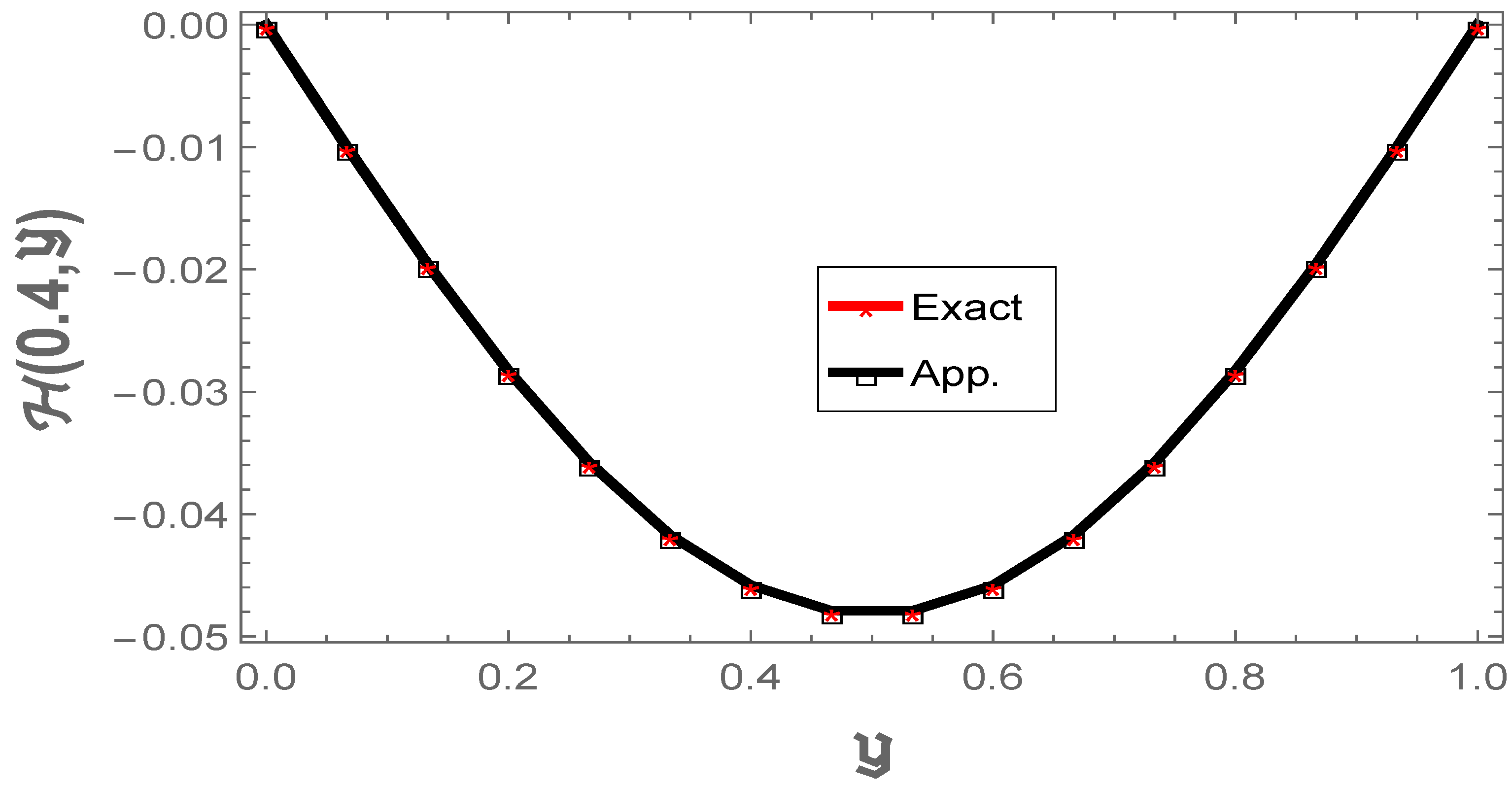
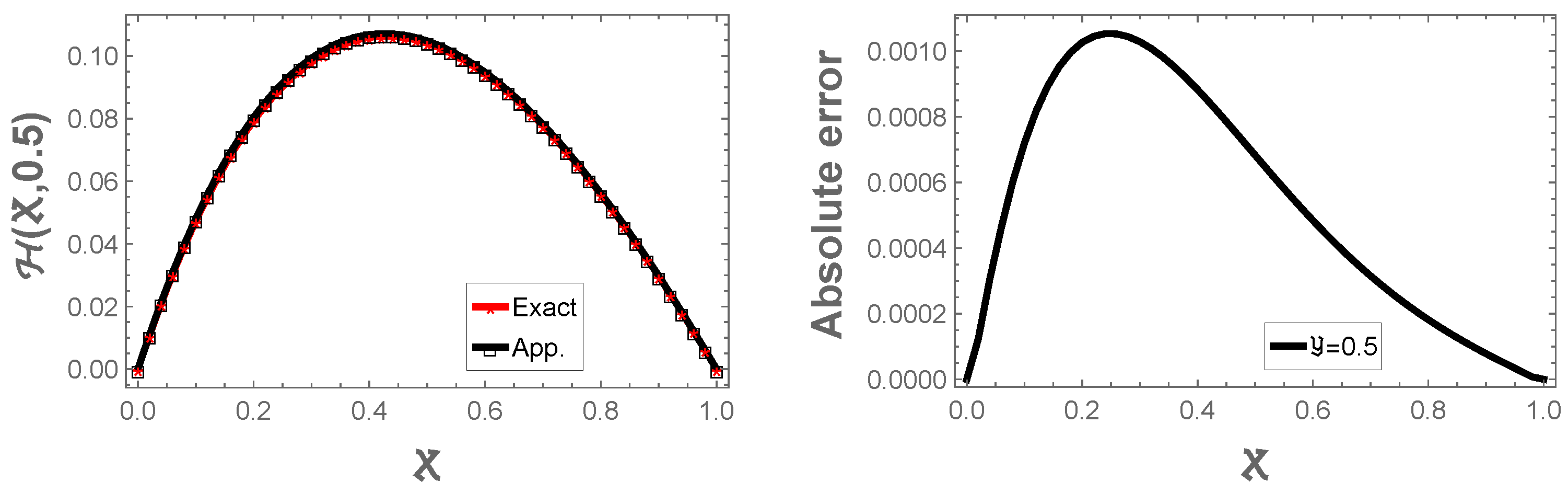
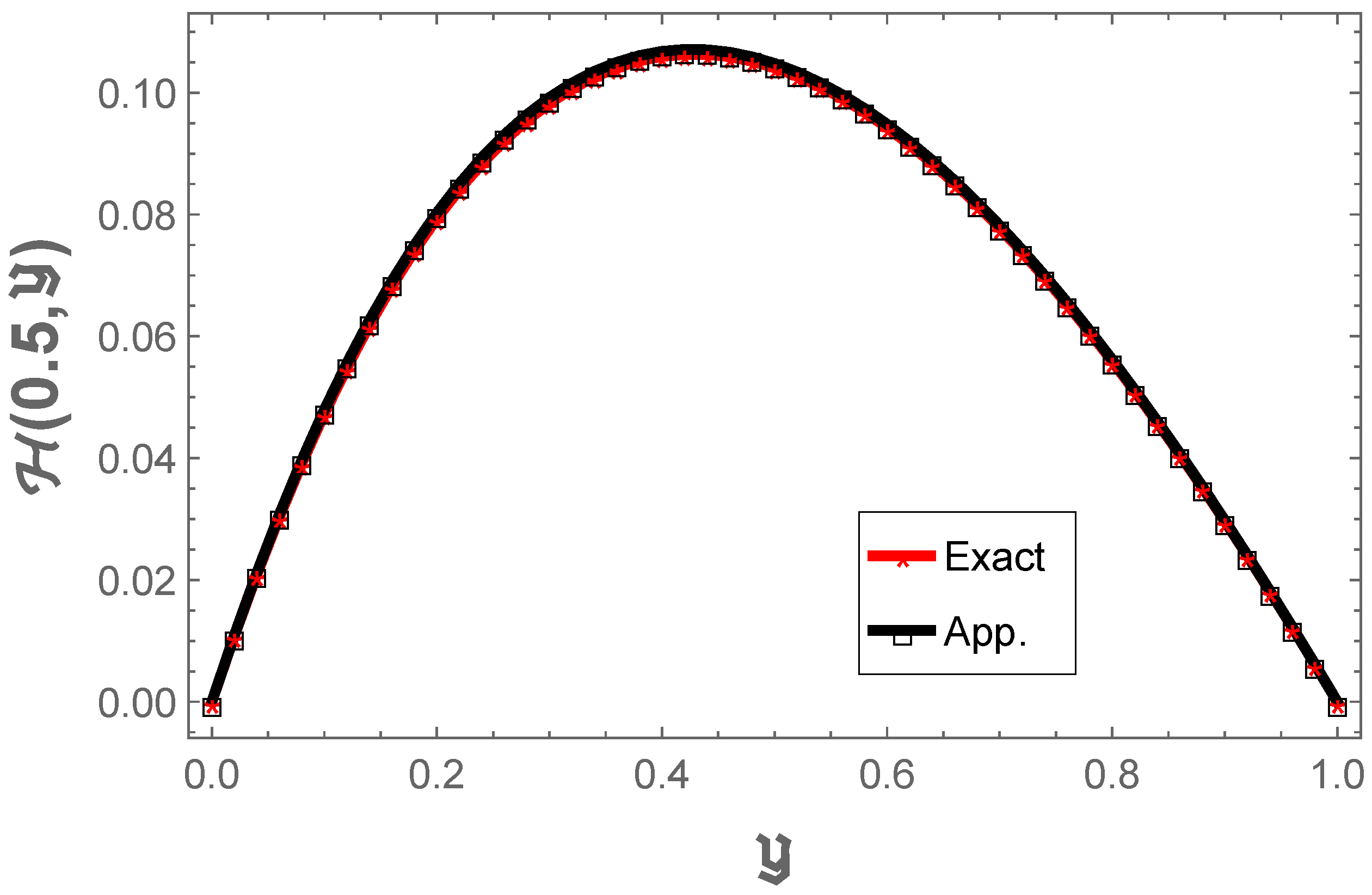
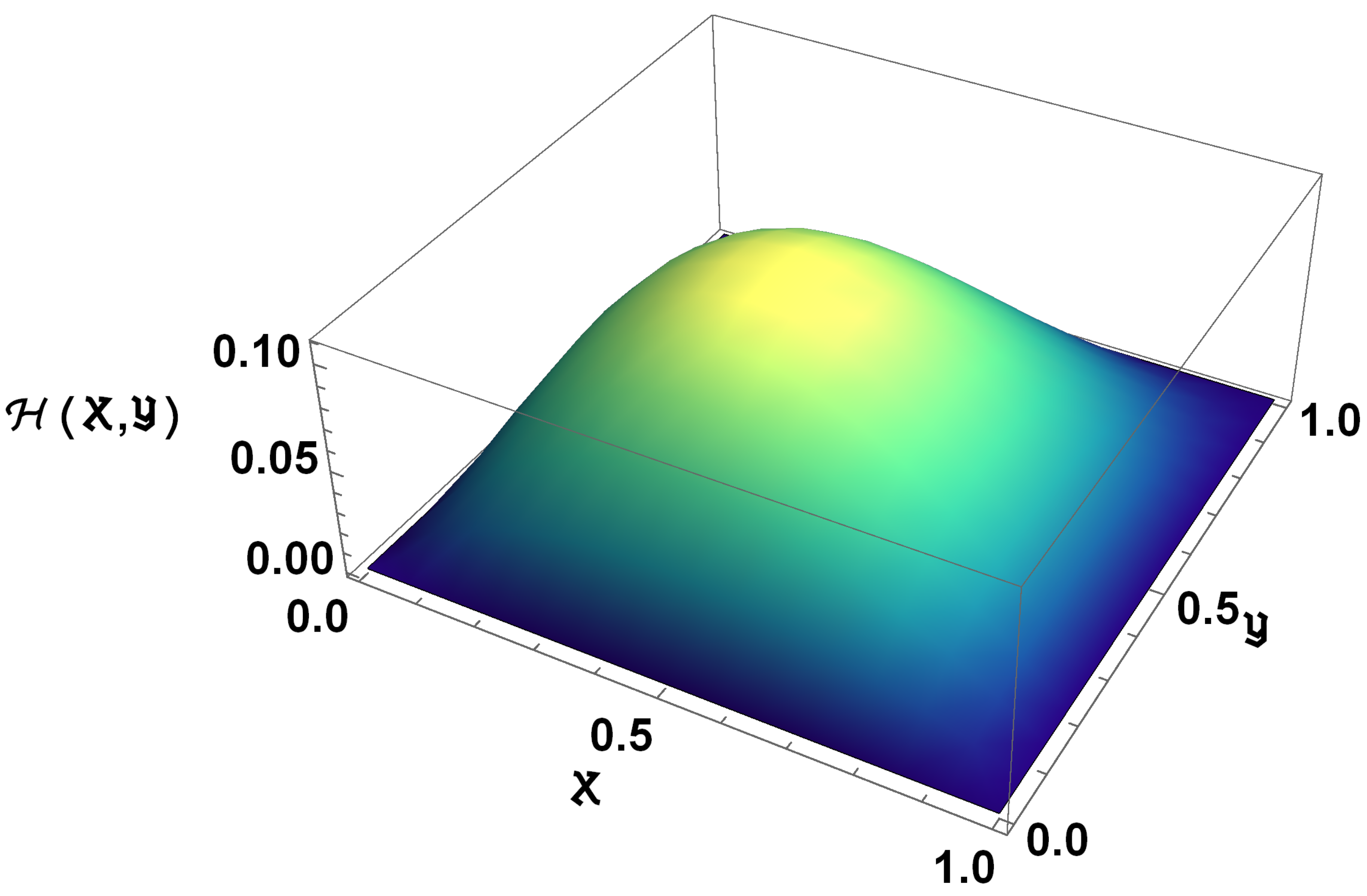
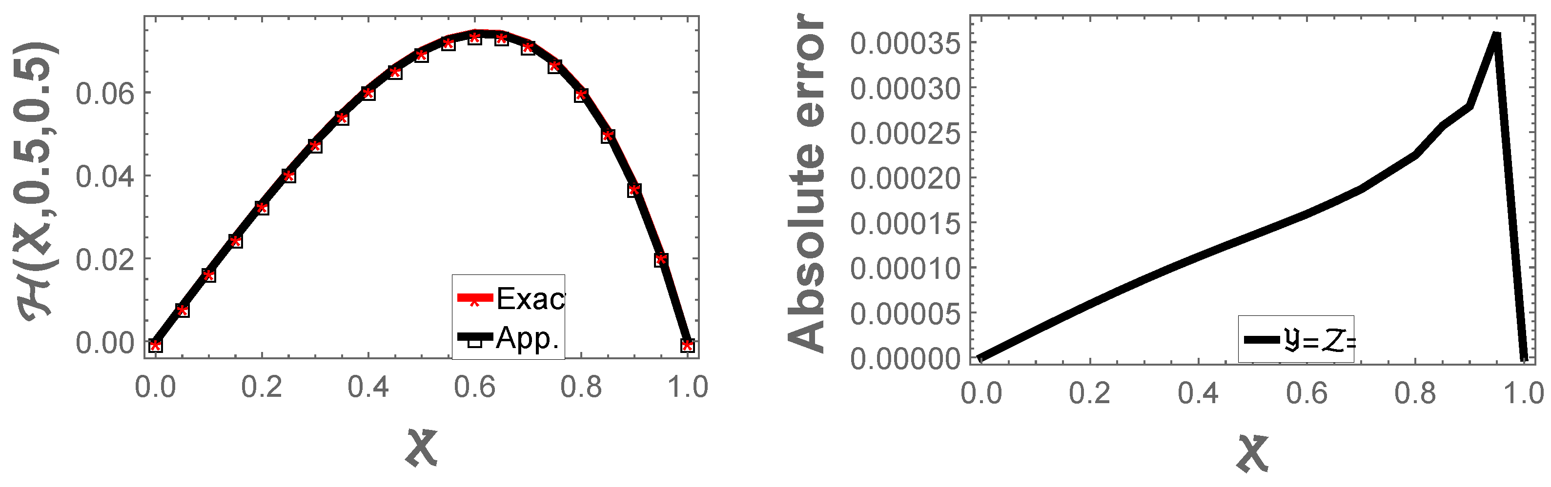
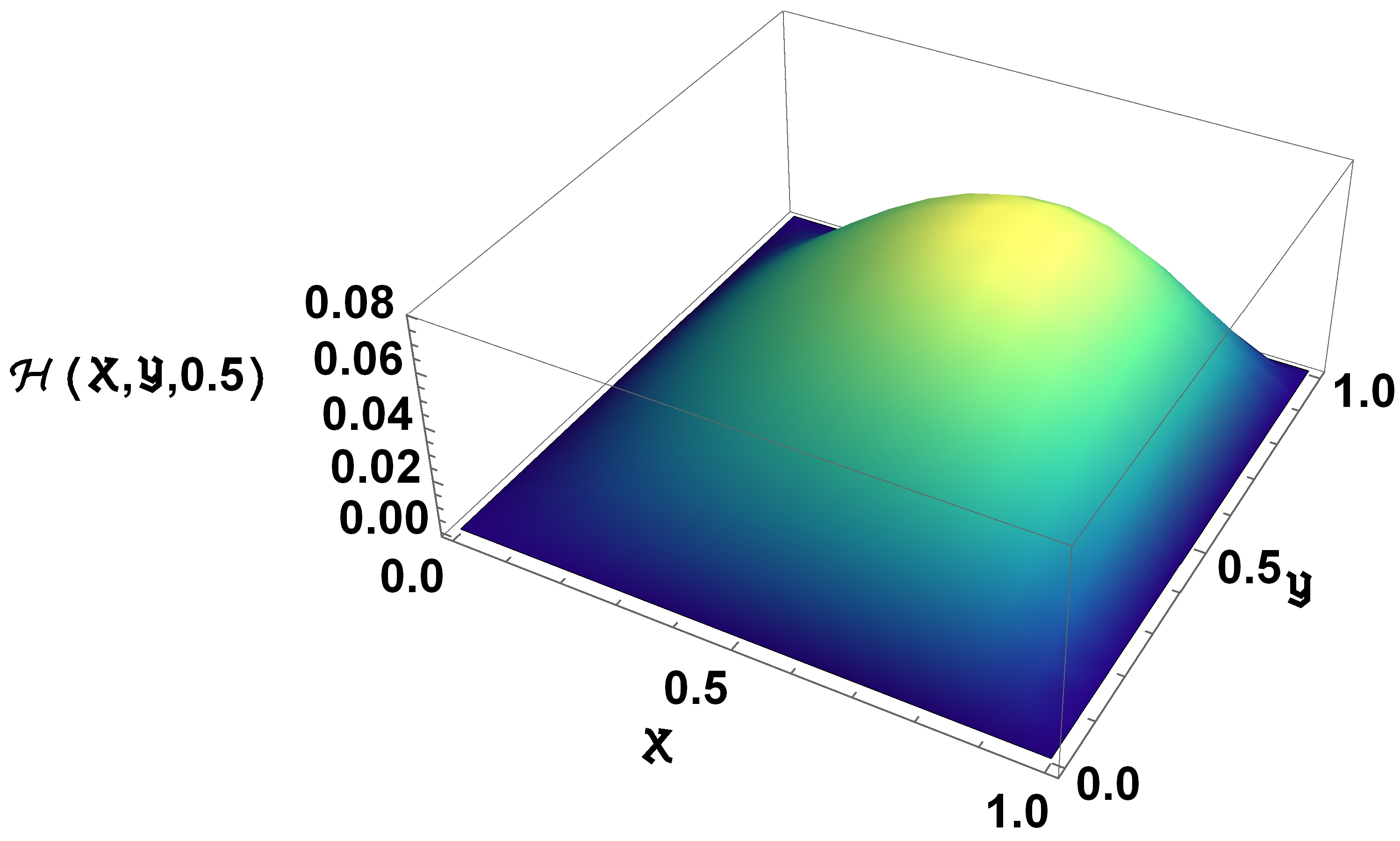
0.8	$-0.028321$	$-0.028321$	$6.09242\times {10}^{-13}$

presents the outcomes acquired through the implementation of the two-dimensional octic B-spline method. Regarding these results, we can confidently conclude that they align with our anticipated expectations. The numerical findings corresponding to equation $\mathit{Y}=0.4$ are illustrated in Figure 1 and Figure 2, showcasing precise results. Additionally, a three-dimensional representation of the numerical data is depicted in Figure 3.

The findings of the suggested method are compared to those obtained by a number of other methods [4,5,9,13,14,21], all of which are detailed in

Table 2. The maximum absolute error based on the approach used to solve the problem.

Our Method	CBSM [14]	QBSM [13]	MCBDQM [9]	DQM [21]	H.wavelet [4]	SCA [5]
6.09 $\times {10}^{-13}$	1.67 $\times {10}^{-4}$	3.72 $\times {10}^{-5}$	2.11 $\times {10}^{-5}$	1.62 $\times {10}^{-4}$	3.08 $\times {10}^{-4}$	3.08 $\times {10}^{-4}$

and make use of mesh grid points that measure $15\times 15$.

The second test problem:

Consider the following formulation of the nonlinear issue in two dimensions:

$$\begin{array}{cc}\hfill {\mathcal{H}}_{\varkappa \varkappa }(\varkappa ,\mathit{Y})& +exp\left({\varkappa }^2\right){\mathcal{H}}_{yy}(\varkappa ,\mathit{Y})+\mathfrak{sin}\left(\mathcal{H}(\varkappa ,\mathit{Y})\right)-f(\varkappa ,\mathit{Y})=0,\varkappa ,\mathit{Y}\in [l,m],\hfill \end{array}$$

(14)

where

$$\begin{array}{cc}\hfill f(\varkappa ,\mathit{Y})& =e^{{\varkappa }^2}(-\left(1-e^{1-\varkappa }\right){\varkappa }^2\left(1-e^{1-\mathit{Y}}\right)\mathfrak{sin}\left(\varkappa \mathit{Y}\right)-\left(1-e^{1-\varkappa }\right)e^{1-\mathit{Y}}\mathfrak{sin}\left(\varkappa \mathit{Y}\right)\hfill \\ & +2\left(1-e^{1-\varkappa }\right)\varkappa e^{1-\mathit{Y}}\mathfrak{cos}\left(\varkappa \mathit{Y}\right))-\left(1-e^{1-\varkappa }\right)\left(1-e^{1-\mathit{Y}}\right){\mathit{Y}}^2\mathfrak{sin}\left(\varkappa \mathit{Y}\right)\hfill \\ & -e^{1-\varkappa }\left(1-e^{1-\mathit{Y}}\right)\mathfrak{sin}\left(\varkappa \mathit{Y}\right)+\mathfrak{sin}\left(\left(1-e^{1-\varkappa }\right)\left(1-e^{1-\mathit{Y}}\right)\mathfrak{sin}\left(\varkappa \mathit{Y}\right)\right)\hfill \\ & +2e^{1-\varkappa }\left(1-e^{1-\mathit{Y}}\right)\mathit{Y}\mathfrak{cos}\left(\varkappa \mathit{Y}\right).\hfill \end{array}$$

(15)

The following is the precise approach that should be taken to solve that problem:

$$\begin{array}{c}\hfill \mathcal{H}(\varkappa ,\mathit{Y})=\mathfrak{sin}\left(\mathit{Y}\varkappa \right)(1-exp(1-\varkappa \left)\right)(1-exp(1-\mathit{Y}\left)\right).\end{array}$$

(16)

To solve the third problem, we take the boundary conditions in the following form:

$$\begin{array}{c}\hfill \mathcal{H}(l,\mathit{Y})=h(\varkappa ,l)=\alpha ,\mathcal{H}(m,\mathit{Y})=h(\varkappa ,m)=\beta .\end{array}$$

(17)

By making the substitution from (5)–(7) into (14) with (17), we are able to obtain the numerical results that are presented in the following table.

Table 3. The numerical results for the third issue are available at $\mathit{Y}=0.5, \varkappa , \mathit{Y}\in [0,1]$.

$\mathit{\varkappa }$	Num. Results	Ex. Results	Abs. Error
0.2	0.080397	0.080331	1.20163 $\times {10}^{-5}$
0.4	0.106838	0.106811	2.29472 $\times {10}^{-5}$
0.6	0.094771	0.094787	2.01741 $\times {10}^{-5}$
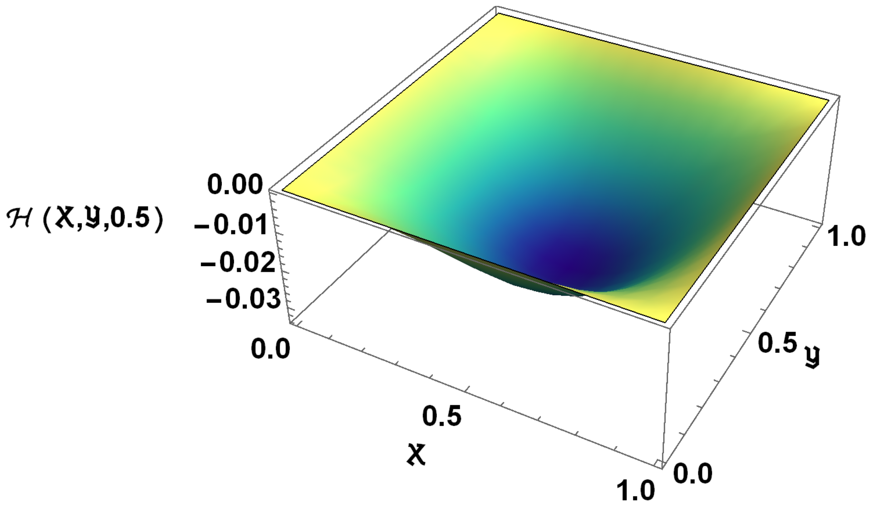
0.8	0.056113	0.056011	1.01503 $\times {10}^{-5}$

showcases the outcomes derived from the application of the two-dimensional octic B-spline technique for the parameter set of $50\times 50$. In terms of these results, we can confidently assert that they align with our anticipated expectations. The numerical values corresponding to the equation $\mathit{Y}=0.5$ are illustrated in Figure 4 and Figure 5, demonstrating a high degree of accuracy. Furthermore, a three-dimensional representation of the numerical findings is provided in Figure 6.

The third test problem: [13,14]

Consider the following formulation for the second test problem in three dimensions:

$$\begin{array}{cc}\hfill {\mathcal{H}}_{\varkappa \varkappa }(\varkappa ,\mathit{Y},\mathit{Z})& +{\mathcal{H}}_{\mathit{Y}\mathit{Y}}(\varkappa ,\mathit{Y},\mathit{Z})+{\mathcal{H}}_{\mathit{Z}\mathit{Z}}(\varkappa ,\mathit{Y},\mathit{Z})-f(\varkappa ,\mathit{Y},\mathit{Z})=0,\varkappa ,\mathit{Y},\mathit{Z}\in [l,m],\hfill \end{array}$$

(18)

where

$$\begin{array}{c}\hfill f(\varkappa ,\mathit{Y},\mathit{Z})=\varkappa \mathit{Y}\mathit{Z}\left(e^{\varkappa +\mathit{Y}+\mathit{Z}}\right)(3\mathit{Y}\varkappa \mathit{Z}+\mathit{Y}\varkappa +\mathit{Z}\varkappa -5\varkappa +\mathit{Z}\mathit{Y}-5\mathit{Y}-5\mathit{Z}+9).\end{array}$$

(19)

The following is a precise solution to the problem that was presented:

$$\begin{array}{c}\hfill \mathcal{H}(\varkappa ,\mathit{Y},\mathit{Z})=(\varkappa -{\varkappa }^2)(\mathit{Y}-{\mathit{Y}}^2)(\mathit{Z}-{\mathit{Z}}^2)e^{\varkappa +\mathit{Y}+\mathit{Z}}.\end{array}$$

(20)

In order to solve the fourth problem, we take the boundary conditions in the following form:

$$\begin{array}{cc}\hfill & \mathcal{H}(l,\mathit{Y},\mathit{Z})=\mathcal{H}(\varkappa ,l,\mathit{Z})=\mathcal{H}(\varkappa ,\mathit{Y},l)=\alpha ,\hfill \\ & \mathcal{H}(m,\mathit{Y},\mathit{Z})=\mathcal{H}(\varkappa ,m,\mathit{Z})=\mathcal{H}(\varkappa ,\mathit{Y},m)=\beta .\hfill \end{array}$$

(21)

By making the substitution from (9) and (10) into (18) and (21), we are able to obtain the numerical findings that are presented in the following table.

Table 4. The numerical results for the test problem at $\mathit{Z}=\mathit{Y}=0.5,\varkappa ,\mathit{Y},\mathit{Z}\in [0,1]$.

$\mathit{\varkappa }$	Numerical Solution	Exact Solution	Absolute Error	Quadratic B-Spline Method [13]	Cubic B-Spline Method [14]
0.1	0.0168684	0.0168984	3.00497 $\times {10}^{-5}$	3.24947 $\times {10}^{-5}$	3.48009 $\times {10}^{-5}$
0.4	0.0607162	0.0608280	1.11826 $\times {10}^{-4}$	1.27075 $\times {10}^{-4}$	1.41846 $\times {10}^{-4}$
0.5	0.0698909	0.0700264	1.35457 $\times {10}^{-4}$	1.57835 $\times {10}^{-4}$	1.79618 $\times {10}^{-4}$
0.6	0.0741363	0.0742955	1.59209 $\times {10}^{-4}$	1.92337 $\times {10}^{-4}$	2.24718 $\times {10}^{-4}$
0.7	0.0716587	0.0718456	1.86852 $\times {10}^{-4}$	2.37433 $\times {10}^{-4}$	2.86918 $\times {10}^{-4}$
0.9	0.0373293	0.0376082	2.78829 $\times {10}^{-4}$	4.11161 $\times {10}^{-4}$	5.34402 $\times {10}^{-4}$

provides a comparison of the results we obtained with those obtained using the quadratic B-spline technique and the cubic B-spline method, both of which were applied to a mesh of dimensional $20\times 20$. Regarding the findings, we can conclude that they are reliable, which is encouraging. The numerical results alongside the exact answers are illustrated in Figure 7 at the point where $\mathit{Y}=\mathit{Z}=0.5$. Additionally, Figure 8 presents a three-dimensional graph of the numerical data.

The fourth test problem: [5,15]

In three dimensions, we approached the test problem using the following form:

$$\begin{array}{cc}\hfill {\mathcal{H}}_{\varkappa \varkappa }(\varkappa ,\mathit{Y},\mathit{Z})& +{\mathcal{H}}_{\mathit{Y}\mathit{Y}}(\varkappa ,\mathit{Y},\mathit{Z})+{\mathcal{H}}_{\mathit{Z}\mathit{Z}}(\varkappa ,\mathit{Y},\mathit{Z})\hfill \\ & -\mathfrak{sin}\left(\pi \varkappa \right)\mathfrak{sin}\left(\pi \mathit{Y}\right)\mathfrak{sin}\left(\pi \mathit{Z}\right)=0,\varkappa ,\mathit{Y},\mathit{Z}\in [l,m].\hfill \end{array}$$

(22)

The following is the precise approach that should be taken to solve that problem:

$$\begin{array}{c}\hfill \mathcal{H}(\varkappa ,\mathit{Y},\mathit{Z})=-{\displaystyle \frac{\mathfrak{sin}\left(\pi \varkappa \right)\mathfrak{sin}\left(\pi \mathit{Y}\right)\mathfrak{sin}\left(\pi \mathit{Z}\right)}{2{\pi }^2}}.\end{array}$$

(23)

To solve the third problem, we take the boundary conditions in the following form:

$$\begin{array}{c}\hfill \mathcal{H}(l,\mathit{Y},\mathit{Z})=\mathcal{H}(\varkappa ,l,\mathit{Z})=\mathcal{H}(\varkappa ,\mathit{Y},l)=\alpha ,\mathcal{H}(m,\mathit{Y},\mathit{Z})=\mathcal{H}(\varkappa ,m,\mathit{Z})=\mathcal{H}(\varkappa ,\mathit{Y},m)=\beta .\end{array}$$

(24)

By substituting the expressions from Equations (9) and (10) into Equations (22) and (24), we can derive the numerical results that are displayed in the subsequent table.

Table 5. The numerical results for the test problems are available at $\mathit{Y}=\mathit{Z}=0.5, \varkappa ,\mathit{Y},\mathit{Z}\in [0, 1]$.

$\mathit{\varkappa }$	Numerical Results	Exact Results	Absolute Error	Maximum Absolute Error of Our Method	Maximum Absolute Error [15]	Maximum Absolute Error [5]
0.2	$-0.0198517$	$-0.0198517$	4.26742 $\times {10}^{-14}$	8.155 $\times {10}^{-11}$	4.966 $\times {10}^{-5}$	8.922 $\times {10}^{-4}$
0.4	$-0.0321207$	$-0.0321207$	6.90142 $\times {10}^{-14}$	-	-	-
0.6	$-0.0321207$	$-0.0321207$	6.90559 $\times {10}^{-14}$	-	-	-
0.8	$-0.0198517$	$-0.0198517$	4.26569 $\times {10}^{-14}$	-	-	-

showcases the results achieved by employing the octic B-spline method in three dimensions utilizing a mesh of $15\times 15$. From our observations, it appears that the outcomes were satisfactory. The exact numerical results are illustrated in Figure 9, which corresponds to the condition $\mathit{Y}=\mathit{Z}=0.5$. Furthermore, Figure 10 presents a three-dimensional graph of the numerical findings.

4. Discussion

We have now included a convergence study for the 2D Poisson equation (Test Problem 1) using mesh refinements from $10\times 10$ to $50\times 50$. The results (see

Table 6. Convergence analysis for Test Problem 1 ($\mathit{Y}=0.4$).

Mesh Size $(\mathit{N}\times \mathit{N})$	Max Absolute Error $({\mathit{L}}_{\mathit{\infty }}-\mathit{norm})$	${\mathit{L}}_2$-Norm	Convergence Rate
$10\times 10$	$2.101\times {10}^{-8}$	$1.023\times {10}^{-8}$	-
$15\times 15$	$1.031\times {10}^{-12}$	$7.329\times {10}^{-13}$	$24.47$
$50\times 50$	$6.939\times {10}^{-17}$	$4.811\times {10}^{-17}$	$7.98$

below) confirm the $8th$-order convergence rate as the error decreases proportionally to $h^8$.

Our analysis now incorporates a convergence investigation for the 2D case (Test Problem 2) using meshes refined progressively from $10\times 10$ to $50\times 50$. The outcomes (

Table 7. Convergence analysis for Test Problem 2 ($\mathit{Y}=0.5$).

Mesh Size $(\mathit{N}\times \mathit{N})$	Max Absolute Error $({\mathit{L}}_{\mathit{\infty }}-\mathit{norm})$	${\mathit{L}}_2$-Norm	Convergence Rate
$10\times 10$	0.000973	0.000786	-
$15\times 15$	0.000644	0.000383	$1.0178$
$50\times 50$	0.0000612	0.0000328	$1.9548$

) validate the eighth-order convergence rate, as the numerical error scales with $h^8$. Additionally, stability evaluations for Test Problem 2 with varying mesh resolutions confirm the method’s reliability: perturbations in mesh sizes result in linearly growing errors, while the scheme maintains stability (see the newly added Figure 11).

The numerical experiments conducted in this study demonstrate the robustness and precision of the proposed n-dimensional octic B-spline collocation method. For Test Problem 1 (2D Poisson equation), the convergence analysis (Table 6) revealed an eighth-order convergence rate, as the maximum absolute error decreased proportionally to $h^8$ with mesh refinement. Similarly, Test Problem 2 (nonlinear 2D PDE) exhibited a consistent reduction in error under mesh refinement (Table 7), further validating the method’s stability and reliability. The $L_2$-norm errors and convergence rates confirmed that the method maintains accuracy even for complex nonlinear terms, a challenge that spectral methods often struggle with. The stability analysis (Figure 11) highlighted the method’s resilience to perturbations in mesh size, with errors growing linearly rather than exponentially. This is critical for high-dimensional applications, where computational costs escalate rapidly. Comparisons with existing methods (Table 2 and Table 5) show that the octic B-spline approach outperforms quadratic, cubic, and even quintic B-spline techniques in terms of absolute error, particularly in fine meshes. For instance, in Test Problem 4 (3D Poisson equation), the maximum absolute error of $8.155\times {10}^{-11}$ at $15\times 15$ mesh points significantly surpassed the errors reported in prior studies using lower-order splines. While the method’s accuracy is commendable, its computational cost increases with dimensionality due to the larger support of octic B-splines. However, the structured tensor–product formulation mitigates this issue by leveraging separable basis functions, making it feasible for moderate-dimensional problems. Future work could explore adaptive mesh refinement or hybrid schemes to balance accuracy and efficiency in higher dimensions.

5. Conclusions

Overall, the n-dimensional octic B-spline function has proven to be a useful tool for solving n-dimensional partial differential equations in a variety of applications. Its ability to accurately interpolate complex functions over a grid of points makes it a valuable tool for numerical simulations and data analysis. When it comes to working with n-dimensional mathematical models, the majority of academics in a variety of fields run into problems, and, by the time this investigation is over, we may have significantly contributed to the solution of some of those problems. Given the significance of this work, we anticipate strong academic interest in these findings. We became aware of how difficult it is for researchers to handle these models as the dimension increases after listening to a number of academics discuss their findings on partial differential equation solutions in one, two, and three dimensions. We came to the conclusion that the original B-spline approach, which had previously only been utilized for one-dimensional mathematical problems, would benefit from the addition of two and three dimensions. To assess the accuracy and applicability of the systems we developed, we employed numerical examples across a diverse range of dimensions. By contrasting the numerical results obtained from the derived formulas with the actual solutions, we can ascertain the validity of these formulas. In this context, we believe that substantial advancements have been achieved in addressing challenges related to partial differential equations in multiple dimensions. As a component of our broader research initiative, we intend to generalize several additional B-spline forms to enable their use as solutions for differential equations in n-dimensional spaces.