Abstract
With the advancement of science and technology, industrial robots have become indispensable equipment in advanced manufacturing and a critical benchmark for assessing a nation’s manufacturing and technological capabilities. Enhancing the reliability of industrial robots is therefore a pressing priority. This paper investigates the drive system of industrial robots, modeling it as a series system comprising multiple components (n) with a repairman who operates under a single vacation policy. The system assumes that each component’s lifespan follows an exponential distribution, while the repairman’s repair and vacation times adhere to general distributions. Notably, the repairman initiates a vacation at the system’s outset. Using the supplementary variable method, a mathematical model of the system is constructed and formulated within an appropriate Banach space, leading to the derivation of the system’s abstract development equation. Leveraging functional analysis and the -semigroup theory of bounded operators, the study examines the system’s adaptability, stability, and key reliability indices. Furthermore, numerical simulations are employed to analyze how system reliability indices vary with parameter values. This work contributes to the field of industrial robot reliability analysis by introducing a novel methodological framework that integrates vacation policies and general distribution assumptions, offering new insights into system behavior and reliability optimization. The findings have significant implications for improving the design and maintenance strategies of industrial robots in real-world applications.
MSC:
34A30; 34D20; 47D06; 47A10; 47B01; 60H30
1. Introduction
With the rapid development of science and technology, industrial robots have been widely adopted across various industries, particularly in high-intensity, repetitive, and harsh-environment tasks, where their demand has become increasingly prominent. Industrial robots not only significantly enhance production efficiency but also accomplish high-precision and high-risk tasks that are challenging for humans, making them indispensable core equipment in modern manufacturing. However, as industrial robots become more prevalent in production, their reliability issues have also become increasingly apparent. Failures in industrial robot systems can lead to production line shutdowns, safety incidents, and declines in product quality, thereby severely impacting production efficiency, operational costs, and workplace safety. Therefore, improving the safety, stability, and reliability of industrial robot systems has become a critical focus for both academia and industry [1].
The core component of industrial robots is the drive system, whose reliability directly determines the performance of the entire robot system. Failures in the drive system can lead to equipment downtime, resulting in economic losses. For example, in high-precision industries such as automotive manufacturing, even minor faults in the drive system can cause the entire production line to shut down, leading to significant production losses. Furthermore, as manufacturing transitions toward intelligence and automation, the role of industrial robots in the production chain has become increasingly critical. Their reliability directly impacts a company’s competitiveness and market reputation.
Moreover, improving the reliability of industrial robot drive systems holds significant value for manufacturers, operators, and stakeholders across the entire industry ecosystem. For manufacturers, highly reliable drive systems can reduce after-sales maintenance costs and enhance market competitiveness. For operators, reliable systems can minimize downtime, improve production efficiency, and lower operational costs. For workers, increased reliability translates to a safer working environment and reduced risk of accidents. For consumers, highly reliable industrial robots ensure stable and consistent product quality, thereby boosting consumer trust and satisfaction. Therefore, enhancing the reliability of industrial robot drive systems is not only a technological imperative but also a shared focus for industry stakeholders.
Drive systems can generally be categorized into three types: hydraulic, pneumatic, and electrical drivers. Among these, the electrical driver is typically divided into seven modules based on the roles and functions of its various components (Figure 1). Each module, in turn, comprises multiple components. If any single component fails, the entire drive system will be compromised. As a result, the drive system can be modeled as a series system composed of several interconnected components (Figure 2).
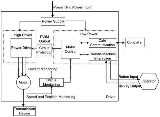
Figure 1.
Each structural module of the electric driver and its relationship diagram.
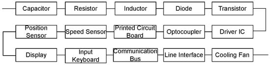
Figure 2.
Electrical drive system reliability block diagram.
In recent years, many scholars have conducted extensive research on the reliability analysis of repairable systems (see [2,3,4,5,6]). For example, literature [2] studied the steady-state solution of the system using the supplementary variable method and Laplace transform and derived the system’s reliability and failure frequency within the interval (0, t]. Literature [3] investigated the reliability of a parallel repairable system with a repairman who follows a single vacation policy. The literature [4] established a mathematical model of the robot safety system by applying stochastic process theory and the supplementary variable method. The study further analyzed the system operator’s spectrum using functional analysis and strongly continuous semigroup theory, ultimately proving the asymptotic stability of the solution.
Early research assumed that system components were repaired immediately after failure (see [7,8,9,10]); however, this assumption did not hold in practice. Due to various circumstances, repairmen are not always available in the system. Therefore, a repairable system incorporating various vacation policies for repairmen has been proposed (see [11,12,13,14,15]). For instance, Y. L. Li and G. Q. Xu [15] introduced a parallel repairable degradation system consisting of two similar components and a repairman who can take a single vacation. Subsequently, to further enhance the system’s reliability, a large number of studies have been conducted on the maintenance strategies of repairable systems (see [16,17,18]). Nevertheless, as the application scenarios of industrial robots become increasingly complex and diverse, their reliability analysis still faces numerous challenges. For instance, how to accurately model maintenance strategies in multi-component series systems, how to optimize system stability, and how to validate the practical applicability of theoretical results through numerical simulations are all critical issues that need to be addressed. Notably, the connection between device-failure statistics and reset process statistics, as an emerging research direction (see [19]), provides a novel perspective for reliability analysis.
Based on the above research, this paper focuses on the reliability of a series system composed of various components of the electrical drive, which is the core component of industrial robots. Due to the large number of components in the electrical drive, we first examine an n-component series repairable system with a repairman who follows a single vacation policy. A detailed description of the system is provided in Section 2. In particular, it is assumed that the repairman takes a vacation at the initial moment, and the repair equipment does not fail during the repair process. This paper introduces a single vacation policy for the repairman, which better aligns with real-world application scenarios, as maintenance personnel are not always on standby. Additionally, this paper focuses on a multi-component series repairable system, enabling a more comprehensive analysis of the interactions between components and their impact on the overall system reliability. However, a limitation of this study is the assumption that the repair equipment does not fail during the repair process, which may not fully hold in practical environments. Future research could further incorporate the failure probability of repair equipment to enhance the model’s applicability. Moreover, exploring multiple vacation policies and other complex vacation strategies for the repairman could provide a more comprehensive reflection of the dynamic allocation of maintenance resources in real-world scenarios.
This study employs a combination of mathematical modeling, -semigroup theory, and numerical simulation to systematically analyze the well-posedness, stability, and reliability indices of the series repairable system. Among these, -semigroup theory provides a theoretical guarantee for the well-posedness of the system model and the stability of its solutions, while spectral analysis reveals the long-term behavior and stability conditions of the system by studying the spectral properties of the system operator. Specifically, the mathematical model of the system is first established using the supplementary variable method and formulated within an appropriate Banach space. Subsequently, the well-posedness of the system is discussed using -semigroup theory, and the stability results are derived through spectral analysis of the system operator. Finally, several reliability indices of the system are presented, and the variation in these indices with parameter values is analyzed through numerical simulation, thereby providing practical guidance for real-world applications.
2. Mathematical Modelling
In this section, we present the system under consideration and derive its dynamic equations.
Consider a driver system composed of n series-connected components, such as capacitors, resistors, and inductors, along with a single repairman. The repairman is allowed to take vacations. Additionally, the system operates under the following assumptions:
Assumption 1.
Initially, all components are new and the drive system is in a working state. When any component fails, the system ceases to operate until the faulty component is repaired, after which the drive system resumes functioning. At the initial moment, the repairman is on vacation.
Assumption 2.
The lifetimes of the n components follow exponential distributions with parameters . The repair times for the n components and the vacation time of the repairman follow general distributions with repair rates and vacation rate , respectively. It is assumed that components after repair are “as good as new”. All the aforementioned random variables are mutually independent.
It should be noted that the exponential distribution is typically used to describe the lifetime distribution of components with a constant failure rate (i.e., the memoryless property). For certain components, especially during the early stages of their service life, the failure rate often remains constant. This means that the probability of failure does not increase over time but instead stabilizes at a certain level. Therefore, in such cases, the exponential distribution is a reasonable choice. To further illustrate this assumption, the probability density function (PDF) of the exponential distribution under different parameters is provided below (Figure 3).
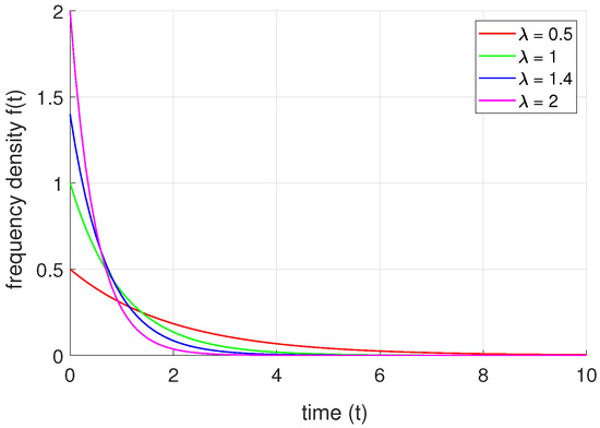
Figure 3.
Probability density function (PDF) of the exponential distribution under different parameters.
Under the above assumptions, we can divide the system into the following states:
State 0: The drive system is working and the repairman is taking his vacation;
State w: The drive system is working and the repairman is waiting in the system;
State i: Component is fail and the repairman is taking his vacation;
State : Component is being repaired.
We now introduce the random variable , which at time t takes values from the state set . Here, indicates that the system is in state k at time t. Additionally, the random variables and , defined at time t, take values in the interval . These variables represent the elapsed repair time for the i-th component and the elapsed vacation time of the repairman, respectively. Consequently, the probability or probability density functions of the drive system in all states are as follows:
Thus, the dynamic behavior of the drive system is governed by the partial differential equations
with the boundary conditions
and the initial conditions
with .
3. Well-Posedness of the System (1)–(3)
In this section, we formulate systems (1) and (2) within an appropriate Banach space and analyze their fundamental properties. Based on the practical background of the model, it is assumed that and satisfy
and take the state space equipped with the norm
where . Obviously, is a Banach space.
Now we define the operator in by
with domain
Obviously, is a linear operator in .
By employing the notation defined earlier, we can express (1) and (2) as an abstract evolutionary equation in Banach space :
where .
Firstly we have the following result.
Theorem 1.
(1) is a closed and densely defined linear operator on ;
(2) is a dissipative operator in and for all .
Proof.
The first assertion follows from a straightforward verification. For the second assertion, we proceed by dividing the proof into the following two steps.
Step 1. We demonstrate that is a dissipative operator in .
In fact, for any we define a function group
where .
Obviously, , and Q ∈  , where .
Moreover, we have
Since
using the boundary condition in we get
Therefore, is a dissipative operator in .
Step 2. We prove that .
For any and with , we consider the resolvent equation , where , that is,
with boundary conditions
Solving the differential equations in (7) leads to the following general solutions:
where
By the assumption on and , we have
so .
Moreover, from (7) we can find that
are finite values, so and the boundary conditions in (8) are meaningful.
By substituting expression in (9) into the boundary conditions (8) leads to an algebraic equation about an unknown parameter .
where
Denoted by the coefficient matrix of (10) and by the determinant of , i.e.,
and .
Since it holds the following inequalities for
the matrix is column strictly diagonal dominant and hence . Therefore, for , Equation (10) has a unique solution . Consequently, for each , there exists a unique solution such that . By the closed operator theorem, exists and is bounded. Thus . □
As a direct consequence of Theorem 1 and semigroup generation theory (see [20]), we obtain the following result.
Theorem 2.
Let and be defined as before. Then generates a semigroup of contractions on . Hence the Equation (6) is well-posed.
Next, we investigate the existence of positive solutions to Equation (6). Let be a real Banach space, and let denote the set defined by
The set is known as the positive cone of , and constitutes a Banach lattice. For further details on Banach lattices, positive cones, and positive semigroups, see [21].
Theorem 3.
Let and be defined as before and be the semigroup generated by . Then is a positive semigroup and satisfies for and any vector .
Proof.
Let denoted the semigroup generated by . We demonstrate that is a positive semigroup and satisfies for any positive vector .
Step 1. is a positive semigroup on .
Based on the theory of positive semigroups (see [21]), generates a positive semigroup of contractions if and only if is a dispersive and . From Theorem 2 we only need to show that is a dispersive operator.
For any , we take
where
we have
By performing a calculation analogous to that in the proof of Theorem 1, we demonstrate that . This proves that is a dispersive operator, and hence, constitutes a positive operator semigroup on .
Step 2. For any , it holds that , .
Let . By the positive semigroup property of , is a classical solution to system (6). Set
Then satisfy Equations (1) and (2) ((1) and (2) are in Section 2).
Moreover, the norm of is
Thus, we have
that implies is constant, so it holds that , . The proof is then complete. □
4. Stability of the System
This section focuses on the stability analysis of system (6), which is equivalent to systems (1) and (2) presented in Section 2.
Theorem 4.
Let and be defined as before, then is simple eigenvalue of . Moreover if for any , it holds that
Then
Proof.
The proof proceeds in two steps:
Step 1. 0 is a simple eigenvalue of .
Let us consider the equation , with , i.e.,
Solving the differential equations in (14) yields
Substituting them into the boundary conditions (2) ((2) is in Section 2) leads to a homogenous algebraic equation about the unknown parameter , i.e.,
we have
so we obtain , this means that the equation has a non-zero solution. A direct calculation shows that
So 0 is an eigenvalue of with geometric multiplicity one and are given by (18) is the eigenvector of corresponding to 0.
Next, we will prove that the algebraic multiplicity of 0 is 1. A direct computation shows that the dual operator of is of the form
where and
Obviously, and , so 0 is an eigenvalue of and is a corresponding eigenvector. Using (18) we obtain
Therefore, 0 is a simple eigenvalue of .
Step 2. .
For , we consider the resolvent equation , we obtain
so
By the assumption of the theorem, we have
for any , so and
is finite. So we can prove
Similarly, we can show that .
From the preceding analysis, we derive the following conclusion:
Theorem 5.
Let and be defined as before. Then the following statements are true:
(1) The operator generates a positive semigroup of contractions .
(2) For any initial value , there is a unique dynamic solution . In particular, is also positive when is positive.
(3) The system (1) has a positive steady-state solution which is given by (18) and is chosen such that , which is the positive eigenvector corresponding to the eigenvalue 0 of the operator . For any , we have
where and is the initial value, the dynamic solution converges to the non-negative steady-state solution in the sense of norm in .
5. Some Indices of the System
This section focuses on analyzing key reliability indices of the system. Using numerical analysis, we explore the dependence of the drive system’s reliability indices on variations in system parameters.
5.1. Indices of Reliability of the System
Firstly, we can obtain the positive eigenvector corresponding to the eigenvalue 0 (). In fact, we assume that in (18), then the following functions
are positive functions and is an eigenvector of corresponding to eigenvalue 0.
For the definitions of steady-state availability and steady-state failure frequency, we refer the reader to [22]. From this, we obtain the following: statements.
Theorem 6.
The steady-state availability of the system is
and the frequency of the steady-state failure is
and the steady-state probability of the repairman is vacation is
where,
5.2. Numerical Analysis
As previously demonstrated, the system is modeled as a series configuration of n components. For the purpose of this analysis, we assume .
Due to the large number of parameters, we first set some parameter values and , as well as the value ranges of parameters and . Then, the range of the values for the average of and is calculated. Finally, provide the variation in reliability indicators and with respect to the average values of and .
The parameter values are given as follows:
and
So, the average values of and are denoted as and , respectively, with value ranges of [1.27, 1.45] and [1.72, 1.90].
Figure 4 and Figure 5 and Table 1 and Table 2 illustrate the variation patterns of the system reliability indices , , and with respect to the average repair rate and mean lifetime rate .
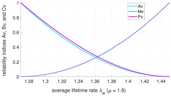
Figure 4.
The variation in reliability indices , , and with respect to the average lifetime rate .
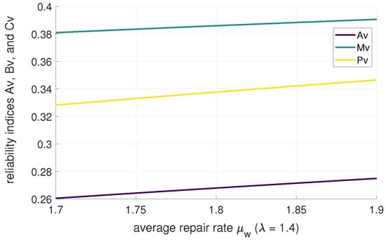
Figure 5.
The variation in reliability indices , , and with respect to the average repair rate .

Table 1.
The variation in reliability indices , , and with respect to the average lifetime rate .
Table 2.
The variation in reliability indices , , and with respect to the average repair rate .
Furthermore, Figure 6, Figure 7 and Figure 8 and Table 3 demonstrate the co-variation patterns of system reliability indices , , and with respect to parameters and .
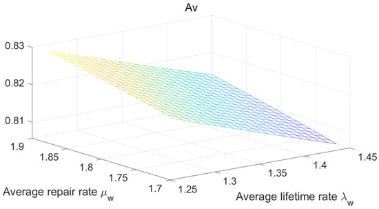
Figure 6.
The variation in reliability indices with respect to the average Lifetime Rate and the the average repair rate .
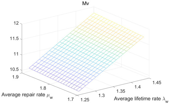
Figure 7.
The variation in reliability indices with respect to the average Lifetime Rate and the the average repair rate .
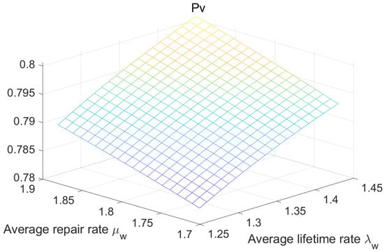
Figure 8.
The variation in reliability indices with respect to the average lifetime rate and the the average repair rate .
Table 3.
The variation in reliability indices , , and with respect to the average rates of parameters (,).
The following can be seen from the above figures and tables:
(1) The stability availability of the drive system decreases with the increase in the average lifetime rate , and increases with the increase in the average repair rate .
(2) The steady-state fault frequency of the drive system increases with the increase in the average lifetime rate and the average repair rate .
(3) The steady-state probability of the repairman’s vacation decreases with the increase in the average lifetime rate , and increases with the increase in the average repair rate .
Based on the above conclusions, we provide practical recommendations for manufacturers or engineers to improve the steady-state availability of the drive system, reduce the steady-state failure frequency, and optimize the repairman’s vacation policy. The specific recommendations are as follows:
(i) Improving System Steady-State Availability ()
(1) Select high-reliability components: Manufacturers should prioritize components with smaller lifespan parameters () to extend the system’s fault-free operation time.
(2) Optimize maintenance strategies: By increasing the repair rate , system downtime can be reduced. Engineers can take the following measures:
(a) Establish a rapid-response maintenance team to ensure timely repairs when failures occur.
(b) Adopt modular designs to facilitate quick replacement of faulty components.
(ii) Reducing Steady-State Failure Frequency ()
(1) Minimize the use of high failure rate components: Manufacturers should avoid using components with shorter lifespans or higher failure rates, especially in critical parts. For example, in drive systems, high-quality gearboxes and bearings should be selected to reduce failure frequency.
(2) Balance repair rate and failure rate: While increasing the repair rate can shorten downtime, an excessively high repair rate may mask fundamental issues in system design. Therefore, engineers should optimize system design to reduce the likelihood of failures while improving the repair rate.
(iii) Optimizing the Repairman’s Vacation Policy
(1) Rational allocation of maintenance resources: Manufacturers can arrange the repairman’s vacation time based on trends in system failure and repair rates. For example, during periods of lower failure rates (smaller ()), the repairman’s vacation time can be appropriately increased, while during periods of higher failure rates, the maintenance team should remain on standby.
(2) Dynamic adjustment of maintenance strategies: By monitoring the system status in real time, the allocation of maintenance resources can be dynamically adjusted. For example, during periods of higher repair rates , the number of maintenance personnel can be reduced to lower labor costs.
From the above analysis, it can be seen that applying this model not only improves the system’s steady-state availability () and reduces the steady-state failure frequency (), but also effectively minimizes system downtime and lowers maintenance costs, thereby significantly enhancing the overall profitability of the system.
Furthermore, there are numerous cases of industrial robots applying this reliability model in real-world manufacturing environments. Taking the automotive manufacturing industry as an example, welding robots are typical representatives of high-intensity and high-precision operations, and the reliability of their electrical drive systems directly impacts production line efficiency and product quality. If welding robots frequently fail during continuous operation, it can lead to production line downtime, thereby affecting production schedules. Analysis reveals that the primary causes of failure are the shorter lifespans of capacitors and resistors in the electrical drive system (higher )) and longer repair response times (lower ).
6. Conclusions
In light of the recent development trends in robotics and the growing demands across various industries, this paper focuses on the reliability of industrial robot drive systems. Analysis of the drive system’s reliability block diagram reveals that the system is fundamentally a series configuration comprising multiple components. Consequently, we examined a repairable series system consisting of n components and a repairman who takes a single vacation. Assuming that both repair times and vacation times follow general distributions, we developed a mathematical model for this system and employed semigroup theory to analyze the stability and reliability of the drive system.
In numerical analysis, since the system is composed of multiple different components in series and involves multiple variables. So, from an overall perspective, we considered the variation in the reliability index with respect to the average values of and , and obtained conclusions consistent with reality. The steady-state availability of the drive system decreases as each component’s lifetime parameter i (i = 1, ⋯, 10) increases, and increases as the repair rate increases. Additionally, when the lifetime parameter of the components increases, the possibility of component failure increases, and thus the probability of the repairman taking a vacation decreases; when the repair rate increases, the steady-state probability of the repairman taking a vacation correspondingly increases.
Author Contributions
Conceptualization, Y.L., G.X. and Y.W.; formal analysis, Y.L., G.X. and Y.W.; investigation, Y.L., G.X. and Y.W.; writing—review and editing, Y.L., G.X. and Y.W. All authors have read and agreed to the published version of the manuscript.
Funding
This research is supported by the National Natural Science Foundation of China grant NSFC-12161071.
Data Availability Statement
The data are contained within this article.
Conflicts of Interest
The authors declare that they have no conflicts of interest.
References
- Fazlollahtabar, H.; Niaki, S.T.A. Reliability Models of Complex Systems for Robots and Automation; CRC Press: Boca Raton, FL, USA, 2017. [Google Scholar]
- Cheng, J.; Tang, Y.H.; Yu, M.M. Reliability of unidirectional closed three-part series and parallel cold storage repairable system. Math. Appl. 2017, 30, 27–39. [Google Scholar]
- Li, Y.L.; Xu, G.Q. Analysis of two components parallel repairable system with vacation. Commun.-Stat.-Theory Methods 2021, 50, 2429–2450. [Google Scholar]
- Hu, L.M.; Yue, D.Q.; Ma, Z.Y. Availability analysis of a repairable series-parallel system with redundant dependency. Commun. -Stat.-Theory Methods 2018, 33, 446–460. [Google Scholar] [CrossRef]
- Qiao, X.; Feng, B.L.; Ma, D. Asymptotic Stability Analysis of Three Robot Safety System Models with Warning Function Analysis. Pract. Underst. Math. 2021, 51, 138–145. [Google Scholar]
- Qiao, X.; Ma, D.; Guo, S. Reliability Analysis and Numerical Simulation of the Five-Robot System with Early Warning Function. Axioms 2025, 14, 113. [Google Scholar] [CrossRef]
- Chen, W.L. System reliability analysis of retrial machine repair systems with warm standbys and a single server of working breakdown and recovery policy. Syst. Eng. 2018, 21, 59–69. [Google Scholar]
- Ke, J.C.; Liu, T.H.; Yang, D.Y. Modelling of Machine Interference Problem with Unreliable Repairman and Standbys Imperfect Switchover. Reliab. Eng. Syst. Saf. 2018, 174, 12–18. [Google Scholar]
- Guo, L.N.; Xu, H.B.; Gao, C. Stability analysis of a new kind n-unit series repairable system. Appl. Math. Model. 2011, 35, 202–217. [Google Scholar]
- Jau, C.; Dong, Y.Y.; Shey, H.S. Availability of a repairable retrial system with warm standby components. Int. J. Comput. Math. 2013, 11, 2279–2297. [Google Scholar]
- Wang, G.R.; Hu, L.M.; Hu, L.M. Reliability modeling for a repairable (k1, k2)-out-of-n: G system with phase-type vacation time. Appl. Math. Model. 2021, 91, 311–321. [Google Scholar] [CrossRef]
- Muhtar, M.; Haji, A.; Rozi, M. Semigroup method for a deteriorating system with multiple vacations of a repairman. Semigroup Forum 2021, 102, 477–494. [Google Scholar] [CrossRef]
- Wang, J.Y.; Ye, J.M.; Ma, Q.R. An extended geometric process repairable model with its repairman having vacation. Ann. Oper. Res. 2022, 311, 401–415. [Google Scholar]
- Qi, X.P.; Haji, A.; Muhtar, M. Dynamic Analysis of a Deteriorating System with Single Vacation of a Repairman. Acta Math. Appl. Appl.-Sin.-Engl. Ser. 2022, 38, 690–709. [Google Scholar]
- Muhtar, M.; Haji, A.; Rozi, M. Analysis of two components parallel repairable degenerate system with vacation. AIMS Math. 2022, 10, 10602–10619. [Google Scholar]
- Dong, Q.H.; Liu, P.; Jia, X.J. Reliability analysis of k-out-of-n: G repairable systems considering common cause failure and multi-level maintenance strategy. Microchim. Acta 2024, 238, 44–59. [Google Scholar]
- Wen, Y.Q.; Liu, B.L.; Zhang, Z.Q. Modeling and analysis for a repairable system with multi-state components under K-mixed redundancy strategy. Commun.-Stat.-Theory Methods 2024, 53, 748–764. [Google Scholar]
- Wang, W. Restoring ergodicity of stochastically reset anomalous-diffusion processes. Phys. Rev. Res. 2022, 4, 013161. [Google Scholar] [CrossRef]
- Zhang, W.Y.; Zhang, X.H.; He, S.G. Optimal condition-based maintenance policy for multi-component repairable systems with economic dependence in a finite-horizon. Reliab. Eng. Syst. Saf. 2024, 241, 748–764. [Google Scholar] [CrossRef]
- Pazy, A. Semigroup of Linear Operators and Application to Partial Differential Equations; Springer: New York, NY, USA, 1982. [Google Scholar]
- Nagel, R. One-Parameter Semigroup of Positive Operators. In Lecture Notes in Mathematics; Springer: New York, NY, USA, 1986. [Google Scholar]
- Guo, L.N.; Xu, H.B.; Gao, C.; Zhu, G.T. Stability analysis of a new kind series system. IMA J. Appl. Math. 2010, 75, 439–460. [Google Scholar] [CrossRef]
Disclaimer/Publisher’s Note: The statements, opinions and data contained in all publications are solely those of the individual author(s) and contributor(s) and not of MDPI and/or the editor(s). MDPI and/or the editor(s) disclaim responsibility for any injury to people or property resulting from any ideas, methods, instructions or products referred to in the content. |
© 2025 by the authors. Licensee MDPI, Basel, Switzerland. This article is an open access article distributed under the terms and conditions of the Creative Commons Attribution (CC BY) license (https://creativecommons.org/licenses/by/4.0/).