Effects of Magnetic Field on Modified Stokes Problems Involving Fluids Whose Viscosity Depends Exponentially on Pressure

Abstract

In this study, precise analytical formulas were obtained for dimensionless steady-state velocity and shear stress in modified Stokes flow scenarios involving fluids whose viscosity varies exponentially with pressure, with magnetic effects and gravitational acceleration also taken into account. Actually, these are the first exact solutions for such motions of fluids with exponential dependence of viscosity on pressure in which magnetic effects are taken into consideration. They are important for experimental researchers who want to know the transition moment of a motion to the steady state. In addition, the exact solutions can be used to test numerical methods that are developed to study more complex motion problems. For validation, different limiting cases were explored, and several well-known results from previous studies were recovered. The impact of the magnetic field on steady-state behavior and fluid flow was visually represented and thoroughly examined. The findings demonstrated that fluids flowed more slowly and attained steady-state conditions more quickly when influenced by a magnetic field.

1. Introduction

Generally, in most problems associated with fluid motion, viscosity is assumed to be independent of pressure. However, at high pressures, fluid viscosity is known to increase considerably [1,2,3]. This situation occurs during pharmaceutical tablet manufacturing, food processing, fluid film lubrication, and fuel oil pumping and in microfluidics and elastohydrodynamic lubrication [2,4,5,6]. As early as the 1930s, Andrade [7] and Bridgman [8] investigated pressure-dependent variations in the viscosities of different fluids. Subsequent experimental studies by Griest et al. [9], Johnson and Cameron [10], Johnson and Greenwood [11], and Bair and Winer [12] all attested the dependence of viscosity on pressure. However, the influence of pressure on fluid density is so small that such fluids can be treated as incompressible.

It seems that the first exact solutions for the steady motions of fluids with pressure-dependent viscosity in rectangular domains were those of Hron et al. [13], Rajagopal [14,15], Prusa [16], Akyildiz and Siginer [17], and Housiadas and Georgiou [18]. Some of these solutions were extended to unsteady motions of the same fluids by Rajagopal et al. [19], Fetecau and Vieru [20], Fetecau and Bridges [21], and Fetecau et al. [22]. Other interesting results concerning steady motions of fluids with pressure-dependent viscosity in cylindrical or spherical domains were obtained by Srinivasan and Rajagopal [23], Ana Kalogirou et al. [24], and Housidas et al. [25]. In addition, numerical solutions for the Poiseuille and Couette flows of such fluids were obtained by Zehra et al. [26], while laminar flow in a circular pipe was investigated recently by Jia-Bin and Li [27]. In all these studies, the authors investigated motions of fluids whose viscosity exhibits linear, exponential, or power-law dependence on pressure. A general relation for the dependence of viscosity on pressure was derived and discussed by Schmelzer and Abyzov [28]. However, in none of the abovementioned papers was the influence of the magnetic field on fluid motion taken into consideration.

The effects of the magnetic field on fluid motion are considerable, and are evident in many industrial applications. Interactions between electrically conducting fluids in motion and magnetic fields have led to important applications in physics, chemistry, engineering, biological fluids, plasma studies, polymer manufacturing, and MHD generators, as well as many other areas. The effects of the magnetic field on the Couette flow of viscous fluids, for instance, were studied in early works by Tao [29] and Katagiri [30]. Some exact solutions for MHD motions of non-Newtonian fluids between parallel plates were derived by Zahid et al. [31] and by Gosh et al. [32]. However, in the abovementioned works, the influence of the magnetic field on fluid motion was not taken into consideration.

Our purpose in the present study is to investigate the influence of the magnetic field on two types of motions with both theoretical and practical importance. To do that, we established the first exact solutions for MHD motions of fluids with exponential dependence of viscosity on pressure, also considering the influence of gravitational acceleration.

Their correctness has been proved, showing that the start-up velocity (numerical solution) corresponding to the first problem of Stokes converges to the steady velocity obtained in this study for increasing values of the time. In addition, some known results from the existing literature have been obtained as limiting cases of the present solutions. The obtained solutions are graphically illustrated to bring to light some characteristics regarding fluid behavior and its steady state. More precisely, they have been used to determine the time needed to reach the steady state. In practice, this time is very important for experimental researchers who want to know the transition moment of the motion to the steady state.

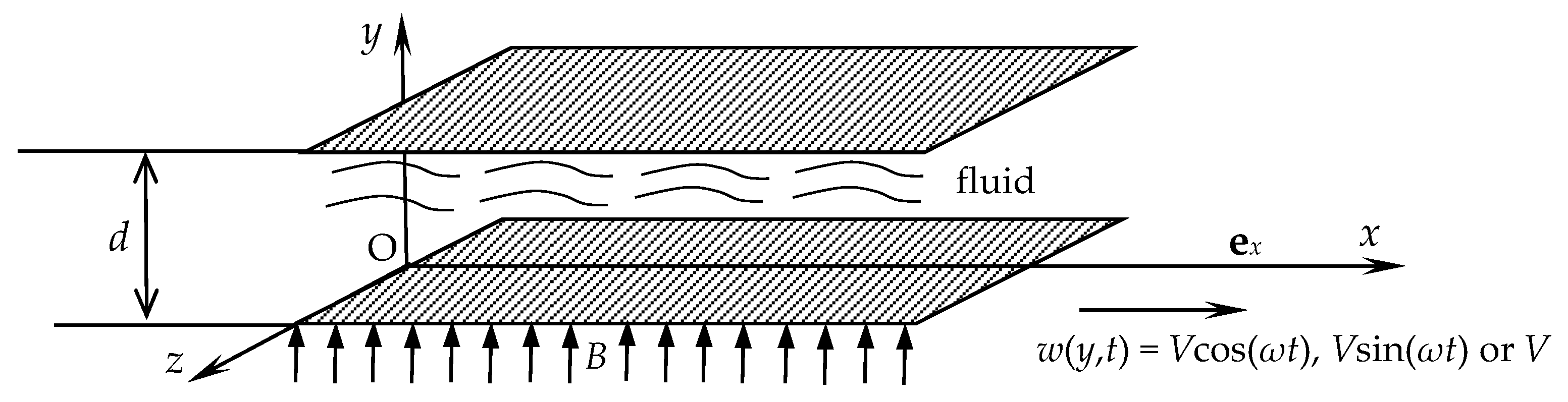
2. Problem Presentation

Let us suppose that an electrically conducting incompressible viscous fluid with exponential dependence of viscosity on pressure is stationary between two unbounded horizontal parallel flat plates, as illustrated in Figure 1.

The constitutive equations of such a fluid are given by the following relations [14,19,22]:

$$\mathit{T}=-p\mathit{I}+\mathit{S}, \mathit{S}=\eta (p)(\mathit{L}+{\mathit{L}}^T), \eta (p)=\mu {\mathrm{e}}^{\alpha (p-p_0)}.$$

(1)

In the above relations, T is the stress tensor; S is the extra-stress tensor; I is the unit tensor; $\mathit{L}=gradw$, where w is the velocity vector; p is the hydrostatic pressure; $\mu$ is the fluid viscosity at the reference pressure $p_0$; and $\alpha >0$ is the dimensional pressure viscosity coefficient. If $\alpha \to 0$ and $\eta (p)\to \mu$, the governing Equation (1) corresponds to incompressible viscous fluids. The fact that $\eta (p)\to \infty$ when pressure $p\to \infty$ has been experimentally confirmed.

The balance of linear momentum for MHD unsteady motions of incompressible fluids leads to the following differential equation [33]:

$$\rho {\displaystyle \frac{\partial w}{\partial t}}=-\nabla p+\mathrm{div}\mathit{S}+{\mathit{F}}_e, {\mathit{F}}_e={\rho }_e\mathit{E}+\mathit{j}\times \mathit{B},$$

(2)

where $\rho$ is the fluid density, w is the velocity vector, and ${\mathit{F}}_e$ is the force arising from the excess charge density ${\rho }_e$ and the induced magnetic effect. The first term of ${\mathit{F}}_e$ is the electrostatic force on the excess charge due to the imposed electric field E; the second term represents the force due to the interaction between the electric current j and the magnetic induction B.

We assume that, at the moment $t=0^{+}$, the lower plate begins to oscillate in its plane with velocity $V\cos (\omega t)$ or $V\sin (\omega t)$, or begins to slide in the same plane with constant velocity V. Here, $\omega$ is the oscillation frequency, and the respective motions correspond to the modified Stokes problems [19], which have multiple engineering applications. A magnetic field of constant strength B acts orthogonally to the plates. Owing to the shear, the fluid begins to move. Because both plates are unbounded, following Rajagopal et al. [19], we now seek the velocity vector w and the hydrostatic pressure p, in a convenient Cartesian coordinate system x, y, and z, in the following form:

$$\mathit{w}=\mathit{w}(y,t)=w(y,t){\mathbf{e}}_x, p=p(y); 0<y<d, t>0,$$

(3)

where ${\mathbf{e}}_x$ is the unit vector along the x-axis of the chosen coordinate system, and d is the distance between plates. The continuity equation for such motions is satisfied. Introducing the velocity vector $\mathit{w}(y,t)$ from Equation (3) into (1), it is found that the non-null component $\tau (y,t)=S_{xy}(y,t)$ of the extra-stress tensor S is given by the relation

$$\tau (y,t)=\mu {\mathrm{e}}^{\alpha (p-p_0)}{\displaystyle \frac{\partial w(y,t)}{\partial y}}; 0<y<d, t>0.$$

(4)

We also suppose the following: that the fluid is finitely conducting; that the induced magnetic field is small enough in comparison with the applied magnetic field and can be neglected; that the magnetic permeability of the fluid is constant; and that there is no electric charge distribution in the fluid. Under these conditions, the balance of linear momentum (2) may be reduced to the following relevant differential equations [33]:

$$\rho {\displaystyle \frac{\partial w(y,t)}{\partial t}}={\displaystyle \frac{\partial \tau (y,t)}{\partial y}}-\sigma B^{2}w(y,t); {\displaystyle \frac{dp(y)}{dy}}=-\rho g; 0<y<d, t>0,$$

(5)

where $\sigma$ is the electric conductivity of the fluid, and g is the gravitational acceleration. From the second equality (5), it follows that

$$p(y)=\rho g(d-y)+p_0 \mathrm{where} p_0=p(d).$$

(6)

Substituting $p(y)$ from Equation (6) into (4), one finds that

$$\tau (y,t)=\mu {\mathrm{e}}^{\alpha \rho g(d-y)}{\displaystyle \frac{\partial w(y,t)}{\partial y}}; 0<y<d, t>0.$$

(7)

The initial and boundary conditions for the modified second problem of Stokes are

$$w(y,0)=0; 0\le y\le d,$$

(8)

$$w(0,t)=V\cos (\omega t) \mathrm{or} V\sin (\omega t), w(d,t)=0; t>0.$$

(9)

The dimensionless forms of the governing Equations (5) and (7), namely,

$${\displaystyle \frac{\partial w(y,t)}{\partial t}}={\displaystyle \frac{\partial \tau (y,t)}{\partial y}}-Mw(y,t); 0<y<1, t>0,$$

(10)

$$\tau (y,t)={\displaystyle \frac{1}{\mathrm{Re}}}{\mathrm{e}}^{\alpha (1-y)}{\displaystyle \frac{\partial w(y,t)}{\partial y}}; 0<y<1, t>0,$$

(11)

are now obtained using the following non-dimensional functions, variables, and parameters:

$$w^{\ast }={\displaystyle \frac{1}{V}}w, {\tau }^{\ast }={\displaystyle \frac{1}{\rho V^2}}\tau , y^{\ast }={\displaystyle \frac{1}{d}}y, t^{\ast }={\displaystyle \frac{V}{d}}t, {\alpha }^{\ast }=\alpha \rho gd,$$

(12)

The star notation in the above is ignored. In the last equalities, the magnetic parameter M and the Reynolds number Re are defined by the following relations:

$$M={\displaystyle \frac{\sigma B^2}{\rho }}{\displaystyle \frac{d}{V}}, \mathrm{Re}={\displaystyle \frac{Vd}{\nu }},$$

(13)

where $\nu =\mu /\rho$ is the kinematic viscosity of the fluid. By replacing $\tau (y,t)$ in Equation (11) with (10), the following governing equation is obtained for the non-dimensional velocity field $w(y,t)$:

$${\displaystyle \frac{\partial w(y,t)}{\partial t}}={\displaystyle \frac{1}{\mathrm{Re}}}{\mathrm{e}}^{\alpha (1-y)}\left[{\displaystyle \frac{{\partial }^{2}w(y,t)}{\partial y^2}}-\alpha {\displaystyle \frac{\partial w(y,t)}{\partial y}}\right]-Mw(y,t); 0<y<1, t>0,$$

(14)

The non-dimensional forms of the initial and boundary conditions (8) and (9) are as follows:

$$w(y,0)=0; 0\le y\le 1.$$

(15)

$$w(0,t)=\cos (\omega t) \mathrm{or} \sin (\omega t), w(1,t)=0; t>0,$$

(16)

where the new $\omega$ is the dimensionless frequency of the oscillations.

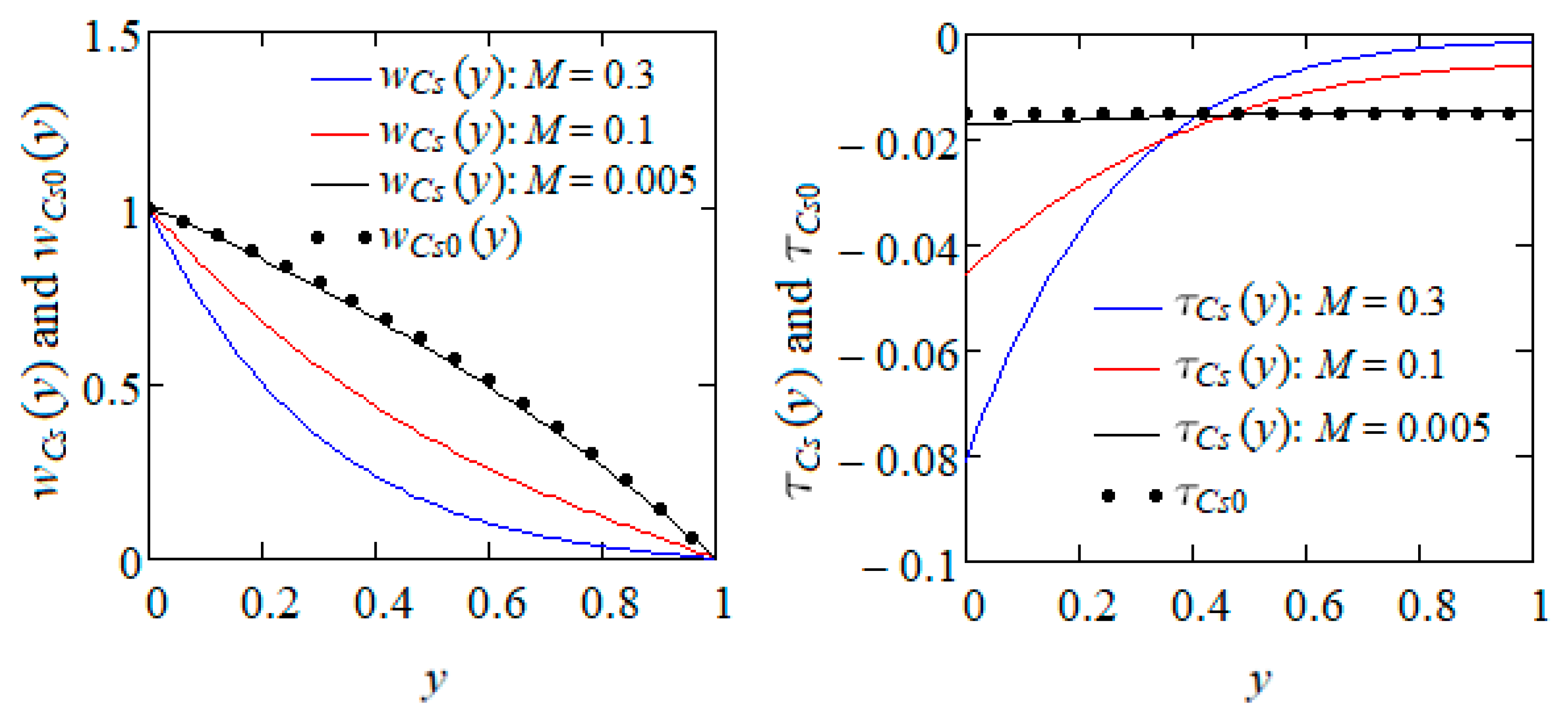
3. Steady-State Solutions for the Modified Stokes Problems

Next, to avoid confusion, let us denote by $w_c(y,t)$ and $w_s(y,t)$ the start-up velocities corresponding to motions induced by cosine and sine oscillations, respectively, of the lower plate. Because the respective motions become steady in time, their start-up velocity fields $w_c(y,t)$ and $w_s(y,t)$ can be presented as sums of their steady-state (long-time) and transient components, as follows:

$$\begin{array}{l}{w}_c(y,t)=w_{cs}(y,t)+w_{ct}(y,t),\\ w_s(y,t)=w_{ss}(y,t)+w_{st}(y,t); 0<y<1, t>0.\end{array}$$

(17)

For some time after motion initiation, the fluid moves according to the start-up velocities $w_c(y,t)$ and $w_s(y,t)$. This is the time taken to reach the steady state. After this time, the fluid motion is characterized by the steady-state components $w_{cs}(y,t)$ and $w_{ss}(y,t)$ of these velocities. It is well known that these components, also called steady-state solutions, are independent of the initial conditions but satisfy the governing Equation (14) and the boundary conditions (16).

In practice, the time required to reach the steady state is very important for experimental researchers. To determine this time, it is necessary and sufficient to know the steady-state velocities. Consequently, in the following section, we shall first derive analytical expressions for $w_{cs}(y,t)$ and $w_{ss}(y,t)$. To determine these expressions at the same time, we use the complex velocity

$$w_{com}(y,t)=w_{cs}(y,t)+i{w}_{ss}(y,t); 0<y<1, t>0,$$

(18)

which has to satisfy the partial differential equation

$${\displaystyle \frac{\partial w_{com}(y,t)}{\partial t}}={\displaystyle \frac{1}{\mathrm{Re}}}{\mathrm{e}}^{\alpha (1-y)}\left[{\displaystyle \frac{{\partial }^2{w}_{com}(y,t)}{\partial y^2}}-\alpha {\displaystyle \frac{\partial w_{com}(y,t)}{\partial y}}\right]-M{w}_{com}(y,t); 0<y<1, t>0,$$

(19)

and the boundary conditions

$$w_{com}(0,t)={\mathrm{e}}^{i\omega t}, w_{com}(1,t)=0; t>0.$$

(20)

In Equation (18), i is the imaginary unit.

Changing the independent variable $y=1+\ln \sqrt[\alpha ]{r}$ in Equation (19), one finds that $w_{com}(r,t)$ has to satisfy the next boundary value problem:

$${\displaystyle \frac{\partial w_{com}(r,t)}{\partial t}}={\displaystyle \frac{r{\alpha }^2}{\mathrm{Re}}}{\displaystyle \frac{{\partial }^2{w}_{com}(r,t)}{\partial r^2}}-M{w}_{com}(r,t); {\displaystyle \frac{1}{{\mathrm{e}}^{\alpha }}}<r<1, t>0,$$

(21)

$$w_{com}\left({\displaystyle \frac{1}{{\mathrm{e}}^{\alpha }}},t\right)={\mathrm{e}}^{i\omega t}, w_{com}(1,t)=0; {\displaystyle \frac{1}{{\mathrm{e}}^{\alpha }}}<r<1, t>0.$$

(22)

Bearing in mind the homogeneity of the governing Equation (21), and the form of the boundary conditions (22), we now seek a solution of the form

$$w_{com}(r,t)=W(r){\mathrm{e}}^{i\omega t}; {\displaystyle \frac{1}{{\mathrm{e}}^{\alpha }}}<r<1, t>0,$$

(23)

in which the complex function $W(\cdot )$ has to be determined.

Replacing the complex velocity $w_{com}(r,t)$ from Equation (23) in (21), and bearing in mind the boundary conditions (22), it follows that the unknown function $W(r)$ has to satisfy the boundary value problem

$$r{\displaystyle \frac{d^{2}W(r)}{d{r}^2}}+\beta W(r)=0; W\left({\displaystyle \frac{1}{{\mathrm{e}}^{\alpha }}}\right)=1, W(1)=0,$$

(24)

where $\beta =-(M+i\omega )\mathrm{Re}/{\alpha }^2$.

Now, applying the observation (see [34], exercise 37 on page 251) that “The general solution of the ordinary differential equation $x{y}^{″}+\lambda y=0$ is

$$y=\sqrt{x}[c_1{J}_1(2\sqrt{\lambda x})+c_2{Y}_1(2\sqrt{\lambda x})]\hspace{0.17em},$$

(25)

where $J_1(\cdot )$ and $Y_1(\cdot )$ are Bessel functions of the first and second kind of one order”, it is not difficult to show that

$$W(r)=\sqrt{r{\mathrm{e}}^{\alpha }}{\displaystyle \frac{Y_1(2\sqrt{\beta })J_1(2\sqrt{\beta r})-J_1(2\sqrt{\beta })Y_1(2\sqrt{\beta r})}{Y_1(2\sqrt{\beta })J_1(2\sqrt{\beta /{\mathrm{e}}^{\alpha }})-J_1(2\sqrt{\beta })Y_1(2\sqrt{\beta /{\mathrm{e}}^{\alpha }})}}; {\displaystyle \frac{1}{{\mathrm{e}}^{\alpha }}}<r<1.$$

(26)

In conclusion, bearing in mind relations (18), (23), and (26), and the change of the independent variable that has been previously used, it follows that the dimensionless steady-state velocities $w_{cs}(y,t)$ and $w_{ss}(y,t)$ are given by the following expressions:

$$w_{cs}(y,t)=\sqrt{{\mathrm{e}}^{\alpha y}}\Re \mathrm{e}\left\{{\displaystyle \frac{Y_1(2\sqrt{\beta })J_1(2\sqrt{\beta {\mathrm{e}}^{\alpha (y-1)}})-J_1(2\sqrt{\beta })Y_1(2\sqrt{\beta {\mathrm{e}}^{\alpha (y-1)}})}{Y_1(2\sqrt{\beta })J_1(2\sqrt{\beta /{\mathrm{e}}^{\alpha }})-J_1(2\sqrt{\beta })Y_1(2\sqrt{\beta /{\mathrm{e}}^{\alpha }})}}{\mathrm{e}}^{i\omega t}\right\},$$

(27)

$$w_{ss}(y,t)=\sqrt{{\mathrm{e}}^{\alpha y}}\mathrm{Im}\left\{{\displaystyle \frac{Y_1(2\sqrt{\beta })J_1(2\sqrt{\beta {\mathrm{e}}^{\alpha (y-1)}})-J_1(2\sqrt{\beta })Y_1(2\sqrt{\beta {\mathrm{e}}^{\alpha (y-1)}})}{Y_1(2\sqrt{\beta })J_1(2\sqrt{\beta /{\mathrm{e}}^{\alpha }})-J_1(2\sqrt{\beta })Y_1(2\sqrt{\beta /{\mathrm{e}}^{\alpha }})}}{\mathrm{e}}^{i\omega t}\right\},$$

(28)

where $\Re \mathrm{e}$ and Im denote the real and imaginary parts, respectively, of that which follows. Making M = 0 in the last two equalities, the dimensionless steady-state velocity fields obtained by Rauf et al. [35] are recovered, as expected.

The corresponding expressions of the dimensionless steady-state shear stresses ${\tau }_{cs}(y,t)$ and ${\tau }_{ss}(y,t)$ which correspond to the two motion problems, namely,

$${\tau }_{cs}(y,t)=\sqrt{{\displaystyle \frac{{\mathrm{e}}^{\alpha }}{\mathrm{Re}}}}\Re \mathrm{e}\left\{{\displaystyle \frac{Y_1(2\sqrt{\beta })J_0(2\sqrt{\beta {\mathrm{e}}^{\alpha (y-1)}})-J_1(2\sqrt{\beta })Y_0(2\sqrt{\beta {\mathrm{e}}^{\alpha (y-1)}})}{Y_1(2\sqrt{\beta })J_1(2\sqrt{\beta /{\mathrm{e}}^{\alpha }})-J_1(2\sqrt{\beta })Y_1(2\sqrt{\beta /{\mathrm{e}}^{\alpha }})}}\sqrt{i\omega +M }{\mathrm{e}}^{i(\omega t+\pi /2)}\right\},$$

(29)

$${\tau }_{ss}(y,t)=\sqrt{{\displaystyle \frac{{\mathrm{e}}^{\alpha }}{\mathrm{Re}}}}\mathrm{Im}\left\{{\displaystyle \frac{Y_1(2\sqrt{\beta })J_0(2\sqrt{\beta {\mathrm{e}}^{\alpha (y-1)}})-J_1(2\sqrt{\beta })Y_0(2\sqrt{\beta {\mathrm{e}}^{\alpha (y-1)}})}{Y_1(2\sqrt{\beta })J_1(2\sqrt{\beta /{\mathrm{e}}^{\alpha }})-J_1(2\sqrt{\beta })Y_1(2\sqrt{\beta /{\mathrm{e}}^{\alpha }})}}\sqrt{i\omega +M }{\mathrm{e}}^{i(\omega t+\pi /2)}\right\},$$

(30)

are obtained by substituting $w_{cs}(y,t)$ and $w_{ss}(y,t)$ from relations (27) and (28) into (11), and using the known identity ${J^{\prime }}_1(z)=J_0(z)-J_1(z)/z$. Direct computations show that the expressions of $w_{cs}(y,t)$, $w_{ss}(y,t)$, ${\tau }_{cs}(y,t)$, and ${\tau }_{ss}(y,t)$ given by relations (27)–(30) satisfy the imposed boundary conditions and the corresponding governing equations. Taking $M=0$ in the above relations, solutions are obtained which correspond to the same motions of incompressible viscous fluids whose viscosity depends exponentially on pressure, but in the absence of a magnetic field.

3.1. Limiting Case $\alpha \to 0$ (MHD Modified Stokes Second Problem for Ordinary Fluids)

On the basis of the asymptotic approximations

$$J_{\nu }(z)\approx \sqrt{{\displaystyle \frac{2}{\pi z}}}\cos \left[z-{\displaystyle \frac{(2\nu +1)\pi }{4}}\right], Y_{\nu }(z)\approx \sqrt{{\displaystyle \frac{2}{\pi z}}}\sin \left[z-{\displaystyle \frac{(2\nu +1)\pi }{4}}\right] \mathrm{for} \left|z\right|>>1,$$

(31)

which, in our case, are valid when $\alpha$ is sufficiently small and $\left|\beta \right|>>1$, we can show that

$$w_{cs}(y,t)\approx \sqrt[4]{{\mathrm{e}}^{\alpha y}}\Re \mathrm{e}\left\{{\displaystyle \frac{\sin \left\{2\sqrt{\beta }\left[1-\exp \left(\frac{\alpha (\mathrm{y}-1)}{2}\right)\right]\right\}}{\sin \left\{2\sqrt{\beta }\left[1-\exp \left(-\frac{\alpha }{2}\right)\right]\right\}}}{\mathrm{e}}^{i\omega t}\right\} ; 0<y<1, t>0,$$

(32)

$$w_{ss}(y,t)\approx \sqrt[4]{{\mathrm{e}}^{\alpha y}}\mathrm{Im}\left\{{\displaystyle \frac{\sin \left\{2\sqrt{\beta }\left[1-\exp \left(\frac{\alpha (\mathrm{y}-1)}{2}\right)\right]\right\}}{\sin \left\{2\sqrt{\beta }\left[1-\exp \left(-\frac{\alpha }{2}\right)\right]\right\}}}{\mathrm{e}}^{i\omega t}\right\} ; 0<y<1, t>0.$$

(33)

Developing in Maclaurin series the functions $\exp [\alpha (y-1)/2]$ and $\exp (-\alpha /2)$ from equalities (32) and (33), and taking the limits of the resulting expressions, one obtains the dimensionless steady-state velocities

$$w_{Ocs}(y,t)=\Re \mathrm{e}\left\{{\displaystyle \frac{\sin \mathrm{h}\left[\right(1-y)\sqrt{(i\omega +M)\mathrm{Re}}]}{\sin \mathrm{h}[\sqrt{(i\omega +M)\mathrm{Re}}]}}{\mathrm{e}}^{i\omega t}\right\}\hspace{0.17em}; 0<y<1, t>0,$$

(34)

$$w_{Oss}(y,t)=\mathrm{Im}\left\{{\displaystyle \frac{\sin \mathrm{h}\left[\right(1-y)\sqrt{(i\omega +M)\mathrm{Re}}]}{\sin \mathrm{h}[\sqrt{(i\omega +M)\mathrm{Re}}]}}{\mathrm{e}}^{i\omega t}\right\} ; 0<y<1, t>0,$$

(35)

corresponding to the MHD modified second problem of Stokes for ordinary viscous fluids. In order to write them in the present form, we also used the fact that $\sin (iz)=i\sinh (z)$. Taking $M=0$ in Equations (34) and (35), one recovers the expressions of the dimensionless steady-state velocities obtained by Fetecau and Narahary [36], Equation (49), using a different method, namely

$$\begin{array}{l}{w}_{Ocs}(y,t)=\Re \mathrm{e}\left\{{\displaystyle \frac{\sin \mathrm{h}\left[\right(1-y)\sqrt{i\omega \mathrm{Re}}]}{\sin \mathrm{h}(\sqrt{i\omega \mathrm{Re}})}}{\mathrm{e}}^{i\omega t}\right\}\hspace{0.17em};\\ w_{Ocs}(y,t)=\Re \mathrm{e}\left\{{\displaystyle \frac{\sin \mathrm{h}\left[\right(1-y)\sqrt{i\omega \mathrm{Re}}]}{\sin \mathrm{h}(\sqrt{i\omega \mathrm{Re}})}}{\mathrm{e}}^{i\omega t}\right\}.\end{array}$$

The corresponding steady-state shear stresses obtained by introducing $w_{Ocs}(y,t)$ and $w_{Oss}(y,t)$ in Equation (11) have the expressions

$${\tau }_{Ocs}(y,t)=-{\displaystyle \frac{1}{\sqrt{\mathrm{Re}}}}\Re \mathrm{e}\left\{\sqrt{i\omega +M}{\displaystyle \frac{\cos \mathrm{h}\left[\right(1-y)\sqrt{(i\omega +M)\mathrm{Re}}]}{\sin \mathrm{h}[\sqrt{(i\omega +M)\mathrm{Re}}]}}{\mathrm{e}}^{i\omega t}\right\} ; 0<y<1, t>0,$$

(36)

$${\tau }_{Oss}(y,t)=-{\displaystyle \frac{1}{\sqrt{\mathrm{Re}}}}\mathrm{Im}\left\{\sqrt{i\omega +M}{\displaystyle \frac{\cos \mathrm{h}\left[\right(1-y)\sqrt{(i\omega +M)\mathrm{Re}}]}{\sin \mathrm{h}[\sqrt{(i\omega +M)\mathrm{Re}}]}}{\mathrm{e}}^{i\omega t}\right\}\hspace{0.17em}; 0<y<1, t>0.$$

(37)

3.2. Case Study $\omega =0$ (MHD Modified Stokes First Problem)

The dimensionless start-up velocity and the adequate shear stress corresponding to this motion of fluids with exponential dependence of viscosity on pressure shall be denoted by $w_C(y,t)$ and ${\tau }_C(y,t)$. These correspond to the MHD motion of incompressible viscous fluids with exponential dependence of viscosity on pressure induced by the lower plate that slides in its plane with constant velocity V; this can also be expressed as the sum of their steady and transient components, as follows:

$$w_C(y,t)=w_{Cs}(y,t)\hspace{0.17em}+w_{Ct}(y,t), {\tau }_C(y,t)={\tau }_{Cs}(y,t)\hspace{0.17em}+{\tau }_{Ct}(y,t); 0<y<1, t>0.$$

(38)

Taking $\omega =0$ in Equations (27) and (29), one finds the dimensionless steady velocity $w_{Cs}(y)$ and the shear stress ${\tau }_{Cs}(y)$ corresponding to this motion. Their expressions are given by the relations

$$w_{Cs}(y)=\sqrt{{\mathrm{e}}^{\alpha y}}\Re \mathrm{e}\left\{{\displaystyle \frac{Y_1(2\sqrt{\gamma })J_1(2\sqrt{\gamma {\mathrm{e}}^{\alpha (y-1)}})-J_1(2\sqrt{\gamma })Y_1(2\sqrt{\gamma {\mathrm{e}}^{\alpha (y-1)}})}{Y_1(2\sqrt{\gamma })J_1(2\sqrt{\gamma /{\mathrm{e}}^{\alpha }})-J_1(2\sqrt{\gamma })Y_1(2\sqrt{\gamma /{\mathrm{e}}^{\alpha }})}}\right\}; 0<y<1,$$

(39)

$${\tau }_{Cs}(y)=\sqrt{{\displaystyle \frac{M{\mathrm{e}}^{\alpha }}{\mathrm{Re}}}}\Re \mathrm{e}\left\{{\displaystyle \frac{Y_1(2\sqrt{\gamma })J_0(2\sqrt{\gamma {\mathrm{e}}^{\alpha (y-1)}})-J_1(2\sqrt{\gamma })Y_0(2\sqrt{\gamma {\mathrm{e}}^{\alpha (y-1)}})}{Y_1(2\sqrt{\gamma })J_1(2\sqrt{\gamma /{\mathrm{e}}^{\alpha }})-J_1(2\sqrt{\gamma })Y_1(2\sqrt{\gamma /{\mathrm{e}}^{\alpha }})}}{\mathrm{e}}^{i\pi /2}\right\}; 0<y<1,$$

(40)

where $\gamma =-M\mathrm{Re}/{\alpha }^2$.

Finally, using the asymptotic approximations

$$J_0(z)\approx 1, J_1(z)\approx {\displaystyle \frac{z}{2}}, Y_0(z)\approx {\displaystyle \frac{2}{\pi }}\left[\ln \left({\displaystyle \frac{z}{2}}\right)+\delta \right]\hspace{0.17em}, Y_1(z)\approx -{\displaystyle \frac{2\pi }{z}} \mathrm{for} \left|z\right|\hspace{0.17em}<<1,$$

(41)

for the Bessel functions from Equations (39) and (40), and taking the limits of the respective relations when $M\to 0$, we recover the expressions

$$\underset{M\to 0}{\lim }{w}_{Cs}(y)={\displaystyle \frac{{\mathrm{e}}^{\alpha y}-{\mathrm{e}}^{\alpha }}{1-{\mathrm{e}}^{\alpha }}}=w_{Cs0}(y), \underset{M\to 0}{\lim }{\tau }_{Cs}(y)={\displaystyle \frac{\alpha {\mathrm{e}}^{\alpha }}{(1-{\mathrm{e}}^{\alpha })\mathrm{Re}}}={\tau }_{Cs0}; 0<y<1,$$

(42)

obtained by Fetecau et al. [22], Equation (64), using a different technique. These expressions can also be directly determined by solving the corresponding boundary value problems. In the penultimate approximation from relation (41), $\delta =0.5772$ is the Euler–Mascheroni constant. Finally, for certainty, the convergence of the steady velocity $w_{Cs}(y)$ and of the shear stress ${\tau }_{Cs}(y)$ to $w_{Cs0}(y)$ and ${\tau }_{Cs0}$, respectively, is also graphically shown in Figure 2 for decreasing values of the magnetic parameter M.

From the relations expressed in (42), it clearly follows that the steady shear stress corresponding to the first problem of Stokes for incompressible viscous fluids with exponential dependence of viscosity on pressure is constant for the entire flow domain, although the corresponding velocity of the fluid is a function of the spatial variable y. Furthermore, taking the limits of the expressions of equality (42) when the parameter $\alpha \to 0$, the non-dimensional steady velocity and shear stress fields

$$w_{OCs}(y)=1-y, {\tau }_{OCs}=-{\displaystyle \frac{1}{\mathrm{Re}}},$$

(43)

corresponding to the simple Couette flow of incompressible viscous fluids are recovered.

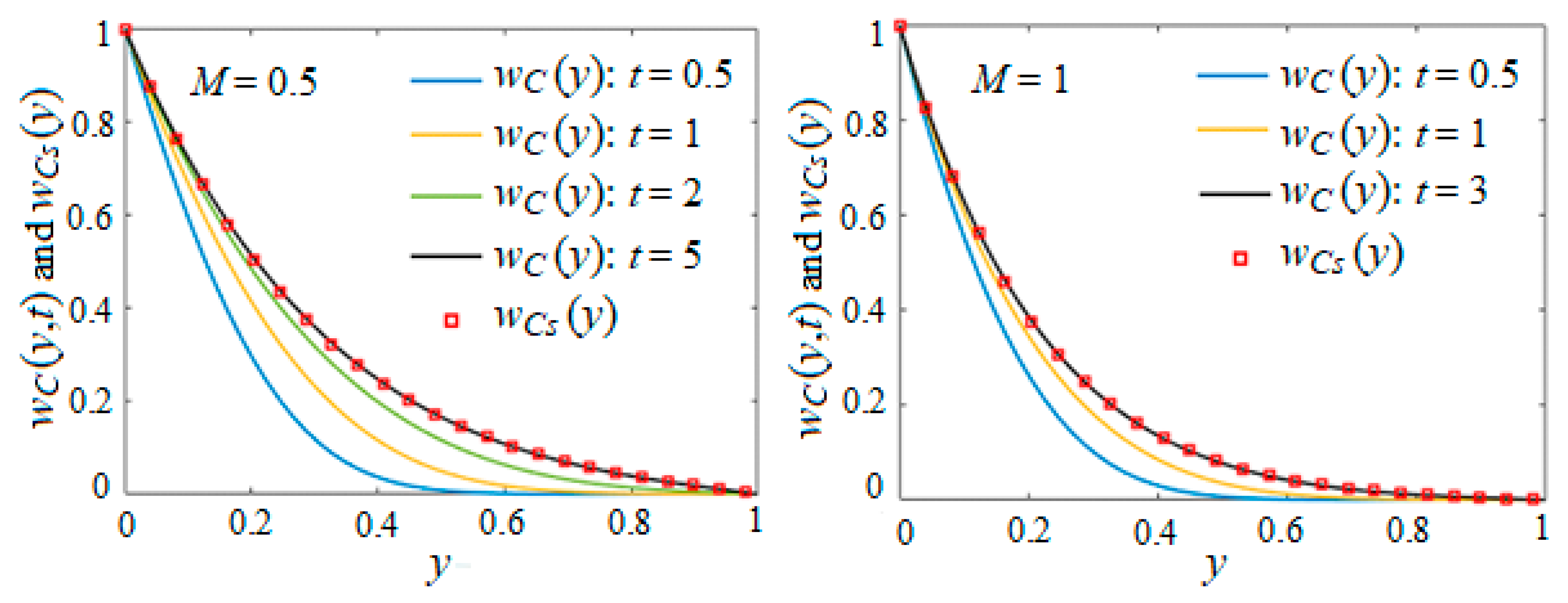
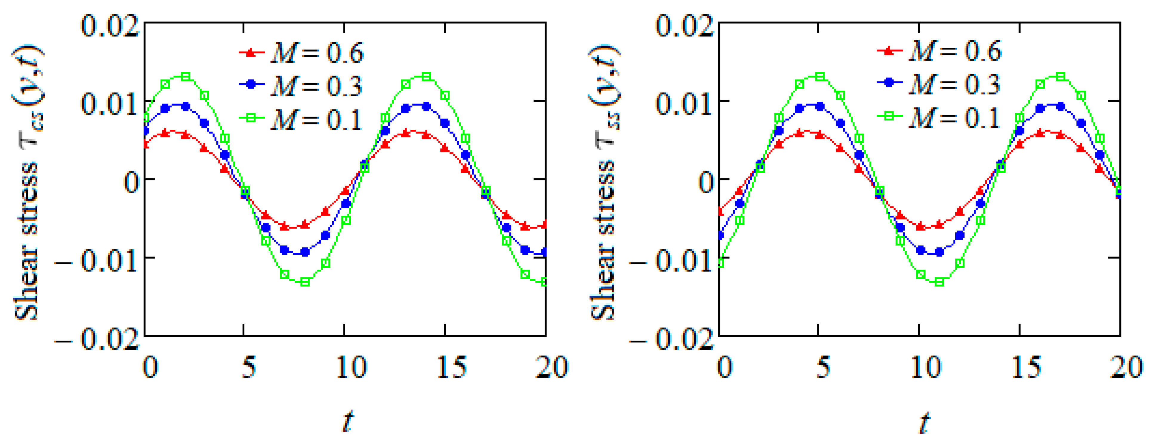
4. Numerical Results and Conclusions

In this study, modified Stokes problems involving incompressible viscous fluids whose viscosity depends exponentially on pressure were analytically and numerically investigated, with magnetic effects and gravitational acceleration also being taken into account. Exact analytical expressions were derived for the dimensionless steady-state velocity fields and the adequate shear stresses. As expected, some of their particularizations reduced to known results from the literature. In addition, to check the general solutions and obtain some characteristic features of the fluid behavior, as illustrated in Figure 3, we showed that the dimensionless starting velocity $w_C(y,t)$ (numerical solutions, obtained using the finite difference method) converged to its steady component $w_{Cs}(y)$ with increasing values of time t. Moreover, from these figures, it was also easily observed that the time required to reach the steady state and the fluid velocity both declined in the presence of the magnetic field. Indeed, this time declined from a value of 5 to a value of 3 when the value of the magnetic parameter M increased from 0.5 to 1. A careful analysis of these graphical representations also showed that the fluid velocity slowly decreased when M increased from 0.5 to 1. In addition, and as expected, the fluid velocity increased with increasing values of time t.

Figure 4 and Figure 5 present variations in time of the dimensionless steady-state velocity fields $w_{cs}(y,t),$ $w_{ss}(y,t)$ and of the corresponding shear stresses ${\tau }_{cs}(y,t)$ and ${\tau }_{ss}(y,t)$ in the middle of the channel for decreasing values of the magnetic parameter M and fixed values of the other physical parameters.

The oscillatory character of these entities and the phase difference between the two motions induced by cosine or sine oscillations of the lower plate are clearly visualized. In addition, the oscillations’ amplitudes, which are the same for both motions at equal values of parameters, decline with increasing values of M. As expected, this result shows that the fluid velocity declines with increasing values of M, in accordance with the findings illustrated in Figure 3.

The main results of the present study may now be stated, as follows:

• Modified Stokes problems involving incompressible viscous fluids whose viscosity depends exponentially on pressure were studied analytically and numerically, with magnetic effects and gravitational acceleration also being taken into account.
• Exact expressions were derived for the dimensionless steady-state velocity fields and the associated shear stresses. The fluid velocity $w_{Cs}(y)$ was utilized, as shown in Figure 3, to calculate the time required to reach the steady state, a critical parameter for experimental researchers.
• Graphical analysis clearly revealed that the fluid achieved steady-state motion later, and flowed more quickly, when the magnetic field was absent. As expected, some known results from the literature were recovered as limiting cases of the present solutions.
• The oscillatory character of the velocity fields $w_{cs}(y,t)$ and $w_{ss}(y,t)$ and of the corresponding shear stresses, as well as their evolution at distinct values of the magnetic parameter M, was underlined, as shown in Figure 4 and Figure 5. As expected, the oscillations’ amplitudes decline with increasing values of M.

References

1. Renardy, M. Parallel shear flows of fluids with a pressure dependent viscosity. J. Non-Newton. Fluid Mech. 2003, 114, 229–236. [Google Scholar] [CrossRef]
2. Denn, M.M. Polymer Melt Processing; Cambridge University Press: Cambridge, UK, 2008. [Google Scholar]
3. Rajagopal, K.R.; Saccomandi, G.; Vergori, L. Flow of fluids with pressure and shear-dependent viscosity down an inclined plane. J. Fluid Mech. 2003, 706, 173–189. [Google Scholar] [CrossRef]
4. Le Roux, C. Flow of fluids with pressure dependent viscosities in an orthogonal rheometer subject to slip boundary conditions. Meccanica 2009, 44, 71–83. [Google Scholar] [CrossRef]
5. Martinez-Boza, F.J.; Martin-Alfonso, M.J.; Callegas, C.; Fernandez, M. High-pressure behavior of intermediate fuel oils. Energy Fuels 2011, 25, 5138–5144. [Google Scholar] [CrossRef]
6. Dealy, J.M.; Wang, J. Melt Rheology and Its Applications in the Plastic Industry, 2nd ed.; Springer: Dordrecht, The Netherlands, 2013. [Google Scholar]
7. Andrade, C. Viscosity of liquids. Nature 1930, 125, 309–310. [Google Scholar] [CrossRef]
8. Bridgman, P.W. The Physics of High Pressure; MacMillan Company: New York, NY, USA, 1931. [Google Scholar]
9. Griest, E.M.; Webb, W.; Schiessler, R.W. Effect of pressure on viscosity of high hydrocarbons and their mixture. J. Chem. Phys. 1958, 29, 711–720. [Google Scholar] [CrossRef]
10. Johnson, K.L.; Cameron, R. Shear behavior of elastohydrodynamic oil films at high rolling contact pressures. Proc. Inst. Mech. Eng. 1967, 182, 307–330. [Google Scholar] [CrossRef]
11. Johnson, K.L.; Greenwood, J.A. Thermal analysis of an Eyring fluid in elastohydrodynamic traction. Wear 1980, 61, 355–374. [Google Scholar] [CrossRef]
12. Bair, S.; Winer, W.O. The high pressure high shear stress rheology of liquid lubricants. J. Tribol. 1992, 114, 1–9. [Google Scholar] [CrossRef]
13. Hron, J.; Malek, J.; Rajagopal, K.R. Simple flows of fluids with pressure dependent viscosities. Proc. Roy. Soc. Lond. Ser. A Math. Phys. Eng. Sci. 2001, 457, 1603–1622. [Google Scholar] [CrossRef]
14. Rajagopal, K.R. Couette flows of fluids with pressure dependent viscosity. Int. J. Appl. Mech. Eng. 2004, 9, 573–585. [Google Scholar]
15. Rajagopal, K.R. A semi-inverse problem of flows of fluids with pressure-dependent viscosities. Inverse Probl. Sci. Eng. 2008, 16, 269–280. [Google Scholar] [CrossRef]
16. Prusa, V. Revisiting Stokes first and second problems for fluids with pressure-dependent viscosities. Int. J. Eng. Sci. 2010, 48, 2054–2065. [Google Scholar] [CrossRef]
17. Akyildiz, F.T.; Siginer, D. A note on the steady flow of Newtonian fluids with pressure dependent viscosity in a rectangular duct. Int. J. Eng. Sci. 2016, 104, 1–4. [Google Scholar] [CrossRef]
18. Housiadas, K.D.; Georgiou, G.C. Analytical solution of the flow of a Newtonian fluid with pressure-dependent viscosity in a rectangular duct. Appl. Math. Comput. 2018, 322, 123–128. [Google Scholar] [CrossRef]
19. Rajagopal, K.R.; Saccomandi, G.; Vergori, L. Unsteady flows of fluids with pressure dependent viscosity. J. Math. Anal. Appl. 2013, 404, 362–372. [Google Scholar] [CrossRef]
20. Fetecau, C.; Vieru, D. Exact solutions for unsteady motion between parallel plates of some fluids with power-law dependence of viscosity on the pressure. Appl. Eng. Sci. 2020, 1, 100003. [Google Scholar] [CrossRef]
21. Fetecau, C.; Bridges, C. Analytical solutions for some unsteady flows of fluids with linear dependence of viscosity on the pressure. Inverse Probl. Sci. Eng. 2021, 29, 378–395. [Google Scholar] [CrossRef]
22. Fetecau, C.; Rauf, A.; Qureshi, T.M.; Mahmood, O.U. Analytical solutions of upper-convected Maxwell fluid flow with exponential dependence of viscosity on the pressure. Eur. J. Mech. B Fluids 2021, 88, 148–159. [Google Scholar] [CrossRef]
23. Srinivasan, S.; Rajagopal, K.R. A note on the flow of a fluid with pressure-dependent viscosity in the annulus of two infinite long coaxial cylinders. Appl. Math. Model. 2010, 34, 3255–3263. [Google Scholar] [CrossRef]
24. Kalogirou, A.; Poyiadji, S.; Georgiou, G.C. Incompressible Poiseuille flows of Newtonian liquids with a pressure-dependent viscosity. J. Non-Newton. Fluid Mech. 2011, 166, 413–419. [Google Scholar] [CrossRef]
25. Housiadas, K.D.; Georgiou, G.C.; Tanner, R.I. A note on the unbounded creeping flow past a sphere for Newtonian fluids with pressure-dependent viscosity. Int. J. Eng. Sci. 2015, 86, 1–9. [Google Scholar] [CrossRef]
26. Zehra, I.; Kousar, N.; Ur Rehman, K. Pressure dependent viscosity subject to Poiseuille and Couette flows via tangent hyperbolic model. Phys. A Stat. Mech. Appl. 2019, 527, 121332. [Google Scholar] [CrossRef]
27. Jia-Bin, W.; Li, L. Pressure-flow rate relationship and its polynomial expansion for laminar flow in a circular pipe based on exponential viscosity-pressure characteristics: An extension of classical Poiseuille’ s law. Phys. Fluids 2023, 35, 103613. [Google Scholar] [CrossRef]
28. Schmelzer, J.W.P.; Abyzov, A.S. Pressure dependence of viscosity: A new general relation. Interfacial Phenom. Heat Transf. 2017, 5, 107–112. [Google Scholar] [CrossRef]
29. Tao, L.N. Magnetohydrodynamic effects on the formation of Couette flow. J. Aerosp. Sci. 1960, 27, 334–338. [Google Scholar] [CrossRef]
30. Katagiri, M. Flow formation in Couette motion in magneto hydrodynamics. Phys. Soc. Jpn. 1962, 17, 393–396. [Google Scholar] [CrossRef]
31. Zahid, M.; Rana, M.A.; Haroom, T.; Siddiqui, A.M. Applications of Sumudu transform to MHD flows of an Oldroyd-B fluid. Appl. Math. Sci. 2013, 7, 7027–7036. [Google Scholar] [CrossRef]
32. Ghosh, A.K.; Datta, S.K.; Sen, P. On hydromagnetic flow of an Oldroyd-B fluid between two oscillating plates. Int. J. Appl. Comput. Math. 2016, 2, 365–386. [Google Scholar] [CrossRef]
33. Rossow, V.J. On flow of electrically conducting fluids over a flat plate in the presence of a transverse magnetic fluid. NACA TN Tech. Rep. 1957, 3971, 489–508. [Google Scholar]
34. Zill, D.G. A First Course in Differential Equations with Modelling Applications, 9th ed.; Brooks/Cole Pub. Co.: Pacific Grove, CA, USA, 2009. [Google Scholar]
35. Rauf, A.; Qureshi, T.M.; Fetecau, C. Analytical and numerical solutions for some motions of viscous fluids with exponential dependence of viscosity on the pressure. Math. Rep. 2023, 25, 465–479. [Google Scholar] [CrossRef]
36. Fetecau, C.; Narahari, M. General solutions for hydromagnetic flow of viscous fluids between horizontal parallel plates through porous medium. J. Eng. Mech. 2020, 146, 04020053. [Google Scholar] [CrossRef]
Figure 1. Geometry of fluid flow.
Axioms 14 00124 g001
Figure 2. Convergence of w C s ( y ) and τ C s ( y ) to w C s 0 ( y ) and τ C s 0 , respectively, when Re = 100 ,   α = 0.9 , and the magnetic parameter M 0 .
Axioms 14 00124 g002
Figure 3. Convergence of velocity w C ( y , t ) (numerical solutions) to its steady component w C s ( y ) given by Equation (39) when α = 0.8 ,   Re = 50 , with increasing values of time t.
Axioms 14 00124 g003
Figure 4. Variations in time of the velocity fields w c s ( y , t ) and w s s ( y , t ) given by Equations (27) and (28) for ω = π / 6 , Re = 100 ,   α = 0.9 ,   y = 0.5 , with decreasing values of M.
Axioms 14 00124 g004
Figure 5. Variations in time of the shear stresses τ c s ( y , t ) and τ s s ( y , t ) given by Equations (29) and (30) for ω = π / 6 ,   Re = 100 ,   α = 0.9 ,   y = 0.5 , with decreasing values of M.
Axioms 14 00124 g005
Disclaimer/Publisher’s Note: The statements, opinions and data contained in all publications are solely those of the individual author(s) and contributor(s) and not of MDPI and/or the editor(s). MDPI and/or the editor(s) disclaim responsibility for any injury to people or property resulting from any ideas, methods, instructions or products referred to in the content.