Abstract
In this article, we are interested in studying and analyzing the heat conduction phenomenon in a multi-layered solid. We consider the physical assumptions that the dual-phase-lag model governs the heat flow on each solid layer. We introduce a one-dimensional mathematical model given by an initial interface-boundary value problem, where the unknown is the solid temperature. More precisely, the mathematical model is described by the following four features: the model equation is given by a dual-phase-lag equation at the inside each layer, an initial condition for temperature and the temporal derivative of the temperature, heat flux boundary conditions, and the interfacial condition for the temperature and heat flux conditions between the layers. We discretize the mathematical model by a finite difference scheme. The numerical approach has similar features to the continuous model: it is considered to be the accuracy of the dual-phase-lag model on the inside each layer, the initial conditions are discretized by the average of the temperature on each discrete interval, the inside of each layer approximation is extended to the interfaces by using the behavior of the continuous interface conditions, and the inside each layer approximation on the boundary layers is extended to state the numerical boundary conditions. We prove that the finite difference scheme is unconditionally stable and unconditionally convergent. In addition, we provide some numerical examples.
MSC:
65M06; 65M12; 35Q79
1. Introduction
In the last several decades, there has been an increasing interest in heat transfer problems between different substances: solids of various types or solids and fluids [1,2,3,4,5,6,7,8,9]. Researchers’ interests differ in constructing new mathematical models, the deduction of analytical solutions, giving some didactic examples, the development of numerical simulations, the theoretical study of the models, the development of new technologies, and the improvement of current applications. Mainly, concerning the numerical solutions and simulations, we have several numerical methods proposed in the literature: high-order implicit time integration schemes [3], high-order finite volume schemes [5], the hybrid boundary element method, and the radial basis integral equation [4], high-order implicit Runge–Kutta schemes [7], the projection method [6], and finite difference methods [9].
We know that, for situations where the temperature is near absolute zero, the heat propagates at a finite speed [10]. Consequently, improving the mathematical models of heat transfer that originated from applying the Fourier law is necessary. A consistent extension is the well-known dual-phase-lagging model, introduced by Tzou in [11] (see also [12]). It is based in the non-Fourier heat conduction law and the energy equation:
Here, t is the time, x is the space position, u is the temperature, q is the heat flux, k is the heat conductivity, is the phase lag of the temperature gradient, is the phase lag of the heat flux, C is the heat capacity of the material, and S is the volumetric heat generation. We observe that, by a Taylor expansion, we get
Then, differentiating with respect to x and replacing the energy equation, we obtain
which is known as the heat conduction equation under the dual-phase-lagging effect or briefly as the dual-phase-lagging model.
The first equation in (1) states that the gradient of temperature and the heat flux is proportional at the same spatial position at distinct material times given by and , respectively. The delay times and come from assuming microstructural interactions and the relaxation time caused by phonon scattering or phonon–electron interactions and fast–transient effects of thermal inertia, respectively. According to [13] (see also [11,14]), the values and are only reported for a few materials: for copper, for gold, for lead, and for chromium, where the units are picoseconds. Moreover, we observe at least two facts related to the influence of the delay times in mathematical modeling. Firstly, if , we have that the dual-phase-lagging model (2) is reduced to the Cattaneo model [15] and if , the model (2) corresponds to the standard heat conduction model based on the Fourier law. Second, a natural question is the mathematical behavior of the temperature in the presence of both pase lags or the mathematical analysis for the influence of the parameters and on the solution of (2), which is a topic to be researched. Some advances are given in [16,17,18,19]. In the case of the result given in [17], the authors consider the model
with Dirichlet boundary conditions, and by analyzing the stability of the solutions or solutions which are bounded for all times, they obtain the following four types of behavior: the solution of (3) is always stable when , it is stable for , it is unstable for , and it is exponentially stable for . The exponential stability is detailed in [16]. However, we notice that (3) is deduced by a second-order approximation in the Taylor expansion of and (3) is reduced to (2) when , and Hence, by applying the result of [16], we deduce that the solution of (2) with Dirichlet boundary conditions is always stable for the particular case that , and . In the case of [18,19], the authors develop a numerical study of the effects of phase lag constants on the solution of dual-phase-lagging model solutions.
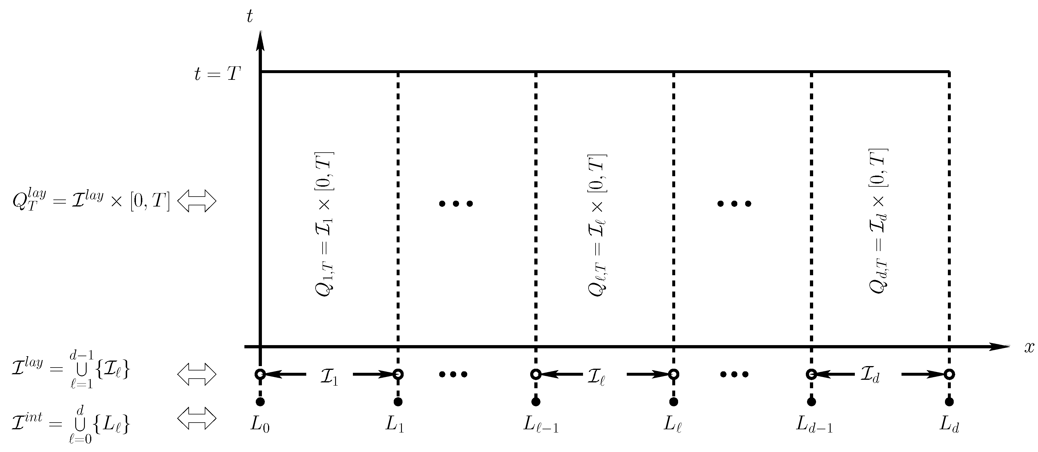
In this paper, we are interested in the problem of heat transfer in a multi-layered solid at very low temperatures. In order to make the mathematical model precise, let us consider a multi-layered solid of total length L, which is a compound of d-layers of lengths (see Figure 1) and introduce the notation (see Figure 2)
We suppose that the heat conduction on each layer is modeled on by a dual-phase-lagging equation, i.e.,
where and are the physical parameters and the heat source function on the ℓ-th layer, i.e., is the heat capacitance; and stand for the heat flux and the temperature gradient phase lags, respectively; is the conductivity; and is the heat source function. By notational convenience, we consider the piecewise constant functions and , the continuous function of the form
with the indicator function defined as if and otherwise. For each , the constant is the heat capacitance; and stand for the heat flux and the temperature gradient phase lags, respectively; is the conductivity; and is the heat source function. Hence, the mathematical model is given by the initial interface-boundary value problem
where and are some coefficients; and are the Knudsen numbers; and are the initial conditions; and are two given functions modelling the boundary conditions; and the bracket is defined by Here, with being a characteristic length and the boundary conditions (8) and (9) being models of the temperature-jump condition [14,20]. We recall that the Knudsen numbers are dimensionless quantities characterizing the boundary conditions of a flow defined as a ratio of the mean free path (the average distance traveled by each molecule between successive collisions) and the characteristic length of the flow (e.g., the diameter of a thruster) [21]. It is known that usually the Knudsen number cannot be measured by developing direct laboratory experiments and is defined by a non-linear regression. In that sense, the numerical values used in simulations are referred to as pseudo-Knudsen numbers. Moreover, following [14,20],we have that the relation of a Knudsen number and the heat conductivity k is given by where is a characteristic length and the parameter associated with is proportionally constant such that ,where is the wall-jumped temperature and is the unit outward normal vector on the boundary.
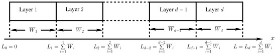
Figure 1.
Schematic representation of the multi-layered solid. For complete details of the notation, we refer to (4), where is defined to identify the position of the interfaces.
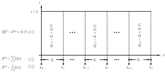
Figure 2.
Graphic representation of the notation defined in (4) and representing the physical domain.
We can reformulate the system (6)–(11) by introducing a change in variable. Let us consider the function such that , then the model (6)–(11), is rewritten as follows
where and .
By applying the finite difference method, we approximate the system (6)–(11). We follow the numerical approximations given in [14,22], where the authors consider a change in variable, a semi-discrete finite difference scheme for the new variable, a fully finite difference scheme for the new variable, and then approximate the original variable. The numerical scheme is developed by approximating (12)–(18) by a semidiscrete scheme and a fully discrete scheme. The methodology for the discretization of (12)–(18) consists of four steps: we approximate Equation (12) on the interior of each layer, we discretize appropriately interfaces (17) and (18), we approximate the boundary conditions (16), and we discretize Equation (13). Then, we deduce the finite difference numerical scheme approximating models (6)–(11) by using a the discrete version of the change variable. Roughly speaking, the numerical scheme for (6)–(11) consists of the solution of two linear systems of algebraic equations. Consequently, it is easy to implement.
The main results of the paper are the following: (i) we introduce semi-discrete and fully finite difference schemes to approximate the solution of (12)–(18); (ii) we introduce a full discrete finite difference scheme to approximate the solution of (6)–(11) and prove that this scheme is equivalent to the fully finite difference schemes for approximating (12)–(18); (iii) in the case of , we prove an energy estimate for u and v, satisfying the system (12)–(18) and also prove discrete energy estimate; (iv) we prove that the finite difference is unconditionally stable; (v) we prove an error estimate; and we introduce some numerical examples.
This paper is organized as follows. In Section 2, we introduce the finite difference schemes approximating (12)–(18) and (6)–(11). In Section 3, we introduce the analytical and numerical results. Finally, in Section 4 and Section 5, we present the numerical examples and the conclusiones of the work.
2. Finite Difference Approximation
2.1. Discretization of the Domain
Let us consider the notation in (4). We assume that each interval is divided into parts and that the temporal interval is divided into N parts. More precisely, to discretize the space and time domains, we select and consider that the ℓ-th layer and the time interval are divided into and N parts of sizes and respectively. To be precise in our analysis, we define the following notation and terminology:
It is important to note that is the discretization of the computational domain .
We describe the typical finite difference grid, norms and difference operators notation. We begin by defining the grid function space by
Let , then we introduce the finite difference operators and the finite difference notation
Moreover, for , we define the following notation:
for the inner product and norms on .
On the other hand, in the case of semidiscrete and discrete schemes, we use the notation
for respectively.
The finite difference discretization and error estimates will be developed by applying the following three Lemmas:
Lemma 1
([14,23]). Let us consider that is an interval partitioned in m sub-intervals of the form , where is defined by for with . If we consider that the function g is such that , then it holds that
Lemma 2
([23,24]). Consider that the function g is such that , then it holds that
Lemma 3
([14,23]). Consider that , then for any , it holds that
In a broad sense, Lemma 1 is applied to approximate the spatial derivatives, where relations (25) and (27) are used to approximate the second-order spatial derivatives on the boundaries and interfaces of the multi-layered solid and (26) inside each layer; Lemma 2 is used to approximate the time derivatives; and Lemma 3 is useful in the error estimate result.
2.2. Semidiscrete Scheme Approximating the Rewritten System
We construct the semidiscrete finite difference scheme for systems (12)–(18) by considering four steps. In the three first steps, we approximate (12) at the inside of each layer, the interfaces, and the boundaries, respectively. Meanwhile, in the fourth step, we approximate (13).
Step 1.
Approximation of (12) on . Here, we construct the semidiscrete scheme at inner grid points, i.e., except on the interfaces and boundaries. The inner grid points at are for . We start the discretization by considering Equation (12) at the inner grid points , then we have that
To discretize the right-hand side of (28), we can apply approximation (26) in Lemma 1 and observe that
for and . Dropping the small value terms in (29), replacing the approximation in (28), and using the notation (24), we deduce that the semidiscrete approximation form of (12) at the inner grid points is given by
Step 2.
Approximation of (12) on . Let us consider the interface points . We observe that the interface between the ℓ-th and -th layers is located at or . Let us consider the notation and . Then, considering the model Equation (12) at the inner grid points , we deduce that
To discretize the right-hand side of (31), we can apply the approximations (25) and (27) in Lemma 1, respectively; we observe that
The continuous interface condition given in (18) implies the following relationship:
Thus, from (31), dropping the small value terms in (32) and (33), using (34), and the notation (24), we obtain the semidiscrete approximation of the model equation at the interface points
In practice, one can replace and with and for , respectively. Hence,
Step 3.
Approximation of (12) on . We observe that the boundaries of the physical domain are located at and . Then, considering the evaluation of Equation (12) at the boundary points and , we deduce that
respectively. To discretize the right-hand sides of (37) and (38), we can apply the approximations (25) and (27) in Lemma 1, then, one can deduce the following relations:
respectively.
On the other hand, from (15) and (16), we have that
Replacing (41) and (42) in (39) and (40), respectively, and dropping the small value terms and replacing the approximations results in (37) and (38), respectively, we obtain the semidiscrete approximation at the boundaries
Step 4.
2.3. Fully Discrete Finite Difference Scheme Approximating the Rewritten System
In order to obtain the full discrete finite difference scheme, we consider the semidiscrete approximation and the evaluating each of semidiscrete relation at and , applying the Taylor expansion, Lemma 2 and adding the results, for , and we obtain the scheme
with the initial condition
2.4. Finite Difference Scheme Approximating the Original System
The finite difference scheme to obtain the numerical solution of (6)–(11) is given separately for and . More precisely, we have that the approximation (6)–(11) of
for . Meanwhile,
for . Moreover,
is the initial condition. We observe that the derivation of the finite difference scheme to solve the initial-interface boundary problems (6)–(11) is given by using the discrete schemes (47)–(52), and especially, the discrete version of the change of variable given in (51). More precisely, we have that the schemes (47)–(52) and (53)–(62) are equivalent (see Theorem 2).
3. Analytical and Numerical Analysis
3.1. Continuos Energy Estimation
We remark that model (6) (or equivalently (12)) corresponds to an energy balance since it originated in the energy Equation (1). It is well known that the function is called the energy for the heat equation . Moreover, the energy analysis implies some inequalities called energy estimates, which imply the stability and uniqueness of solutions. The following theorem gives the corresponding generalization of the standard heat equation estimates to the dual-phase-lagging multi-layered model.
Theorem 1.
3.2. Equivalence of Finite Difference Schemes for Rewritten and Original Systems
3.3. Discrete Energy Estimation
Theorem 3.
Proof.
Proof.
The proof is a consequence of Theorem 3. □
Theorem 5.
Proof.
From the definition, and satisfy the following relations:
with the initial condition for , and , the residuals of the Taylor series expansions, such that there exists a positive constant satisfying
for . We notice that the application of Lemma 2 implies that
which implies the estimates (83) and (84).
Let us consider the notation and . From (47)–(52) and (76)–(80), we have that satisfy the following scheme
for
We observe that the finite difference scheme (47)–(52) is similar to finite difference scheme (85)–(88) if we change by . Then, can develop the desired estimate by following similar algebraic procedures to the ones used in Theorem 3: multiplying (85)–(88) by , for , and respectively; summing up the results and using the following relations
and by making some rearrangements, we obtain the estimate
where
From (90) and (81)–(84), we deduce that there is a positive constant C such that . Then, replacing in (90), we deduce the estimate
which is equivalent to
Hence, we get (75) by observing that
by using the assumption , applying the Gronwall inequality, and Lemma 3. □
4. Numerical Examples
In this section, we present two numerical examples to test our finite difference scheme presented in Section 2. More precisely, the first example is a theoretical comparison between the numerical solution and the analytical solution. In addition, we give a test of error to verify the accuracy of Theorem 5.
The second example provides an application of the numerical scheme to nanoscale thin films of gold and chromium. In this case, we use the physical properties of these materials.
4.1. Example 1
In this example, we have followed the ideas of [22,25,26]. The chosen parameters are given in Table 1. It is important to note that some of the chosen parameters may not make physical sense because the main goal of this example is to compare the exact solution with the numerical solution to verify the accuracy of the our numerical scheme. We chose , and source terms

Table 1.
Parameters for Examples 1 and 2. is expressed in nm; in J/(m3 K); and in ps; and in W/(m K), where J: = joules; K: = kelvins; kg: = kilograms; m: = meters; nm: = nanometers; ps: = picoseconds; and W: = watts.
The initial conditions are
and
It is easy to see that the aforementioned problem has the following exact solution
In our simulations, we have considered , , . Also, the discretization parameters that have been used are , for ; and .
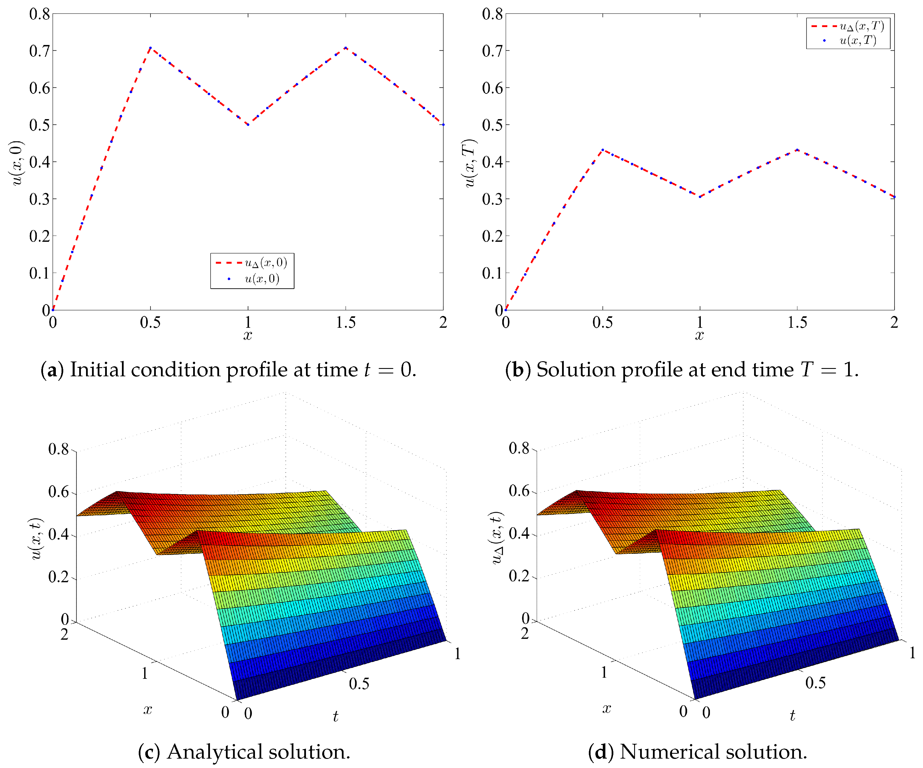
The comparison of the analytical solution and the numerical solution is given in Figure 3. On the one hand, in Figure 3a, we show the comparison of the initial condition between the exact solution and the numerical solution . Meanwhile, in Figure 3b, we show the comparison of the solution at final time between the exact solution and the numerical solution . On the other hand, in Figure 3c,d, we show the temperature distribution for every time for the exact solution and the numerical solution, respectively.

Figure 3.
Numerical results for Example 1. Here, and are the analytical solution and the numerical solution, respectively.
Now, consider the notation of Theorem 5. Then, from (22), one can define the -norm error between the analitycal solution and numerical solution as
For simplicity, we took . To calculate spatial convergence order, we use
for some fixed, sufficiently small . On the other hand, to calculate the temporal convergence order, we use
for some fixed, sufficiently small .
In the simulation test of spatial error, we chose the same quantity of grid points for each layer, that is, . Then, we test for and 80. The final time is , temporal discretization steps and time step . Results are shown in Table 2.
Table 2.
The spatial errors and convergence orders in -norm with .
On the other hand, for temporal errors, we fixed , and . We use different values for N and . Results are shown in Table 3.
Table 3.
The temporal errors and convergence orders in -norm with .
We conclude that the spatial convergence order is approximately 2. Meanwhile, the temporal order convergence is approximately 1. Results are consistent with the theoretical analysis from Theorems 4 and 5.
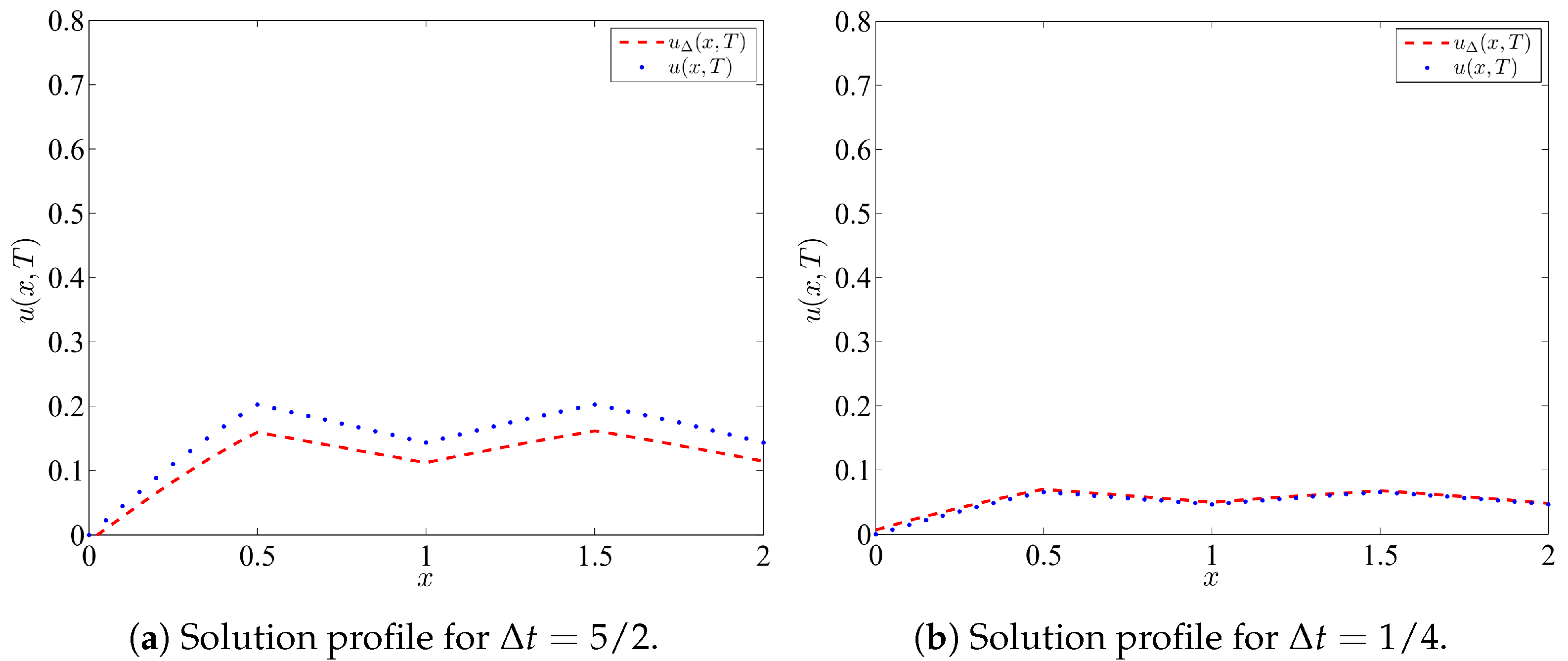
In addition, we verify that the precision of condition arises from Theorem 5 in a final long time . For this purpose, we consider , for , which implies . Then, for , we have and (see Figure 4a). On the other hand, if we consider , then and (see Figure 4b). Therefore, we conclude that if condition is not considered as time t increases, then the error between the analytical solution and the numerical solution also increases.
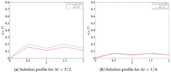
Figure 4.
Comparison between the analytical solution and the numerical solution for two different values of .
4.2. Example 2
We have based this example on the ideas of [11,14,27]. To be more precise, in the paper of [14], the authors consider a gold layer that is on a chromium padding layer and is irradiated by an ultrashort-pulsed laser. In our case, we consider four layers; the first and third layers are gold films of a size of nm. Meanwhile, the second and fourth layers are chromium films of a size of nm. This implies that the spatial domain is .
In Table 1 are specified properties of gold and chromium. The values of and have been obtained experimentally, while and are intrinsic properties of the materials provides in the literature [11]. Furthermore, following the ideas of [14,27], we can consider a laser heat source term widely used in dual-phase-lag (DPL) or two-temperature models as follows:
where F is fluence, R is surface reflectivity, is optical penetration depth, and is pulse duration. Then, if we take into account (2) and (6), then the source term can be considered as follows:
In this example, we took j/m2, nm, ps and . Therefore, the laser heat source term is
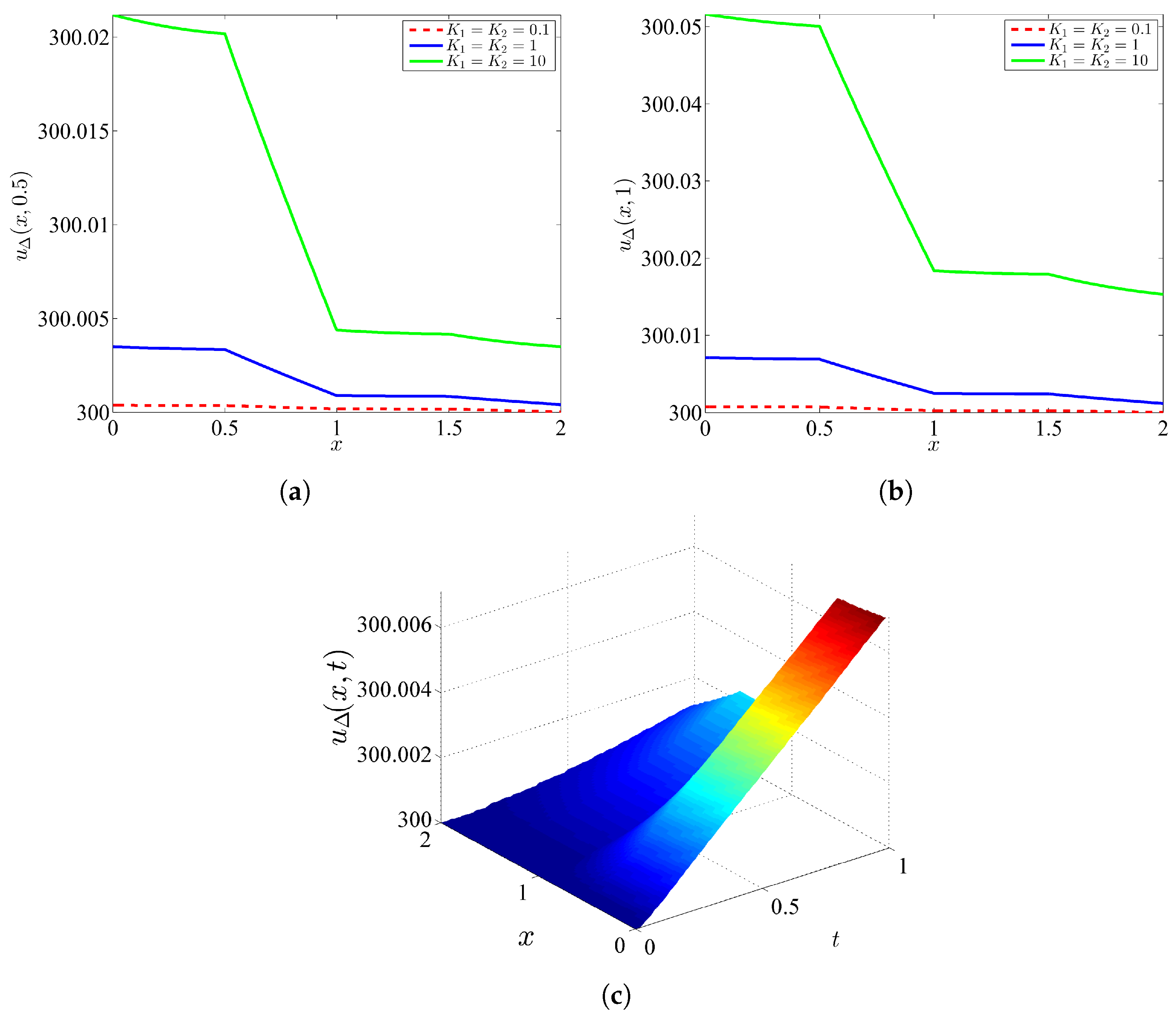
Furthermore, initial and boundary conditions are given by , and , respectively. These values are expressed in kelvins (K). In a physical sense, this means that the gold- and chromium-layer films are at room temperature. Additionally, there is no external flux, that is, . For the numerical simulation, we consider the spatial mesh partition , for , , and . We simulate for three Knudsen numbers and 10 in final times and 1. The results are shown in Figure 5. We specify that the Knudsen numbers used in this example are not real; however, they are commonly used in the literature (for more details, consult [21]).

Figure 5.
Numerical results for Example 2. (a,b) shown the numerical solution profile in kelvins at final time ps and ps, respectively, for different values of Knudsen numbers and 10. Figure (c) shows the numerical solution profile in domain and .
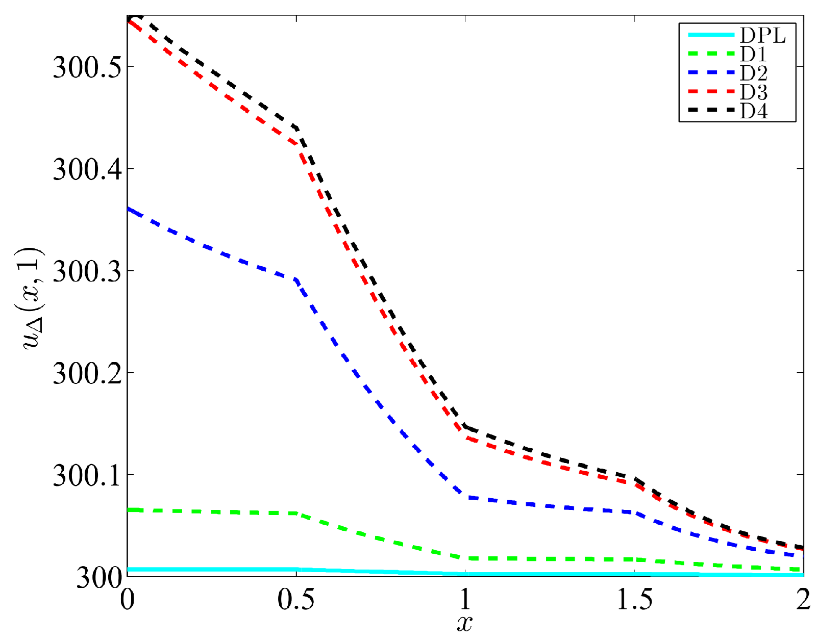
On the other hand, we consider the same initial and boundary conditions, , and provided in Table 1, and a fixed final time . In Figure 6, we illustrate the effects that occur when there is a decrease in phase lag, that is, when . The values used for and are shown in the Table 4.
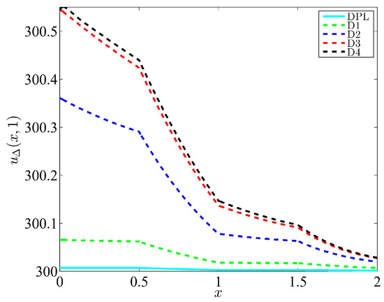
Figure 6.
Comparison of numerical solution for different values of and . The numerical values for each profile are given in Table 4.
Table 4.
Values of and for comparison of a decrease in phase lag.
We conclude that as the values of and decrease, the temperature begins to increase and starts to deviate from the phase-lag solution (DPL).
5. Conclusions and Future Work
We have introduced a mathematical model for the heat transfer phenomenon in multi-layered solids by considering a non-Fourier law. For modeling the interphases, we have assumed that the temperature and the heat flux are continuous. We have approximated the solution by introducing a finite difference scheme. We have proved some theoretical and numerical results; mainly, we have proved a continuous energy estimate, a discrete energy estimate, the unconditional stability of the numerical scheme, and an error estimate of the finite difference scheme. Moreover, we have validated our numerical approximation using analytical data and an example with parameter values close to industrial multi-layered solids composed of gold and chromium.
The results of this paper are deduced by assuming smooth conditions (on the coefficients and solution) and the energy estimates are deduced for the specific case of zero-flux boundary conditions. Hence, it will be interesting to study some extensions in a setting of more weak conditions and with other types of interface-boundary conditions. More precisely, we set out at least three issues that need more detailed exploration: (i) the study of the multi-layered dual-phase-lag equation with discontinuous interface conditions; (ii) the energy estimates in the case of non zero-flux boundary conditions or other kinds of boundary conditions; and (iii) the extension to multidimensional domains (see for instance [28]).
Author Contributions
Conceptualization A.C. and F.H.; methodology, A.C.; software, I.H.; validation, J.C.; formal analysis, A.C., F.H. and I.H.; investigation, A.C.; resources, A.C. and I.H.; data curation, J.C.; writing—original draft preparation, A.C.; writing—review and editing, A.C. and I.H.; visualization, F.H.; supervision, A.C. and I.H.; project administration, A.C. and I.H.; funding acquisition, A.C. and I.H. All authors have read and agreed to the published version of the manuscript.
Funding
This research was partially funded by Universidad Católica de Temuco; Universidad del Bío-Bío (Chile); the National Agency for Research and Development, ANID-Chile, through FONDECYT project 1230560; and by the Competition for Research Regular Projects, in the year of 2023, code LPR23-03, Universidad Tecnológica Metropolitana.
Data Availability Statement
The original files used to produce the simulations in the present work are available from the corresponding author upon reasonable request.
Conflicts of Interest
The authors declare no conflicts of interest.
References
- Dorfman, A.; Renner, Z. Conjugate Problems in Convective Heat Transfer: Review. Math. Probl. Eng. 2009, 2009, 927350. [Google Scholar] [CrossRef]
- Zudin, Y.B. Theory of Periodic Conjugate Heat Transfer, 3rd ed.; Springer: Berlin/Heidelberg, Germany, 2011. [Google Scholar]
- Kazemi-Kamyab, V.; van Zuijlen, A.H.; Bijl, H. A high order time-accurate loosely-coupled solution algorithm for unsteady conjugate heat transfer problems. Comput. Methods Appl. Mech. Eng. 2013, 264, 205–217. [Google Scholar] [CrossRef]
- Ooi, E.H.; van Popov, V. An efficient hybrid BEM–RBIE method for solving conjugate heat transfer problems. Comput. Math. Appl. 2014, 66, 2489–2503. [Google Scholar]
- Costa, R.; Nóbrega, J.M.; Clain, S.; Machado, G.J. Very high-order accurate polygonal mesh finite volume scheme for conjugate heat transfer problems with curved interfaces and imperfect contacts. Comput. Methods Appl. Mech. Eng. 2019, 357, 112560. [Google Scholar] [CrossRef]
- Pan, X.; Lee, C.; Choi, J.-I. Efficient monolithic projection method for time-dependent conjugate heat transfer problems. J. Comput. Phys. 2018, 369, 191–208. [Google Scholar] [CrossRef]
- Guo, S.; Feng, Y.; Tao, W.-Q. Deviation analysis of loosely coupled quasi-static method for fluid-thermal interaction in hypersonic flows. Comput. Fluids 2017, 149, 194–204. [Google Scholar] [CrossRef]
- Errera, M.-P.; Duchaine, F. Comparative study of coupling coefficients in Dirichlet-Robin procedure for fluid-structure aerothermal simulations. J. Comput. Phys. 2016, 312, 218–234. [Google Scholar] [CrossRef]
- Kazemi-Kamyab, V.; van Zuijlen, A.H.; Bijl, H. Analysis and application of high order implicit Runge-Kutta schemes for unsteady conjugate heat transfer: A strongly-coupled approach. J. Comput. Phys. 2014, 272, 471–486. [Google Scholar] [CrossRef]
- Dai, W.; Han, F.; Sun, Z. Accurate numerical method for solving dual-phase-lagging equation with temperature jump boundary condition in nano heat conduction. Int. J. Heat Mass Transf. 2013, 64, 966–975. [Google Scholar] [CrossRef]
- Tzou, D.Y. A unified field approach for heat conduction from macro-to micro-scale. ASME J. Heat Transf. 1995, 117, 8–16. [Google Scholar] [CrossRef]
- Tzou, D.Y. Macro to Microscale Heat Transfer. The Lagging Behaviour, 2nd ed.; Taylor & Francis: Washington, DC, USA, 2014. [Google Scholar]
- Borjalilou, V.; Asghari, M. Small-scale analysis of plates with thermoelastic damping based on the modified couple stress theory and the dual-phase-lag heat conduction model. Acta Mech. 2018, 229, 124720. [Google Scholar] [CrossRef]
- Sun, H.; Sun, Z.Z.; Dai, W. A second-order finite difference scheme for solving the dual-phase-lagging equation in a double-layered nano-scale thin film. Numer. Methods Partial. Differ. Equ. 2017, 33, 142–173. [Google Scholar] [CrossRef]
- Cattaneo, C. A Form of Heat Conduction Equation Which Eliminates the Paradox of Instantaneous Propagation. C. R. Acad. Sci. 1958, 247, 431–433. [Google Scholar]
- Quintanilla, R. Exponential stability in the dual-phase-lag heat conduction theory. Int. J. Heat Mass Transf. 2002, 27, 217–227. [Google Scholar] [CrossRef]
- Quintanilla, R.; Racke, R. A note on stability in dual-phase-lag heat conduction. Int. J. Heat Mass Transf. 2006, 49, 1209–1213. [Google Scholar] [CrossRef]
- Kumar, S.; Srivastava, A. Thermal analysis of laser-irradiated tissue phantoms using dual phase lag model coupled with transient radiative transfer equation. Int. J. Heat Mass Transf. 2015, 90, 466–479. [Google Scholar] [CrossRef]
- Poshti, A.G.T.; Khosravirad, A.; Ayani, M.B. Analyses of non-Fourier heat conduction in 1-D spherical biological tissue based on dual-phase-lag bio-heat model using the conservation element/solution element (CE/SE) method: A numerical study. Int. Commun. Heat Mass Transf. 2022, 132, 105881. [Google Scholar] [CrossRef]
- Ghazanfarian, J.; Abbassi, A. Effect of boundary phonon scattering on Dual-Phase-Lag model to simulate micro- and nano-scale heat conduction. Int. J. Heat Mass Transf. 2009, 52, 3706–3711. [Google Scholar] [CrossRef]
- Rapp, B. Microfluidics: Modeling, Mechanics and Mathematics; Elsevier: Amsterdam, The Netherlands, 2016. [Google Scholar]
- Coronel, A.; Huancas, F.; Lozada, E.; Tello, A. A Numerical Method for a Heat Conduction Model in a Double-Pane Window. Axioms 2022, 11, 422. [Google Scholar] [CrossRef]
- Sun, Z.Z. Numerical Methods for Partial Differential Equations, 2nd ed.; Science Press: Beijing, China, 2012. [Google Scholar]
- Liao, H.L.; Sun, Z.Z. Maximum norm error estimates of efficient difference schemes for second-order wave equations. J. Comput. Appl. Math. 2011, 235, 2217–2233. [Google Scholar] [CrossRef]
- Coronel, A.; Lozada, E.; Berres, S.; Fernando, F.; Murúa, N. Mathematical modeling and numerical approximation of heat conduction in three-phase-lag solid. Energies 2024, 17, 2497. [Google Scholar] [CrossRef]
- Murúa, N.; Coronel, A.; Tello, A.; Berres, S.; Huancas, F. GPU Accelerating Algorithms for Three-Layered Heat Conduction Simulations. Mathematics 2024, 12, 3503. [Google Scholar] [CrossRef]
- Zhang, Y.; Tzou, D.Y.; Chen, J.K. Micro- and nanoscale heat transfer in femtosecond laser processing of metals. In High-Power and Femtosecond Lasers: Properties, Materials and Applications; Nova Science Publishers: Hauppauge, NY, USA, 2009; pp. 159–206. [Google Scholar]
- Liu, C.; Cao, W.; Song, X.; Wan, Y. A semi-analytical method of three-dimensional dual-phase-lagging heat conduction model. J. Heat Mass Transf. 2024, 218, 124720. [Google Scholar] [CrossRef]

Disclaimer/Publisher’s Note: The statements, opinions and data contained in all publications are solely those of the individual author(s) and contributor(s) and not of MDPI and/or the editor(s). MDPI and/or the editor(s) disclaim responsibility for any injury to people or property resulting from any ideas, methods, instructions or products referred to in the content. |
© 2025 by the authors. Licensee MDPI, Basel, Switzerland. This article is an open access article distributed under the terms and conditions of the Creative Commons Attribution (CC BY) license (https://creativecommons.org/licenses/by/4.0/).