Inertial Algorithm for Best Proximity Point, Split Variational Inclusion and Equilibrium Problems with Application to Image Restorations

Abstract

If S and T are two non-self-mappings, then a solution of equation $S{a}^{*}=T{a}^{*}=a^{*}$ does not necessarily exist. The common best proximity point problem is to find the approximate optimal solution of such type of equation and have a key role in theory of approximation and optimization. The primary goal of this paper is to introduce an inertial-type self-adaptive algorithm for solving the common best proximity point, generalized equilibrium and split variational inclusion problems in Hilbert spaces. The strong convergence of the proposed algorithm is given under some mild conditions. It is worth mentioning that the step size in many existing algorithms requires the prior knowledge of operator norms which is difficult to compute, whereas our proposed algorithm does not require this condition. Numerical examples are given to illustrate the efficiency and applicability of the proposed approach. We further apply the proposed algorithm to an image restoration problem and show that it achieves a higher signal-to-noise ratio compared with the existing algorithms considered in this study.

1. Introduction and Preliminaries

Optimization, variational inclusion, equilibrium and best proximity point problems are well-known classes of nonlinear problems with numerous applications in applied sciences and engineering. The search for efficient, low cost, flexible and easily implementable iterative algorithms to approximate common solutions of such problems has been an active area of research over the last few decades. In this continuation, we propose an efficient algorithm to approximate the common solution of these problems.

Throughout this paper, $\mathbb{R}$ and $\mathbb{N}$ denote the sets of all real and natural numbers, respectively. The notations $a_n\to a^{*}$ and $a_n\rightharpoonup a^{*}$ represent strong and weak convergence, respectively, while $\chi \left(a_n\right)$ denotes the set of weak limit points of the sequence $\left\{a_n\right\}$.

Suppose that $\mathcal{H}$ is a real Hilbert space and C is a nonempty closed convex subset of $\mathcal{H}$. A mapping $T:C\to C$ is said to be nonexpansive if $\parallel Ta-Tb\parallel \le \parallel a-b\parallel ,\forall a,b\in C$. Such mappings arise frequently in convex optimization, economics, signal processing, image reconstruction, variational inclusion and other applied sciences (see, e.g., [1,2]).

Let C and D be nonempty subsets of $\mathcal{H}$ with $C^{*}\subset C$. A mapping $T:C^{*}\to D$ is called $C^{*}$-nonexpansive if $\parallel Ta-Tc\parallel \le \parallel a-c\parallel ,\forall a\in C,c\in C^{*}.$

Let us recall some other concepts needed in the sequel. A multi-valued mapping T is monotone, if for $a^{\prime }\in Ta$ and $b^{\prime }\in Tb,$ we have the following: $\langle a-b,a^{\prime }-b^{\prime }\rangle \ge 0,$ where $a,b\in \mathcal{H}$. Note that if the graph of T is not properly contained in the graph of another monotone mapping then the mapping T is known as maximal monotone. For $\lambda >0$ and I, the identity operator, the resolvent operator T is given as follows:

$$J_{\lambda }^T={(I+\lambda T)}^{-1};$$

A self-mapping T on $\mathcal{H}$ is said to k-inversely monotone if, for all $a,b\in \mathcal{H}$,

$$\langle a-b,Ta-Tb\rangle \ge {k\parallel Ta-Tb\parallel }^2,$$

where $k>0$ is a constant. In particular, when $k=1$, the operator T is referred to as inverse strongly monotone (firmly nonexpansive).

Note that for any $h_1\in \mathcal{H}$, there is an element $P_C{h}_1\in C$ such that

$$\parallel h_1-P_C{h}_1\parallel =inf\{\parallel h_1-h_2\parallel :h_2\in C\}.$$

The mapping $P_C:\mathcal{H}\to C$ is known as metric projection, and the element $P_C{h}_1$ is referred to as the best approximation of $h_1$ from C.

Note that for any $h_1\in \mathcal{H}$,

$$P_C{h}_1=h_3\mathrm{if}\mathrm{and}\mathrm{only}\mathrm{if}\langle h_1-h_3,h_3-h_2\rangle \ge 0,\mathrm{for}\mathrm{all}{h}_2\in C.$$

(1)

For more details on metric projections, we refer to Section 3 of [3,4].

The projection mapping $P_C$ is a classical example of firmly nonexpansive mappings; consequently, it is also nonexpansive (see Section 11 in [3]). Moreover, a mapping $T:C\to \mathcal{H}$ is said to be demiclosed on C if the operator $I-T$ has a graph that is sequentially closed with respect to weak convergence in the domain and strong convergence in the codomain.

Lemma 1

([5]). Assume that $T:C\to \mathcal{H}$ is a nonexpansive mapping, then we have $I-T$ demiclosed at zero, i.e., for any sequence $\left\{h_n\right\}\subset C$ such that $h_n\rightharpoonup h_1$ and $(I-T)h_n\to 0$, it follows that $(I-T)h_1=0$.

Definition 1

([6]). A function $T:\mathcal{H}\to \mathbb{R}\cup \{+\infty \}$ is said to be weakly lower semi-continuous at a point $h^{*}\in \mathcal{H}$ if, for any sequence $\left\{h_n\right\}$ in $\mathcal{H}$ with $h_n\rightharpoonup h^{*}$, we have

$$T\left(h^{*}\right)\le \underset{n\to \infty }{lim\; inf}T\left(h_n\right).$$

Lemma 2

([7]). For any $h_1,h_2\in \mathcal{H}$ and $\delta \in \mathbb{R}$, the following equalities and inequalities hold:

(i)   

${\parallel h_1+h_2\parallel }^2\le 2\langle h_1+h_2,h_2\rangle +{\parallel h_1\parallel }^2$,

(ii)  

${\parallel h_1+h_2\parallel }^2={\parallel h_1\parallel }^2+{\parallel h_2\parallel }^2+2\langle h_1,h_2\rangle$,

(iii) 

${\parallel h_1-h_2\parallel }^2={\parallel h_1\parallel }^2+{\parallel h_2\parallel }^2-2\langle h_1,h_2\rangle$,

(iv) 

${\parallel \delta h_1+(1-\delta )h_2\parallel }^2=\delta {\parallel h_1\parallel }^2+(1-\delta ){\parallel h_2\parallel }^2-\delta (1-\delta ){\parallel h_1-h_2\parallel }^2$.

Lemma 3

([8]). For any $h_1,h_2,h_3\in \mathcal{H}$ and $\rho ,\eta ,\theta \in [0,1]$ with $\rho +\eta +\theta =1$, the following identity holds:

$${\parallel \rho h_1+\eta h_2+\theta h_3\parallel }^2=\rho {\parallel h_1\parallel }^2+\eta {\parallel h_2\parallel }^2+\theta {\parallel h_3\parallel }^2-\rho \eta {\parallel h_1-h_2\parallel }^2-\eta \theta {\parallel h_2-h_3\parallel }^2-\rho \theta {\parallel h_1-h_3\parallel }^2.$$

Lemma 4

([9]). Let $\left\{{\overline{a}}_n\right\},\left\{{\overline{c}}_n\right\}\subset {\mathbb{R}}^{+}$ and $\left\{{\overline{b}}_n\right\}\subset \mathbb{R}$, $\left\{{\delta }_n\right\}\subset (0,1)$ such that ${\sum }_{n=0}^{\infty }{\overline{c}}_n<\infty$. Suppose

$${\overline{a}}_{n+1}\le (1-{\delta }_n){\overline{a}}_n+{\overline{b}}_n+{\overline{c}}_n,\forall n\ge 0.$$

       The following conclusions hold:

(i)  

If there exists a constant $\theta \ge 0$ such that ${\overline{b}}_n\le \theta {\delta }_n$, then the sequence $\left\{{\overline{a}}_n\right\}$ is bounded.

(ii) 

If ${\sum }_{n=0}^{\infty }{\delta }_n=\infty$ and $\underset{n\to \infty }{lim\; sup}{\displaystyle \frac{{\overline{b}}_n}{{\delta }_n}}\le 0$, then ${\overline{a}}_n\to 0$ as $n\to \infty$.

Lemma 5

([10]). Let $\left\{{\overline{a}}_n\right\}\subset {\mathbb{R}}^{+}$ and $\left\{{\delta }_n\right\}\subset (0,1)$ satisfy ${\sum }_{n=0}^{\infty }{\delta }_n=\infty$. Let $\left\{{\overline{b}}_n\right\}\subset \mathbb{R}$ and assume that

$${\overline{a}}_{n+1}\le (1-{\delta }_n){\overline{a}}_n+{\delta }_n{\overline{b}}_n,\forall n\in \mathbb{N}.$$

If $\underset{n\to \infty }{lim\; sup}{\overline{b}}_{n_i}\le 0$ and for any subsequence $\left\{{\overline{a}}_{n_i}\right\}$ of $\left\{{\overline{a}}_n\right\}$ satisfying $\underset{i\to \infty }{lim\; inf}({\overline{a}}_{n_{i+1}}-{\overline{a}}_{n_i})\ge 0$, then it follows that $\underset{n\to \infty }{lim}{\overline{a}}_n=0$.

Assume that ${\mathcal{H}}_1$ and ${\mathcal{H}}_2$ are real Hilbert spaces, and let C and D be nonempty closed convex subsets of ${\mathcal{H}}_1$ and ${\mathcal{H}}_2$, respectively. Suppose that $A:{\mathcal{H}}_1\to {\mathcal{H}}_2$ is a bounded linear operator.

Let $F:C\times C\to \mathbb{R}$ be a bifunction. The corresponding equilibrium problem (EP) is to obtain $a^{*}\in C$ such that

$$F(a^{*},b)\ge 0,\forall b\in C.$$

If $G:C\to \mathcal{H}$ is a given operator, then the variational inequality problem (VIP) is formulated as

$$\mathrm{Find}\mathrm{an}\mathrm{element}{a}^{*}\in C\mathrm{such}\mathrm{that}\langle b-a^{*},G{a}^{*}\rangle \ge 0,\forall b\in C.$$

By combining these two concepts, we obtain the generalized equilibrium problem associated with F and G, denoted by $GEP(F,G)$, which can be formulated as follows: for any $b\in C$, find $a^{*}\in C$; we have

$$F(a^{*},b)+\langle b-a^{*},G{a}^{*}\rangle \ge 0,$$

(2)

It is clear that if $G=0$ in (2), $GEP(F,G)$ simplifies to the standard EP. Likewise, if $F=0$ in (2), it reduces to the VIP. The set of all solutions of $GEP(F,G)$ is represented by $\mathcal{S}\left(GEP\right(F,G\left)\right)$.

It is worth mentioning that $GEP(F,G)$ provides a unified framework that includes several important mathematical models such as optimization problems, equilibrium, and Nash equilibrium variational inequalities problems. For more detailed discussions, one can see [11,12,13,14].

Assume $C_1,C_2\subset \mathcal{H}$ which are also closed and convex; $T:C_1\to C_2$ is a mapping. The distance between two sets is given as follows:

$$d(C_1,C_2)=inf\{\parallel c^{\prime }-c^{″}\parallel :c^{\prime }\in C_1\mathrm{and}{c}^{″}\in C_2\}.$$

The best proximity point problem (BPP) is formulated as follows: find $a^{*}\in C_1$ with

$$\parallel a^{*}-T{a}^{*}\parallel =d(C_1,C_2),$$

(3)

where $d(C_1,C_2)$ denotes the distance between sets $C_1$ and $C_2$.

The BPP has a key role in optimization (see [15,16,17]) and includes the fixed point as a special case. Several methods have been proposed in the literature to solve the BPP (see [18,19,20,21]). We denote the solution set of BPP by $\mathcal{B}\left(T\right)$ for a given mapping T. Moreover, if T is a $C^{*}$-nonexpansive mapping and we take $C^{*}=\mathcal{B}\left(T\right)$, in this case, T is referred to as a best proximally nonexpansive mapping.

The split inverse problem (SIP) is described as follows:

Find a point

$$a^{*}\in {\mathcal{H}}_1\mathrm{that}\mathrm{can}\mathrm{solve}I{P}_1$$

and

$$A{a}^{*}\in {\mathcal{H}}_2\mathrm{that}\mathrm{can}\mathrm{solve}I{P}_2,$$

where $I{P}_1$ and $I{P}_2$ are the inverse problems posed in the spaces ${\mathcal{H}}_1$ and ${\mathcal{H}}_2$, respectively, and $A:{\mathcal{H}}_1\to {\mathcal{H}}_2$ is an operator.

Similarly, SVIP (split variational inclusion problem) is formulated as follows:

Find an element

$$a^{*}\in {\mathcal{H}}_1\mathrm{which}\mathrm{satisfies}0\in L_1{a}^{*},$$

and

$$A{a}^{*}\in {\mathcal{H}}_2\mathrm{which}\mathrm{satisfies}0\in L_{2}A{a}^{*},$$

where $L_1$ and $L_2$ are multi-valued mappings on ${\mathcal{H}}_1$ and ${\mathcal{H}}_2$, respectively.

Many practical problems in applied sciences can be modeled using SVIP (see, for example, [22,23]). In the sequel, $\Gamma$ denotes the solution set of SVIP and $C_1$ and $C_2$ are closed and convex sets.

Remark 1

([24,25]). Note that we have the following facts:

• A mapping L is maximal monotone if and only if $J_{\lambda }^L$ is a single value.
• $J_{\lambda }^L{a}^{*}=a^{*}$ if and only if $a^{*}\in L^{-1}\left(0\right).$
• The SVIP is equivalent to the following:
  Find $a^{*}\in {\mathcal{H}}_1$ with

  $$J_{\lambda }^{L_1}{a}^{*}=a^{*}withA{a}^{*}\in {\mathcal{H}}_{2}andA{a}^{*}=J_{\lambda }^{L_2}A{a}^{*}.$$

  (4)

Let $C_1,C_2\subset {\mathcal{H}}_1$. Define $C_0$ and $D_0$ as follows:

$$C_0=\{a^{\prime }\in C_1: \parallel a^{\prime }-b^{\prime }\parallel =D(C_1,C_2),\mathrm{for}\mathrm{some}{b}^{\prime }\in C_2\}$$

and

$$D_0=\{b^{\prime }\in C_2: \parallel a^{\prime }-b^{\prime }\parallel =D(C_1,C_2),\mathrm{for}\mathrm{some}{a}^{\prime }\in C_1\}.$$

Lemma 6

([18]). Let $C_1,C_2\subset \mathcal{H}$, and let $T:C_1\to C_2$ be a mapping such that $T\left(C_0\right)\subseteq D_0$. Then, any fixed point of the composition $P_{C_1}T$ within $C_0$ gives the best proximity point of T.

Definition 2

([26]). If $C_1$ and $C_2$ are subset a metric space $(X,d)$. We say that $C_1$ and $C_2$ satisfy the P-property if, for any $a_1,a_2\in C_0$ and $b_1,b_2\in D_0$, the following condition holds:

$$d(a_1,b_1)=d(a_2,b_2)=D(C_1,C_2)\Rightarrow d(a_1,a_2)=d(b_1,b_2).$$

Lemma 7

([19]). If $C_1,C_2\subset \mathcal{H}$, and $T:C_1\to C_2$ satisfy $T\left(C_0\right)\subseteq D_0$, then ${T|}_{C_0}$ has the proximal property iff the operator $(I-P_{C_1}T){|}_{C_0}$ is demiclosed at zero.

To approximate the solutions of nonlinear problems, different iterative algorithms have been widely studied and proposed in the literature ([27,28,29,30,31]). For example, Abbas et al., [32] proposed an algorithm called an AA-iteration scheme, where the proposed sequence $\left\{a_n\right\}$ is given as Algorithm 1:

Algorithm 1: AA-iteration

Initialization: Assume $\left\{{\alpha }_n\right\}$, $\left\{{\beta }_n\right\},\left\{{\gamma }_n\right\}\subset (0,1)$. Set any $a_1\in C$; calculate $a_{n+1}$ in the following ways: $$\begin{array}{cc}& d_n=(1-{\gamma }_n)a_n+{\gamma }_{n}T{a}_n,\hfill \\ & c_n=T((1-{\beta }_n)d_n+{\beta }_{n}T{d}_n),\hfill \\ & b_n=T((1-{\alpha }_n)T{d}_n+{\alpha }_{n}T{c}_n),\hfill \\ & a_{n+1}=T{b}_n.\hfill \end{array}$$

The authors in [32] proved that the sequence generated by an AA-iteration scheme converges faster than many well-known comparable schemes. After that, several authors have applied the AA-algorithm to solve certain nonlinear problems; see [33,34,35,36].

Byrne et al. [37] proposed an iterative algorithm for SVIP involving $L_1$ and $L_2$ which are maximal monotone, and the proposed sequence is given as follows in Algorithm 2.

Algorithm 2: Byrne’s algorithm

Initialization: Suppose that $\left\{{\alpha }_n\right\}$ is a sequence in $(0,1)$, $\lambda \ge 0$ and $\sigma \in (0,{\displaystyle \frac{2}{K}}),$   where $K=\parallel A^{*}A\parallel$. For $a_1\in {\mathcal{H}}_1$, calculate $a_{n+1}$ as follows: $$a_{n+1}={\alpha }_n{a}_n+(1-{\alpha }_n)J_{\lambda }^{L_1}(a_n+\sigma A^{*}(J_{\lambda }^{L_2}-I)A{a}_n).$$

    Finding a common solution for various nonlinear problems has attracted significant attention in recent research. For example, Ref. [38] introduced an iterative sequence to compute a common solution of fixed point problems and SVIP for nonexpansive mappings. The proposed sequence is described as in Algorithm 3.

Algorithm 3: Wangkeeree’s algorithm

Initialization: Let $\left\{{\alpha }_n\right\}\subset (0,1)$, $\lambda \ge 0$ and $\sigma \in (0,{\displaystyle \frac{2}{K}})$, where K is as given above.   Choose any $a_1\in {\mathcal{H}}_1$, find $a_{n+1}$ as: $$b_n=J_{\lambda }^{L_1}(a_n+\sigma A^{*}(J_{\lambda }^{L_2}-I)A{a}_n)$$ $$a_{n+1}={\alpha }_n\eta \Phi a_n+(1-{\alpha }_{n}S)T{b}_n.$$

In the algortithm, $\Phi$ and T are the contraction and nonexpansive mappings on ${\mathcal{H}}_1$, respectively, and S is operator that is bounded linear on ${\mathcal{H}}_1$. Authors have shown that the sequence defined in Algorithm 3 converges the unified solution of the problems mentioned above.

In 2021, Suntai [39] introduced an iterative algorithm to address the BPP and EP. The algorithm is formulated as Algorithm 4.

Recently, Husain et al. [40] proposed an iterative sequence for solution of BPP and generalized GEP. The proposed algorithm is given in Algorithm 5.

Algorithm 4: Suntai’s algorithm

Initialization: Let $\left\{{\alpha }_n\right\}\subset (0,1)$ with ${lim\; sup}_{n\to \infty }{\alpha }_n<1$ and $\tau \in \left(0,{\displaystyle \frac{1}{\parallel A^{*}{\parallel }^2}}\right)$. Set   any $a_0\in C_0$, find $a_{n+1}$ as follows: $$\begin{array}{cc}& c_n=(1-{\alpha }_n)a_n+{\alpha }_n{P}_{C}T{a}_n,\hfill \\ & b_n=P_C\left[c_n+\tau A^{*}(G_{r_n}^F-I)A{c}_n\right],\hfill \\ & C_{n+1}=\{d\in C_n:\parallel b_n-d\parallel \le \parallel c_n-d\parallel \le \parallel a_n-d\parallel \},\hfill \\ & a_{n+1}=P_{C_{n+1}}\left(a_0\right).\hfill \end{array}$$

Algorithm 5: Husain’s algorithm

Initialization: Let $\left\{{\alpha }_n\right\},\left\{{\delta }_n\right\}\subset (0,1)$, $\tau \in \left(0,{\displaystyle \frac{1}{\parallel A^{*}{\parallel }^2}}\right)$. Set any $a_0,a_1\in C_0$,   calculate $a_{n+1}$ as follows: $$\begin{array}{cc}& c_n=a_n+{\delta }_n(a_n-a_{n-1}),\hfill \\ & b_n=(1-{\alpha }_n)c_n+{\alpha }_n{P}_{C_1}T{c}_n,\hfill \\ & a_{n+1}=P_{C_1}(b_n+\tau A^{*}(V-I)A{b}_n),\hfill \end{array}$$

    In the algorithm, $V=G_{r_n}^F(I-r_{n}G)$, $r_n\subset (0,\infty )$.

The choice of step size is crucial in any iterative method, as it directly influences both the computational process and the convergence speed. The selection of an appropriate step size can lead to faster approximation of the solution, thereby improving the overall rate of convergence of the iterative scheme. Furthermore, incorporating an inertial term based on the previous two iterations can help accelerate the convergence of iterative algorithms. Various researchers have developed and applied algorithms that combine inertial terms with self-adaptive step sizes to approximate solutions of nonlinear operator equations (see, for example, [40,41]). This naturally raises a question: Can we design an iterative algorithm that achieves faster convergence to the common solution of some general nonlinear problems?

Motivated by the aforementioned studies, this paper introduces an efficient inertial-type algorithm for approximating the common solution of several nonlinear problems. Obtaining the unified solution instead of addressing each problem individually provides a unified perspective on the interrelated variables. This strategy yields a more complete understanding of the system’s behavior and ensures consistency complex cases.

Remark 2.

Unlike the shrinking projection and explicit schemes in the literature (e.g., [39,40,42]), our proposed algorithm uses a self-adaptive step size that does not require prior knowledge of the operator norm, which is a structural difference in the step size. Further, we relax several restrictive assumptions commonly used in existing work, for example, explicit norm-bounds or shrinking parameters. To the best of our knowledge, in the existing literature, the inertial projection algorithms are used to solve the split best proximity or at most a combination of best proximity and equilibrium problems.Our scheme is formulated as an inertial type self-adaptive iteration that can approximate the solution of the common best proximity, generalized equilibrium and split variational inclusion problems in one unified framework. We provide both theoretical and practical contribution and the applicability of inertial technique to a broader class of coupled problems. Numerical experiments and image restorations illustrate that the our proposed approach is superior and gives high signal-to-noise ratio in relation t comparable schemes.

2. Convergence Analysis

Assumption A1

([41]). Let $F:C\times C\to \mathbb{R}$ and $G:{\mathcal{H}}_1\to {\mathcal{H}}_1$. To solve the generalized equilibrium problem $GEP(F,G)$, we impose the following conditions on F and G:

$\left(A_1\right)$

$F(a,a)=0$,

$\left(A_2\right)$

$F(a,b)+F(b,a)+\langle Ga,b-a\rangle +\langle Gb,a-b\rangle \le 0$,

$\left(A_3\right)$

$F(b,c)\ge {lim}_{\alpha \downarrow 0}F(\alpha a+(1-\alpha )b,c)$,

$\left(A_4\right)$

the function $b\mapsto F(a,b)+\langle Ga,b-a\rangle$ is lower semi-continuous and convex, for all $a,b,c\in C$.

Definition 3

([41]). For a given $r>0$, define the operator $G_r^F:{\mathcal{H}}_1\to 2^C$ by

$$G_r^F\left(a^{\prime }\right)=\left\{c^{\prime }\in C:{\displaystyle \frac{1}{r}}\langle b^{\prime }-c^{\prime },c^{\prime }-a^{\prime }\rangle +F(c^{\prime },b^{\prime })+\langle G{c}^{\prime },b^{\prime }-c^{\prime }\rangle \ge 0,\forall b^{\prime }\in {\mathcal{H}}_1\right\}.$$

(5)

Lemma 8

([41]). If we use $\left(A_1\right)-\left(A_4\right)$, the operator $G_r^F$ satisfies the following properties:

(1) 

$G_r^F$ is single-valued and firmly nonexpansive.

(2) 

The fixed point of $G_r^F$ solve the $GEP(F,G)$.

(3) 

The fixed point set of the mapping $G_r^F$ is convex and closed.

Proposed Algorithm

Take $C_i,C\subset {\mathcal{H}}_1$ and $D_i,D\subset {\mathcal{H}}_2$ for $i=1,2$ which are also convex and closed. Assume that $F:C\times C\to \mathbb{R}$ satisfies Assumption A1, $A^{*}$ denotes the adjoint of a bounded linear operator A from ${\mathcal{H}}_1$ to ${\mathcal{H}}_2$. Consider $S,T:C_1\to C_2$ as best proximally nonexpansive mappings and $\Phi :{\mathcal{H}}_1\to {\mathcal{H}}_1$ as contraction with $\theta$ as contraction constant.

The following functions are defined as follows:

$$\begin{array}{cc}\hfill f_1\left(a\right)& ={\displaystyle \frac{1}{2}}\parallel (I-J_{{\lambda }_2}^{L_2})Aa{\parallel }^2,\hfill \\ \hfill f_2\left(a\right)& ={\displaystyle \frac{1}{2}}\parallel (I-J_{{\lambda }_1}^{L_1})a{\parallel }^2,\hfill \\ \hfill M\left(a\right)& =A^{*}(I-J_{{\lambda }_2}^{L_2})Aa,\hfill \\ \hfill N\left(a\right)& =(I-J_{{\lambda }_1}^{L_1})a.\hfill \end{array}$$

Here, $f_1$ and $f_2$ are differentiable, weakly lower semi-continuous, and convex [43], while M and N are Lipschitz continuous [25]. The proposed iterative algorithm is now described in Algorithm 6.

Algorithm 6: Proposed algorithm

Step 0. Initialize $a_0,a_1\in \mathcal{H}$ and a non-negative parameter $\delta$. Set $n=1$. Step 1. For the $(n-1)$th and nth iterates, select ${\delta }_n$ satisfying $0\le {\delta }_n\le {\widehat{\delta }}_n$, where $$\begin{array}{c}\hfill {\widehat{\delta }}_n=\left\{\begin{array}{cc}min\left\{\delta ,{\displaystyle \frac{{\tau }_n}{\parallel a_n-a_{n-1}\parallel }}\right\},\hfill & \mathrm{for}{a}_n\ne a_{n-1},\hfill \\ \delta ,\hfill & \mathrm{else}.\hfill \end{array}\right.\end{array}$$ (6) Step 2. Calculate $$e_n=a_n+{\delta }_n(a_n-a_{n-1}).$$ Step 3. Compute $d_n\in C_1$ which satisfies $${\displaystyle \frac{1}{r_n}}\langle a^{*}-d_n,d_n-e_n\rangle +F(d_n,a^{*})+\langle G{d}_n,a^{*}-d_n\rangle \ge 0,\forall a^{*}\in \mathcal{H}.$$ Step 4. Find $$c_n={\eta }_n{e}_n+(1-{\eta }_n)d_n.$$ Step 5. Find $$b_n=P_C\left(J_{{\lambda }_1}^{L_1}(I-{\sigma }_n{A}^{*}(I-J_{{\lambda }_2}^{L_2})A)c_n\right),$$ where $${\sigma }_n=\left\{\begin{array}{cc}{\displaystyle \frac{{\mu }_n{f}_1\left(c_n\right)}{\parallel M\left(c_n\right){\parallel }^2+{\parallel N\left(c_n\right)\parallel }^2}}\hfill & \mathrm{if}\parallel M\left(c_n\right){\parallel }^2+{\parallel N\left(c_n\right)\parallel }^2\ne 0\hfill \\ 0\hfill & \mathrm{otherwise}.\hfill \end{array}\right.$$ (7) Step 6. Find $$a_{n+1}={\alpha }_n\Phi a_n+{\beta }_n{P}_{C_1}S{b}_n+{\gamma }_n{P}_{C_1}T{c}_n.$$

Assume the following conditions:

(i)

$\left\{{\alpha }_n\right\}\subset (0,1)$ with ${\sum }_{n=0}^{\infty }{\alpha }_n=\infty$ and ${lim}_{n\to \infty }{\alpha }_n=0$.

(ii)

$\left\{{\eta }_n\right\},\left\{{\beta }_n\right\},\left\{{\gamma }_n\right\}\subset (0,1)$ with ${\alpha }_n=1-{\beta }_n-{\gamma }_n$.

(iii)

$\delta >0$ is fixed, $0<{\mu }_n<4$, and $\left\{{\gamma }_n\right\},\left\{{\tau }_n\right\}\subset {\mathbb{R}}^{+}$ such that

$$\underset{n\to \infty }{lim}{\displaystyle \frac{{\tau }_n}{{\alpha }_n}}=0\mathrm{and}\underset{n\to \infty }{lim\; inf}{\gamma }_n>0.$$

Remark 3.

Under Conditions (i), (iii), and (6), we have

$$\underset{n\to \infty }{lim}{\displaystyle \frac{{\delta }_n}{{\alpha }_n}}\parallel a_n-a_{n-1}\parallel =0.$$

Assume that the set $\Omega =\mathcal{B}\left(T\right)\cap \mathcal{B}\left(S\right)\cap \Gamma \cap \mathcal{S}\left(GEP\right(F,G\left)\right)$ is nonempty.

Theorem 1.

Let $\left\{a_n\right\}$ be the sequence generated by Algorithm 6. If Assumptions $\left(A_1\right)$–$\left(A_4\right)$ and Conditions (i)–(iii) hold, then $a_n\to a^{*}\in \Omega$.

The proof of the above Theorem 1 is presented through the following Lemmas.

Lemma 9.

If $\left\{a_n\right\}$ is the sequence generated by Algorithm 6, then $\left\{a_n\right\}$ is bounded.

Proof. 

Suppose that $a^{*}\in \Omega$. Since

$$\parallel P_{C_1}T{c}_n-c_n\parallel =d\left(C_1,C_2\right)=\parallel a^{*}-T{a}^{*}\parallel ,$$

and

$$\parallel P_{C_1}S{b}_n-b_n\parallel =d\left(C_1,C_2\right)=\parallel a^{*}-S{a}^{*}\parallel .$$

By using the P-property, we have

$$\parallel P_{C_1}T{c}_n-a^{*}\parallel =\parallel T{c}_n-T{a}^{*}\parallel$$

(8)

and

$$\parallel P_{C_1}S{b}_n-a^{*}\parallel =\parallel S{b}_n-S{a}^{*}\parallel .$$

(9)

Also, $P_{\Omega }o\Phi$ is a contraction and $P_{\Omega }o\Phi \left(a^{*}\right)=a^{*}$, $J_{{\lambda }_1}^{L_1}{a}^{*}=a^{*}$ and $J_{{\lambda }_2}^{L_2}\left(A{a}^{*}\right)=A{a}^{*}.$ As $G_{r_n}^F$ is nonexpansive, we have

$$\parallel d_n-a^{*}\parallel = \parallel G_{r_n}^F{e}_n-a^{*}\parallel \le \parallel e_n-a^{*}\parallel .$$

(10)

Note that

$$\begin{array}{cc}\hfill \parallel e_n-a^{*}\parallel =& \parallel a_n+{\delta }_n(a_n-a_{n-1})-a^{*}\parallel \hfill \\ \hfill \le & \parallel a_n-a^{*}\parallel + {\delta }_n\parallel a_n-a_{n-1}\parallel \hfill \\ \hfill =& \parallel a_n-a^{*}\parallel + {\alpha }_n{\displaystyle \frac{{\delta }_n}{{\alpha }_n}}\parallel a_n-a_{n-1}\parallel .\hfill \end{array}$$

(11)

By Remark 3, ${lim}_{n\to \infty }{\displaystyle \frac{{\delta }_n}{{\alpha }_n}}\parallel a_n-a_{n-1}\parallel =0$ holds, which implies that we have constant $M_1>0$, satisfying

$${\displaystyle \frac{{\delta }_n}{{\alpha }_n}}\parallel a_n-a_{n-1}\parallel \le M_1.$$

From (11), we get

$$\parallel e_n-a^{*}\parallel \le \parallel a_n-a^{*}\parallel + {\alpha }_n{M}_1.$$

(12)

Also,

$$\begin{array}{cc}\hfill \parallel c_n-a^{*}\parallel =& \parallel {\eta }_n{e}_n+(1-{\eta }_n)d_n-a^{*}\parallel \hfill \\ \hfill \le & {\eta }_n\parallel e_n-a^{*}\parallel +(1-{\eta }_n)\parallel d_n-a^{*}\parallel \hfill \\ \hfill \le & {\eta }_n\parallel e_n-a^{*}\parallel +(1-{\eta }_n)\parallel e_n-a^{*}\parallel \hfill \\ \hfill =& \parallel e_n-a^{*}\parallel .\hfill \end{array}$$

(13)

Using the definition M and consodering that $I-J_{{\lambda }_2}^{L_2}$ is firmly nonexpansive, we get

$$\begin{array}{cc}\hfill \langle G{c}_n,c_n-a^{*}\rangle =& \langle A^{*}(I-J_{{\lambda }_2}^{L_2})A{c}_n,c_n-a^{*}\rangle \hfill \\ \hfill =& \langle (I-J_{{\lambda }_2}^{L_2})A{c}_n,A{c}_n-A{a}^{*}\rangle \hfill \\ \hfill =& \langle (I-J_{{\lambda }_2}^{L_2})A{c}_n-A{a}^{*}+A{a}^{*},A{c}_n-A{a}^{*}\rangle \hfill \\ \hfill =& \langle (I-J_{{\lambda }_2}^{L_2})A{c}_n-A{a}^{*}+J_{{\lambda }_2}^{L_2}A{a}^{*},A{c}_n-A{a}^{*}\rangle \hfill \\ \hfill =& \langle (I-J_{{\lambda }_2}^{L_2})A{c}_n-(I-J_{{\lambda }_2}^{L_2})A{a}^{*},A{c}_n-A{a}^{*}\rangle \hfill \\ \hfill \ge & \parallel (I-J_{{\lambda }_2}^{L_2})A{c}_n-(I-J_{{\lambda }_2}^{L_2})A{a}^{*}{\parallel }^2\hfill \\ \hfill =& \parallel (I-J_{{\lambda }_2}^{L_2})A{c}_n{\parallel }^2\hfill \\ \hfill =& 2g(c_n).\hfill \end{array}$$

(14)

By nonexpansivness of $J_{{\lambda }_1}^{L_1}$, Lemma 2, (14), using the definition of ${\sigma }_n$ and assumption on ${\mu }_n$, we obtain

$$\begin{array}{cc}\hfill {\parallel b_n-a^{*}\parallel }^2=& \parallel J_{{\lambda }_1}^{L_1}(I-{\sigma }_n{A}^{*}(I-J_{{\lambda }_2}^{L_2})A)c_n-a^{*}{\parallel }^2\hfill \\ \hfill \le & \parallel c_n-{\sigma }_n{A}^{*}(I-J_{{\lambda }_2}^{L_2})A{c}_n-a^{*}{\parallel }^2\hfill \\ \hfill =& \parallel c_n-a^{*}-{\sigma }_{n}M(c_n){\parallel }^2\hfill \\ \hfill =& {\parallel c_n-a^{*}\parallel }^2+{\sigma }_n^2{\parallel M(c_n)\parallel }^2-2{\sigma }_n\langle M(c_n),c_n-a^{*}\rangle \hfill \\ \hfill =& {\parallel c_n-a^{*}\parallel }^2+{\displaystyle \frac{{\mu }_n^2{f}_1^2(c_n)}{(\parallel M(c_n){\parallel }^2+\parallel N(c_n){{\parallel }^2)}^2}}{\parallel M(c_n)\parallel }^2-{\displaystyle \frac{4{\mu }_n{f}_1^2(c_n)}{\parallel M(c_n){\parallel }^2+{\parallel N(c_n)\parallel }^2}}\hfill \\ \hfill \le & {\parallel c_n-a^{*}\parallel }^2-{\displaystyle \frac{(4-{\mu }_n){\mu }_n{f}_1^2(c_n)}{\parallel M(c_n){\parallel }^2+{\parallel N(c_n)\parallel }^2}}\hfill \\ \hfill \le & {\parallel c_n-a^{*}\parallel }^2.\hfill \end{array}$$

(15)

Hence, we have

$$\parallel b_n-a^{*}\parallel \le \parallel c_n-a^{*}\parallel .$$

(16)

Since S and T are proximally nonexpansive mapping and $\Phi$ is contraction, by using Condition (ii), (8), (9), (12), (13) and (16), we get

$$\begin{array}{cc}\hfill \parallel a_{n+1}-a^{*}\parallel =& \parallel {\alpha }_n\Phi a_n+{\beta }_n{P}_{C_1}S{b}_n+{\gamma }_n{P}_{C_1}T{c}_n-a^{*}\parallel \hfill \\ \hfill =& \parallel {\alpha }_n(\Phi a_n-\Phi a^{*})+{\alpha }_n(\Phi a^{*}-a^{*})+{\beta }_n(P_{C_1}S{b}_n-a^{*})+{\gamma }_n(P_{C_1}T{c}_n-a^{*})\parallel \hfill \\ \hfill \le & {\alpha }_n\parallel \Phi a_n-\Phi a^{*}\parallel + {\alpha }_n\parallel \Phi a^{*}-a^{*}\parallel + {\beta }_n\parallel P_{C_1}S{b}_n-a^{*}\parallel + {\gamma }_n\parallel P_{C_1}T{c}_n-a^{*}\parallel \hfill \\ \hfill \le & {\alpha }_n\theta \parallel a_n-a^{*}\parallel + {\beta }_n\parallel P_{C_1}S{b}_n-a^{*}\parallel + {\gamma }_n\parallel P_{C_1}T{c}_n-a^{*}\parallel + {\alpha }_n\parallel \Phi a^{*}-a^{*}\parallel \hfill \\ \hfill =& {\alpha }_n\theta \parallel a_n-a^{*}\parallel + {\beta }_n\parallel S{b}_n-S{a}^{*}\parallel + {\gamma }_n\parallel T{c}_n-T{a}^{*}\parallel + {\alpha }_n\parallel \Phi a^{*}-a^{*}\parallel \hfill \\ \hfill \le & {\alpha }_n\theta \parallel a_n-a^{*}\parallel + {\beta }_n\parallel b_n-a^{*}\parallel + {\gamma }_n\parallel c_n-a^{*}\parallel + {\alpha }_n\parallel \Phi a^{*}-a^{*}\parallel \hfill \\ \hfill \le & {\alpha }_n\theta \parallel a_n-a^{*}\parallel + ({\beta }_n+{\gamma }_n)\parallel e_n-a^{*}\parallel + {\alpha }_n\parallel \Phi a^{*}-a^{*}\parallel \hfill \\ \hfill \le & {\alpha }_n\theta \parallel a_n-a^{*}\parallel + (1-{\alpha }_n)\left[\parallel a_n-a^{*}\parallel + {\alpha }_n{M}_1\right]+{\alpha }_n\parallel \Phi a^{*}-a^{*}\parallel \hfill \\ \hfill =& \left(1-{\alpha }_n(1-\theta )\right)\parallel a_n-a^{*}\parallel +{\alpha }_n\left[(1-{\alpha }_n)M_1+\parallel \Phi a^{*}-a^{*}\parallel \right]\hfill \\ \hfill =& \left(1-{\alpha }_n(1-\theta )\right)\parallel a_n-a^{*}\parallel +{\alpha }_n(1-\theta )\left[{\displaystyle \frac{(1-{\alpha }_n)M_1}{1-\theta }}+{\displaystyle \frac{\parallel \Phi a^{*}-a^{*}\parallel }{1-\theta }}\right]\hfill \\ \hfill \le & \left(1-{\alpha }_n(1-\theta )\right)\parallel a_n-a^{*}\parallel +2{\alpha }_n(1-\theta )M^{*},\hfill \end{array}$$

where $M^{*}={sup}_{n\in N}\left\{{\displaystyle \frac{(1-{\alpha }_n)M_1}{1-\theta }},{\displaystyle \frac{\parallel \Phi \left(a^{*}\right)-a^{*}\parallel }{1-\theta }}\right\}.$ If we set ${\overline{a}}_n=\parallel a_n-a^{*}\parallel ,{\overline{b}}_n={\alpha }_n(1-\theta )M^{*},{\overline{c}}_n=0$ and ${\sigma }_n={\alpha }_n(1-c)$, then by the Lemma 4, $\{\parallel a_n-a^{*}\parallel \}$ is bounded and hence $\left\{a_n\right\}$ is bounded. Moreover, $\left\{b_n\right\},\left\{c_n\right\},\left\{d_n\right\}$ and $\left\{e_n\right\}$ are also bounded.

□

Lemma 10.

The sequence $\left\{a_n\right\}$ generated by Algorithm 6 satisfies the following:

$$\begin{array}{cc}\hfill {\parallel a_{n+1}-a^{*}\parallel }^2\le & \left(1-{\displaystyle \frac{2{\alpha }_n(1-\theta )}{1-{\alpha }_n\theta }}\right){\parallel a_n-a^{*}\parallel }^2+{\displaystyle \frac{2{\alpha }_n(1-\theta )}{1-{\alpha }_n\theta }}[{\displaystyle \frac{1}{1-\theta }}\langle \Phi a^{*}-a^{*},a_{n+1}-a^{*}\rangle \hfill \\ \hfill +& {\displaystyle \frac{3M_2}{2(1-\theta )}}{\displaystyle \frac{{\delta }_n}{{\alpha }_n}}\parallel a_n-a_{n-1}\parallel ]+{\displaystyle \frac{{\beta }_n(1-{\alpha }_n)}{1-\theta }}[-{\eta }_n(1-{\eta }_n){\parallel d_n-e_n\parallel }^2\hfill \\ \hfill -& {\displaystyle \frac{(4-{\mu }_n){\mu }_n{f}_1^2\left(c_n\right)}{\parallel M\left(c_n\right){\parallel }^2+{\parallel N\left(c_n\right)\parallel }^2}}].\hfill \end{array}$$

Proof. 

Let $a^{*}\in \Omega$. By the Lemma 2, (10) and (15), we get

$$\begin{array}{cc}\hfill {\parallel e_n-a^{*}\parallel }^2=& \parallel a_n+{\delta }_n(a_n-a_{n-1})-a^{*}{\parallel }^2\hfill \\ \hfill =& {\parallel a_n-a^{*}\parallel }^2+{\delta }_n^2{\parallel a_n-a_{n-1}\parallel }^2+2{\delta }_n\langle a_n-a^{*},a_n-a_{n-1}\rangle \hfill \\ \hfill \le & {\parallel a_n-a^{*}\parallel }^2+{\delta }_n^2\parallel a_n-a_{n-1}{\parallel }^2+2{\delta }_n\parallel a_n-a_{n-1}\parallel \parallel a_n-a^{*}\parallel \hfill \\ \hfill =& {\parallel a_n-a^{*}\parallel }^2+{\delta }_n\parallel a_n-a_{n-1}\parallel ({\delta }_n\parallel a_n-a_{n-1}\parallel + 2\parallel a_n-a^{*}\parallel )\hfill \\ \hfill \le & {\parallel a_n-a^{*}\parallel }^2+3M_2{\delta }_n\parallel a_n-a_{n-1}\parallel \hfill \\ \hfill =& {\parallel a_n-a^{*}\parallel }^2+3M_2{\alpha }_n{\displaystyle \frac{{\delta }_n}{{\alpha }_n}}\parallel a_n-a_{n-1}\parallel ,\hfill \end{array}$$

(17)

where $M_2:={sup}_{n\in N}\left\{\parallel a_n-a^{*}\parallel ,{\delta }_n\parallel a_n-a_{n-1}\parallel \right\}\ge 0$.

Also,

$$\begin{array}{cc}\hfill \parallel c_n-a^{*}{\parallel }^2=& \parallel {\eta }_n{e}_n+(1-{\eta }_n)d_n-a^{*}{\parallel }^2\hfill \\ \hfill =& \parallel {\eta }_n{e}_n+(1-{\eta }_n)d_n-{\eta }_n{a}^{*}+{\eta }_n{a}^{*}-a^{*}{\parallel }^2\hfill \\ \hfill =& \parallel {\eta }_n(e_n-a^{*})+(1-{\eta }_n)(d_n-a^{*}){\parallel }^2\hfill \\ \hfill =& {\eta }_n\parallel e_n-a^{*}{\parallel }^2+(1-{\eta }_n)\parallel d_n-a^{*}{\parallel }^2-{\eta }_n(1-{\eta }_n){\parallel e_n-d_n\parallel }^2\hfill \\ \hfill \le & {\eta }_n\parallel e_n-a^{*}{\parallel }^2+(1-{\eta }_n)\parallel e_n-a^{*}{\parallel }^2-{\eta }_n(1-{\eta }_n){\parallel e_n-d_n\parallel }^2\hfill \\ \hfill =& \parallel e_n-a^{*}{\parallel }^2-{\eta }_n(1-{\eta }_n){\parallel e_n-d_n\parallel }^2.\hfill \end{array}$$

(18)

Using Lemma 2(i), along with (8), (9), (17), (18), and the Cauchy–Schwarz inequality, we obtain

$$\begin{array}{cc}\hfill {\parallel a_{n+1}-a^{*}\parallel }^2=& \parallel {\alpha }_n\Phi a_n+{\beta }_n{P}_{C_1}S{b}_n+{\gamma }_n{P}_{C_1}T{c}_n-a^{*}{\parallel }^2\hfill \\ \hfill =& \parallel {\alpha }_n\Phi a_n+{\beta }_n{P}_{C_1}S{b}_n+{\gamma }_n{P}_{C_1}T{c}_n-{\alpha }_n{a}^{*}-{\beta }_n{a}^{*}-{\gamma }_n{a}^{*}{\parallel }^2\hfill \\ \hfill =& \parallel [{\beta }_n(P_{C_1}S{b}_n-a^{*})+{\gamma }_n(P_{C_1}T{c}_n-a^{*})]+{\alpha }_n(\Phi a_n-a^{*}){\parallel }^2\hfill \\ \hfill \le & \parallel {\beta }_n(P_{C_1}S{b}_n-a^{*})+{\gamma }_n(P_{C_1}T{c}_n-a^{*}){\parallel }^2+2{\alpha }_n\langle \Phi a_n-a^{*},a_{n+1}-a^{*}\rangle \hfill \\ \hfill =& {\beta }_n^2\parallel P_{C_1}S{b}_n-a^{*}{\parallel }^2+{\gamma }_n^2{\parallel P_{C_1}T{c}_n-a^{*}\parallel }^2+2{\beta }_n{\gamma }_n\langle P_{C_1}S{b}_n-a^{*},P_{C_1}T{c}_n-a^{*}\rangle \hfill \\ \hfill +& 2{\alpha }_n\langle \Phi a_n-a^{*},a_{n+1}-a^{*}\rangle \hfill \\ \hfill \le & {\beta }_n^2\parallel P_{C_1}S{b}_n-a^{*}{\parallel }^2+{\gamma }_n^2\parallel P_{C_1}T{c}_n-a^{*}{\parallel }^2+2{\beta }_n{\gamma }_n\parallel P_{C_1}S{b}_n-a^{*}\parallel \parallel P_{C_1}T{c}_n-a^{*}\parallel \hfill \\ \hfill +& 2{\alpha }_n\langle \Phi a_n-a^{*},a_{n+1}-a^{*}\rangle \hfill \\ \hfill \le & {\beta }_n^2\parallel S{b}_n-S{a}^{*}{\parallel }^2+{\gamma }_n^2\parallel T{c}_n-T{a}^{*}{\parallel }^2+{\beta }_n{\gamma }_n(\parallel S{b}_n-S{a}^{*}{\parallel }^2+\parallel T{c}_n-S{a}^{*}{\parallel }^2)\hfill \\ \hfill +& 2{\alpha }_n\langle \Phi a_n-a^{*},a_{n+1}-a^{*}\rangle \hfill \\ \hfill \le & {\beta }_n^2\parallel b_n-a^{*}{\parallel }^2+{\gamma }_n^2\parallel c_n-a^{*}{\parallel }^2+{\beta }_n{\gamma }_n(\parallel b_n-a^{*}{\parallel }^2+\parallel c_n-a^{*}{\parallel }^2)\hfill \\ \hfill +& 2{\alpha }_n\langle \Phi a_n-a^{*},a_{n+1}-a^{*}\rangle \hfill \\ \hfill =& {\beta }_n({\beta }_n+{\gamma }_n)\parallel b_n-a^{*}{\parallel }^2+{\gamma }_n({\gamma }_n+{\beta }_n){\parallel c_n-a^{*}\parallel }^2\hfill \\ \hfill +& 2{\alpha }_n\langle \Phi a_n-a^{*},a_{n+1}-a^{*}\rangle \hfill \\ \hfill =& {\beta }_n(1-{\alpha }_n)\parallel b_n-a^{*}{\parallel }^2+{\gamma }_n(1-{\alpha }_n){\parallel c_n-a^{*}\parallel }^2\hfill \\ \hfill +& 2{\alpha }_n\langle \Phi a_n+\Phi a^{*}-\Phi a^{*}-a^{*},a_{n+1}-a^{*}\rangle \hfill \\ \hfill \le & {\gamma }_n(1-{\alpha }_n){\parallel e_n-a^{*}\parallel }^2+{\beta }_n(1-{\alpha }_n)\left[\parallel c_n-a^{*}{\parallel }^2-{\displaystyle \frac{(4-{\mu }_n){\mu }_n{f}_1^2\left(c_n\right)}{\parallel M\left(c_n\right){\parallel }^2+{\parallel N\left(c_n\right)\parallel }^2}}\right]\hfill \\ \hfill +& 2{\alpha }_n\langle \Phi a_n-\Phi a^{*},a_{n+1}-a^{*}\rangle +2{\alpha }_n\langle \Phi a^{*}-a^{*},a_{n+1}-a^{*}\rangle \hfill \\ \hfill \le & {\gamma }_n(1-{\alpha }_n)\parallel e_n-a^{*}{\parallel }^2+{\beta }_n(1-{\alpha }_n)[\parallel e_n-a^{*}{\parallel }^2-{\eta }_n(1-{\eta }_n){\parallel d_n-e_n\parallel }^2\hfill \\ \hfill -& {\displaystyle \frac{(4-{\mu }_n){\mu }_n{f}_1^2\left(c_n\right)}{\parallel M\left(c_n\right){\parallel }^2+{\parallel N\left(c_n\right)\parallel }^2}}]+2{\alpha }_n\langle \Phi a_n-\Phi a^{*},a_{n+1}-a^{*}\rangle +2{\alpha }_n\langle \Phi a^{*}-a^{*},a_{n+1}-a^{*}\rangle \hfill \\ \hfill \le & {(1-{\alpha }_n)}^2\parallel e_n-a^{*}{\parallel }^2+{\beta }_n(1-{\alpha }_n)[-{\eta }_n(1-{\eta }_n){\parallel d_n-e_n\parallel }^2\hfill \\ \hfill -& {\displaystyle \frac{(4-{\mu }_n){\mu }_n{f}_1^2\left(c_n\right)}{\parallel M\left(c_n\right){\parallel }^2+{\parallel N\left(c_n\right)\parallel }^2}}]+2{\alpha }_n\theta [\parallel a_n-a^{*}\parallel \parallel a_{n+1}-a^{*}\parallel ]+2{\alpha }_n\langle \Phi a^{*}-a^{*},a_{n+1}-a^{*}\rangle \hfill \\ \hfill \le & {(1-{\alpha }_n)}^2[\parallel a_n-a^{*}{\parallel }^2+3M_2{\alpha }_n{\displaystyle \frac{{\delta }_n}{{\alpha }_n}}\parallel a_n-a_{n-1}\parallel ]\hfill \\ \hfill +& {\beta }_n(1-{\alpha }_n)\left[-{\eta }_n(1-{\eta }_n){\parallel d_n-e_n\parallel }^2-{\displaystyle \frac{(4-{\mu }_n){\mu }_n{f}_1^2\left(c_n\right)}{\parallel M\left(c_n\right){\parallel }^2+{\parallel N\left(c_n\right)\parallel }^2}}\right]\hfill \\ \hfill +& {\alpha }_n\theta \left[\parallel a_n-a^{*}{\parallel }^2+{\parallel a_{n+1}-a^{*}\parallel }^2\right]+2{\alpha }_n\langle \Phi a^{*}-a^{*},a_{n+1}-a^{*}\rangle \hfill \\ \hfill =& (1-{\alpha }_n\theta -2{\alpha }_n+2{\alpha }_n\theta )\left[\parallel a_n-a^{*}{\parallel }^2+3M_2{\alpha }_n{\displaystyle \frac{{\delta }_n}{{\alpha }_n}}\parallel a_n-a_{n-1}\parallel \right]+{\alpha }_n^2{\parallel a_n-a^{*}\parallel }^2\hfill \\ \hfill +& {\beta }_n(1-{\alpha }_n)\left[-{\eta }_n(1-{\eta }_n){\parallel d_n-e_n\parallel }^2-{\displaystyle \frac{(4-{\mu }_n){\mu }_n{f}_1^2\left(c_n\right)}{\parallel M\left(c_n\right){\parallel }^2+{\parallel N\left(c_n\right)\parallel }^2}}\right]\hfill \\ \hfill +& {\alpha }_n\theta \left[\parallel a_n-a^{*}{\parallel }^2+{\parallel a_{n+1}-a^{*}\parallel }^2\right]+2{\alpha }_n\langle \Phi a^{*}-a^{*},a_{n+1}-a^{*}\rangle \hfill \\ \hfill \le & \left(1-{\displaystyle \frac{2{\alpha }_n(1-\theta )}{1-{\alpha }_n\theta }}\right){\parallel a_n-a^{*}\parallel }^2+{\displaystyle \frac{2{\alpha }_n(1-\theta )}{1-{\alpha }_n\theta }}[{\displaystyle \frac{1}{1-\theta }}\langle \Phi a^{*}-a^{*},a_{n+1}-a^{*}\rangle \hfill \\ \hfill +& {\displaystyle \frac{3M_2}{2(1-\theta )}}{\displaystyle \frac{{\delta }_n}{{\alpha }_n}}\parallel a_n-a_{n-1}\parallel +{\displaystyle \frac{{\alpha }_n{M}_3}{2(1-\theta )}}]+{\displaystyle \frac{{\beta }_n(1-{\alpha }_n)}{1-\theta }}[-{\eta }_n(1-{\eta }_n){\parallel d_n-e_n\parallel }^2\hfill \\ \hfill -& {\displaystyle \frac{(4-{\mu }_n){\mu }_n{f}_1^2\left(c_n\right)}{\parallel M\left(c_n\right){\parallel }^2+{\parallel N\left(c_n\right)\parallel }^2}}],\hfill \end{array}$$

where $M_3=sup\{\parallel a_n-a^{*}{\parallel }^2:n\in N\}$.

□

Lemma 11.

For sequence $\left\{a_n\right\}$ generated by Algorithm 6, we have the following:

$$\begin{array}{cc}\hfill {\parallel a_{n+1}-a^{*}\parallel }^2\le & (1-{\alpha }_n)\parallel a_n-a^{*}{\parallel }^2+{\alpha }_n\parallel \Phi a_n-a^{*}{\parallel }^2+3M_2(1-{\alpha }_n){\alpha }_n{\displaystyle \frac{{\delta }_n}{{\alpha }_n}}\parallel a_n-a_{n-1}\parallel \hfill \\ \hfill -& {\beta }_n\parallel b_n-c_n{\parallel }^2+2{\beta }_n{M}_4\parallel A^{*}(I-J_{{\lambda }_2}^{L_2})A{c}_n\parallel -{\beta }_n{\gamma }_n{\parallel P_{C_1}S{b}_n-P_{C_1}T{c}_n\parallel }^2.\hfill \end{array}$$

Proof. 

Let $a^{*}\in \Omega$. Using (15), we have

$${\parallel c_n-{\sigma }_n{A}^{*}(I-J_{{\lambda }_2}^{L_2})A{c}_n-a^{*}\parallel }^2\le {\parallel c_n-a^{*}\parallel }^2.$$

By Lemma 2, we get

$$\begin{array}{cc}\hfill {\parallel b_n-a^{*}\parallel }^2=& \parallel J_{{\lambda }_1}^{L_1}(I-{\sigma }_n{A}^{*}(I-J_{{\lambda }_2}^{L_2})A{c}_n)-a^{*}{\parallel }^2\hfill \\ \hfill \le & \langle b_n-a^{*},c_n-{\sigma }_n{A}^{*}(I-J_{{\lambda }_2}^{L_2})A{c}_n-a^{*}\rangle \hfill \\ \hfill =& {\displaystyle \frac{1}{2}}(\parallel b_n-a^{*}{\parallel }^2+\parallel c_n-{\sigma }_n{A}^{*}(I-J_{{\lambda }_2}^{L_2})A{c}_n-a^{*}{\parallel }^2-\parallel b_n-c_n\hfill \\ \hfill +& {\sigma }_n{A}^{*}(I-J_{{\lambda }_2}^{L_2})A{c}_n{\parallel }^2)\hfill \\ \hfill \le & {\displaystyle \frac{1}{2}}\left(\parallel b_n{-p\parallel }^2+\parallel c_n-a^{*}{\parallel }^2-(\parallel b_n-c_n+{\sigma }_n{A}^{*}(I-J_{{\lambda }_2}^{L_2})A{c}_n{\parallel }^2)\right)\hfill \\ \hfill =& {\displaystyle \frac{1}{2}}(\parallel b_n{-p\parallel }^2+\parallel c_n-a^{*}{\parallel }^2-(\parallel b_n-c_n{\parallel }^2+{\sigma }_n^2{\parallel A^{*}(I-J_{{\lambda }_2}^{L_2})A{c}_n\parallel }^2\hfill \\ \hfill -& 2{\sigma }_n\langle c_n-b_n,A^{*}(I-J_{{\lambda }_2}^{L_2})A{c}_n\rangle \left)\right)\hfill \\ \hfill \le & {\displaystyle \frac{1}{2}}(\parallel b_n-a^{*}{\parallel }^2+\parallel c_n-a^{*}{\parallel }^2-\parallel b_n-c_n{\parallel }^2-{\sigma }_n^2{\parallel A^{*}(I-J_{{\lambda }_2}^{L_2})A{c}_n\parallel }^2\hfill \\ \hfill +& 2{\sigma }_n\parallel c_n-b_n\parallel \parallel A^{*}(I-J_{{\lambda }_2}^{L_2})A{c}_n\parallel )\hfill \\ \hfill \le & {\displaystyle \frac{1}{2}}(\parallel b_n{-p\parallel }^2+\parallel c_n-a^{*}{\parallel }^2-\parallel b_n-c_n{\parallel }^2+2{\sigma }_n\parallel c_n-b_n\parallel \parallel A^{*}(I-J_{{\lambda }_2}^{L_2})A{c}_n\parallel ).\hfill \end{array}$$

Thus, we have

$$\begin{array}{cc}\hfill {\parallel b_n-a^{*}\parallel }^2\le & \parallel c_n-a^{*}{\parallel }^2-\parallel b_n-c_n{\parallel }^2+2{\sigma }_n\parallel c_n-b_n\parallel \parallel A^{*}(I-J_{{\lambda }_2}^{L_2})A{c}_n\parallel \hfill \\ \hfill \le & \parallel e_n-a^{*}{\parallel }^2-\parallel b_n-c_n{\parallel }^2+2M_4\parallel A^{*}(I-J_{{\lambda }_2}^{L_2})A{c}_n\parallel ,\hfill \end{array}$$

(19)

where $M_4={sup}_{n\in N}\{{\sigma }_n\parallel c_n-b_n\parallel \}$. It follows from Lemma 3 and (8), (9), (17) and (19) that

$$\begin{array}{cc}\hfill {\parallel a_{n+1}-a^{*}\parallel }^2=& \parallel {\alpha }_n\Phi a_n+{\beta }_n{P}_{C_1}S{b}_n+{\gamma }_n{P}_{C_1}T{c}_n-a^{*}{\parallel }^2\hfill \\ \hfill =& \parallel {\alpha }_n(\Phi a_n-a^{*})+{\beta }_n(P_{C_1}S{b}_n-a^{*})+{\gamma }_n(P_{C_1}T{c}_n-a^{*}){\parallel }^2\hfill \\ \hfill \le & {\alpha }_n\parallel \Phi a_n-a^{*}{\parallel }^2+{\beta }_n\parallel P_{C_1}S{b}_n-a^{*}{\parallel }^2+{\gamma }_n{\parallel P_{C_1}T{c}_n-a^{*}\parallel }^2\hfill \\ \hfill -& {\beta }_n{\gamma }_n{\parallel P_{C_1}S{b}_n-P_{C_1}T{c}_n\parallel }^2\hfill \\ \hfill =& {\alpha }_n\parallel \Phi a_n-a^{*}{\parallel }^2+{\beta }_n\parallel S{b}_n-S{a}^{*}{\parallel }^2+{\gamma }_n\parallel T{c}_n-T{a}^{*}{\parallel }^2-{\beta }_n{\gamma }_n{\parallel P_{C_1}S{b}_n-P_{C_1}T{c}_n\parallel }^2\hfill \\ \hfill \le & {\alpha }_n\parallel \Phi a_n-a^{*}{\parallel }^2+{\beta }_n\parallel b_n-a^{*}{\parallel }^2+{\gamma }_n\parallel c_n-a^{*}{\parallel }^2-{\beta }_n{\gamma }_n{\parallel P_{C_1}S{b}_n-T{c}_n\parallel }^2\hfill \\ \hfill \le & {\alpha }_n\parallel \Phi a_n-a^{*}{\parallel }^2+{\beta }_n(\parallel e_n-a^{*}{\parallel }^2-{\parallel b_n-c_n\parallel }^2\hfill \\ \hfill +& 2M_4\parallel A^{*}(I-J_{{\lambda }_2}^{L_2})A{c}_n\parallel )+{\gamma }_n\parallel e_n-a^{*}{\parallel }^2-{\beta }_n{\gamma }_n{\parallel P_{C_1}S{b}_n-P_{C_1}T{c}_n\parallel }^2\hfill \\ \hfill =& {\alpha }_n\parallel \Phi a_n-a^{*}{\parallel }^2+(1-{\alpha }_n)\parallel e_n-a^{*}{\parallel }^2-{\beta }_n{\parallel b_n-c_n\parallel }^2\hfill \\ \hfill +& 2{\beta }_n{M}_4\parallel A^{*}(I-J_{{\lambda }_2}^{L_2})A{c}_n\parallel -{\beta }_n{\gamma }_n{\parallel P_{C_1}S{b}_n-P_{C_1}T{c}_n\parallel }^2\hfill \\ \hfill \le & {\alpha }_n{\parallel \Phi a_n-a^{*}\parallel }^2+(1-{\alpha }_n)\left(\parallel a_n-a^{*}{\parallel }^2+3M_2{\alpha }_n{\displaystyle \frac{{\delta }_n}{{\alpha }_n}}\parallel a_n-a_{n-1}\parallel \right)\hfill \\ \hfill -& {\beta }_n\parallel b_n-c_n{\parallel }^2+2{\beta }_n{M}_4\parallel A^{*}(I-J_{{\lambda }_2}^{L_2})A{c}_n\parallel -{\beta }_n{\gamma }_n{\parallel P_{C_1}S{b}_n-P_{C_1}T{c}_n\parallel }^2\hfill \\ \hfill =& (1-{\alpha }_n)\parallel a_n-a^{*}{\parallel }^2+{\alpha }_n\parallel \Phi a_n-a^{*}{\parallel }^2+3M_2(1-{\alpha }_n){\alpha }_n{\displaystyle \frac{{\delta }_n}{{\alpha }_n}}\parallel a_n-a_{n-1}\parallel \hfill \\ \hfill -& {\beta }_n\parallel b_n-c_n{\parallel }^2+2{\beta }_n{M}_4\parallel A^{*}(I-J_{{\lambda }_2}^{L_2})A{c}_n\parallel - {\beta }_n{\gamma }_n{\parallel P_{C_1}S{b}_n-P_{C_1}T{c}_n\parallel }^2.\hfill \end{array}$$

□

Lemma 12.

The sequence $\left\{a_n\right\}$ given in Algorithm 6 converges strongly to $p^{*}\in \Omega$ where $p^{*}=P_{\Omega }o\Phi \left(p^{*}\right)$.

Proof. 

As, $p^{*}=P_{\Omega }o\Phi \left(p^{*}\right)$, by Lemma 10, we have

$$\begin{array}{cc}\hfill \parallel a_{n+1}-p^{*}{\parallel }^2\le & \left(1-{\displaystyle \frac{2{\alpha }_n(1-\theta )}{1-{\alpha }_n\theta }}\right){\parallel a_n-p^{*}\parallel }^2+{\displaystyle \frac{2{\alpha }_n(1-\theta )}{1-{\alpha }_n\theta }}\{{\displaystyle \frac{{\alpha }_n{M}_3}{2(1-\theta )}}\hfill \\ \hfill +& {\displaystyle \frac{3M_2{(1-{\alpha }_n)}^2}{1-\theta }}{\displaystyle \frac{{\delta }_n}{{\alpha }_n}}\parallel a_n-a_{n-1}\parallel +{\displaystyle \frac{1}{1-\theta }}\langle \Phi p^{*}-p^{*},a_{n+1}-p^{*}\rangle \}\hfill \\ \hfill +& {\displaystyle \frac{{\gamma }_n{\delta }_n(1-{\alpha }_n){\eta }_n(1-{\eta }_n)}{(1-{\alpha }_n\theta )}}{\parallel e_n-d_n\parallel }^2.\hfill \end{array}$$

(20)

We now show that $\{\parallel a_n-p^{*}\parallel \}\to 0,$ as $n\to \infty$. If we take $\overline{a_n}=\parallel a_n-p^{*}\parallel$ and $\overline{b_n}={\displaystyle \frac{{\alpha }_n{M}_3}{2(1-\theta )}}+{\displaystyle \frac{3M_2{(1-{\alpha }_n)}^2}{1-\theta }}{\displaystyle \frac{{\delta }_n}{{\alpha }_n}}\parallel a_n-a_{n-1}\parallel +{\displaystyle \frac{1}{1-\theta }}\langle \Phi p^{*}-p^{*},a_{n+1}-p^{*}\rangle$ in Lemma 5. Then the result follows by showing

$$\underset{k\to \infty }{lim\; sup}\langle \Phi p^{*}-p^{*},a_{n+1}-p^{*}\rangle \le 0,$$

for each subsequence $\{\parallel a_{n_k} - p^{*}\parallel \}$ of $\{\parallel a_n-p^{*}\parallel \}$ with

$$\underset{k\to \infty }{lim\; inf}(\parallel a_n-p^{*}\parallel - \parallel a_{n_k}-p^{*}\parallel )\ge 0.$$

(21)

Assume $\{\parallel a_{n_k}-p^{*}\parallel \}$ is a subsequence of $\{\parallel a_n-p^{*}\parallel \}$ with

$$\underset{k\to \infty }{lim\; inf}(\parallel a_{n_{k+1}}-p^{*}\parallel -\parallel a_{n_k}-p^{*}\parallel )\ge 0.$$

(22)

By Lemma 10, we have

$$-{\displaystyle \frac{{\delta }_{n_k}{\gamma }_{n_k}(1-{\alpha }_{n_k}){\eta }_{n_k}(1-{\eta }_{n_k})}{(1-{\alpha }_{n_k}\theta )}}\parallel e_{n_k}-d_{n_k}{\parallel }^2\le \left(1-{\displaystyle \frac{2{\alpha }_{n_k}(1-\theta )}{(1-{\alpha }_{n_k}c)}}\right){\parallel a_{n_k}-a^{*}\parallel }^2$$

$$\begin{array}{cc}\hfill -& {\parallel a_{n_{k+1}}-a^{*}\parallel }^2+2{\displaystyle \frac{{\alpha }_{n_k}(1-\theta )}{(1-{\alpha }_{n_k}\theta )}}\{{\displaystyle \frac{{\alpha }_{n_k}{M}_3}{2(1-\theta )}}+3{\displaystyle \frac{M_2{(1-{\alpha }_{n_k})}^2}{2(1-\theta )}}\hfill \\ & {\displaystyle \frac{{\delta }_{n_k}}{{\alpha }_{n_k}}}\parallel a_{n_k}-a_{n_{k-1}}\parallel +{\displaystyle \frac{1}{1-\theta }}\langle \Phi a^{*}-a^{*},a_{n_{k+1}}-a^{*}\rangle \}.\hfill \end{array}$$

By (22) and $lim{\alpha }_{n_k}=0$, we obtain

$$-{\displaystyle \frac{{\delta }_{n_k}{\gamma }_{n_k}(1-{\alpha }_{n_k})}{(1-{\alpha }_{n_k}\theta )}}{\eta }_{n_k}(1-{\eta }_{n_k}){\parallel e_{n_k}-d_{n_k}\parallel }^2\to 0.$$

This implies that

$$\parallel e_{n_k}-d_{n_k}\parallel \to 0\mathrm{as}k\to \infty .$$

(23)

Similarly, using Lemma 10, we get

$${\displaystyle \frac{(4-{\mu }_{n_k}){\mu }_{n_k}{f}_1^2\left(c_{n_k}\right)}{\parallel M\left(c_{n_k}\right){\parallel }^2+{\parallel N\left(c_{n_k}\right)\parallel }^2}}\to 0\mathrm{as}k\to \infty .$$

Since M and N are Lipschitzian, then by the assumption on ${\mu }_{n_k},$ we have

$$f_1^2\left(c_{n_k}\right)\to 0\mathrm{as}k\to \infty$$

and

$$\underset{k\to \infty }{lim}{f}_1\left(c_{n_k}\right)=\underset{k\to \infty }{lim}{\displaystyle \frac{1}{2}}\parallel (I-J_{{\lambda }_2}^{L_2})A{c}_{n_k}\parallel =0.$$

(24)

Thus,

$$\parallel (I-J_{{\lambda }_2}^{L_2})A{c}_{n_k}\parallel \to 0\mathrm{as}k\to \infty .$$

(25)

Also,

$$\parallel A^{*}(I-J_{{\lambda }_2}^{L_2})A{c}_{n_k}\parallel \le \parallel A^{*}\parallel \parallel (I-J_{{\lambda }_2}^{L_2})A{c}_{n_k}\parallel =\parallel A\parallel \parallel (I-J_{{\lambda }_2}^{L_2})A{c}_{n_k}\parallel \to 0\mathrm{as}k\to \infty .$$

(26)

By Lemma 11, we have

$$\begin{array}{cc}\hfill {\beta }_{n_k}{\parallel b_{n_k}-c_{n_k}\parallel }^2\le & (1-{\alpha }_{n_k})\parallel a_{n_k}-a^{*}{\parallel }^2+{\alpha }_{n_k}\parallel a_{n_{k+1}}-a^{*}{\parallel }^2+{\alpha }_{n_k}{\parallel \Phi a_{n_k}-a^{*}\parallel }^2\hfill \\ \hfill +& 3M_2(1-{\alpha }_{n_k}){\alpha }_{n_k}{\displaystyle \frac{{\delta }_{n_k}}{{\alpha }_{n_k}}}\parallel a_{n_k}-a_{n_{k-1}}\parallel +2M_4{\beta }_{n_k}\parallel A^{*}(I-J_{{\lambda }_2}^{L_2})A{c}_{n_k}\parallel .\hfill \end{array}$$

Using (21), (26), Remark 3 and ${lim}_{k\to \infty }{\alpha }_{n_k}=0,$ we have

$$\parallel b_{n_k}-c_{n_k}\parallel \to 0\mathrm{as}k\to \infty .$$

(27)

Now, using Lemma 11, we obtain

$$\parallel P_{C_1}S{b}_{n_k}-P_{C_1}T{c}_{n_k}\parallel \to 0\mathrm{as}k\to \infty .$$

(28)

By Remark 3, we obtain

$$\parallel e_{n_k}-a_{n_k}\parallel ={\delta }_{n_k}\parallel a_{n_k}-a_{n_{k-1}}\parallel \to 0\mathrm{as}k\to \infty .$$

(29)

From (23) and (29), we get

$$\parallel a_{n_k}-d_{n_k}\parallel \to 0\mathrm{and}\parallel c_{n_k}-a_{n_k}\parallel \to 0\mathrm{as}k\to \infty .$$

(30)

Similarly, by applying Lemma 11, (27), (28) and (30), the following hold:

$$\parallel a_{n_k}-b_{n_k}\parallel \to 0,\parallel P_{C_1}S{b}_{n_k}-b_{n_k}\parallel \to 0,\parallel P_{C_1}T{c}_{n_k}-c_{n_k}\parallel \to 0\mathrm{as}k\to \infty .$$

(31)

We now need to show $\chi \left(a_n\right)\subset \Omega$. Clearly, $\chi \left(a_n\right)\subset \mathcal{S}\left(EP(F,T)\right)$. Since $\left\{a_n\right\}$ is bounded, we have $\chi \left(a_n\right)\ne \varnothing$. Let $p^{\prime }\in \chi \left(a_n\right)$. So, $\left\{a_{n_k}\right\}$ subsequence of $\left\{a_n\right\}$ with $a_{n_k}\rightharpoonup p^{\prime }$ as $k\to \infty$. From (30), this gives $d_{n_k}\rightharpoonup p^{\prime }$ as $k\to \infty$. Using the property of $G_{r_{n_k}}^F{e}_{n_k}$, we obtain

$$F(d_{n_k},q)+\langle T{d}_{n_k},q-d_{n_k}\rangle +{\displaystyle \frac{1}{r_{n_k}}}\langle q-d_{n_k},d_{n_k}-e_{n_k}\rangle \ge 0\mathrm{for}\mathrm{all}q\in \mathcal{C}.$$

Using the monotonicity of F, we get

$${\displaystyle \frac{1}{r_{n_k}}}\langle q-d_{n_k},d_{n_k}-e_{n_k}\rangle \ge F(q,d_{n_k})+\langle T{d}_{n_k},q-d_{n_k}\rangle \mathrm{for}\mathrm{all}q\in \mathcal{C}.$$

By (23), ${lim}_{k\to \infty }inf{r}_{n_k}>0$ and Condition $\left(A_4\right)$, we have

$$\langle T{d}_{n_k},q-d_{n_k}\rangle +F(q,d_{n_k})\le 0.$$

Hence,

$$\langle T{p}^{\prime },q-p^{\prime }\rangle +F(q,p^{\prime })\le 0.$$

(32)

Note that $q_{\alpha }=\alpha q+(1-\alpha )p^{\prime }\in \mathcal{C},\forall q\in C$$and$$\alpha \in (0,1]$. From (32) and using Conditions $\left(A_1\right)-\left(A_4\right)$, we obtain

$$\langle T{p}^{\prime },p^{\prime }-q_{\alpha }\rangle +F(q_{\alpha },p^{\prime })\le 0.$$

Thus,

$$\begin{array}{cc}\hfill 0=& \langle T{q}_{\alpha },q_{\alpha }-q_{\alpha }\rangle +F(q_{\alpha },q_{\alpha })\hfill \\ \hfill \le & \alpha \langle T{q}_{\alpha },q-q_{\alpha }\rangle +(1-\alpha )\langle T{p}^{\prime },a^{\prime }-q_{\alpha }\rangle +\alpha F(q_{\alpha },q)+(1-\alpha )F(q_{\alpha },p^{\prime })\hfill \\ \hfill \le & \alpha \left[\langle T{q}_{\alpha },q-q_{\alpha }\rangle +F(q_{\alpha },q)\right].\hfill \end{array}$$

That is,

$$\langle T{q}_{\alpha },q-q_{\alpha }\rangle +F(q_{\alpha },q)\ge 0,\mathrm{for}\mathrm{all}q\in \mathcal{C}.$$

If $\alpha \to 0$, then by Condition $\left(A_3\right)$ we have

$$\langle T{p}^{\prime },q-p^{\prime }\rangle +F(p^{\prime },q)\ge 0,\mathrm{for}\mathrm{all}q\in \mathcal{C},$$

this gives $p^{\prime }\in EP(F,T)$.

We now claim $p^{\prime }\in \Gamma$. As $f_1$ is lower semi-continuous, by (24), we have

$$0\le f_1\left(p^{\prime }\right)\le \underset{k\to \infty }{lim}{f}_1\left(c_{n_k}\right)=\underset{k\to \infty }{lim}{f}_1\left(c_n\right)=0,$$

which gives

$$f_1\left(p^{\prime }\right)={\displaystyle \frac{1}{2}}{\parallel (I-J_{{\lambda }_2}^{L_2})A{p}^{*}\parallel }^2=0.$$

By Remark 1, we have

$$A{p}^{\prime }\in L_2^{-1}\left(0\right),\mathrm{that}\mathrm{is},0\in L_2\left(A{p}^{\prime }\right).$$

(33)

Note that $b_{n_k}=J_{{\lambda }_1}^{L_1}(c_{n_k}-{\sigma }_{n_k}{A}^{*}(I-J_{{\lambda }_2}^{L_2})A{c}_{n_k})$ can be written as $c_{n_k}-{\sigma }_{n_k}{A}^{*}(I-J_{{\lambda }_2}^{L_2})A{c}_{n_k}\in b_{n_k}+{\lambda }_1{L}_1\left(b_{n_k}\right)$; that is,

$${\displaystyle \frac{(c_{n_k}-b_{n_k})-{\sigma }_{n_k}{A}^{*}(I-J_{{\lambda }_2}^{L_2})A{c}_{n_k}}{{\lambda }_1}}\in L_1\left(b_{n_k}\right).$$

(34)

Taking the limit as $k\to \infty$ in (34) and using (26), (27), (31), and considering a graph of a maximal monotone operator is weakly–strongly closed, we get $0\in L_1\left(p^{\prime }\right)$. From (33), this implies that $p^{\prime }\in \Gamma$.

Note that $p^{\prime }\in \mathcal{B}\left(S\right)\cap \mathcal{B}\left(T\right)$. Indeed, S and T are proximal nonexpansive; by Lemma 7, $I-P_{C_1}S$ and $I-P_{C_1}T$ are demiclosed; and by (31), we get $P_{C_1}S{p}^{\prime }=p^{\prime }$ and $P_{C_1}T{p}^{\prime }=p^{\prime }$, and hence $p^{\prime }\in \mathcal{B}\left(S\right)\cap \mathcal{B}\left(T\right)$. Hence, $\chi \left(a_n\right)\subset \Omega$.

Now the boundedness of $\left\{a_{n_k}\right\}$ implies that we have subsequence $\left\{a_{n_{k_i}}\right\}$ of $\left\{a_{n_k}\right\}$ and $a_{n_{k_i}}\rightharpoonup p^{″}$ and

$$\begin{array}{cc}\hfill \underset{i\to \infty }{lim}\langle \Phi p^{*}-p^{*},a_{n_{k_i}}-p^{*}\rangle =& \underset{k\to \infty }{lim\; sup}\langle \Phi p^{*}-p^{*},a_{n_k}-p^{*}\rangle \hfill \\ \hfill =& \underset{k\to \infty }{lim\; sup}\langle \Phi p^{*}-p^{*},b_{n_k}-p^{*}\rangle .\hfill \end{array}$$

As $p^{*}=P_{\Omega }o\Phi p^{*}$, we have

$$\begin{array}{cc}\hfill \underset{k\to \infty }{lim\; sup}\langle \Phi p^{*}-p^{*},a_{n_k}-p^{*}\rangle =& \underset{i\to \infty }{lim}\langle \Phi p^{*}-p^{*},a_{n_{k_i}}-p^{*}\rangle \hfill \\ \hfill =& \langle \Phi p^{*}-p^{*},p^{\prime \prime }-p^{*}\rangle \le 0.\hfill \end{array}$$

(35)

Now, using (35), we have

$$\begin{array}{cc}\hfill \underset{k\to \infty }{lim\; sup}\langle \Phi p^{*}-p^{*},a_{n_{k+1}}-p^{*}\rangle =& \underset{k\to \infty }{lim\; sup}\langle \Phi p^{*}-p^{*},a_{n_k}-p^{*}\rangle \hfill \\ \hfill =& \langle \Phi p^{*}-p^{*},p^{″}-p^{*}\rangle \le 0.\hfill \end{array}$$

(36)

From Lemma 5 on (20) and (36) with the ${lim}_{n\to \infty }{\displaystyle \frac{{\delta }_n}{{\alpha }_n}}\parallel a_n-a_{n-1}\parallel =0$ and ${lim}_{n\to \infty }{\alpha }_n=0$, we obtain ${lim}_{n\to \infty }{\parallel a_n-p^{*}\parallel }^2=0.$ □

3. Numerical Experiments

In this section, the numerical examples are given to support our proposed Algorithm 6. We use the MATLAB (version R2018a) for evaluation of all numerical experimental results.

In the following Example 1, we compare convergence behavior and efficiency of our proposed Algorithm 6 with the comparable algorithm given in Equation (12) of Husain et al. [40] and the comparison can be seen in

Table 1. Numerical comparison for both algorithms with different initial values $a_0,a_1$.

No. Iter	Husain et al. [40] ${\mathit{a}}_0=2,{\mathit{a}}_1=1.5$	Proposed Algorithm ${\mathit{a}}_0=2,{\mathit{a}}_1=1.5$	Husain et al. [40] ${\mathit{a}}_0=-2,{\mathit{a}}_1=-1.5$	Proposed Algorithm ${\mathit{a}}_0=-2,{\mathit{a}}_1=-1.5$
1	2.000000	2.000000	−2.000000	−2.000000
2	1.500000	1.500000	−1.500000	−1.500000
3	0.976922	0.305917	−0.976922	−0.305917
4	0.593834	0.054838	−0.593834	−0.054838
5	0.349919	0.004065	−0.349919	−0.004065
6	0.202574	−0.002829	−0.202574	0.002829
7	0.115941	−0.001055	−0.115941	0.001055
8	0.065829	−0.000063	−0.065829	0.000063
9	0.037157	0.000066	−0.037157	−0.000066
10	0.020878	0.000023	−0.020878	−0.000023
11	0.011689	0.000001	−0.011689	−0.000001
12	0.006525	−0.000002	−0.006525	0.000002
13	0.003634	−0.000001	−0.003634	0.000001
14	0.002020	−0.000000	−0.002020	0.000000
15	0.001120	0.000000	−0.001120	−0.000000
16	0.000621	0.000000	−0.000621	−0.000000
17	0.000343	−0.000000	−0.000343	0.000000
18	0.000190	−0.000000	−0.000190	0.000000
19	0.000105	−0.000000	−0.000105	0.000000
20	0.000058	0.000000	−0.000058	−0.000000
21	0.000032	0.000000	−0.000032	−0.000000
22	0.000018	0.000000	−0.000018	−0.000000
23	0.000010	−0.000000	−0.000010	0.000000
24	0.000005	−0.000000	−0.000005	0.000000
25	0.000003	−0.000000	−0.000003	0.000000
26	0.000002	0.000000	−0.000002	−0.000000
27	0.000001	0.000000	−0.000001	−0.000000
28	0.000000	0.000000	−0.000000	−0.000000
29	0.000000	−0.000000	−0.000000	0.000000
30	0.000000	−0.000000	−0.000000	0.000000

and Figure 1.

Example 1.

Suppose that ${\mathcal{H}}_1={\mathcal{H}}_2=\mathcal{H}=\mathbb{R}$ and $C_1=C_2=C=\mathbb{R}$ with the usual inner product and induced with the usual norm. Set $C_0=[-10,10].$ Define $F:C\times C\to \mathbb{R}$ by $F(a,b)=ab-a^2,\forall a,b\in C$ and $G:\mathcal{H}\to \mathcal{H}$ by $G\left(a\right)=3a,\forall a\in \mathcal{H}$. The mapping $A:{\mathcal{H}}_1\to {\mathcal{H}}_2$ is given by $A\left(a\right)={\displaystyle \frac{9a}{4}},\forall a\in {\mathcal{H}}_1$ and $S:C_1\to C_2$ is defined by $S\left(a\right)={\displaystyle \frac{a}{4}},\forall a\in C_1$. Further, we set $r_n={\displaystyle \frac{1}{5}},\Phi \left(a\right)={\displaystyle \frac{a}{5}},{\delta }_n=0.5$, ${\eta }_n={\displaystyle \frac{n}{2n+1}}$, ${\alpha }_n={\displaystyle \frac{1}{n+1}}$, ${\beta }_n={\displaystyle \frac{1}{2}}(1-{\alpha }_n)={\displaystyle \frac{n}{2n+2}}$, and ${\gamma }_n=1-{\alpha }_n-{\beta }_n,\forall n\ge 1$.

Note that F satisfies $\left(A_1\right)-\left(A_4\right)$ of Assumption A1 and A is a bounded linear operator on $\mathbb{R}$ and its adjoint $A^{*}$ satisfies $\parallel A^{*}\parallel ={\displaystyle \frac{9}{4}}$. Set $\tau ={\displaystyle \frac{1}{20}}$. Note that $GEP(F,G)=\left\{0\right\}.$ Take $S=T$ which is the best proximally nonexpansive mapping with $S\left(C_0\right)\subseteq D_{r_n}\mathrm{and}\mathcal{B}\left(S\right)=\left\{0\right\}$. Hence, we have $\Omega =\left\{0\right\}$.

Remark 4.

We take two cases: one for initial points $a_0=2,a_1=1.5$ and other for $a_0=-2$, $a_1=-1.5$ in the comparison analysis. From Table 1, we observe that the sequence $\left\{a_n\right\}$ proposed in Algorithm 6 converges to 0 which is a best proximity point of S. By Table 1 and Figure 1, it is observed that our proposed algorithm converges faster than the algorithm defined in Equation (12) of Husain et al. [40].

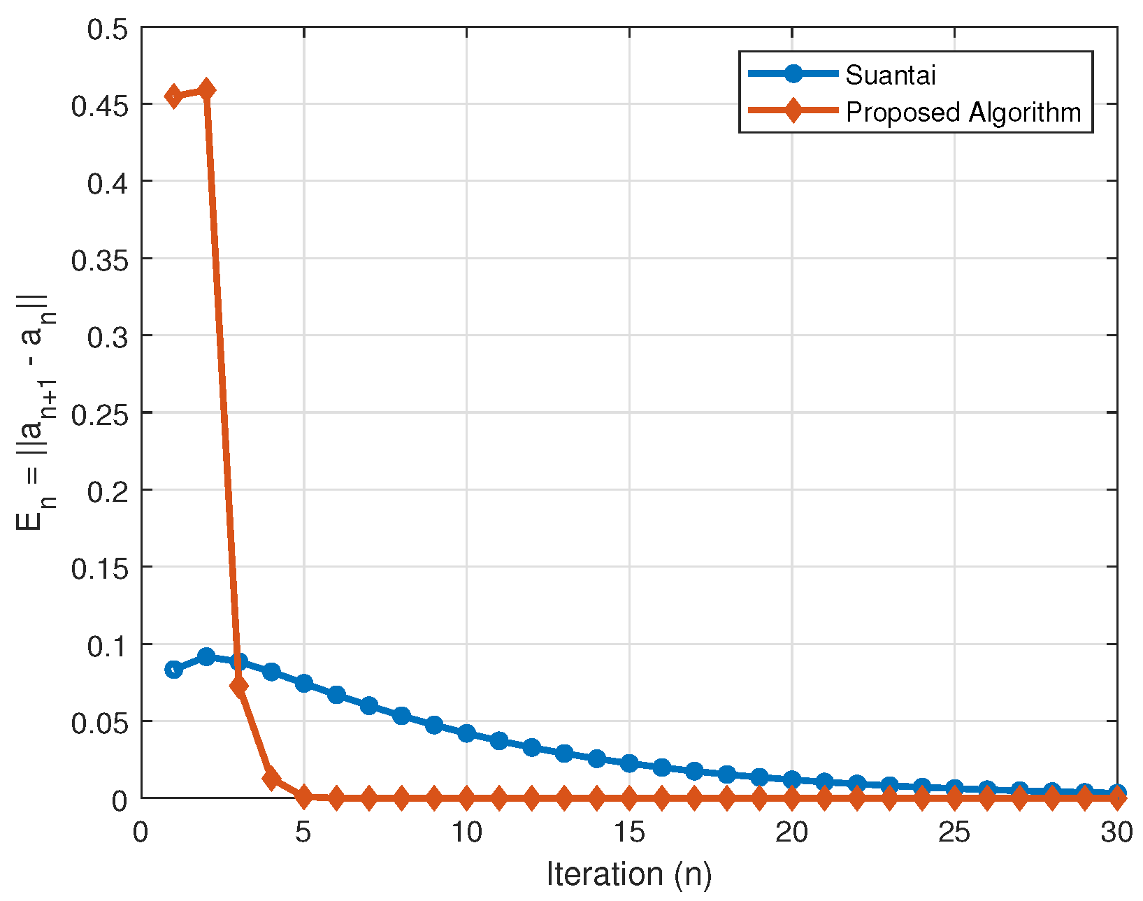
In Example 2, we compare convergence behavior and efficiency of our proposed Algorithm 6 with the comparable algorithm given in Equation (6) of Suantai [39] and the comparison can be seen in

Table 2. Numerical comparison for both algorithms.

No. Iter	Suantai [39]	${\mathit{E}}_{\mathit{n}}=\parallel {\mathit{a}}_{\mathit{n}+1}-{\mathit{a}}_{\mathit{n}}\parallel$	Proposed Algorithm	${\mathit{E}}_{\mathit{n}}=\parallel {\mathit{a}}_{\mathit{n}+1}-{\mathit{a}}_{\mathit{n}}\parallel$
0	(0, 1.0000)	–	(0, 1.0000)	–
1	(0, 0.916667)	0.0833333	(0, 1)	0.454861
2	(0, 0.825)	0.0916667	(0, 0.545139)	0.458831
3	(0, 0.736607)	0.0883929	(0, 0.0863084)	0.072751
4	(0, 0.654762)	0.0818452	(0, 0.0135574)	0.0126738
5	(0, 0.580357)	0.0744048	(0, 0.000883564)	0.000835067
6	(0, 0.513393)	0.0669643	(0, 4.84972 × 10−5)	4.67119 × 10−5
7	(0, 0.453497)	0.0598958	(0, 1.78533 × 10−6)	1.72936 × 10−6
8	(0, 0.400144)	0.0533526	(0, 5.59731 × 10−8)	5.4418 × 10−8
9	(0, 0.352759)	0.0473855	(0, 1.55506 × 10−9)	1.51619 × 10−9
10	(0, 0.310764)	0.0419951	(0, 3.88768 × 10−11)	3.79933 × 10−11
11	(0, 0.273607)	0.0371565	(0, 8.83564 × 10−13)	8.65157 × 10−13
12	(0, 0.240774)	0.0328329	(0, 1.84076 × 10−14)	1.80536 × 10−14
13	(0, 0.211792)	0.0289821	(0, 3.53992 × 10−16)	3.47671 × 10−16
14	(0, 0.186231)	0.0255611	(0, 6.32129 × 10−18)	6.21593 × 10−18
15	(0, 0.163703)	0.022528	(0, 1.05355 × 10−19)	1.03709 × 10−19
16	(0, 0.14386)	0.0198428	(0, 1.64617 × 10−21)	1.62196 × 10−21
17	(0, 0.126392)	0.0174688	(0, 2.42084 × 10−23)	2.38721 × 10−23
18	(0, 0.11102)	0.015372	(0, 3.36227 × 10−25)	3.31803 × 10−25
19	(0, 0.097498)	0.0135216	(0, 4.42404 × 10−27)	4.36874 × 10−27
20	(0, 0.085608)	0.01189	(0, 5.53005 × 10−29)	5.46422 × 10−29
21	(0, 0.0751559)	0.0104521	(0, 6.5834 × 10−31)	6.50859 × 10−31
22	(0, 0.0659702)	0.00918572	(0, 7.48113 × 10−33)	7.39982 × 10−33
23	(0, 0.0578994)	0.00807082	(0, 8.13167 × 10−35)	8.04696 × 10−35
24	(0, 0.0508096)	0.00708972	(0, 8.47049 × 10−37)	8.38578 × 10−37
25	(0, 0.044583)	0.00622667	(0, 8.47049 × 10−39)	8.38904 × 10−39
26	(0, 0.0391152)	0.00546772	(0, 8.1447 × 10−41)	8.06928 × 10−41
27	(0, 0.0343147)	0.00480051	(0, 7.54139 × 10−43)	7.47405 × 10−43
28	(0, 0.0301006)	0.00421409	(0, 6.73338 × 10−45)	6.67534 × 10−45
29	(0, 0.0264018)	0.00369881	(0, 5.80464 × 10−47)	5.75627 × 10−47
30	(0, 0.0231557)	0.00324613	(0, 4.8372 × 10−49)	4.79819 × 10−49
…	…	…	…	…
145	(0, 5.54148 × 10−9)	7.88532 × 10−10	(0, 0)	0
146	(0, 4.85116 × 10−9)	6.90321 × 10−10	(0, 0)	0
147	(0, 4.24682 × 10−9)	6.04339 × 10−10	(0, 0)	0
148	(0, 3.71775 × 10−9)	5.29065 × 10−10	(0, 0)	0
149	(0, 3.25459 × 10−9)	4.63165 × 10−10	(0, 0)	0
150	(0, 2.84912 × 10−9)	4.05472 × 10−10	(0, 0)	0

and Figure 2.

Example 2.

Suppose that ${\mathcal{H}}_1={\mathbb{R}}^2,{\mathcal{H}}_2=\mathbb{R}$ and $C_1=[-1,0]\times [0,1]$, $C_2=[3,7]\times [0,1]$, $C=[-3,0]$. Define $F:C\times C\to \mathbb{R}$ by $F(a,b)=(a-1)(b-a),\forall a,b\in C$. Set G as zero mapping and mapping $A:{\mathcal{H}}_1\to {\mathcal{H}}_2$ as $A(a,b)=3a,\forall (a,b)\in {\mathcal{H}}_1$ and $S:C_1\to C_2$ as $S(a,b)=\left(3-a,{\displaystyle \frac{b}{2}}\right),\forall (a,b)\in C_1,C_0=\{(0,b):0\le b\le 1\}$. Further, we set $r_n={\displaystyle \frac{n}{n+1}}$, $\tau ={\displaystyle \frac{1}{20}}, \Phi \left(a\right)={\displaystyle \frac{a}{4}}, {\delta }_n=0.5$, ${\eta }_n=0.5$, ${\alpha }_n={\displaystyle \frac{n}{2n+1}}$, ${\beta }_n={\displaystyle \frac{1}{2}}(1-{\alpha }_n)={\displaystyle \frac{3n+2}{4n+2}}$, and ${\gamma }_n=1-{\alpha }_n-{\beta }_n$, $\forall n\ge 1$.

Note that mapping F satisfies $\left(A_1\right)-\left(A_4\right)$ of Assumption A1 and $GEP(F,G)=\left\{0\right\}.$ Set $S=T$ which is the best proximally nonexpansive mapping with $S\left(C_0\right)\subseteq D_0\mathrm{and}\mathcal{B}\left(S\right)=\left\{(0,0)\right\}$.

Remark 5.

We take initial point $a_0=a_1=(0,1)$ in the comparison analysis. From Table 2, we observe that the sequence $\left\{a_n\right\}$ proposed in Algorithm 6 converges to $(0,0)$ which is a best proximity point of S. By Table 2 and Figure 2, our proposed algorithm converges faster than the algorithm defined in Equation (6) of Suantai and Tiammee [39].

Example 3.

Assume that ${\mathcal{H}}_1={\mathcal{H}}_2=R^3$ and $C_1=C_2=C=\{a\in R^3:\langle u,a\rangle \ge v\}$. Define the following: ${\mu }_n=3-{\displaystyle \frac{1}{3n-1}},{\eta }_n={\displaystyle \frac{n}{2n+1}},{\tau }_n={\displaystyle \frac{1}{3n+1}},r_n=1-{\displaystyle \frac{3}{n+3}}$, $\lambda ={\lambda }_1={\lambda }_2=0.55,{\delta }_n=0.8,{\beta }_n={\gamma }_n={\displaystyle \frac{2+n}{2n+5}},{\alpha }_n={\displaystyle \frac{1}{2n+7}}$, $\Phi \left(a\right)={\displaystyle \frac{a}{4}}$, $S\left(a\right)={\displaystyle \frac{a}{7}}$, $T\left(a\right)={\displaystyle \frac{a}{5}}$. Further, set $\sigma =0.0001$ in Algorithms 2 and 3, and $\eta =0.45$, $S=T$ in Algorithm 3.

$$L_1=\left(\begin{array}{ccc}7& 0& 0\\ 5& 5& 0\\ 0& 0& 2\end{array}\right),L_2=\left(\begin{array}{ccc}8& 0& 0\\ 0& 7& 0\\ 0& 0& 3\end{array}\right)A=\left(\begin{array}{ccc}6& 3& 1\\ 8& 7& 5\\ 3& 6& 2\end{array}\right)$$

For $r>0$, $G_r^F\left(a\right)={\displaystyle \frac{v-\langle u,a\rangle }{{\parallel a\parallel }^2}}u+a$. We fix $u=(7,-2,2)$ and $v=-1$ and select the different initial guesses with $Tol=\parallel a_{n+1}-a_n\parallel <{10}^{-3}$. We also present the error curves plotted against the number of iterations for each test case. The corresponding graphical results are shown in Figure 3.

Remark 6.

Observe Figure 3, where different initial guesses are tested and the corresponding errors are plotted against the number of iterations. From these results, we note that varying the starting points and parameters does not significantly affect the performance of our iterative scheme in terms of its convergence speed. Figure 3 clearly illustrates that the proposed algorithm performs efficiently and remains stable under different initial conditions.

4. Application to Image Restoration

Images play a crucial role in many areas such as engineering, medical diagnosis and security applications. In this experiment, we apply the proposed algorithm to restore images that have been corrupted by noise. For evaluation, Algorithm 6 is compared with Algorithms 2 and 3 on the image restoration task using MATLAB.

We examine the restored images, and compared to the corresponding signal-to-noise ratio (SNR) values, it becomes evident that the proposed algorithm performs well than the other methods considered in this study.

We recall the split linear inverse problem introduced in [44]:

$$\mathrm{Find}{a}^{*}\in {\mathcal{H}}_1\mathrm{such}\mathrm{that}\mathcal{P}\left(a^{*}\right)+\mathcal{Q}\left(a^{*}\right)=\underset{a\in {\mathcal{H}}_1}{min}[\mathcal{P}\left(a\right)+\mathcal{Q}\left(a\right)],$$

(37)

where $\mathcal{P}:{\mathcal{H}}_1\to$ is convex and continuously differentiable and $\mathcal{Q}:{\mathcal{H}}_1\to \mathbb{R}$ is convex and lower semicontinuous.

A commonly studied special case of (37) is the image restoration model, written as follows:

$$\underset{a\in {\mathbb{R}}^n}{min}\left\{{\parallel La-b\parallel }_2^2+\lambda {\parallel a\parallel }_1\right\},$$

(38)

where $\lambda >0$, $a\in {\mathbb{R}}^n$ represents the original image, $b\in {\mathbb{R}}^m$ is the noisy image and $L:{\mathbb{R}}^n\to {\mathbb{R}}^m$ is a linear (blurring) operator. In this setting, we consider $\mathcal{P}\left(a\right)={\parallel La-b\parallel }_2^2$ and $\mathcal{Q}\left(a\right)={\lambda \parallel a\parallel }_1$.

The function $\mathcal{P}$ is convex and continuously differentiable, and its gradient $\nabla \mathcal{P}$ is monotone and continuous. Since $\mathcal{Q}$ is convex and lower semicontinuous, its subdifferential $\partial \mathcal{Q}$ is maximal monotone. Therefore, Problem (37) becomes equivalent to the following monotone inclusion:

$$\mathcal{P}\left(a^{*}\right)+\mathcal{Q}\left(a^{*}\right)=\underset{a\in {\mathcal{H}}_1}{min}[\mathcal{P}\left(a\right)+\mathcal{Q}\left(a\right)]\iff 0\in \left(\nabla \mathcal{P}\left(a^{*}\right)+\partial \mathcal{Q}\left(a^{*}\right)\right),$$

(39)

where $\nabla \mathcal{P}$ is monotone and Lipschitz continuous with Lipschitz constant ${\parallel L\parallel }^2$. If we choose $L_1=\nabla \mathcal{P}+\partial \mathcal{Q}$, $L_2=0$, $A=0$ and $C_1=C_2$ in algorithms, then the generated sequence $\left\{a_n\right\}$ converges strongly to the solution of the monotone inclusion problem stated in (39).

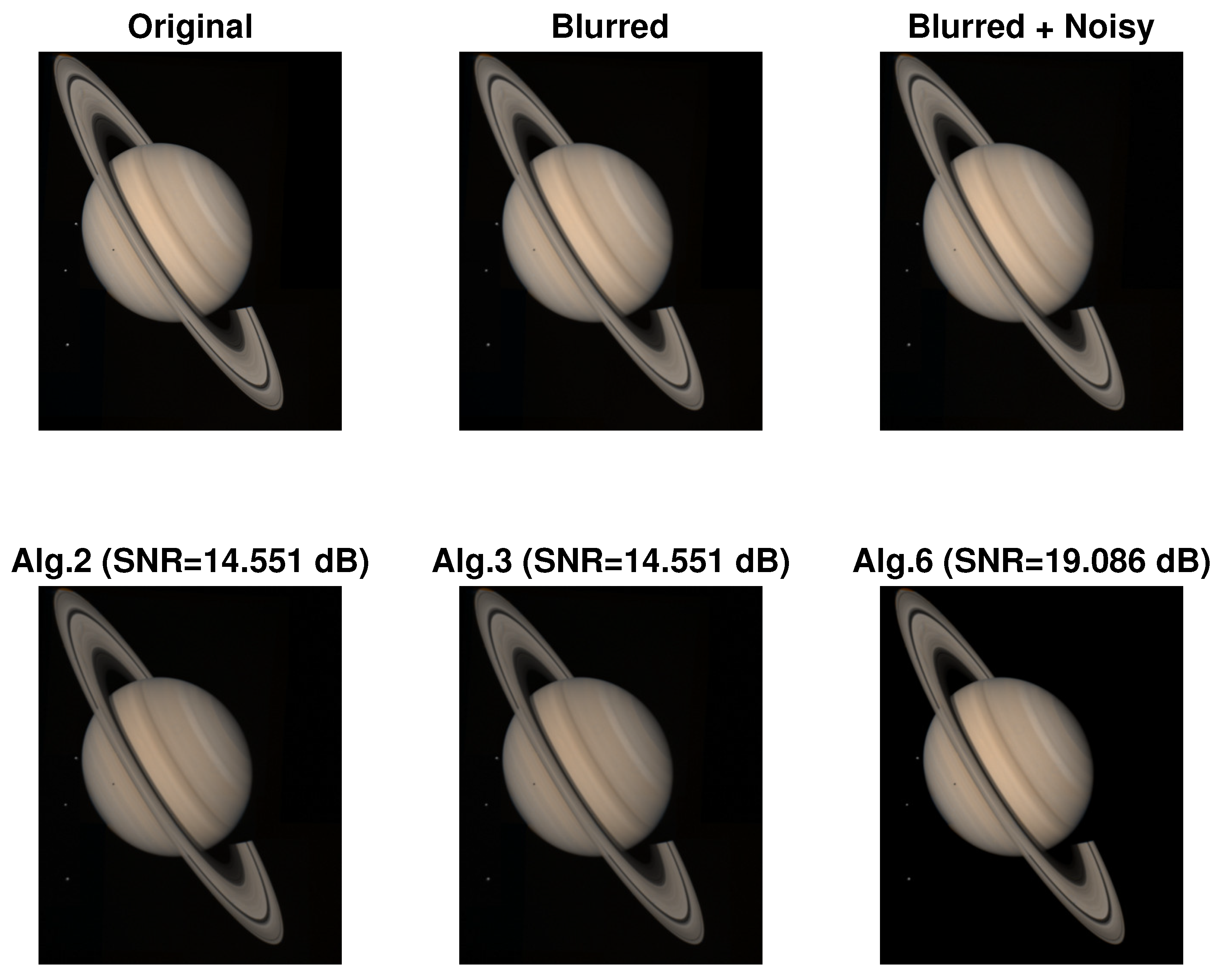
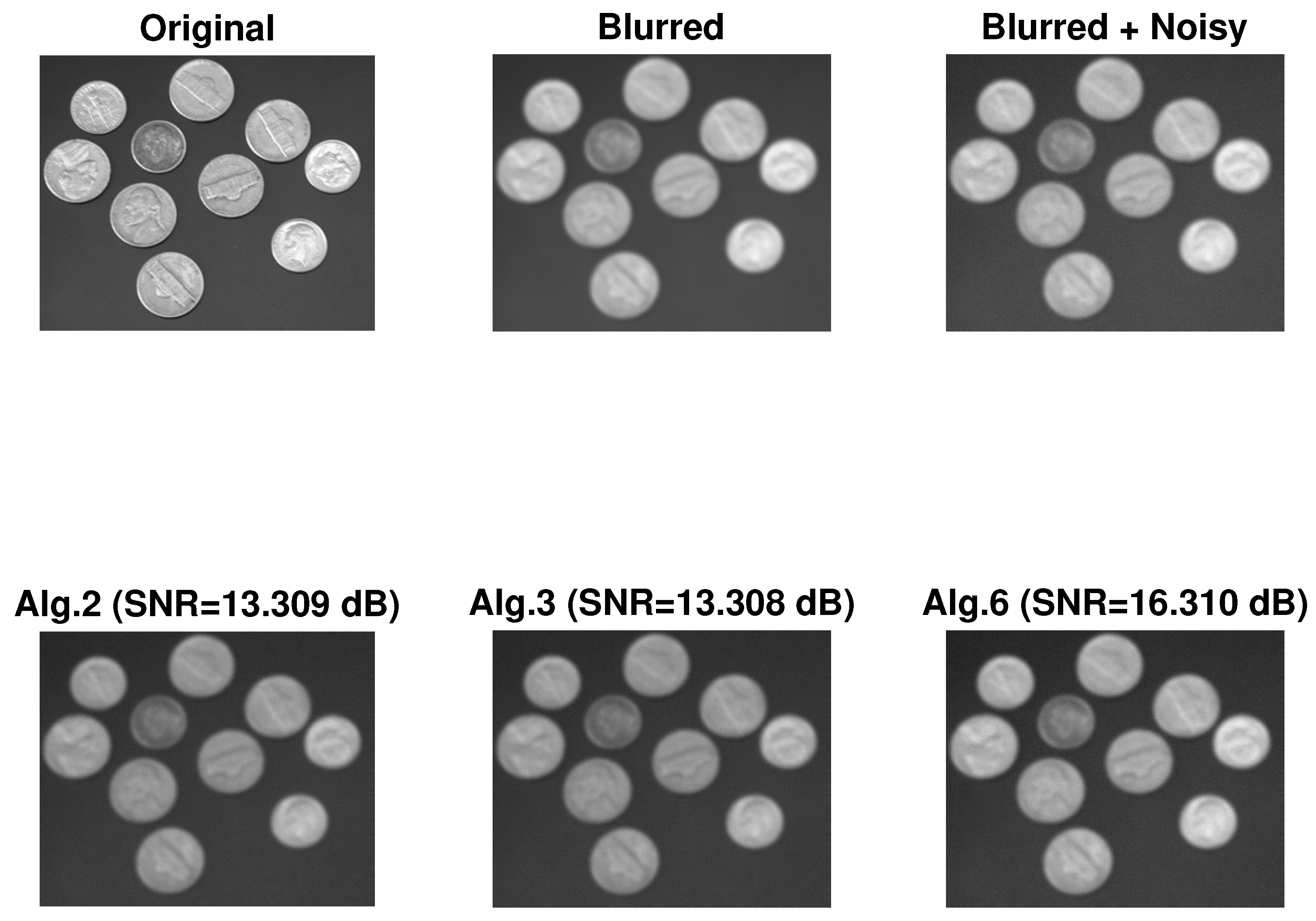
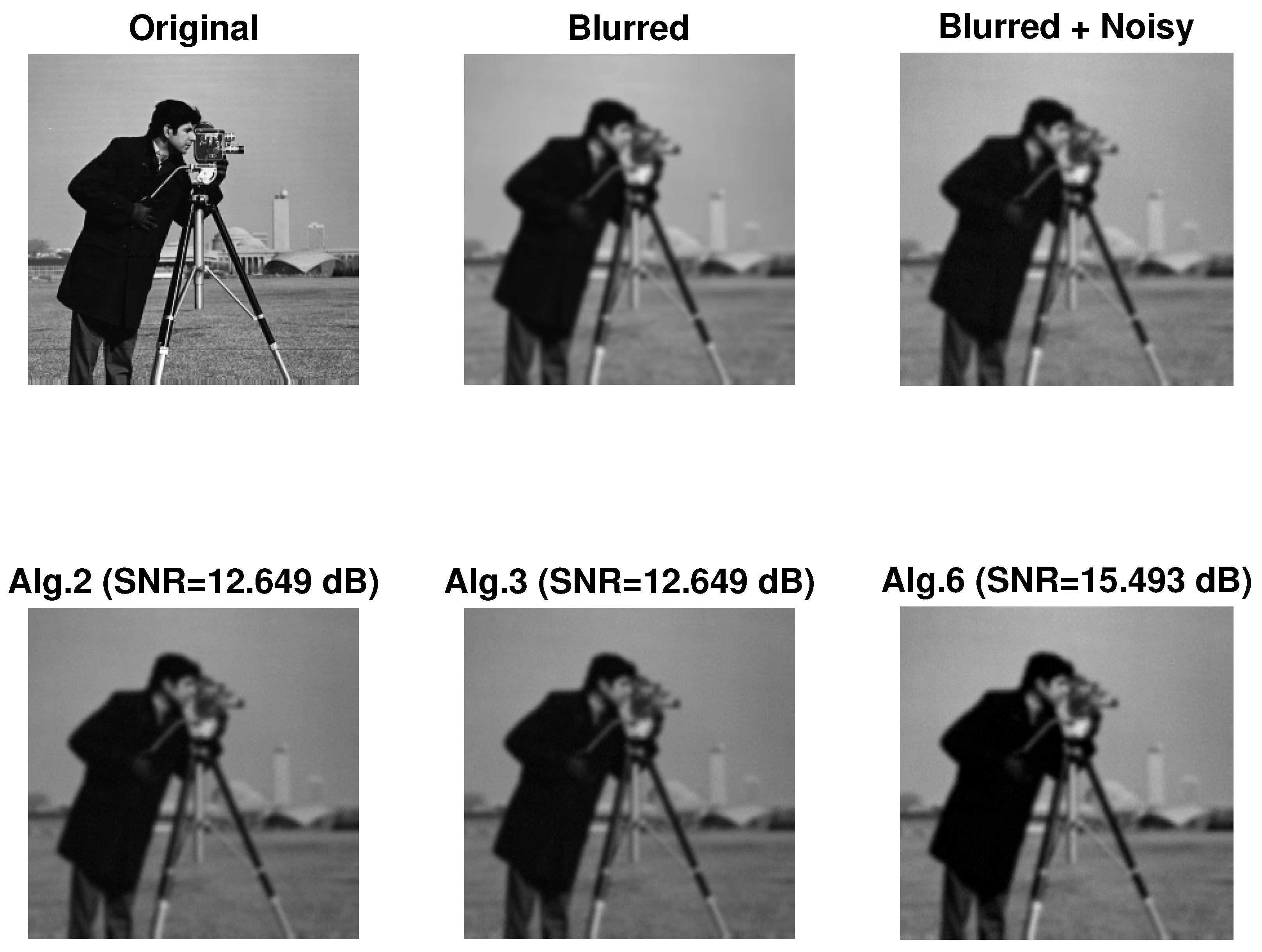
For the numerical evaluation, we select several color and grayscale images from a standard benchmark dataset. In the control parameters, we use a blur kernel with standard deviation $\sigma =2$, Gaussian kernel size 9, Gaussian noise level $0.01$, and set $\lambda ={\lambda }_1=0.55$, ${\eta }_n=0.75$, with a maximum of 30 iterations. To assess the quality of the restored images, we use both visual inspection and the signal-to-noise ratio (SNR), expressed in decibels (dB) and defined by

$$\mathrm{SNR}=20\times {log}_{10}\left({\displaystyle \frac{\parallel a\parallel }{\parallel a-a_r\parallel }}\right),$$

where a denotes the original image and $a_r$ is the reconstructed (deblurred) image. A higher SNR value indicates better reconstruction performance. The restored results for the color images are displayed in Figure 4, Figure 5, Figure 6 and Figure 7.

Remark 7.

Observe Figure 4, Figure 5, Figure 6 and Figure 7. Algorithm 6 performs better than Algorithms 2 and 3: it yields higher SNR values in the image restoration experiments for both color and grayscale images which confirms its practical advantage for denoising and deblurring tasks.

5. Conclusions and Future Work

In this paper, we approximate the common solution of common best proximity point, split variational inclusion and generalized equilibrium problem using inertial type iterative algorithm. The main features of our paper are: (1) The step size in the algorithms proposed in [39,40,42] requires prior knowledge of the operator norm, whereas our proposed algorithm involves self-adaptive step size. (2) The strong convergence result of the proposed Algorithm 6 is proved. (3) Approximation of a common solution of three nonlinear problems is obtained instead of finding their solutions separately. (4) In view of Remarks 4 and 7, our approach is more efficient and converges faster than the algorithms proposed in [39,40]. In future research, we may extend our self-adaptive inertial scheme to non-convex models and large-scale imaging problems requiring distributed computation. We may also apply our main algorithm to solve compressed sensing problems.

References

1. Bauschke, H.H.; Borwein, J.M. On projection algorithms for solving convex feasibility problems. SIAM Rev. 1996, 38, 367–426. [Google Scholar] [CrossRef]
2. Chen, P.; Huang, J.; Zhang, X. A primal–dual fixed point algorithm for convex separable minimization with applications to image restoration. Inverse Probl. 2013, 29, 025011. [Google Scholar] [CrossRef]
3. Goebel, K.; Reich, S. Uniform Convexity, Hyperbolic Geometry, and Non-Expansive Mappings; CRC Press: Boca Raton, FL, USA, 1984. [Google Scholar]
4. Deutsch, F. Best Approximation in Inner Product Spaces; Springer: Berlin/Heidelberg, Germany, 2001; Volume 7. [Google Scholar]
5. Zhao, J.; Liang, Y.; Liu, Y.; Cho, Y.J. Split equilibrium, variational inequality and fixed point problems for multi-valued mappings in Hilbert spaces. Appl. Comput. Math 2018, 17, 271–283. [Google Scholar]
6. Agarwal, R.P.; O’Regan, D.; Sahu, D.R. Fixed Point Theory for Lipschitzian-Type Mappings with Applications; Springer: Berlin/Heidelberg, Germany, 2009; Volume 6. [Google Scholar]
7. Chuang, C.-S. Strong convergence theorems for the split variational inclusion problem in Hilbert spaces. Fixed Point Theory Appl. 2013, 2013, 350. [Google Scholar] [CrossRef]
8. Osilike, M.O.; Igbokwe, D.I. Weak and strong convergence theorems for fixed points of pseudocontractions and solutions of monotone type operator equations. Comput. Math. Appl. 2000, 40, 559–567. [Google Scholar] [CrossRef]
9. Maing, P.-E. Approximation methods for common fixed points of nonexpansive mappings in Hilbert spaces. J. Math. Anal. Appl. 2007, 325, 469–479. [Google Scholar] [CrossRef]
10. Saejung, S.; Yotkaew, P. Approximation of zeros of inverse strongly monotone operators in Banach spaces. Nonlinear Anal. 2012, 75, 742–750. [Google Scholar] [CrossRef]
11. Barbagallo, A. Existence and regularity of solutions to nonlinear degen-erate evolutionary variational inequalities with applications to dynamic network equilibrium problems. Appl. Math. Comput. 2009, 208, 1–13. [Google Scholar]
12. Dafermos, S.; Nagurney, A. A network formulation of market equilibrium problems and variational inequalities. Oper. Res. Lett. 1984, 3, 247–250. [Google Scholar] [CrossRef]
13. He, R. Coincidence theorem and existence theorems of solutions for a system of Ky Fan type minimax inequalities in FC-spaces. Adv. Fixed Point Theory 2012, 2, 47–57. [Google Scholar]
14. Qin, X.; Cho, S.Y.; Kang, S.M. Strong convergence of shrinking projection methods for quasi-ϕ-nonexpansive mappings and equilibrium problems. J. Comput. Appl. Math. 2010, 234, 750–760. [Google Scholar] [CrossRef]
15. Sadiq Basha, S. Best proximity points: Optimal solutions. J. Optim. Theory Appl. 2011, 151, 210–216. [Google Scholar] [CrossRef]
16. Sadiq Basha, S. Best proximity points: Global optimal approximate solutions. J. Glob. Optim. 2011, 49, 15–21. [Google Scholar] [CrossRef]
17. Gabeleh, M. Best proximity point theorems via proximal non-self mappings. J. Optim. Theory Appl. 2015, 164, 565–576. [Google Scholar] [CrossRef]
18. Suparatulatorn, R.; Suantai, S. A new hybrid algorithm for global mini-mization of best proximity points in Hilbert spaces. Carpath. J. Math. 2019, 35, 95–102. [Google Scholar] [CrossRef]
19. Bunlue, N.; Suantai, S. Hybrid algorithm for common best proximity points of some generalized nonself nonexpansive mappings. Math. Methods Appl. Sci. 2018, 41, 7655–7666. [Google Scholar] [CrossRef]
20. Moussaoui, A.; Park, C.; Melliani, S. New best proximity point results via simulation functions in fuzzy metric spaces. Bol. Soc. Paran. Mat. 2025, 43, 1–12. [Google Scholar]
21. Husain, S.; Furkan, M.; Khairoowala, M.U. Strong convergence of inertial shrinking projection method for split best proximity point problem and mixed equilibrium problem. J. Anal. 2025, 33, 31–48. [Google Scholar] [CrossRef]
22. Byrne, C. Iterative oblique projection onto convex sets and the split feasibility problem. Inverse Probl. 2002, 18, 441. [Google Scholar] [CrossRef]
23. Combettes, P.L. The convex feasibility problem in image recovery. Adv. Imaging Electron Phys. 1996, 95, 155–270. [Google Scholar]
24. Censor, Y.; Gibali, A.; Reich, S. Algorithms for the split variational inequality problem. Numer. Algorithms 2012, 59, 301–323. [Google Scholar] [CrossRef]
25. Tang, Y. Convergence analysis of a new iterative algorithm for solving split variational inclusion problems. J. Ind. Manag. Optim. 2020, 16, 945–964. [Google Scholar] [CrossRef]
26. Raj, V.S. Best proximity point theorems for non-self mappings. Fixed Point Theory 2013, 14, 447–454. [Google Scholar]
27. Halpern, B. Fixed points of nonexpanding maps. Bull. Am. Math. Soc. 1976, 73, 959. [Google Scholar] [CrossRef]
28. Iiduka, H. Fixed point optimization algorithm and its application to network bandwidth allocation. J. Comput. Appl. Math. 2012, 236, 1733–1742. [Google Scholar] [CrossRef]
29. Kazmi, K.R.; Rizvi, S.H. An iterative method for split variational inclusion problem and fixed point problem for a nonexpansive mapping. Optim. Lett. 2014, 8, 1113–1124. [Google Scholar] [CrossRef]
30. Moudafi, A. Viscosity approximation methods for fixed-points problems. J. Math. Anal. Appl. 2000, 241, 46–55. [Google Scholar] [CrossRef]
31. Asghar, M.W.; Abbas, M. A self-adaptive viscosity algorithm for split fixed point problems and variational inequality problems in Banach spaces. J. Non. Con. Anal. 2023, 24, 341–361. [Google Scholar]
32. Abbas, M.; Asghar, M.W.; De la Sen, M. Approximation of the solution of delay fractional differential equation using AA-iterative scheme. Mathematics 2022, 10, 273. [Google Scholar] [CrossRef]
33. Asghar, M.W.; Abbas, M.; Eyni, D.C.; Omaba, M.E. Iterative approximation of fixed points of generalized αm-nonexpansive mappings in modular spaces. AIMS Math. 2023, 8, 26922–26944. [Google Scholar] [CrossRef]
34. Suanoom, C.; Gebrie, A.G.; Grace, T. The convergence of AA-iterative algorithm for generalized AK-α-nonexpansive mappings in Banach spaces. Sci. Technol. Asia 2023, 28, 82–90. [Google Scholar]
35. Beg, I.; Abbas, M.; Asghar, M.W. Convergence of AA-iterative algorithm for generalized α-nonexpansive mappings with an application. Mathematics 2022, 10, 4375. [Google Scholar] [CrossRef]
36. Abbas, M.; Ciobanescu, C.; Asghar, M.W.; Omame, A. Solution approximation of fractional boundary value problems and convergence analysis using AA-iterative scheme. AIMS Math. 2024, 9, 13129–13158. [Google Scholar] [CrossRef]
37. Byrne, C.; Censor, Y.; Gibali, A.; Reich, S. The split common null point problem. J. Nonlinear Convex Anal. 2012, 13, 759–775. [Google Scholar]
38. Wangkeeree, R.; Rattanaseeha, K.; Wangkeeree, R. The general iterative methods for split variational inclusion problem and fixed point problem in Hilbert spaces. J. Comput. Anal. Appl 2018, 25, 19–31. [Google Scholar]
39. Suantai, S.; Tiammee, J. The shrinking projection method for solving split best proximity point and equilibrium problems. Filomat 2021, 35, 1133–1140. [Google Scholar] [CrossRef]
40. Husain, S.; Khan, F.A.; Furkan, M.; Khairoowala, M.U.; Eljaneid, N.H. Inertial projection algorithm for solving split best proximity point and mixed equilibrium problems in Hilbert spaces. Axioms 2022, 11, 321. [Google Scholar] [CrossRef]
41. Asghar, M.W.; Abbas, M.; Rouhani, B.D. The AA-Viscosity Algorithm for Fixed-Point, Generalized Equilibrium and Variational Inclusion Problems. Axioms 2024, 13, 38. [Google Scholar] [CrossRef]
42. Sharma, S.; Chandok, S. Split fixed point problems for quasi-nonexpansive map-pings in Hilbert spaces. Politehn. Univ. Bucharest Sci. Bull. Ser. A Appl. Math. Phys. 2024, 86, 109–118. [Google Scholar]
43. Aubin, J.-P. Optima and Equilibria: An Introduction to Nonlinear Analysis; Springer Science Business Media: Berlin/Heidelberg, Germany, 2002; Volume 140. [Google Scholar]
44. Beck, A.; Teboulle, M. A fast iterative shrinkage-thresholding algorithm for linear inverse problems. SIAM J. Imaging Sci. 2009, 2, 183–202. [Google Scholar] [CrossRef]
Figure 1. Comparison of Husain et al. [40] and the proposed algorithm.
Axioms 14 00924 g001
Figure 2. Error plot: Comparison of Suantai [39] and the proposed algorithm.
Axioms 14 00924 g002
Figure 3. Error analysis plots for different initial values. (a) a 0 = ( 5 , 2.2 , 3.45 ) , a 1 = ( 5 , 1.25 , 3.2 ) . (b) a 0 = ( 6.25 , 2.12 , 3.45 ) , a 1 = ( 4 , 1.45 , 3 ) . (c) a 0 = ( 3.56 , 2.67 , 4.35 ) , a 1 = ( 5.75 , 0.62 , 1.22 ) . (d) a 0 = ( 24 , 11.7 , 33.5 ) , a 1 = ( 15.5 , 8.45 , 20 ) .
Axioms 14 00924 g003
Figure 4. Image restoration results for Saturn.
Axioms 14 00924 g004
Figure 5. Image restoration results for Peppers.
Axioms 14 00924 g005
Figure 6. Image restoration results for Coins.
Axioms 14 00924 g006
Figure 7. Image restoration results for Cameraman.
Axioms 14 00924 g007