On a Queuing Model with Customers Arriving According to a Diffusion Process

Abstract

In the case of heavy traffic, the arrival process in a queuing model can be approximated by a diffusion process. In this paper, we consider such a model. The number $X\left(t\right)$ of customers in the system at time t evolves according to a degenerate two-dimensional diffusion process. In a special case, the distribution of $X\left(t\right)$ is calculated explicitly. Moreover, a stochastic control problem known as a homing problem is formulated, and the equation satisfied by the value function is given. Particular homing problems are solved explicitly.

1. Introduction

Queuing theory originated from the pioneering work of Danish engineer Agner Krarup Erlang. In the early 20th century, he developed the first mathematical models to answer questions related to the number of telephone lines and operators needed to satisfy a random demand; see refs. [1,2]. Since then, this theory has become an important subject in many fields, notably in operations research, telecommunications, and computer system design.

Seminal works on queuing theory include the papers by Khinchine [3], Kendall [4], and Jackson [5]. Khinchine obtained a formula that characterizes the waiting-time and queue-length distributions in the M/G/1 queue, which is one of the most fundamental results in queuing theory. In his paper, Kendall proposed the notation (such as M/M/1, M/G/1) that is widely used to classify queuing systems. Jackson showed that under the assumptions of Poisson arrivals and exponential service times, the stationary distribution of open queuing networks factorizes into a product of independent node distributions.

Finally, classic books on this subject include the monographs by Cox and Smith [6] and Kleinrock [7].

In classical queuing models, the arrivals of customers constitute a discrete-space stochastic process. For instance, in the case of the $M/M/s$ model, where s is the number of servers, customers arrive according to a Poisson process. However, in some applications, arrivals occur almost according to a diffusion process. This is true, in particular, in the case of heavy traffic (for instance, on the Internet). See, for example, Lee et al. [8] and Lee and Weerasingheb [9].

In this paper, which is a vastly expanded version of the conference paper [10], we assume that the number $X\left(t\right)$ of customers in the system at time t is such that

$$\begin{array}{ccc}\hfill \mathrm{d}X\left(t\right)& =& \rho \left[X\right(t),Y(t\left)\right]\mathrm{d}t-kX\left(t\right)\mathrm{d}t,\hfill \end{array}$$

(1)

$$\begin{array}{ccc}\hfill \mathrm{d}Y\left(t\right)& =& m\left[Y\left(t\right)\right]\mathrm{d}t+{\left\{v\left[Y\left(t\right)\right]\right\}}^{1/2}\mathrm{d}B\left(t\right),\hfill \end{array}$$

(2)

where $\left\{B\right(t),t\ge 0\}$ is a one-dimensional standard Brownian motion. The functions $m(·)\in \mathbb{R}$ and $v(·)>0$ are such that $\left\{Y\right(t),t\ge 0\}$ is a diffusion process. Moreover, the non-negative constant k is the rate at which the customers are served. The function $\rho (·,·)$ should be such that if $k=0$, then $X\left(t\right)$ will increase with time t.

This type of degenerate two-dimensional diffusion process, which was proposed by Rishel [11], has been used in reliability theory to model the wear of devices. Indeed, wear should be strictly increasing with time. If we want to model the remaining lifetime instead, then it should be decreasing with time. In ref. [11], the model introduced is in fact in multidimensional. Furthermore, the infinitesimal parameters of the process $\left\{Y\right(t),t\ge 0\}$ may depend on $X\left(t\right)$. Thus, Equation (2) can be replaced by

$$\mathrm{d}{Y}_i\left(t\right)=m[X\left(t\right),Y_i\left(t\right)]\mathrm{d}t+{\left\{v[X\left(t\right),Y_i\left(t\right)]\right\}}^{1/2}\mathrm{d}{B}_i\left(t\right),$$

(3)

for $i=1,\dots ,n$.

Remark 1.

(i) With this type of model, in which the variations in the number of customers in the system is approximated by a diffusion process, there is no individual service time distribution as such. We see that if $\rho \left(X\right(t),Y(t\left)\right)\equiv 0$ in Equation (1), then $X\left(t\right)\propto e^{-kt}$. Hence the statement that the constant k is the service rate of customers. (ii) Several authors have used a diffusion process as an approximation of the variations in $X\left(t\right)$. A commonly used model is reflected Brownian motion (see, for instance, refs. [12,13]), so that the number of customers cannot become negative. With the model that we propose, this result can be guaranteed without having to introduce a reflective barrier. (iii) To implement the proposed model, we must first identify the process $\left\{Y\right(t),t\ge 0\}$ on which the variations in $X\left(t\right)$ depend. In the case of the application to reliability theory, $Y\left(t\right)$ can be an environmental variable, such as temperature or the speed at which the machine is used. Here, $Y\left(t\right)$ could be the market share of a company at time t. This share varies due, in particular, to competition between companies. The variable $Y\left(t\right)$ could also be the pool of all potential customers for the company. This pool may increase or decrease, depending on the activities of the company we are interested in, for example by opening branches in new countries or closing others. Next, we would need to estimate the infinitesimal parameters (that is, $m(·)$ and $v(·)$) of $\left\{Y\right(t),t\ge 0\}$. Finally, we would also need to estimate the function $\rho (·,·)$ and the constant k using real data.

In the next section, a particular case for the various functions in Equations (1) and (2) will be considered. Then, in Section 3, an optimal control problem for the two-dimensional process $\left\{\right(X\left(t\right),Y\left(t\right)),t\ge 0\}$ will be studied. In Section 4, explicit and exact solutions to particular cases of this control problem will be presented. Finally, some concluding remarks will end this paper in Section 5.

2. A Particular Case

Suppose that $m(·)\equiv \mu >0$ and $v(·)\equiv {\sigma }^2$ in Equation (2). Then, $\left\{Y\right(t),t\ge 0\}$ is a Wiener process with positive drift $\mu$ and dispersion parameter $\sigma >0$. A Wiener process, being a Gaussian process, can take both positive and negative values. Therefore, the function $\rho (·,·)$ should be such that $\rho \left[X\right(t),Y(t\left)\right]$ is a non-negative function. For example, we could take $\rho [X\left(t\right),Y\left(t\right)]=Y^2\left(t\right)$. However, if we assume that $y:=Y\left(0\right)$ and $\mu$ are both large enough, and that $\sigma$ is small, then the probability that $Y\left(t\right)$ becomes negative is negligible.

We choose $\rho \left[X\right(t),Y(t\left)\right]=cY\left(t\right)$, with c being a positive constant. With this choice, we can appeal to the following proposition to compute the joint probability density function of the random vector $\left(X\right(t),Y(t\left)\right)$.

Proposition 1

([14]). Let $\left\{\mathbf{X}\right(t),t\ge 0\}$ be an n-dimensional stochastic process defined by

$$d\mathbf{X}\left(t\right)=(\mathbf{A}\mathbf{X}\left(t\right)+\mathbf{a})\mathrm{d}t+{\mathbf{N}}^{1/2}\mathrm{d}\mathbf{B}\left(t\right),$$

(4)

where $\left\{\mathbf{B}\right(t),t\ge 0\}$ is an n-dimensional standard Brownian motion, $\mathbf{A}$ is a square matrix of order n, $\mathbf{a}$ is an n-dimensional vector, and ${\mathbf{N}}^{1/2}$ is a positive definite square matrix of order n. Then, given that $\mathbf{X}\left(t_0\right)=\mathbf{x}$, we may write that

$$\mathbf{X}\left(t\right)\sim \mathrm{N}\left(\mathbf{m}\left(t\right),\mathbf{K}\left(t\right)\right)for t\ge t_0,$$

(5)

where

$$\mathbf{m}\left(t\right):=\mathbf{\Phi }\left(t\right)\left(\mathbf{x}+{\int }_{t_0}^t{\mathbf{\Phi }}^{-1}\left(u\right)\mathbf{a}\mathrm{d}u\right)$$

(6)

and

$$\mathbf{K}\left(t\right):=\mathbf{\Phi }\left(t\right)\left({\int }_{t_0}^t{\mathbf{\Phi }}^{-1}\left(u\right)\mathbf{N}{\left[{\mathbf{\Phi }}^{-1}\left(u\right)\right]}^{\prime }\mathrm{d}u\right){\mathbf{\Phi }}^{\prime }\left(t\right),$$

(7)

where the symbol prime denotes the transpose of the matrix, and the function $\mathbf{\Phi }\left(t\right)$ is given by

$$\mathbf{\Phi }\left(t\right):=e^{\mathbf{A}(t-t_0)}=\sum _{n=0}^{\infty }{\mathbf{A}}^n{\displaystyle \frac{{(t-t_0)}^n}{n!}}.$$

(8)

Remark 2.

In words, the above proposition tells us that any affine transformation of an n-dimensional standard Brownian motion (which is a Gaussian process) remains a Gaussian process. Moreover, it provides the formulas needed to compute the mean and the covariance function of the new process.

In our case, we have

$$\mathbf{A}=\left[\begin{array}{cc}-k& c\\ 0& 0\end{array}\right],\mathbf{a}=\left[\begin{array}{c}0\\ \mu \end{array}\right]\mathrm{and}{\mathbf{N}}^{1/2}=\left[\begin{array}{cc}0& 0\\ 0& \sigma \end{array}\right].$$

(9)

The coefficient matrix $\mathbf{A}$ contains the service rate k and the constant c. We chose $\rho \left[X\right(t),Y(t\left)\right]=cY\left(t\right)$; that is, the value of $X^{\prime }\left(t\right)$ is assumed to increase at a rate which is proportional to $Y\left(t\right)$ (if $k=0$), and c is the constant of proportionality. We also assumed that $\left\{Y\right(t),t\ge 0\}$ is a Wiener process with infinitesimal parameters $\mu$ and $\sigma$. The vector $\mathbf{a}$ contains the drift $\mu$, and $\sigma$ appears in the degenerate constant matrix $\mathbf{N}$, which is the noise matrix.

Now, for $n\ge 1$,

$${\mathbf{A}}^n=\left[\begin{array}{cc}{(-k)}^n& -c{(-k)}^{n-1}\\ 0& 0\end{array}\right].$$

(10)

Hence, if $t_0=0$, the function $\mathbf{\Phi }\left(t\right)$ is given by

$$\begin{array}{ccc}\hfill \mathbf{\Phi }\left(t\right)& =& \left[\begin{array}{cc}1& 0\\ 0& 1\end{array}\right]+\left[\begin{array}{cc}-1+e^{-kt}& -{\displaystyle \frac{c}{k}}\left(-1+e^{-kt}\right)\\ 0& 0\end{array}\right]\hfill \\ & =& \left[\begin{array}{cc}{e}^{-kt}& -{\displaystyle \frac{c}{k}}\left(-1+e^{-kt}\right)\\ 0& 1\end{array}\right].\hfill \end{array}$$

(11)

Next, we find that

$${\int }_0^t{\mathbf{\Phi }}^{-1}\left(u\right)\mathbf{a}\mathrm{d}u=\left[\begin{array}{c}{\displaystyle \frac{c\mu \left(-kt-1+{\mathit{e}}^{kt}\right)}{k^2}}\\ \mu t\end{array}\right].$$

(12)

It follows that

$$\mathbf{m}\left(t\right)=\left[\begin{array}{c}{\mathit{e}}^{-kt}\left(x+{\displaystyle \frac{c\mu \left(-kt-1+{\mathit{e}}^{kt}\right)}{k^2}}\right)-{\displaystyle \frac{c\left({\mathit{e}}^{-kt}-1\right)\left(\mu t+y\right)}{k}}\\ \mu t+y\end{array}\right].$$

(13)

Finally, with

$$\mathbf{N}=\left[\begin{array}{cc}0& 0\\ 0& {\sigma }^2\end{array}\right],$$

(14)

we calculate

$${\int }_0^t{\mathbf{\Phi }}^{-1}\left(u\right)\mathbf{N}{\left[{\mathbf{\Phi }}^{-1}\left(u\right)\right]}^{\prime }\mathrm{d}u=\left[\begin{array}{cc}-{\displaystyle \frac{c^2{\sigma }^2\left(-2kt+4{\mathit{e}}^{kt}-{\mathit{e}}^{2kt}-3\right)}{2k^3}}& -{\displaystyle \frac{c{\sigma }^2\left(-kt-1+{\mathit{e}}^{kt}\right)}{k^2}}\\ -{\displaystyle \frac{c{\sigma }^2\left(-kt-1+{\mathit{e}}^{kt}\right)}{k^2}}& {\sigma }^{2}t\end{array}\right]$$

(15)

and

$$\mathbf{K}\left(t\right)=\left[\begin{array}{cc}{\displaystyle \frac{c^2{\sigma }^2\left(2{\mathit{e}}^{2kt}kt-3{\mathit{e}}^{2kt}+4{\mathit{e}}^{kt}-1\right){\mathit{e}}^{-2kt}}{2k^3}}& {\displaystyle \frac{c{\sigma }^2\left(kt-1+{\mathit{e}}^{-kt}\right)}{k^2}}\\ {\displaystyle \frac{c{\sigma }^2\left(kt-1+{\mathit{e}}^{-kt}\right)}{k^2}}& {\sigma }^{2}t\end{array}\right].$$

(16)

Notice that for t large, $X\left(t\right)$ has a Gaussian distribution with mean and variance that are both (approximately) affine functions of t.

Making use of the above results, we can compute the probability that $X\left(t\right)$ will become equal to zero, so that the queue is empty, as a function of time. Similarly, if the system capacity is finite, we can easily compute the probability that the system will become saturated.

The actual (approximate) number of customers in the system is given by

$$X_r\left(t\right):=\left\{\begin{array}{cc}0& \mathrm{if}X\left(t\right)\le 0,\hfill \\ X\left(t\right)& \mathrm{if}0<X\left(t\right)<r,\hfill \\ r& \mathrm{if}X\left(t\right)\ge r,\hfill \end{array}\right.$$

(17)

where r is the system capacity.

Corollary 1.

Suppose that the system (1), (2) is of the form

$$\begin{array}{ccc}\hfill \mathrm{d}X\left(t\right)& =& cln\left[Y\right(t\left)\right]\mathrm{d}t-kX\left(t\right)\mathrm{d}t,\hfill \end{array}$$

(18)

$$\begin{array}{ccc}\hfill \hspace{1em}\hspace{1em}\hspace{1em}\hspace{1em}\hspace{1em}\hspace{1em} \mathrm{d}Y\left(t\right)& =& \left(\mu +{\displaystyle \frac{1}{2}}{\sigma }^2\right)Y\left(t\right)\mathrm{d}t+{\left\{{\sigma }^2{Y}^2\left(t\right)\right\}}^{1/2}\mathrm{d}B\left(t\right),\hfill \end{array}$$

(19)

where $c>0$, $\mu \in \mathbb{R}$ and $\sigma >0$. Then $X\left(t\right)$ has a Gaussian distribution with mean and variance given by

$$E\left[X\left(t\right)\right]={\mathit{e}}^{-kt}\left(x+{\displaystyle \frac{c\mu \left(-kt-1+{\mathit{e}}^{kt}\right)}{k^2}}\right)-{\displaystyle \frac{c\left({\mathit{e}}^{-kt}-1\right)\left(\mu t+y\right)}{k}}$$

(20)

and

$$\mathrm{VAR}\left[X\left(t\right)\right]={\displaystyle \frac{c^2{\sigma }^2\left(2{\mathit{e}}^{2kt}kt-3{\mathit{e}}^{2kt}+4{\mathit{e}}^{kt}-1\right){\mathit{e}}^{-2kt}}{2k^3}}.$$

(21)

Proof. 

The diffusion process $\left\{Y\right(t),t\ge 0\}$ is a geometric Brownian motion with infinitesimal mean $\left(\mu +{\displaystyle \frac{1}{2}}{\sigma }^2\right)y$ and infinitesimal variance ${\sigma }^2{y}^2$. A geometric Brownian motion is non-negative (if it starts at $Y\left(0\right)=y>0$), since it can be expressed as the exponential of a Wiener process. If we define $Z\left(t\right)=ln\left[Y\right(t\left)\right]$, then $\left\{Z\right(t),t\ge 0\}$ is a Wiener process with infinitesimal mean $\mu$ and infinitesimal variance ${\sigma }^2$. The results are then deduced at once from Proposition 1. □

Remark 3.

We assume that both $Y\left(0\right)=y$ and the parameter μ are large enough (and σ small enough) for the probability $P\left[Y\right(t)<1]$ to be negligible.

Next, assume that the system (1), (2) is

$$\begin{array}{ccc}\hfill \mathrm{d}X\left(t\right)& =& cY\left(t\right)\mathrm{d}t-kX\left(t\right)\mathrm{d}t,\hfill \end{array}$$

(22)

$$\begin{array}{ccc}\hfill \hspace{1em}\hspace{1em}\hspace{1em}\hspace{1em}\hspace{1em}\mathrm{d}Y\left(t\right)& =& m_{0}Y\left(t\right)\mathrm{d}t+{\left\{v_0{Y}^2\left(t\right)\right\}}^{1/2}\mathrm{d}B\left(t\right),\hfill \end{array}$$

(23)

where $m_0\in \mathbb{R}$ and $v_0>0$. Then, $X\left(t\right)$ will not have a Gaussian distribution. We can at least compute its expected value.

Proposition 2.

The expected value of the random variable $X\left(t\right)$ in the system (22), (23) is

$$E\left[X\left(t\right)\right]=\left({\displaystyle \frac{2cy\left({\mathit{e}}^{(v_0/2)t+m_{0}t+kt}-1\right)}{v_0+2k+2\mu }}+\mathit{x}\right){\mathit{e}}^{-kt},$$

(24)

where $x=X\left(0\right)$ and $y=Y\left(0\right)$.

Proof. 

The solution of the ordinary differential equation (ODE)

$$X^{\prime }\left(t\right)=cY\left(t\right)-kX\left(t\right)$$

(25)

that satisfies the initial condition $X\left(0\right)=x$ is

$$X\left(t\right)=\left({\int }_0^{t}cY\left(w\right){\mathit{e}}^{kw}\mathrm{d}w+\mathit{x}\right){\mathit{e}}^{-kt}.$$

(26)

Moreover, we have

$$E\left[Y\left(t\right)\right]=yexp\left\{\left(m_0+{\displaystyle \frac{v_0}{2}}\right)t\right\}.$$

(27)

The expected value of $X\left(t\right)$ is then obtained by computing

$$E\left[X\left(t\right)\right]=\left({\int }_0^{t}cyexp\left\{\left(m_0+{\displaystyle \frac{v_0}{2}}\right)w\right\}{\mathit{e}}^{kw}\mathrm{d}w+\mathit{x}\right){\mathit{e}}^{-kt}.$$

(28)

□

Remark 4.

In the special case when $m_0=-v_0/2$, so that $E\left[Y\right(t\left)\right]\equiv y$, we have

$$\underset{t\to \infty }{lim}E\left[X\left(t\right)\right]={\displaystyle \frac{cy}{k}}.$$

(29)

In the next section, an optimal control problem for the two-dimensional stochastic process $\left(X\right(t),Y(t\left)\right)$ will be examined.

3. A Homing Problem

In this section, we suppose that the term $kX\left(t\right)$ in Equation (1) is replaced by the function $b\left[X\right(t),Y(t\left)\right]u\left[X\right(t),Y(t\left)\right]$, where $b(·,·)$ is a non-negative function and $u(·,·)$ is a control variable that is assumed to be a continuous function.

Let

$$\tau (x,y):=inf\{t>0:(X\left(t\right),Y\left(t\right))\in D\subset {\mathbb{R}}^2\mid X\left(0\right)=x,Y\left(0\right)=y,(x,y)\notin D\}.$$

(30)

The random variable $\tau (x,y)$ is called a first-passage time in probability theory.

Our aim is to find the control that minimizes the expected value of the cost functional

$$J(x,y):={\int }_0^{\tau (x,y)}\left\{{\displaystyle \frac{1}{2}}q[X\left(t\right),Y\left(t\right)]u^2[X\left(t\right),Y\left(t\right)]+\theta \right\}\mathrm{d}t+K[X\left(\tau (x,y)\right),Y\left(\tau (x,y)\right)],$$

(31)

where $q(·,·)>0$, $\theta \in \mathbb{R}$, and $K(·,·)$ is the final cost function. This type of stochastic control problem, in which a stochastic process is controlled until a given event occurs, is known as a homing problem; see Whittle [15]. The author of the current paper has written several articles on homing problems; see, for example, ref. [16]. Other papers on this subject are refs. [11,17].

Many papers have been published on the optimal control of queuing systems. Sometimes the authors assume that it is possible to control the service rate and/or the arrival rate of customers into the system.

In ref. [18], Laxmi and Jyothsna considered a discrete-time queue. Their objective was to minimize costs by optimizing the service rates. To do so, they used swarm optimization. In Tian et al. [19], the authors also treated a problem for a queuing system with varying service rates. Other papers in which the authors assumed that the service rate could be controlled are refs. [20,21,22,23,24]. In Wu et al. [25], the aim was rather to control customer arrivals. The main difference between these papers and the work presented here is that in our case the final time is a random variable. See Lefebvre and Yaghoubi [26] for other references on the optimal control of queuing systems.

To find the optimal control $u^{*}[X\left(t\right),Y\left(t\right)]$, we can try using dynamic programming, which enables us to express $u^{*}$ in terms of the value function

$$F(x,y):=\underset{\begin{array}{c}u\left[X\right(t),Y(t\left)\right]\\ t\in [0,\tau (x,y\left)\right)\end{array}}{inf}E\left[J(x,y)\right].$$

(32)

The function $F(x,y)$ gives the smallest expected cost (or largest expected reward, if the cost is negative), starting form $X\left(0\right)=x$ and $Y\left(0\right)=y$.

Using the results in ref. [15], we can state the following proposition.

Proposition 3.

The value function $F(x,y)$ satisfies the dynamic programming equation

$$\begin{array}{ccc}\hfill 0=\underset{\begin{array}{c}u(x,y)\end{array}}{inf}& & \{{\displaystyle \frac{1}{2}}q(x,y)u^2(x,y)+\theta +[\rho (x,y)-b(x,y)u(x,y)]F_x(x,y)\hfill \\ & & +m\left(y\right)F_y(x,y)+{\displaystyle \frac{1}{2}}v\left(y\right)F_{yy}(x,y)\},\hfill \end{array}$$

(33)

where $F_x(x,y)={\displaystyle \frac{\partial }{\partial x}}F(x,y)$, etc. The equation is valid for $(x,y)\notin D$. We have the boundary condition $F(x,y)=K(x,y)$ if $(x,y)\in D$. Moreover, the optimal control is given by

$$u^{*}(x,y)={\displaystyle \frac{b(x,y)}{q(x,y)}}{F}_x(x,y).$$

(34)

If we substitute the expression for $u^{*}(x,y)$ into the dynamic programming equation, we find that to obtain the value function, we must solve the second-order non-linear partial differential equation (PDE)

$$\theta -{\displaystyle \frac{b^2(x,y)}{2q(x,y)}}{\left[F_x(x,y)\right]}^2+\rho (x,y)F_x(x,y)+m\left(y\right)F_y(x,y)+{\displaystyle \frac{1}{2}}v\left(y\right)F_{yy}(x,y)=0.$$

(35)

Assume now that instead of the service rate, the optimizer can control the arrival rate of the process, so that the two-dimensional process $\left(X\right(t),Y(t\left)\right)$ is defined by the system of stochastic differential equations

$$\begin{array}{ccc}\hfill \mathrm{d}X\left(t\right)& =& \rho \left[X\right(t),Y(t\left)\right]\mathrm{d}t-kX\left(t\right)\mathrm{d}t,\hspace{1em}\hspace{1em}\hspace{1em}\hspace{1em}\hspace{1em}\hspace{1em}\hspace{1em}\hspace{1em}\hspace{1em}\hspace{1em}\hspace{1em}\hspace{1em}\hspace{1em}\hfill \end{array}$$

(36)

$$\begin{array}{ccc}\hfill \hspace{1em}\hspace{1em}\mathrm{d}Y\left(t\right)& =& b[X\left(t\right),Y\left(t\right)]u[X\left(t\right),Y\left(t\right)]\mathrm{d}t+m\left[Y\left(t\right)\right]\mathrm{d}t+{\left\{v\left[Y\left(t\right)\right]\right\}}^{1/2}\mathrm{d}B\left(t\right).\hfill \end{array}$$

(37)

Proceeding as above, we obtain the following corollary.

Corollary 2.

In the case of the controlled process defined in Equations (36) and (37), the optimal control is given by

$$u^{*}(x,y)=-{\displaystyle \frac{b(x,y)}{q(x,y)}}{F}_y(x,y).$$

(38)

Furthermore, the value function satisfies the PDE

$$0=\theta -{\displaystyle \frac{b^2(x,y)}{2q(x,y)}}{\left[F_x(x,y)\right]}^2+[\rho (x,y)-kx]F_x(x,y)+m\left(y\right)F_y(x,y)+{\displaystyle \frac{1}{2}}v\left(y\right)F_{yy}(x,y).$$

(39)

Finally, in some cases, Equation (39) (as well as Equation (35)) can be linearized.

Proposition 4.

Suppose that there exists a positive constant α such that

$$\alpha ={\displaystyle \frac{b^2(x,y)}{q(x,y)v\left(y\right)}}.$$

(40)

Then the function

$$G(x,y):=e^{-\alpha F(x,y)}$$

(41)

satisfies the linear second-order PDE

$$\alpha \theta G(x,y)=[\rho (x,y)-kx]G_x(x,y)+m\left(y\right)G_y(x,y)+{\displaystyle \frac{1}{2}}{\sigma }^2{G}_{yy}(x,y).$$

(42)

The boundary condition is $G(x,y)=e^{-\alpha K(x,y)}$ if $(x,y)\in D$.

Remark 5.

The linear PDE in Equation (42) is in fact the Kolmogorov backward equation satisfied by the moment-generating function of the random variable $\tau (x,y)$:

$$M(x,y):=E\left[e^{-\omega \tau (x,y)}\right],$$

(43)

with $\omega :=\alpha \theta >0$, for the uncontrolled process $(X_0\left(t\right),Y_0\left(t\right))$ obtained by setting $u\left[X\right(t),Y(t\left)\right]\equiv 0$ in Equation (37). Moreover, the boundary condition is the appropriate one, and we assume that $P\left[\tau \right(x,y)<\infty ]=1$ for the uncontrolled process.

In the next section, explicit solutions to particular homing problems will be presented.

4. Explicit Solutions

Problem I.

The first particular homing problem that we consider is the one for which the function $\rho \left[X\right(t),Y(t\left)\right]$ in Equation (1) is equal to $cY\left(t\right)$, where c is a positive constant, and the term $kX\left(t\right)$ is replaced by $b_{0}u[X\left(t\right),Y\left(t\right)]$, with $b_0>0$. Moreover, we take

$$q[X\left(t\right),Y\left(t\right)]={\displaystyle \frac{q_0}{X^2\left(t\right)}},$$

(44)

where $q_0>0$, and we define the first-passage time

$$\tau (x,y)=inf\left\{t>0:{\displaystyle \frac{Y\left(t\right)}{X\left(t\right)}}=k_1\mathrm{or}{k}_2|X\left(0\right)=x,Y\left(0\right)=y,0<k_1<{\displaystyle \frac{y}{x}}<k_2\right\},$$

(45)

in which $\left\{Y\right(t),t\ge 0\}$ is a geometric Brownian motion that satisfies the stochastic differential Equation (23).

We assume that $\theta =0$ in Equation (31) and that the final cost is

$$K[X\left(\tau (x,y)\right),Y\left(\tau (x,y)\right)]=K_i\mathrm{if}{\displaystyle \frac{Y\left(\tau \right(x,y\left)\right)}{X\left(\tau \right(x,y\left)\right)}=k_i},\mathrm{for}i=1,2.$$

(46)

To obtain the value function, we must solve the PDE

$$-{\displaystyle \frac{b^2(x,y)}{2q(x,y)}}{\left[F_x(x,y)\right]}^2+cy{F}_x(x,y)+m_{0}y{F}_y(x,y)+{\displaystyle \frac{1}{2}}{v}_0{y}^2{F}_{yy}(x,y)=0,$$

(47)

subject to the boundary conditions $F(x,y)=K_i$ if $y/x=k_i$, for $i=1,2$.

Now, based on the boundary conditions, we look for a solution of the form

$$F(x,y)=H\left(z\right)\mathrm{with}z:=y/x.$$

(48)

This is an application of the method of similarity solutions. We find that Equation (47) is transformed into the non-linear second-order ODE

$$-{\displaystyle \frac{1}{2}}{\displaystyle \frac{b_0^2}{q_0}}{z}^2{\left[H^{\prime }\left(z\right)\right]}^2-c{z}^2{H}^{\prime }\left(z\right)+m_{0}z{H}^{\prime }\left(z\right)+{\displaystyle \frac{1}{2}}{v}_0{z}^2{H}^{″}\left(z\right)=0.$$

(49)

Next,

$$\beta :={\displaystyle \frac{q_0{v}_0}{b_0^2}}$$

(50)

is a positive constant. We set

$$\mathbf{\Psi }\left(z\right):=e^{-H\left(z\right)/\beta }.$$

(51)

We find that, if $m_0=0$, then the function $\mathbf{\Psi }\left(z\right)$ satisfies the simple linear ODE

$$c{\mathbf{\Psi }}^{\prime }\left(z\right)-{\displaystyle \frac{1}{2}}{v}_0{\mathbf{\Psi }}^{″}\left(z\right)=0,$$

(52)

whose general solution is

$$\mathbf{\Psi }\left(z\right)=c_1+c_2{e}^{2cz/v_0}.$$

(53)

The constants $c_1$ and $c_2$ are such that the boundary conditions $\mathbf{\Psi }\left(z\right)=e^{-K_i/\beta }$ if $z=k_i$, for $i=1,2$, are satisfied. We find that

$$\mathbf{\Psi }\left(z\right)={\displaystyle \frac{-{\mathit{e}}^{\frac{2cz\beta -{\mathit{K}}_{\mathit{2}}{v}_0}{v_0\beta }}+{\mathit{e}}^{\frac{2cz\beta -{\mathit{K}}_{\mathit{1}}{v}_0}{v_0\beta }}+{\mathit{e}}^{\frac{2c{\mathit{k}}_{\mathit{1}}\beta -{\mathit{K}}_{\mathit{2}}{v}_0}{v_0\beta }}-{\mathit{e}}^{\frac{2c{\mathit{k}}_{\mathit{2}}\beta -{\mathit{K}}_{\mathit{1}}{v}_0}{v_0\beta }}}{{\mathit{e}}^{\frac{2c{\mathit{k}}_{\mathit{1}}}{v_0}}-{\mathit{e}}^{\frac{2c{\mathit{k}}_{\mathit{2}}}{v_0}}}}$$

(54)

for $k_1\le z\le k_2$.

From the function $\mathbf{\Psi }\left(z\right)$, we obtain the value function $F(x,y)=H\left(z\right)=-\beta ln\left[\mathbf{\Psi }\right(z\left)\right]$, and hence the optimal control (see Equation (34))

$$u^{*}(x,y)={\displaystyle \frac{b_0{x}^2}{q_0}}{F}_x(x,y).$$

(55)

To illustrate the results, let us set $c=b_0=q_0=v_0=1$, $k_1=1$, $k_2=2$, $K_1=0$ and $K_2=1$. The constant $\beta$ is equal to 1, and we calculate

$$\mathbf{\Psi }\left(z\right)={\displaystyle \frac{e^{2z-1}-e^{2z}+e^4-e}{e^4-e^2}}$$

(56)

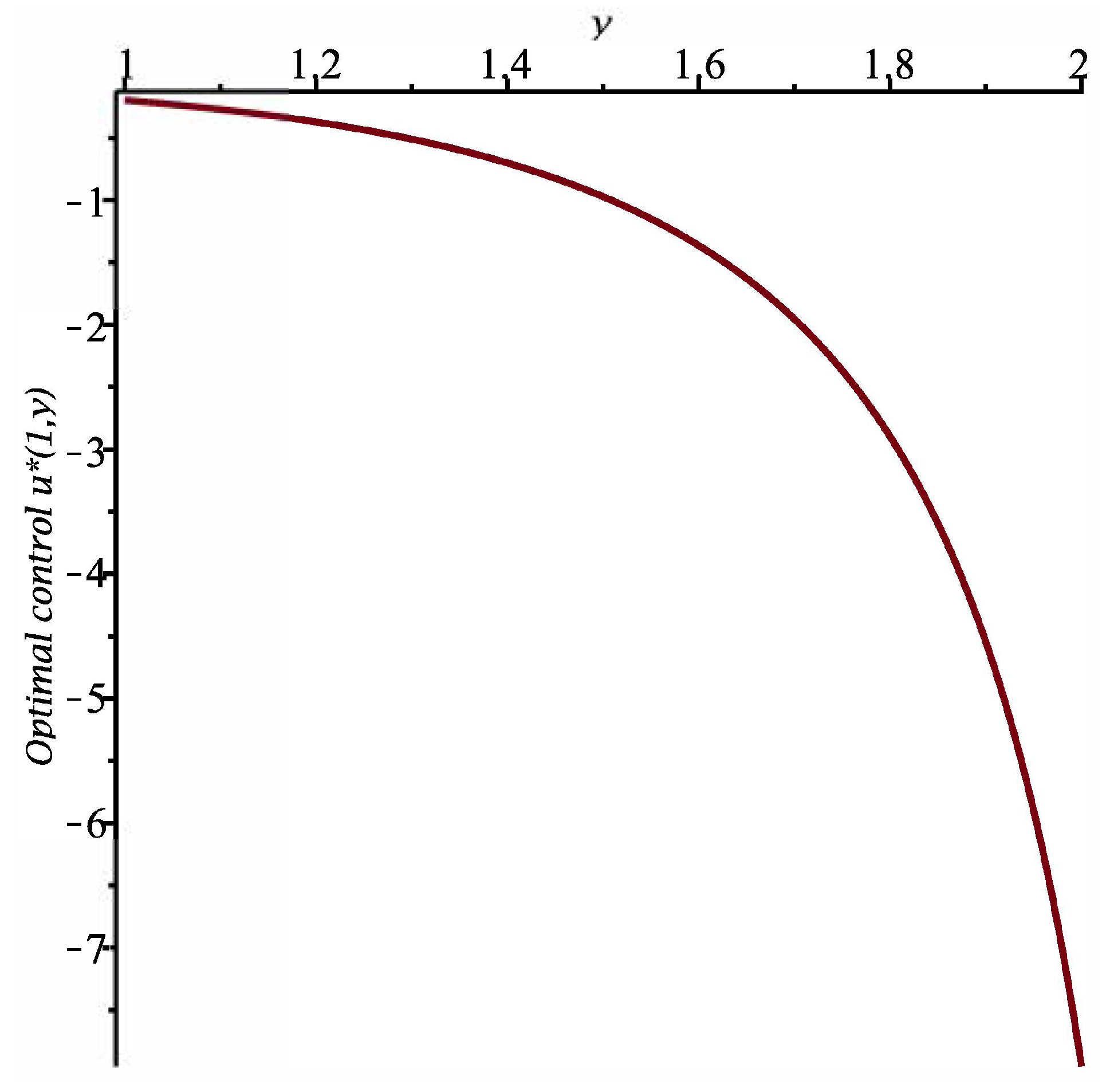
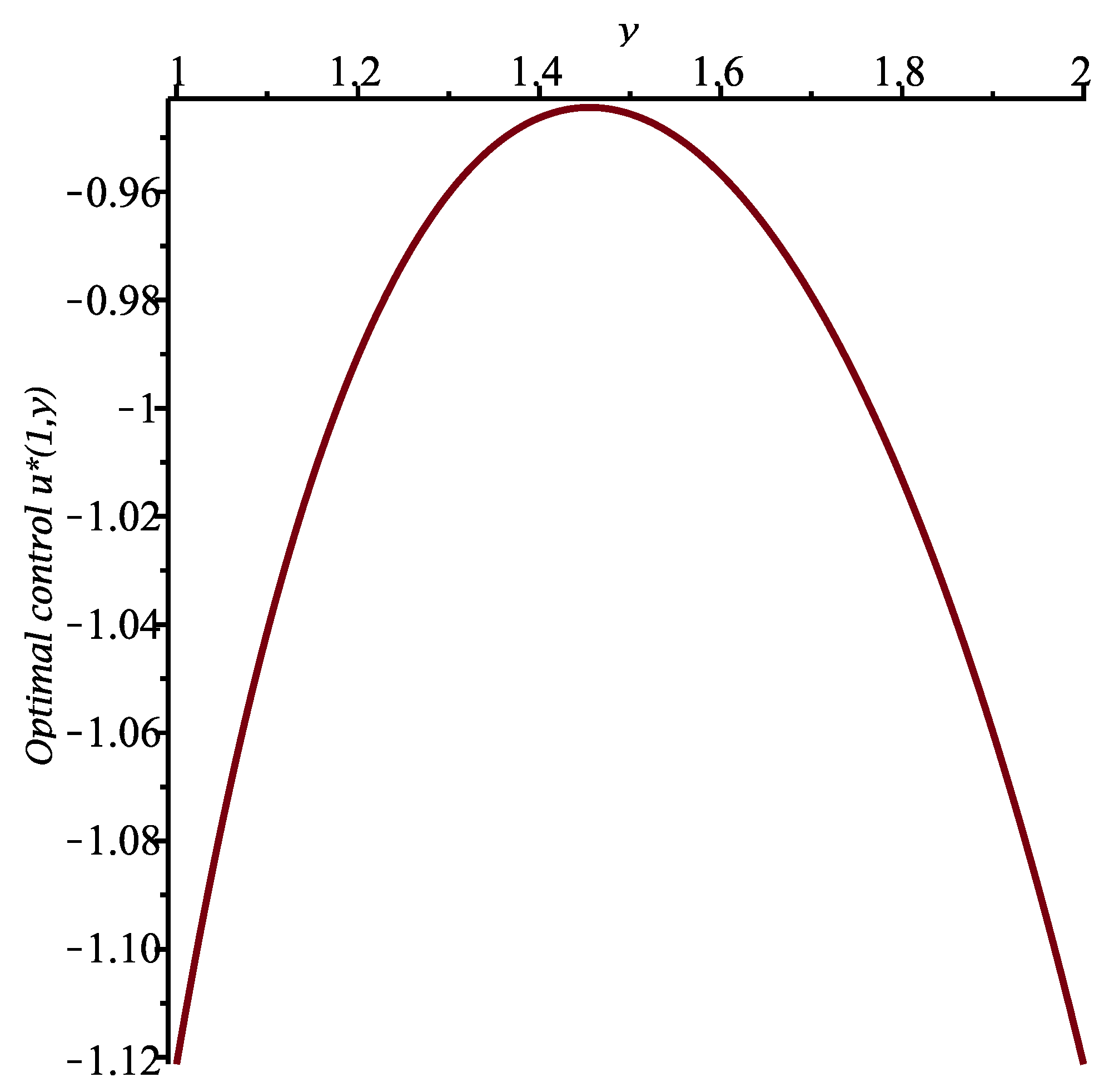
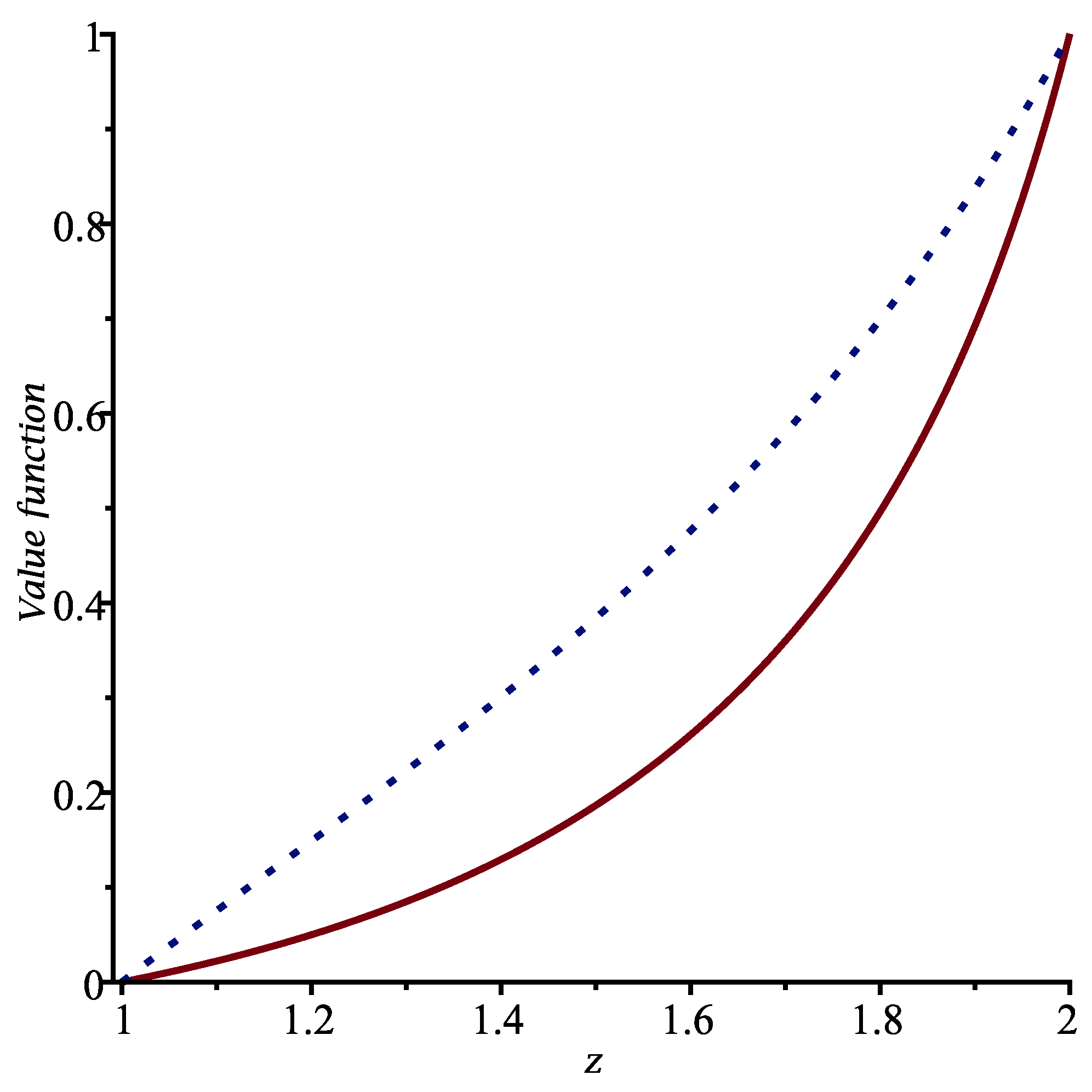
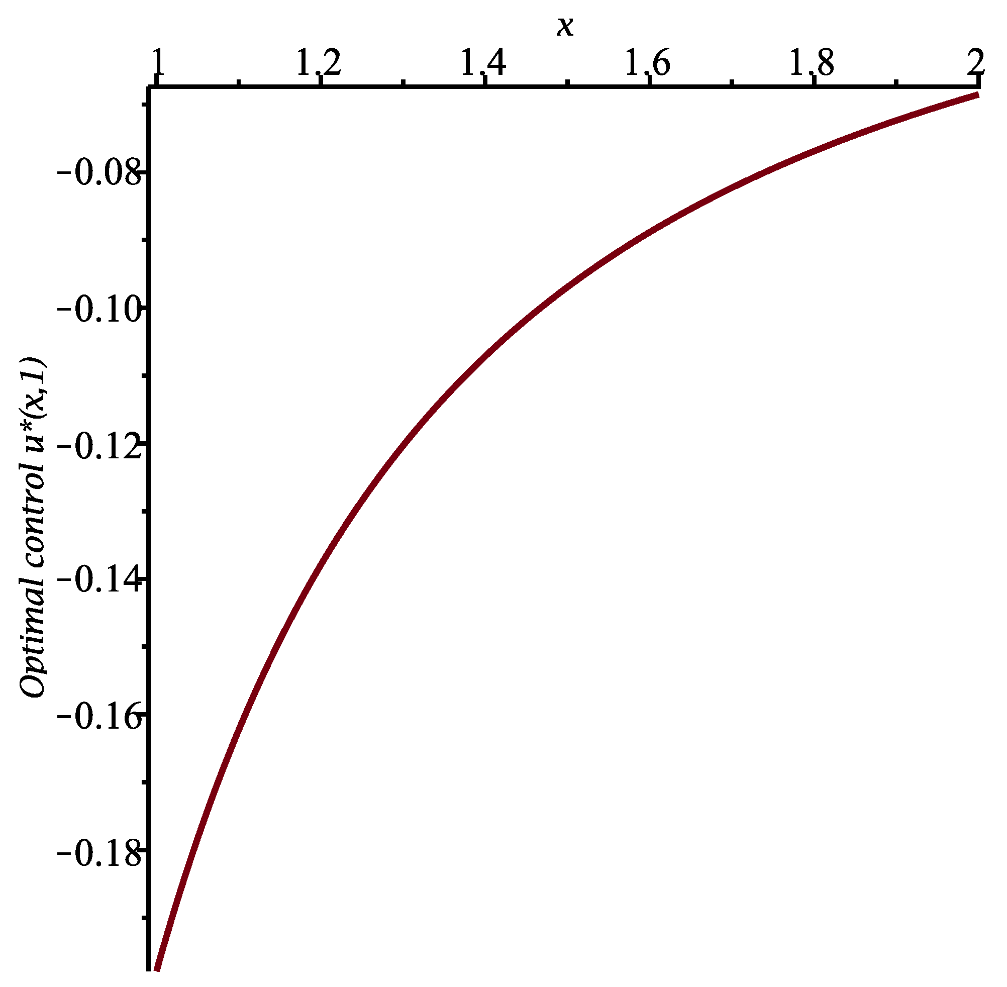
for $1\le z\le 2$. The function $H\left(z\right)$ is presented in Figure 1. Moreover, the optimal control $u^{*}(x,1)$ for $x\in [1,2]$ and $u^{*}(1,y)$ for $y\in [1,2]$ are shown in Figure 2 and Figure 3, respectively.

Remark 6.

Let $F_0(x,y)$ denote the expected cost if one uses no control. We have

$$F_0(x,y)=E[K[X\left(\tau (x,y)\right),Y\left(\tau (x,y)\right)].$$

(57)

This function satisfies the partial differential equation

$${\displaystyle \frac{1}{2}}{v}_0{y}^2{\displaystyle \frac{{\partial }^2{F}_0(x,y)}{\partial y^2}}+m_{0}y{\displaystyle \frac{\partial F_0(x,y)}{\partial y}}+cy{\displaystyle \frac{\partial F_0(x,y)}{\partial x}}=-1.$$

(58)

The boundary conditions are $F_0(x,y)=K_i$ if $y/x=k_i$, for $i=1,2$.

Let us look for a solution of the form $F_0(x,y)=H_0(z:=y/x)$. We find that we must solve the ODE

$${\displaystyle \frac{1}{2}}{v}_0{z}^2{H}_0^{″}\left(z\right)+(m_{0}z-c{z}^2)H_0^{\prime }\left(z\right)=-1.$$

(59)

With $m_0=0$ (as above), the general solution of Equation (59) is

$$H_0\left(z\right)=\int -{\displaystyle \frac{4{\mathit{e}}^{2z}{\mathit{Ei}}_{\mathit{1}}\left(2z\right)z-{\mathit{e}}^{2z}{\mathit{c}}_{\mathit{1}}z-2}{z}}\mathrm{d}z+{\mathit{c}}_{\mathit{2}},$$

(60)

where $E{i}_1(·)$ is an exponential integral function. With the same choices for the various constants as above, the particular solution that satisfies the boundary conditions $H_0\left(1\right)=0$ and $H_0\left(2\right)=1$ can be expressed as follows:

$$H_0\left(z\right)={\int }_1^z-{\displaystyle \frac{4{\mathit{e}}^{2\mathit{w}}{\mathit{Ei}}_{\mathit{1}}\left(2w\right)\mathit{w}-{\mathit{e}}^{2\mathit{w}}{\mathit{c}}_{\mathit{1}}\mathit{w}-2}{\mathit{w}}}\mathrm{d}\mathit{w},$$

(61)

with $c_1\approx 0.0292$. This function is displayed in Figure 1. We clearly see the improvement in the expected cost when one uses the optimal control rather than no control at all.

Problem II.

We now consider the first-passage time

$$\tau (x,y)=inf\left\{t>0:X\left(t\right)Y\left(t\right)=k_1\mathrm{or}{k}_2\mid X\left(0\right)=x,Y\left(0\right)=y,0\le k_1<xy<k_2\right\},$$

(62)

and we suppose that the system (36), (37) is

$$\begin{array}{ccc}\hfill \mathrm{d}X\left(t\right)& =& \rho \left[X\right(t),Y(t\left)\right]\mathrm{d}t-kX\left(t\right)\mathrm{d}t,\hspace{1em}\hspace{1em}\hspace{1em}\hspace{1em}\hspace{1em}\hspace{1em}\hspace{1em}\hspace{1em}\hspace{1em}\hspace{1em}\hspace{1em}\hspace{1em}\hfill \end{array}$$

(63)

$$\begin{array}{ccc}\hfill \hspace{1em}\mathrm{d}Y\left(t\right)& =& b_{0}X\left(t\right)u[X\left(t\right),Y\left(t\right)]\mathrm{d}t+m_{0}Y\left(t\right)\mathrm{d}t+{\left\{v_0{Y}^2\left(t\right)\right\}}^{1/2}\mathrm{d}B\left(t\right),\hfill \end{array}$$

(64)

where $b_0>0$, $m_0\in \mathbb{R}$ and $v_0>0$. Thus, $\left\{Y\right(t),t\ge 0\}$ is a controlled geometric Brownian motion. Moreover, the cost functional is

$$J(x,y)={\int }_0^{\tau (x,y)}{\displaystyle \frac{1}{2}}{q}_0{u}^2[X\left(t\right),Y\left(t\right)]\mathrm{d}t+K[X\left(\tau (x,y)\right),Y\left(\tau (x,y)\right)],$$

(65)

where $q_0>0$ and the final cost is given by

$$K[X\left(\tau (x,y)\right),Y\left(\tau (x,y)\right)]=K_i\mathrm{if}X\left(\tau (x,y)\right)Y\left(\tau (x,y)\right)=k_i,\mathrm{for}i=1,2.$$

(66)

The value function satisfies the PDE

$$-{\displaystyle \frac{b_0^2}{2q_0}}{x}^2{\left[F_x(x,y)\right]}^2+[\rho (x,y)-kx]F_x(x,y)+m_{0}y{F}_y(x,y)+{\displaystyle \frac{1}{2}}{v}_0{y}^2{F}_{yy}(x,y)=0,$$

(67)

subject to $F(x,y)=K_i$ if $xy=k_i$, for $i=1,2$. We find that the function $H(z=xy)$ is a solution of the ODE

$$-{\displaystyle \frac{1}{2}}{\displaystyle \frac{b_0^2}{q_0}}{z}^2{\left[H^{\prime }\left(z\right)\right]}^2+[\rho (x,y)y-kz]H^{\prime }\left(z\right)+m_{0}z{H}^{\prime }\left(z\right)+{\displaystyle \frac{1}{2}}{v}_0{z}^2{H}^{″}\left(z\right)=0.$$

(68)

The boundary conditions are $H\left(z\right)=K_i$ if $z=k_i$, for $i=1,2$.

For the method of similarity solutions to work, the term $\rho (x,y)y$ must be expressed in terms of the similarity variable z. We will consider two cases.

Case 1.

Let $\rho (x,y)={\rho }_0{x}^{2}y$, where ${\rho }_0>0$. Then, since $z>0$, Equation (68) becomes

$$-{\displaystyle \frac{1}{2}}{\displaystyle \frac{b_0^2}{q_0}}z{\left[H^{\prime }\left(z\right)\right]}^2+({\rho }_{0}z-k)H^{\prime }\left(z\right)+m_0{H}^{\prime }\left(z\right)+{\displaystyle \frac{1}{2}}{v}_{0}z{H}^{″}\left(z\right)=0.$$

(69)

Next, let

$$\mathbf{\Psi }\left(z\right):=e^{-\gamma H\left(z\right)},$$

(70)

where

$$\gamma :={\displaystyle \frac{b_0^2}{q_0{v}_0}}>0.$$

(71)

The function $\mathbf{\Psi }\left(z\right)$ satisfies the linear ODE

$$({\rho }_{0}z-k+m_0){\mathbf{\Psi }}^{\prime }\left(z\right)+{\displaystyle \frac{1}{2}}{v}_{0}z{\mathbf{\Psi }}^{″}\left(z\right)=0.$$

(72)

The general solution of the above equation involves the special function known as Whittaker function. Let us consider a special case: we set ${\rho }_0=k=b_0=q_0=m_0=v_0=1$, $k_1=1$, $k_2=2$, $K_1=0$ and $K_2=1$. Equation (72) then reduces to

$${\mathbf{\Psi }}^{\prime }\left(z\right)+{\displaystyle \frac{1}{2}}{\mathbf{\Psi }}^{″}\left(z\right)=0,$$

(73)

whose general solution is

$$\mathbf{\Psi }\left(z\right)=c_1+c_2{e}^{-2z}.$$

(74)

The solution that satisfies the boundary conditions $\mathbf{\Psi }\left(1\right)=1$ and $\mathbf{\Psi }\left(2\right)=e^{-1}$ (since $\gamma =1$) is

$$\mathbf{\Psi }\left(z\right)={\displaystyle \frac{e^{-2z+3}+1}{e+1}}\mathrm{for}1\le z\le 2.$$

(75)

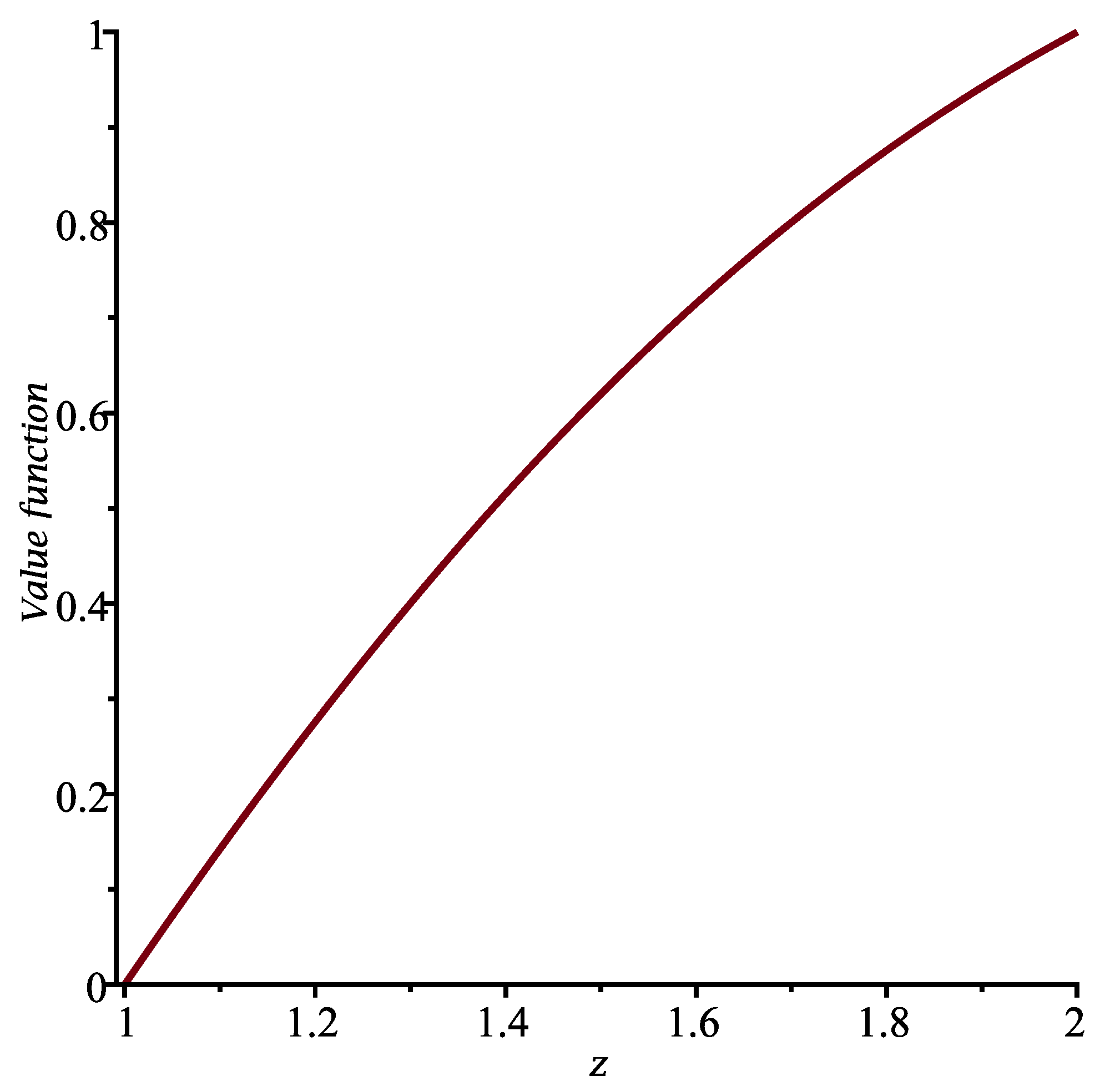
We present the function $H\left(z\right)$ in Figure 4. Furthermore, the optimal control is

$$u^{*}(x,y)=-x{F}_y(x,y)=-x^2{H}^{\prime }\left(xy\right)={\displaystyle \frac{2x^2\left({\mathit{e}}^{-1}-1\right){\mathit{e}}^{-2xy}}{-{\mathit{e}}^{-2xy-1}+{\mathit{e}}^{-3}+{\mathit{e}}^{-2xy}-{\mathit{e}}^{-4}}}.$$

(76)

See Figure 5 and Figure 6.

Case 2.

Suppose that $\rho (x,y)={\rho }_0/y$, where ${\rho }_0>0$. Under the same assumptions as in Case 1, the ODE satisfied by the function $\mathbf{\Psi }\left(z\right)$ is now

$$({\rho }_0-kz+m_{0}z){\mathbf{\Psi }}^{\prime }\left(z\right)+{\displaystyle \frac{1}{2}}{v}_0{z}^2{\mathbf{\Psi }}^{″}\left(z\right)=0.$$

(77)

The particular solution that satisfies the boundary conditions $\mathbf{\Psi }\left(k_i\right)=e^{-\gamma K_i}:={\kappa }_i$, for $i=1,2$, is

$$\mathbf{\Psi }\left(z\right)={\kappa }_1+{\displaystyle \frac{{\displaystyle ({\kappa }_2-{\kappa }_1){\int }_{{\mathit{k}}_{\mathit{1}}}^z{\mathit{e}}^{\frac{2{\rho }_0}{v_0\mathit{w}}}{\mathit{w}}^{\frac{2(k-m_0)}{v_0}}\mathrm{d}\mathit{w}}}{{\displaystyle {\int }_{{\mathit{k}}_{\mathit{1}}}^{{\mathit{k}}_{\mathit{2}}}{\mathrm{e}}^{\frac{2{\rho }_0}{v_0\mathit{w}}}{\mathit{w}}^{\frac{2(k-m_0)}{v_0}}\mathrm{d}\mathit{w}}}}.$$

(78)

The function $H\left(z\right)$ is displayed in Figure 7 when the constants are the same as in Case 1.

The optimal control is (see Equation (38))

$$u^{*}(x,y)=-x^2{H}^{\prime }\left(xy\right)\approx -{\displaystyle \frac{0.1517x^2{\mathit{e}}^{\frac{2}{xy}}}{{\displaystyle 1-0.1517{\int }_1^{xy}{\mathit{e}}^{2/w}\mathrm{d}\mathit{w}}}}.$$

(79)

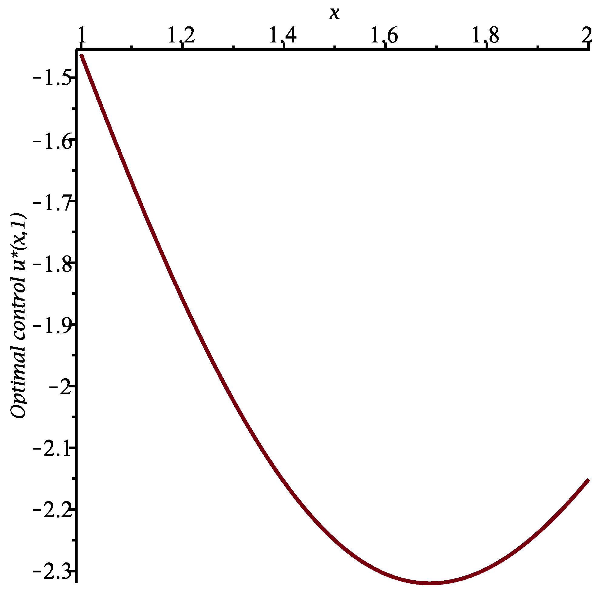
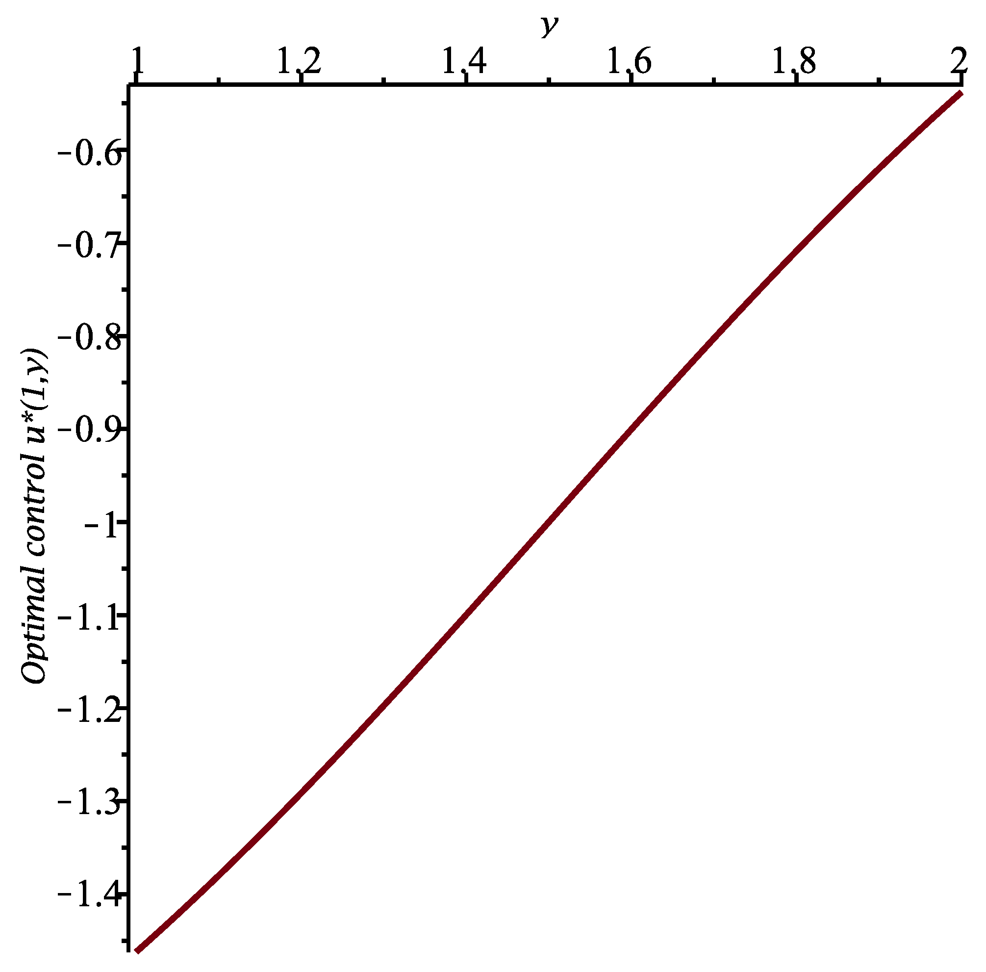
As in Case 1, the functions $u^{*}(x,1)$ and $u^{*}(1,x)$ are shown in Figure 8 and Figure 9, respectively.

5. Conclusions

In this paper, a queuing model in which customers arrive (approximately) according to a degenerate two-dimensional diffusion process was studied. The model is such that, in the case of the absence of service, the number of customers in the system is strictly increasing. Other authors have used diffusion processes as an approximation for the arrival of customers, but in only one dimension, for example a reflected Brownian motion.

Like any model, the one that we propose is based on simplifying assumptions. We believe it could be used successfully in certain applications, while traditional models might yield better results in others. The aim was to propose an alternative model that could prove useful in a variety of situations.

We wrote that the arrival process is approximated by a diffusion process. It should be emphasized that assuming that arrivals constitute a Poisson process, as in the case of the classic $M/M/s$ model, is also only an approximation of reality. Using an exponential distribution for the time between successive customer arrivals in the system is a simplifying assumption. In some applications, approximating arrivals using a Poisson process may be more realistic than using a diffusion process, while in other applications, the opposite is true.

In a special case, we were able to derive the distribution of the number $X\left(t\right)$ of customers in the system at time t. It would be interesting to obtain this distribution in other cases, or at least calculate the expected value of $X\left(t\right)$, as we did when $\left\{Y\right(t),t\ge 0\}$ is a geometric Brownian motion.

In Section 3, a stochastic control problem of the homing type was formulated for the queuing model. This is the first time that a homing problem has been studied for a queuing model such as the one proposed in the paper. We gave the non-linear partial differential equation satisfied by the value function, and we saw that it is sometimes possible to linearize this equation. Finally, several problems were solved explicitly and exactly by making use of the method of similarity solutions. When this method does not apply, we could use numerical techniques to find the value function and hence the optimal control for any particular problem.

References

1. Erlang, A.K. The theory of probabilities and telephone conversations. Nyt Tidss. Math. B 1909, 20, 33–39. [Google Scholar]
2. Erlang, A.K. Solution of some problems in the theory of probabilities of significance in automatic telephone exchanges. Elektroteknikeren 1917, 13, 5–13. [Google Scholar]
3. Khinchin, A.Y. Mathematical theory of a stationary queue. Mat. Sb. 1932, 39, 73–84. [Google Scholar]
4. Kendall, D.G. Some problems in the theory of queues. J. R. Stat. Soc. Ser. B Methodol. 1951, 13, 151–173. [Google Scholar] [CrossRef]
5. Jackson, J.R. Networks of waiting lines. Oper. Res. 1957, 5, 518–521. [Google Scholar] [CrossRef]
6. Cox, D.R.; Smith, W.L. Queues; Methuen: London, UK, 1961. [Google Scholar]
7. Kleinrock, L. Queueing Systems, Volume I: Theory; Wiley: New York, NY, USA, 1975. [Google Scholar]
8. Lee, H.W.; Yoon, S.H.; Lee, S.S. A continuous approximation for batch arrival queues with threshold. Computers Ops. Res. 1996, 23, 299–308. [Google Scholar] [CrossRef]
9. Lee, C.; Weerasinghe, A. Convergence of a queueing system in heavy traffic with general patience-time distributions. Stoch. Process. Their Appl. 2011, 121, 2507–2552. [Google Scholar] [CrossRef]
10. Lefebvre, M. A queuing model with arrivals according to a two-dimensional diffusion process. In Proceedings of the 5th Workshop on Intelligent Information Systems (WIIS2025), Chişinǎu, Republic of Moldova, 16–18 October 2025; pp. 206–213. [Google Scholar]
11. Rishel, R. Controlled wear process: Modeling optimal control. IEEE Trans. Autom. Control 1991, 36, 1100–1102. [Google Scholar] [CrossRef]
12. Harrison, J.M.; Reiman, M.I. Reflected Brownian motion in an orthant. Ann. Probab. 1981, 9, 303–308. [Google Scholar] [CrossRef]
13. Reiman, M.I. Open queueing networks in heavy traffic. Math. Oper. Res. 1984, 9, 441–458. [Google Scholar] [CrossRef]
14. Lefebvre, M. Applied Stochastic Processes; Springer: New York, NY, USA, 2007. [Google Scholar]
15. Whittle, P. Optimization over Time; Wiley: Chichester, UK, 1982; Volume I. [Google Scholar]
16. Lefebvre, M. Minimizing or maximizing the first-passage time to a time-dependent boundary. Optimization 2022, 71, 387–401. [Google Scholar] [CrossRef]
17. Makasu, C. Bounds for a risk-sensitive homing problem. Automatica 2024, 163, 111575. [Google Scholar] [CrossRef]
18. Laxmi, P.V.; Jyothsna, K. Optimization of service rate in a discrete-time impatient customer queue using particle swarm optimization. In Distributed Computing and Internet Technology, Proceedings of the International Conference on Distributed Computing and Internet Technology, Bhubaneswar, India, 15–18 January 2016; Springer International Publishing: Cham, Switzerland, 2016; pp. 38–42. [Google Scholar] [CrossRef]
19. Tian, R.; Su, S.; Zhang, Z.G. Equilibrium and social optimality in queues with service rate and customers’ joining decisions. Qual. Technol. Quant. Manag. 2024, 21, 1–34. [Google Scholar] [CrossRef]
20. Chen, G.; Liu, Z.; Xia, L. Event-based optimization of service rate control in retrial queues. J. Oper. Res. Soc. 2023, 74, 979–991. [Google Scholar] [CrossRef]
21. Dudin, A.; Dudin, S.; Dudina, O. Analysis of a queueing system with mixed service discipline. Methodol. Comput. Appl. Prob. 2023, 25, 19. [Google Scholar] [CrossRef]
22. Lakkumikanthan, I.; Balasubramanian, S. Optimal control of service rates of discrete-time (s,S) queueing—Inventory systems with finite buffer. In Proceedings of the 5th International Conference on Problems of Cybernetics and Informatics, Baku, Azerbaijan, 28–30 August 2023; pp. 1–4. [Google Scholar] [CrossRef]
23. Su, Y.; Li, J. Optimality of admission control in an M/M/1/N queue with varying services. Stoch. Model. 2021, 37, 317–334. [Google Scholar] [CrossRef]
24. Büke, B.; Qin, W. Many-server queues with random service rates in the Halfin-Whitt regime: A measure-valued process approach. arXiv 2019. [Google Scholar] [CrossRef]
25. Wu, C.-H.; Yang, D.-Y.; Yong, C.-R. Performance evaluation and bi-objective optimization for F-policy queue with alternating service rates. J. Ind. Manag. Optim. 2023, 19, 3819–3839. [Google Scholar] [CrossRef]
26. Lefebvre, M.; Yaghoubi, R. Optimal service time distribution for an M/G/1 waiting queue. Axioms 2024, 13, 594. [Google Scholar] [CrossRef]
Figure 1. Value function F ( x , y ) = H ( z = y / x ) (solid line) for 1 z 2 in Problem 1, when c = b 0 = q 0 = v 0 = 1 , k 1 = 1 , k 2 = 2 , K 1 = 0 and K 2 = 1 . The dotted line represents the expected cost H 0 ( z ) defined in Equation (61) if one uses no control.
Axioms 14 00868 g001
Figure 2. Optimal control u * ( x , 1 ) for 1 x 2 in Problem 1, when c = b 0 = q 0 = v 0 = 1 , k 1 = 1 , k 2 = 2 , K 1 = 0 and K 2 = 1 .
Axioms 14 00868 g002
Figure 3. Optimal control u * ( 1 , y ) for 1 y 2 in Problem 1, when c = b 0 = q 0 = v 0 = 1 , k 1 = 1 , k 2 = 2 , K 1 = 0 and K 2 = 1 .
Axioms 14 00868 g003
Figure 4. Value function F ( x , y ) = H ( z = x y ) for 1 z 2 in Problem 2, Case 1, when ρ 0 = k = b 0 = q 0 = m 0 = v 0 = 1 , k 1 = 1 , k 2 = 2 , K 1 = 0 and K 2 = 1 .
Axioms 14 00868 g004
Figure 5. Optimal control u * ( x , 1 ) for 1 x 2 in Problem 2, Case 1, when ρ 0 = k = b 0 = q 0 = m 0 = v 0 = 1 , k 1 = 1 , k 2 = 2 , K 1 = 0 and K 2 = 1 .
Axioms 14 00868 g005
Figure 6. Optimal control u * ( 1 , y ) for 1 y 2 in Problem 2, Case 1, when ρ 0 = k = b 0 = q 0 = m 0 = v 0 = 1 , k 1 = 1 , k 2 = 2 , K 1 = 0 and K 2 = 1 .
Axioms 14 00868 g006
Figure 7. Value function F ( x , y ) = H ( z = x y ) for 1 z 2 in Problem 2, Case 2, when ρ 0 = k = b 0 = q 0 = m 0 = v 0 = 1 , k 1 = 1 , k 2 = 2 , K 1 = 0 and K 2 = 1 .
Axioms 14 00868 g007
Figure 8. Optimal control u * ( x , 1 ) for 1 x 2 in Problem 2, Case 2, when ρ 0 = k = b 0 = q 0 = m 0 = v 0 = 1 , k 1 = 1 , k 2 = 2 , K 1 = 0 and K 2 = 1 .
Axioms 14 00868 g008
Figure 9. Optimal control u * ( 1 , y ) for 1 y 2 in Problem 2, Case 2, when ρ 0 = k = b 0 = q 0 = m 0 = v 0 = 1 , k 1 = 1 , k 2 = 2 , K 1 = 0 and K 2 = 1 .
Axioms 14 00868 g009
Disclaimer/Publisher’s Note: The statements, opinions and data contained in all publications are solely those of the individual author(s) and contributor(s) and not of MDPI and/or the editor(s). MDPI and/or the editor(s) disclaim responsibility for any injury to people or property resulting from any ideas, methods, instructions or products referred to in the content.