Article

An Infeasibility Condition for Rank Reversal in the Analytic Hierarchy Process

1
Xianda College of Economics and Humanities, Shanghai International Studies University, Shanghai 200083, China
2
School of Statistics and Data Science, Shanghai University of Finance and Economics, Shanghai 200433, China
*
Author to whom correspondence should be addressed.
Axioms 2025, 14(12), 860; https://doi.org/10.3390/axioms14120860
Submission received: 15 October 2025 / Revised: 17 November 2025 / Accepted: 20 November 2025 / Published: 24 November 2025
(This article belongs to the Section Mathematical Analysis)

Abstract

The analytic hierarchy process (AHP) is one of the most widely applied tools in Multi-Criteria Decision Making (MCDM), yet it is often criticized for rank reversal when a new option is introduced. We present an infeasibility condition under which rank reversal is theoretically impossible. The condition serves as a sufficient criterion for rank stability, clarifying when the overall ranking remains invariant despite the addition of new alternatives. If the condition is not satisfied, rank reversal may occur, explaining why it appears in some applications but not in others.
MSC:
90B50; 91B06; 90C29

1. Introduction

Management science is an interdisciplinary field with a wide spectrum of real-world applications [1,2,3,4], including decision analysis, industrial engineering, and so on. Multiple Criteria Decision Making (MCDM) is a sub-discipline dealing with conflicting criteria [5,6,7]. The analytic hierarchy process (AHP), developed by Saaty [8] (also see Saaty [9] and Saaty [10]), has been widely investigated by scientists over the last four decades as one MCDM tool [11,12]. Many applications and empirical studies indicate that the AHP seems to be an appealing MCDM tool. However, practitioners are aware that the AHP has its controversial issues in real-world applications, e.g., Jiang et al. [13], Triantaphyllou and Yanase [14], Starczewski [15].
In this study, we focus on one of the most discussed controversial issues in the AHP, the rank reversal problem. A typical AHP application involves multiple options and multiple criteria. All the options are judged by each criterion so that each criterion yields a priority vector. An aggregate priority vector is obtained by a weighted sum of all priority vectors using weights. The options can be ranked by the aggregate priority vector. When an option is added to the original set of options, all priority vectors vary so that the aggregate priority vector also varies. The rank reversal problem refers to the ranks of two options in the original set are possibly reversed in the augmented option set [16]. From a practitioner’s point of view, adding a new option is similar to the insertion in a queue, and the order of the original queue had better be left untouched. Consequently, the rank reversal problem is annoying and even causes one to doubt the whole AHP framework.
While Belton and Gear [16] provide an instance of the rank reversal problem, they also suggest a new form of normalization in which the priorities of the options should be re-scaled by the maximum value instead of their sum. As a matter of fact, Belton and Gear [16] propose a variant of AHP, i.e., the BG-revised AHP. There are other variants of AHP which are assumed to alleviate or eliminate the rank reversal problem [11]. Schoner and Wedley [17] propose a variant called the Reference AHP. Schoner et al. [18] introduce a variant called the linking pin AHP. The multiplicative AHP has been investigated by Lootsma [19], Barzilai and Golany [20], Barzilai and Lootsma [21], Lootsma and Barzilai [22], Stam [23], Triantaphyllou [24], and Stam and Silva [25]. However, whether these variants can achieve their claims is in doubt. For instance, Saaty and Vargas [26] provide a counter-example to show that the BG-revised AHP from Belton and Gear [16] fails to fix the rank reversal problem. Belton and Gear [27] make a comment to explain that there is a misinterpretation of their suggested procedure and the rank reversal problem is solved since the weights of the criteria are also properly amended during the new normalization. Barzilai and Golany [20] suggest that the BG-revised AHP does not solve the rank reversal problem. Peng et al. [28] claim that the BG-revised AHP is shown to be incorrect. Similar controversies occur for other AHP variants. Vargas [29] points out that the multiplicative AHP has its own issues in terms of rank-preservation. Tu and Wu [30] revisit the structural origins of rank reversal in the AHP and identify three major causes—preference intransitivity, prioritization procedure, and aggregation rule. They propose an optimization-based prioritization framework, the NRV-LSE model, to enhance rank stability.
There are many well-known MCDM tools other than the AHP [11,31], including the Analytic Network Process (ANP) presented in Saaty [32], a much more complicated extension of the AHP; the Technique for Order of Preference by Similarity to Ideal Solution (TOPSIS) presented in Hwang and Yoon [5]; Elimination and Choice Translating Reality (ELECTRE), outlined in Roy [33]; and the Preference Ranking Organization Method for Enrichment Evaluations (PROMETHEE) shown in Brans and Vincke [34] and Mareschal and Brans [35]. The rank reversal problem also occurs when these MCDM tools are used. For instance, Jiang et al. [13] conducted large-scale simulations across multiple MCDM methods, showing that rank reversal is not an accidental artifact but a structural and probabilistic property of decision models. These recent findings highlight that rank instability persists even under improved consistency or normalization schemes, reinforcing the need for a theoretical framework—such as the infeasibility condition proposed in this paper—to explicitly delineate the boundaries of rank stability in the AHP.
Instead of modifying the AHP procedure itself, we seek to identify a mathematical condition under which it is impossible for rank reversal to occur. As summarized by Maleki and Zahir [11], four types of rank reversal may arise when the following changes occur:
(i)
A new option is added;
(ii)
An existing option is deleted;
(iii)
A new criterion is added;
(iv)
An existing criterion is deleted.
Among these scenarios, the addition of a new option is the most common and practically significant one, and thus becomes the focus of our investigation. We will propose a formal framework and derive an infeasibility condition, ensuring that rank reversal can never occur. If this condition fails, then rank reversal becomes theoretically possible—explaining why it may or may not be observed in real-world applications.
Our investigation is organized as follows. Section 2 introduces the problem of rank reversal using the example in Belton and Gear [16], points out multiple steps used by the AHP to obtain an aggregate priority vector, and states our focus on the last step. Section 3 formalizes the process of addition of a new option. Section 4 formalizes the rank reversal problem and presents the infeasibility condition. For the purpose of illustration, Section 5 presents the Belton–Gear example and four synthetic examples. Section 6 summarizes our analyses and suggests some prospective possibilities of investigation.
We expect that our study can provide a theoretical boundary that clarifies when rank reversal is theoretically impossible, offering a new perspective on rank stability in the AHP beyond empirical or optimization-based approaches.

2. The Problem of Rank Reversal

2.1. The Belton–Gear Example

Belton and Gear [16] present an example in which the decision-maker considers three criteria with identical importance. Initially, the options are introduced, and there are three pairwise comparison matrices, as follows:
1 1 / 9 1 9 1 9 1 1 / 9 1 , 1 9 9 1 / 9 1 1 1 / 9 1 1 , 1 8 / 9 8 9 / 8 1 9 1 / 8 1 / 9 1 .
When a new option is introduced, the updated versions are given by
1 1 / 9 1 1 / 9 9 1 9 1 1 1 / 9 1 1 / 9 9 1 9 1 , 1 9 9 9 1 / 9 1 1 1 1 / 9 1 1 1 1 / 9 1 1 1 , 1 8 / 9 8 8 / 9 9 / 8 1 9 1 1 / 8 1 / 9 1 1 / 9 9 / 8 1 9 1 .
Belton and Gear [16] obtain the aggregate priority vector from (1) for the first three options as follows:
1 594 ( 268 , 279 , 47 ) ,
and the one from (2) for the four options as follows:
1 405 ( 148 , 117 , 23 , 117 ) ,
albeit pure decimals rather than fractions are used in Belton and Gear [16]. It is clear that the ranks of the first two options in (3) are reversed in (4) as 268 < 279 , while 148 > 117 .
The pairwise comparison matrices in (1) and (2) are cardinally consistent in the sense that there exists a unique priority vector p = ( p 1 , p 2 , , p n ) , generating a pairwise comparison matrix ( a i j ) n × n with a i j = p i / p j , n 2 . Given this particular example, the problem of rank reversal does not come from cardinal inconsistency but arises from the priority vectors.
Barzilai and Golany [20] present an example in which those pairwise comparison matrices are not cardinally consistent. They find that the rank reversal problem persists. An algorithm applied to a cardinally inconsistent pairwise comparison matrix can yield a priority vector. The priority vector induces a cardinally consistent pairwise comparison matrix, which is understood as an approximation of the cardinally inconsistent one.
These mean that the rank reversal problem can be complicated. We should approach the problem under various sets of assumptions, instead of dreaming of accomplishing the whole task in one stroke.

2.2. Four Steps Arising from the Usual AHP

It can be easily observed that there are four steps leading to an aggregate priority vector using the usual AHP framework [12] (see Figure 1). When a new option is added, the previous four steps can be repeated to produce an augmented priority vector.
As a matter of fact, an observation of rank reversal is possibly related to each of these four steps. Firstly, the ranks are directly generated from an aggregate priority vector and an augmented priority vector. Secondly, the other three steps have direct or indirect impacts on the two aggregate priority vectors, and consequently, have indirect impacts on the rank reversal problem.
Our present investigation will focus on Step 4 in Figure 1. This does not mean the other three steps are negligible. Separate investigations are necessary to reveal those complicated indirect impacts arising from the other three steps.

3. The Option Set and Its Augmentation

We will formalize the addition of an option. Initially, we have an option set Q n = { x 1 , x 2 , , x n } of size n and a criterion set C = { c 1 , c 2 , , c m } of size m. The criterion set C produces a priority vector λ = ( λ 1 , λ 2 , , λ m ) with = 1 m λ = 1 and λ ( 0 , 1 ) , 1 m . The priority vector of Q n , given criterion c , is w = ( w 1 , , w 2 , , , w n , ) , 1 m . The aggregate priority vector of Q n is
w ¯ n = ( w ¯ 1 , w ¯ 2 , , w ¯ n ) = = 1 m λ w .
Suppose that a new option x n + 1 is added into Q n and the augmented option set is denoted by Q n + 1 . The priority vector of Q n + 1 given criterion c is
u = ( u 1 , , u 2 , , , u n , , u n + 1 , ) .
The aggregate priority vector of Q n + 1 is
u ¯ n + 1 = ( u ¯ 1 , u ¯ 2 , , u ¯ n , u ¯ n + 1 ) = = 1 m λ u .
As j = 1 n + 1 u j , = 1 , it holds that j = 1 n u j , = 1 u n + 1 , and
u j , = γ · w j , , 1 j n , 1 m , u n + 1 , = γ · { ( 1 γ ) / γ } ,
where
γ = 1 u n + 1 , .
The aggregate priority vector u ¯ n + 1 can be rewritten as
u ¯ n + 1 = = 1 m λ γ w 1 , , w 2 , , , w n , , 1 γ γ = = 1 m λ γ w , 1 γ γ .
Since we only consider the ranks of the first n options from the aggregate priority vector of the augmented option set Q n + 1 , we will focus on
u ¯ n = = 1 m λ γ w ,
which is the sub-vector of u ¯ n + 1 in (9), consisting of its first n entries.
Let ν = = 1 m λ γ . As γ ( 0 , 1 ) , 0 < ν < = 1 m λ = 1 . Define
a = λ γ / ν , = 1 , 2 , , m ,
It holds that = 1 m a = 1 . Define a scaled version of u ¯ n in (10) as follows:
z ¯ n = = 1 m a · w = u ¯ n ν .

4. The Infeasibility Condition

Next, we will formalize the rank reversal problem and derive the infeasibility condition for its occurrence. We will study the problem of rank reversal via (5), (10), and (12).
The rank reversal problem can happen between any of those n 2 pairs of options. We consider the option pair ( j , k ) and 1 j < k n , and re-define
y 1 , = w j , , y 2 , = w k , , y = ( y 1 , , y 2 , ) .
Let T denote a triangle, as follows:
T = { y R 2 : y 1 + y 2 < 1 , 0 < y 1 < 1 , 0 < y 2 < 1 } ,
which excludes its three sides and only consists of interior points. Because 0 < y 1 , < 1 , 0 < y 2 , < 1 , and y 1 , + y 2 , < 1 , the triangle T includes the set { y } = 1 m .
The internal angle bisector of the triangle T is
B = { y R 2 : y 1 + y 2 < 1 , 0 < y 1 < 1 , 0 < y 2 < 1 , y 1 = y 2 } .
Let B ¯ and B ̲ represent the triangles above and below B, respectively, where
B ¯ = { y R 2 : y 1 + y 2 < 1 , 0 < y 1 < 1 , 0 < y 2 < 1 , y 1 < y 2 } ,
B ̲ = { y R 2 : y 1 + y 2 < 1 , 0 < y 1 < 1 , 0 < y 2 < 1 , y 1 > y 2 } .
Given y = ( y 1 , y 2 ) R 2 , let rank ( y ) denote the vector of ranks of y 1 and y 2 . When there are ties, average ranks are used. Note that, given y T ,
rank ( y ) = ( 2 , 1 ) y B ¯ ( 1 , 2 ) y B ̲ ( 1.5 , 1.5 ) y B .
There are three vectors as sub-vectors: w ¯ n in (5), u ¯ n in (10), and z ¯ n in (12), respectively.
ψ = = 1 m λ · y ,
ϕ = = 1 m λ γ · y ,
σ = = 1 m a · y .
As σ = ϕ / ν , it is clear that rank ( σ ) = rank ( ϕ ) , which means that the rank reversal problem can be studied via (18) and (20).
Both σ and ψ are in H, where
H = conv ( y 1 , y 2 , , y m ) ,
and conv ( · ) denotes the convex hull of a subset of R 2 . The rank reversal occurs if σ B ¯ and ψ B ̲ , or ψ B ¯ and σ B ̲ , under the condition that
B ¯ H & B ̲ H .
There are three kinds of exclusive configurations of the m points, y 1 , y 2 , , y m , within the triangle T in (14). In the first kind of configuration, all points are in the triangle B ¯ in (16), with one side B in (15), i.e.,
= 1 m I y 1 , y 2 , B B ¯ = 1 ,
where I ( · ) is the indicator function. In the second kind of configuration, all points are in the triangle B ̲ in (17), with one side B in (15), i.e.,
= 1 m I y 1 , y 2 , B B ̲ = 1 .
In the third kind of configuration, one can select one point in B ¯ in (16), select one point in B ̲ in (17), and leave all other points anywhere in T in (14), i.e.,
= 1 m I y 1 , y 2 , B B ¯ + = 1 m I y 1 , y 2 , B B ̲ = 0 ,
which is equivalent to the condition in (22).
Suppose that the two assumptions in (22) hold. Consider constructing an option that induces reversed ranks. If ψ B ¯ (or B ̲ ), then one can choose a 1 , a 2 , , a m , such that σ B ̲ H (or B ¯ H ). Next, we will seek { γ } = 1 m given a 1 , a 2 , , a m , λ 1 , λ 2 , , λ m . Let
τ = min { λ 1 / a 1 , λ 2 / a 2 , , λ m / a m } .
If τ > 1 , then λ i / a i > 1 or λ i > a i , 1 i m , and 1 = i = 1 m λ i > i = 1 m a i = 1 . Conclude that τ 1 . Choose any ν ( 0 , τ ) ( 0 , 1 ] and define
γ = ν a / λ , 1 m .
From (26) and (27), and the choice of ν , we conclude that
γ ( 0 , 1 ) , 1 m .
Because of (28), an added option can be defined via (7), (8), and (27). This means that one can construct an aggregate priority vector of the augmented option set Q n + 1 with rank reversals when it is feasible.
These findings can be summarized as the following theorem.
Theorem 1.
Let W = ( w 1 , w 2 , , w m ) . Given 1 j < k n , the rank reversal problem between the two options x j and x k is infeasible if, and only if, ρ j , k ( W ) = 1 , and the rank reversal problem among these n options is infeasible if, and only if, ρ ( W ) = 1 , where
ρ ( W ) = 1 j < k n ρ j , k ( W ) ,
ρ j , k ( W ) = = 1 m I w j , w k , B B ¯ + = 1 m I w j , w k , B B ̲ .

5. Illustration

5.1. The Belton–Gear Example Revisited

We revisit the classical example in Belton and Gear [16]. The original option set has three options ( n = 3 ) and the augmented one has four options. The criterion set has three criteria ( m = 3 ). The three criteria are assumed to be equally important, i.e., λ = 1 / 3 , = 1 , 2 and 3. The three priority vectors of the original option set and those of the augmented option set are given as follows:
w 1 = 1 11 1 9 1 , w 2 = 1 11 9 1 1 , w 3 = 1 18 8 9 1 ,
u 1 = 1 20 1 9 1 9 , u 2 = 1 12 9 1 1 1 , u 3 = 1 27 8 9 1 9 ,
Let W = ( w 1 , w 2 , w 3 ) . One can easily derive (31) from (1), (32) from (2), (3) from (31), and (4) from (32). It is also clear that
γ 1 = 1 9 / 20 = 11 / 20 , γ 2 = 1 1 / 12 = 11 / 12 , γ 3 = 1 9 / 27 = 18 / 27 , ν = ( 11 / 20 + 11 / 12 + 18 / 27 ) / 3 = 32 / 45 , a 1 = λ 1 γ 1 / ν = 33 / 128 , a 2 = λ 2 γ 2 / ν = 55 / 128 , a 3 = λ 3 γ 3 / ν = 40 / 128 , a 1 + a 2 + a 3 = 1 .
With ( 1 / 405 ) / ( 32 / 45 ) = 1 / 288 , to summarize, we write
w ¯ 3 = 1 594 268 279 47 , u ¯ 3 = 1 405 148 117 23 , z ¯ 3 = 1 288 148 117 23 .
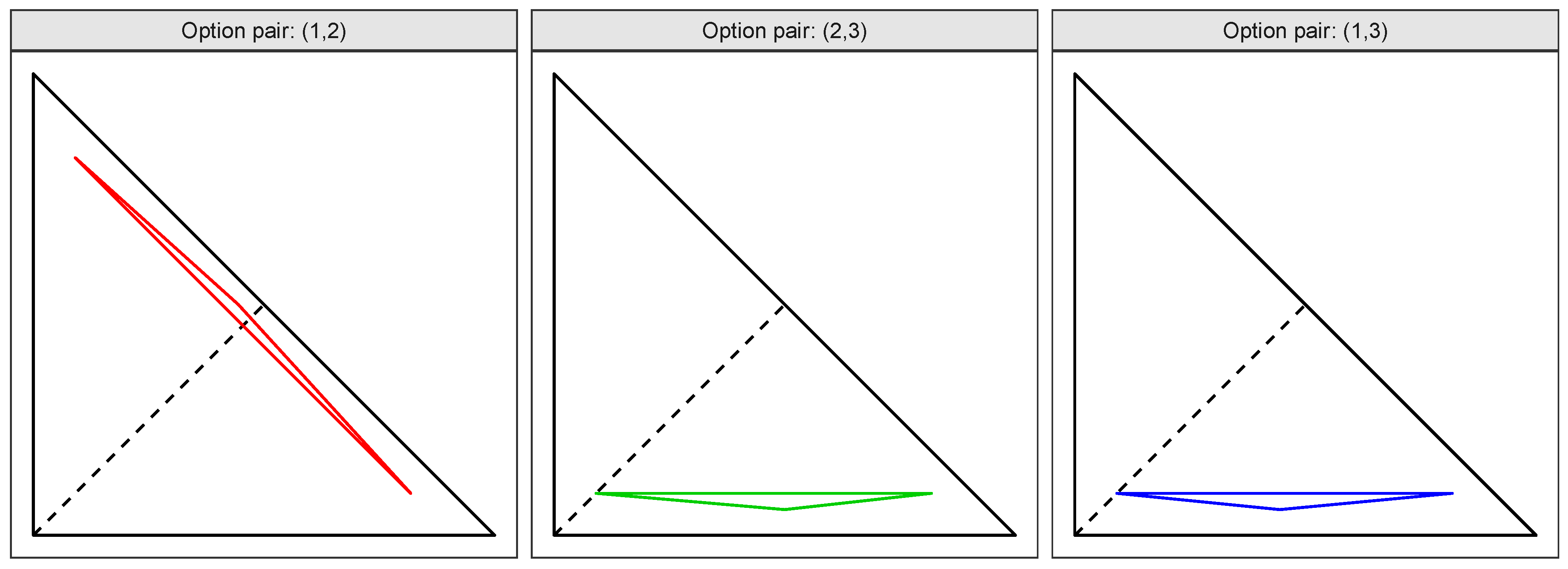
Firstly, consider the option pair ( 1 , 2 ) . The three projection points are as follows:
y 1 = 1 11 ( 1 , 9 ) , y 2 = 1 11 ( 9 , 1 ) , y 3 = 1 18 ( 8 , 9 ) .
Note that y 1 B ¯ , y 3 B ¯ , and y 2 B ̲ . These mean that their convex hull has a nonempty intersection with both B ¯ and B ̲ , i.e., ρ 1 , 2 ( W ) = 0 . Figure 2 presents the convex hull of y 1 , y 2 , y 3 , a triangle with vertices y 1 , y 2 , y 3 , one part in B ¯ , one part in B ̲ , and one line segment in B. Because ψ B ¯ and σ B ̲ , the ranks of options 1 and 2 are reversed, where
ψ = 1 594 ( 268 , 279 ) , ϕ = 1 405 ( 148 , 117 ) , σ = 1 288 ( 148 , 117 ) .
Secondly, consider the option pair ( 2 , 3 ) . The three projection points are as follows:
y 1 = 1 11 ( 9 , 1 ) , y 2 = 1 11 ( 1 , 1 ) , y 3 = 1 18 ( 9 , 1 ) .
As y 2 B , y 1 B ̲ , and y 3 B ̲ , ρ 2 , 3 ( W ) = 1 . Figure 2 presents the convex hull of y 1 , y 2 , y 3 , a triangle residing in B ̲ with a single vertex y 2 B . The ranks of options 2 and 3 can not be reversed. Write
ψ = 1 594 ( 279 , 47 ) , ϕ = 1 405 ( 117 , 23 ) , σ = 1 288 ( 117 , 23 ) .
Thirdly, consider the option pair ( 1 , 3 ) . The three projection points are as follows:
y 1 = 1 11 ( 1 , 1 ) , y 2 = 1 11 ( 9 , 1 ) , y 3 = 1 18 ( 8 , 1 ) .
As y 1 B , y 2 B ̲ , and y 3 B ̲ , ρ 1 , 3 ( W ) = 1 . Figure 2 presents the convex hull of y 1 , y 2 , y 3 , a triangle residing in B ̲ with a single vertex y 1 B . The ranks of options 1 and 3 can not be reversed. Write
ψ = 1 594 ( 268 , 47 ) , ϕ = 1 405 ( 148 , 23 ) , σ = 1 288 ( 148 , 23 ) .
Finally, the infeasibility condition fails, which can be easily seen from
ρ ( W ) = ρ 1 , 2 ( W ) × ρ 2 , 3 ( W ) × ρ 1 , 3 ( W ) = 0 × 1 × 1 = 0 ,
as there is an option pair ( 1 , 2 ) , whose ranks can be reversed. The added option is a realization of rank reversal.

5.2. Four Synthetic Examples

We will present four examples, each being represented by W = ( w 1 , w 2 , w 3 ) , with each column standing for one priority vector of three options. There are three option pairs, being indexed by ( 1 , 2 ) , ( 2 , 3 ) , and ( 1 , 3 ) , respectively.
Example A has
W A = 1 12 1 1 9 2 9 1 9 2 2 .
Given the option pair ( j , k ) = ( 1 , 2 ) , ( 2 , 3 ) , ( 1 , 3 ) from W A , respectively, we obtain
A - ( 1 , 2 ) : y 1 = 1 12 ( 1 , 2 ) B ¯ , y 2 = 1 12 ( 1 , 9 ) B ¯ , y 3 = 1 12 ( 9 , 1 ) B ̲ ,
A - ( 2 , 3 ) : y 1 = 1 12 ( 2 , 9 ) B ¯ , y 2 = 1 12 ( 9 , 2 ) B ̲ , y 3 = 1 12 ( 1 , 2 ) B ¯ ,
A - ( 1 , 3 ) : y 1 = 1 12 ( 1 , 9 ) B ¯ , y 2 = 1 12 ( 1 , 2 ) B ¯ , y 3 = 1 12 ( 9 , 2 ) B ̲ .
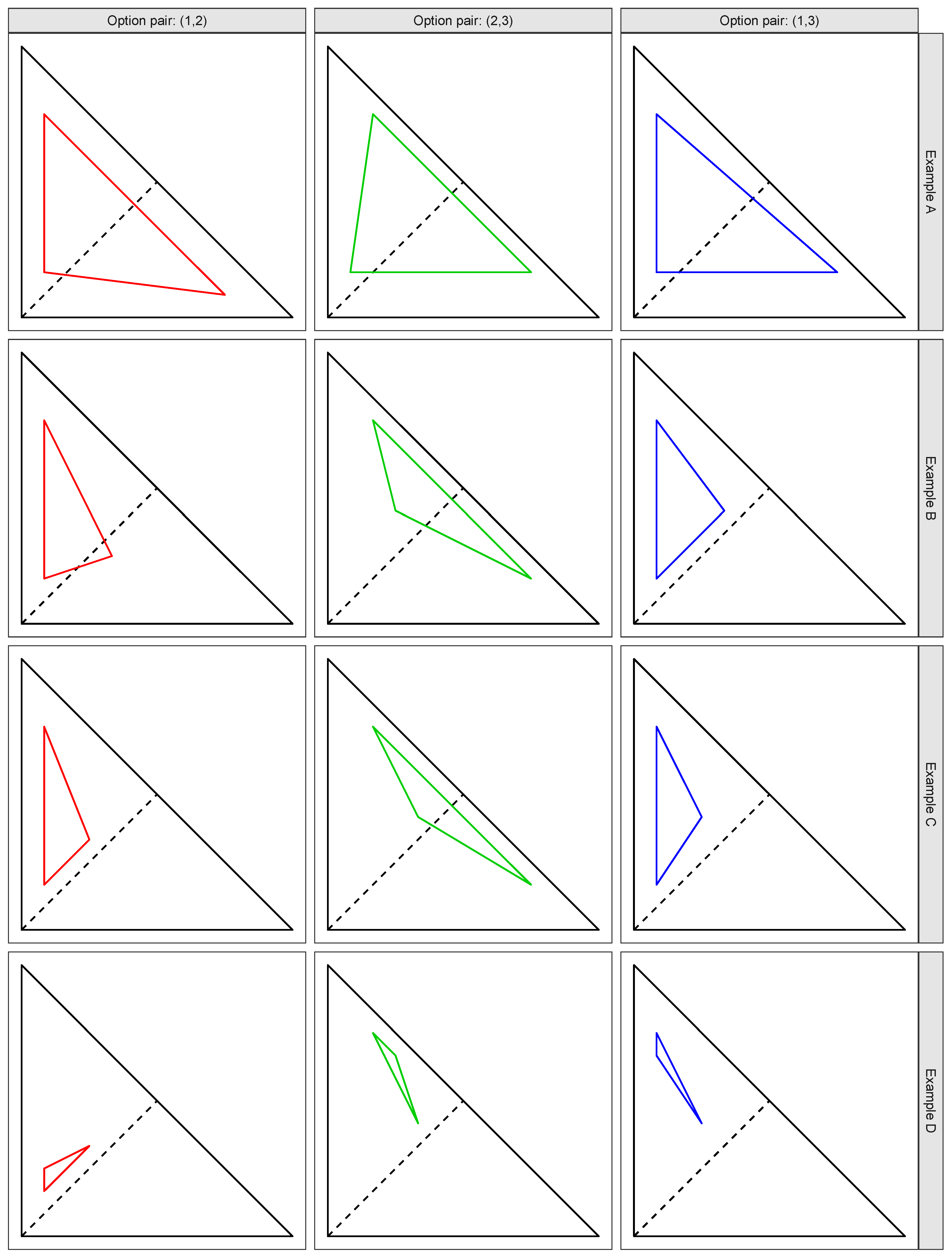
In (38), both y 1 and y 2 are in B ¯ , while y 3 is in B ̲ , and the convex hull of { y 1 , y 2 , y 3 } has a nonempty intersection with B ¯ and a nonempty intersection with B ̲ . Similar conclusions can be made from (39) and from (40). We summarize these conclusions in the following:
A - ( 1 , 2 ) : conv ( y 1 , y 2 , y 3 ) B ¯ , conv ( y 1 , y 2 , y 3 ) B ̲ ,
A - ( 2 , 3 ) : conv ( y 1 , y 2 , y 3 ) B ¯ , conv ( y 1 , y 2 , y 3 ) B ̲ ,
A - ( 1 , 3 ) : conv ( y 1 , y 2 , y 3 ) B ¯ , conv ( y 1 , y 2 , y 3 ) B ̲ .
The infeasibility condition does not hold for Example A due to (41)–(43), i.e.,
ρ ( W A ) = ρ 1 , 2 ( W A ) × ρ 2 , 3 ( W A ) × ρ 1 , 3 ( W A ) = 0 × 0 × 0 = 0 .
Example B has
W B = 1 12 1 1 4 2 9 3 9 2 5 .
We observe that
B - ( 1 , 2 ) : y 1 = 1 12 ( 1 , 2 ) B ¯ , y 2 = 1 12 ( 1 , 9 ) B ¯ , y 3 = 1 12 ( 4 , 3 ) B ̲ ,
B - ( 2 , 3 ) : y 1 = 1 12 ( 2 , 9 ) B ¯ , y 2 = 1 12 ( 9 , 2 ) B ̲ , y 3 = 1 12 ( 3 , 5 ) B ¯ ,
B - ( 1 , 3 ) : y 1 = 1 12 ( 1 , 9 ) B ¯ , y 2 = 1 12 ( 1 , 2 ) B ¯ , y 3 = 1 12 ( 4 , 5 ) B ¯ ,
and consequently,
B - ( 1 , 2 ) : conv ( y 1 , y 2 , y 3 ) B ¯ , conv ( y 1 , y 2 , y 3 ) B ̲ ,
B - ( 2 , 3 ) : conv ( y 1 , y 2 , y 3 ) B ¯ , conv ( y 1 , y 2 , y 3 ) B ̲ ,
B - ( 1 , 3 ) : conv ( y 1 , y 2 , y 3 ) B ¯ .
The infeasibility condition does not hold for Example B due to (48) and (49), i.e.,
ρ ( W B ) = ρ 1 , 2 ( W B ) × ρ 2 , 3 ( W B ) × ρ 1 , 3 ( W B ) = 0 × 0 × 1 = 0 .
Example C has
W C = 1 12 1 1 3 2 9 4 9 2 5 .
We observe that
C - ( 1 , 2 ) : y 1 = 1 12 ( 1 , 2 ) B ¯ , y 2 = 1 12 ( 1 , 9 ) B ¯ , y 3 = 1 12 ( 3 , 4 ) B ¯ ,
C - ( 2 , 3 ) : y 1 = 1 12 ( 2 , 9 ) B ¯ , y 2 = 1 12 ( 9 , 2 ) B ̲ , y 3 = 1 12 ( 4 , 5 ) B ¯ ,
C - ( 1 , 3 ) : y 1 = 1 12 ( 1 , 9 ) B ¯ , y 2 = 1 12 ( 1 , 2 ) B ¯ , y 3 = 1 12 ( 3 , 5 ) B ¯ ,
and consequently,
C - ( 1 , 2 ) : conv ( y 1 , y 2 , y 3 ) B ¯ ,
C - ( 2 , 3 ) : conv ( y 1 , y 2 , y 3 ) B ¯ , conv ( y 1 , y 2 , y 3 ) B ̲ ,
C - ( 1 , 3 ) : conv ( y 1 , y 2 , y 3 ) B ¯ .
The infeasibility condition does not hold for Example C due to (56), i.e.,
ρ ( W C ) = ρ 1 , 2 ( W C ) × ρ 2 , 3 ( W C ) × ρ 1 , 3 ( W C ) = 1 × 0 × 1 = 0 .
Example D has
W D = 1 12 1 1 3 2 3 4 9 8 5 .
We observe that
D - ( 1 , 2 ) : y 1 = 1 12 ( 1 , 2 ) B ¯ , y 2 = 1 12 ( 1 , 3 ) B ¯ , y 3 = 1 12 ( 3 , 4 ) B ¯ ,
D - ( 2 , 3 ) : y 1 = 1 12 ( 2 , 9 ) B ¯ , y 2 = 1 12 ( 3 , 8 ) B ¯ , y 3 = 1 12 ( 4 , 5 ) B ¯ ,
D - ( 1 , 3 ) : y 1 = 1 12 ( 1 , 9 ) B ¯ , y 2 = 1 12 ( 1 , 8 ) B ¯ , y 3 = 1 12 ( 4 , 5 ) B ¯ ,
and consequently,
D - ( 1 , 2 ) : conv ( y 1 , y 2 , y 3 ) B ¯ ,
D - ( 2 , 3 ) : conv ( y 1 , y 2 , y 3 ) B ¯ ,
D - ( 1 , 3 ) : conv ( y 1 , y 2 , y 3 ) B ¯ .
The infeasibility condition does hold for Example D, i.e.,
ρ ( W D ) = ρ 1 , 2 ( W D ) × ρ 2 , 3 ( W D ) × ρ 1 , 3 ( W D ) = 1 × 1 × 1 = 1 .
Figure 3 presents the convex hulls in (41)–(43), (48)–(50), (55)–(57), and (62)–(64), arising from the four examples in (37), (44), (51), and (58).

6. Conclusions

This paper establishes a mathematical framework which can be used to analyze the infeasibility of rank reversal in the AHP. By formulating the aggregation and normalization procedures as convex combinations of criterion-wise priority vectors, we derive an explicit infeasibility condition that delineates when rank reversal will never occur. The condition provides a sufficient criterion for rank stability, showing that if all criterion-wise projections of any pair of alternatives lie on the same side of the bisector, the overall ranking remains unchanged, regardless of the addition of any new option.
Our framework can be used to assess the results in the literature on the rank reversal problem in which contradictory statements have been made over more than forty years of debates [11,16,28].
The proposed framework also complements recent studies by providing a geometric and verifiable boundary for rank stability. It offers a diagnostic tool for assessing the robustness of AHP results and can be possibly extended to other MCDM settings [13]. Future research may focus on extending the infeasibility condition to alternative scenarios, such as the addition or deletion of criteria [11].

Author Contributions

Conceptualization, J.Y. and C.M.; methodology and mathematical derivations, J.Y. and C.M.; validation and theoretical review, C.M.; visualization, J.Y.; writing—original draft preparation, J.Y.; writing—review and editing, C.M. All authors have read and agreed to the published version of the manuscript.

Funding

This research received no external funding.

Data Availability Statement

No new data were created in this study. Data sharing is not applicable to this article.

Acknowledgments

The authors used OpenAI’s ChatGPT (GPT-5) to assist with code annotation and proof-reading during manuscript preparation. The authors have reviewed and edited both the R codes and outputs, and take full responsibility for the content of this publication.

Conflicts of Interest

The authors declare no conflicts of interest.

Abbreviations

The following abbreviations are used in this manuscript:
AHPAnalytic Hierarchy Process
MCDMMulti-Criteria Decision Making

References

  1. Wolf, B.; Häring, A.-M.; Heß, J. Strategies towards evaluation beyond scientific impact: Pathways not only for agricultural research. Org. Farming 2015, 1, 3–18. [Google Scholar] [CrossRef]
  2. Chaoui, G.; Yaagoubi, R.; Mastere, M. Integrating geospatial technologies and multi-criteria decision analysis for sustainable and resilient urban planning. Chall. Sustain. 2025, 13, 122–134. [Google Scholar] [CrossRef]
  3. Fedorka, P.; Buchuk, R.; Klymenko, M.; Saibert, F.; Petrushyn, A. The use of adaptive artificial intelligence learning models in decision support systems for smart regions. J. Res. Innov. Technol. 2025, 4, 99–115. [Google Scholar]
  4. Terentieva, N.; Karpenko, V.; Yarova, N.; Shkvyria, N.; Pasko, M. Technological innovation in digital brand management: Leveraging artificial intelligence and immersive experiences. J. Res. Innov. Technol. 2025, 4, 201–223. [Google Scholar]
  5. Hwang, C.-L.; Yoon, K. Multiple Attribute Decision Making: Methods and Applications, a State-of-the-Art Survey; Springer: Berlin/Heidelberg, Germany, 1981. [Google Scholar]
  6. Krause, A.; Köppel, J. A multi-criteria approach for assessing the sustainability of small-scale cooking and sanitation technologies. Chall. Sustain. 2018, 6, 1–19. [Google Scholar] [CrossRef]
  7. Qiu, Y.; Bouraima, M.B.; Badi, I.; Stević, Ž.; Simic, V. A decision-making model for prioritizing low-carbon policies in climate change mitigation. Chall. Sustain. 2024, 12, 1–17. [Google Scholar] [CrossRef]
  8. Saaty, T.L. The Analytic Hierarchy Process; McGraw-Hill: New York, NY, USA, 1980. [Google Scholar]
  9. Saaty, T.L. A scaling method for priorities in hierarchical structures. J. Math. Psychol. 1977, 15, 234–281. [Google Scholar] [CrossRef]
  10. Saaty, T.L. How to make a decision: The analytic hierarchy process. Eur. J. Oper. Res. 1990, 48, 9–26. [Google Scholar] [CrossRef]
  11. Maleki, H.; Zahir, S. A comprehensive literature review of the rank reversal phenomenon in the analytic hierarchy process. J. Multi-Criteria Decis. Anal. 2013, 20, 141–155. [Google Scholar] [CrossRef]
  12. Brunelli, M. Introduction to the Analytic Hierarchy Process; Springer: Berlin/Heidelberg, Germany, 2015. [Google Scholar]
  13. Jiang, L.; Liao, H.; De Baets, B. A simulation study on the probabilities of rank reversal, tie making, and tie breaking for multiple criteria decision-making methods. Omega 2024, 125, 103033. [Google Scholar] [CrossRef]
  14. Triantaphyllou, E.; Yanase, J. The use of pairwise comparisons for decision making may lead to grossly inaccurate results. Comput. Ind. Eng. 2024, 198, 110653. [Google Scholar] [CrossRef]
  15. Starczewski, T. Rounding errors in pairwise comparisons matrices by Monte Carlo analysis. J. Appl. Math. Comput. Mech. 2025, 24, 71–85. [Google Scholar] [CrossRef]
  16. Belton, V.; Gear, T. On a short-coming of Saaty’s method of analytic hierarchies. Omega 1983, 11, 228–230. [Google Scholar] [CrossRef]
  17. Schoner, B.; Wedley, W.C. Ambiguous criteria weights in AHP: Consequences and solutions. Decis. Sci. 1989, 20, 462–475. [Google Scholar] [CrossRef]
  18. Schoner, B.; Wedley, W.C.; Choo, E.U. A unified approach to AHP with linking pins. Eur. J. Oper. Res. 1993, 64, 384–392. [Google Scholar] [CrossRef]
  19. Lootsma, F.A. Scale sensitivity in the multiplicative AHP and SMART. J. Multi-Criteria Decis. Anal. 1993, 2, 87–110. [Google Scholar] [CrossRef]
  20. Barzilai, J.; Golany, B. AHP rank reversal, normalization and aggregation rules. INFOR Inf. Syst. Oper. Res. 1994, 32, 57–64. [Google Scholar] [CrossRef]
  21. Barzilai, J.; Lootsma, F.A. Power relations and group aggregation in the multiplicative AHP and SMART. J. Multi-Criteria Decis. Anal. 1997, 6, 155–165. [Google Scholar] [CrossRef]
  22. Lootsma, F.A.; Barzilai, J. Response to the comments by Larichev, Korhonen and Vargas on ‘Power Relations and Group Aggregation in the Multiplicative AHP and SMART’. J. Multi-Criteria Decis. Anal. 1997, 6, 171–174. [Google Scholar] [CrossRef]
  23. Stam, A. Short note on ‘On the Measurement of Preferences in the Analytic Hierarchy Process’. J. Multi-Criteria Decis. Anal. 1997, 6, 338–339. [Google Scholar] [CrossRef]
  24. Triantaphyllou, E. Two new cases of rank reversals when the AHP and some of its additive variants are used that do not occur with the multiplicative AHP. J. Multi-Criteria Decis. Anal. 2001, 10, 11–25. [Google Scholar] [CrossRef]
  25. Stam, A.; Silva, A.P.D. On multiplicative priority rating methods for the AHP. Eur. J. Oper. Res. 2003, 145, 92–108. [Google Scholar] [CrossRef]
  26. Saaty, T.L.; Vargas, L.G. The legitimacy of rank reversal. Omega 1984, 12, 513–516. [Google Scholar] [CrossRef]
  27. Belton, V.; Gear, T. The legitimacy of rank reversal—A comment. Omega 1985, 13, 143–144. [Google Scholar] [CrossRef]
  28. Peng, D.; Liu, J.; Wu, S.; Yang, G. Discussion for the Belton-Gear normalization of analytic hierarchy process. IAENG Int. J. Appl. Math. 2025, 55, 553–564. [Google Scholar]
  29. Vargas, L.G. Comments on Barzilai and Lootsma: Why the multiplicative AHP is invalid: A practical counterexample. J. Multi-Criteria Decis. Anal. 1997, 6, 169–170. [Google Scholar] [CrossRef]
  30. Tu, J.; Wu, Z. Analytic hierarchy process rank reversals: Causes and solutions. Ann. Oper. Res. 2025, 346, 1785–1809. [Google Scholar] [CrossRef]
  31. Aires, R.F.F.; Ferreira, L. The rank reversal problem in multi-criteria decision making: A literature review. Pesqui. Oper. 2018, 38, 331–362. [Google Scholar] [CrossRef]
  32. Saaty, T.L. Theory and Applications of the Analytic Network Process: Decision Making with Benefits, Opportunities, Costs, and Risks; RWS Publications: Pittsburgh, PA, USA, 2005. [Google Scholar]
  33. Roy, B. Classement et choix en présence de points de vue multiples. Rev. Fr. Inform. Rech. Oper. 1968, 2, 57–75. [Google Scholar] [CrossRef]
  34. Brans, J.P.; Vincke, P. Note—A Preference Ranking Organisation Method. Manag. Sci. 1985, 31, 647–656. [Google Scholar] [CrossRef]
  35. Mareschal, B.; Brans, J.-P. Geometrical representations for MCDA. Eur. J. Oper. Res. 1988, 34, 69–77. [Google Scholar] [CrossRef]
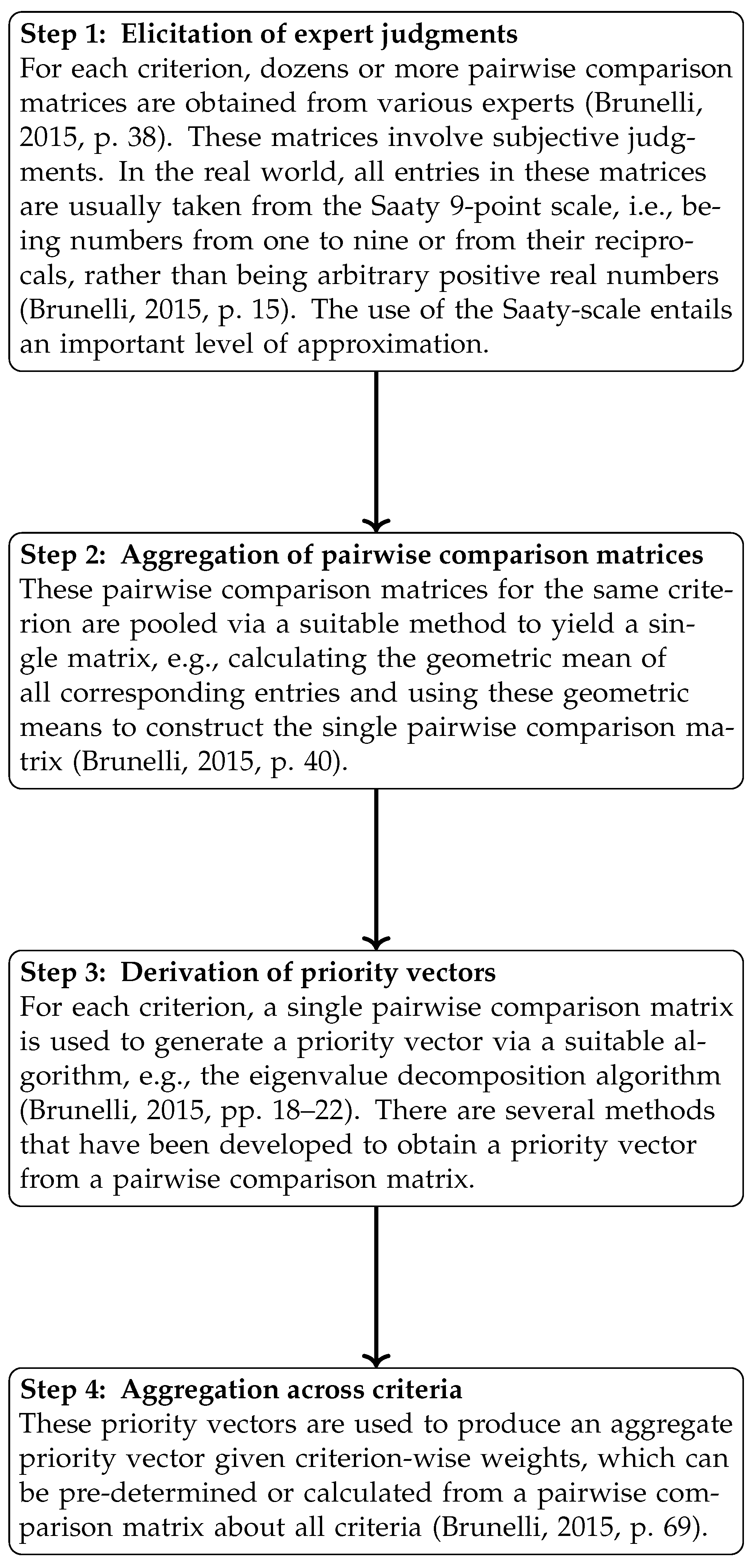
Figure 1. The four-step AHP procedure based on Brunelli (2015) [12].
Axioms 14 00860 g001
Figure 2. The convex hulls of three option pairs from the Belton–Gear example. In each plot, the triangle with black solid sides is T in (14), and the dashed line is the angle bisector B in (15). The left convex hull (triangle with solid red sides) is for the three points in (34), the middle one (green sides) is for those in (35), and the right one (blue sides) is for those in (36). The feasibility of rank reversal corresponds to crossing the bisector of the convex hull.
Axioms 14 00860 g002
Figure 3. The convex hulls of option pairs arising from the four examples in (37), (44), (51), and (58). In each plot, the triangle with black solid sides is T in (14), and the dashed line is B in (15). Each row contains three convex hulls (triangles with solid colored sides) of one example. The convex hulls in (41)–(43) are in row 1 (from the left to the right). Similarly, those in (48)–(50) are in row 2, those in (55)–(57) are in row 3, and those in (62)–(64) are in row 4. Each column contains four convex hulls of one pair of options. The feasibility of rank reversal corresponds to crossing the bisector of the convex hull.
Axioms 14 00860 g003
Disclaimer/Publisher’s Note: The statements, opinions and data contained in all publications are solely those of the individual author(s) and contributor(s) and not of MDPI and/or the editor(s). MDPI and/or the editor(s) disclaim responsibility for any injury to people or property resulting from any ideas, methods, instructions or products referred to in the content.