Statistical Formulation for Average Parameter Determination via Quantile-Linked Auxiliary Characteristics

Abstract

This article suggests a brief and integrated methodology for enhancing the mean estimation in a finite population using the pre-specified median of the target variable in conjunction with quantile-related auxiliary measurements. Although a number of conventional ratio and regression estimators are reliant on the average of the auxiliary variable, the current study presents new exponential-type families that combine the variable’s known median under investigation with the dispersion-related characteristics of supplementary information. The estimators are constructed and analyzed theoretically, under Simple Random Sampling Without Replacement (SRSWOR), and the minimum expression of the MSE under optimal conditions is obtained. The results are confirmed using simulated Kumaraswamy–Gamma populations and through several real-world datasets, such as those on education, wheat production, U.S. cereal consumption, and solar radiation data (HI-SEAS weather station, September–December 2016). The findings consistently demonstrate that the developed estimators provide a substantially lower MSE and greater percentage relative efficiency (PRE) relative to conventional estimators. These applications indicate that the median-based unified framework can be used to give more precise and efficient mean estimation in several fields, comprising agriculture, nutrition, and education, as well as meteorological and environmental research.

1. Introduction

Sample surveys are very fundamental in research since they offer a convenient and useful method of gathering representative data from large groups. There are multiple methods of carrying out surveys, such as online questionnaires, face-to-face interviews, group surveys, or mailed or phone surveys. They are applied extensively in the various fields of education, healthcare, labor markets, business, agriculture, radiation, environmental studies, and energy research. The effectiveness of a survey’s data collection approach has a significant impact on its efficacy. Ill-conceived research can lead to an erroneous finding, but a well-crafted survey that employs the best statistical tools can lead to valid and solid findings. Adding more information to survey-based estimates in the form of auxiliary variables is one of the strategies that can be used to strengthen the survey-based estimates. To enhance the accuracy of estimates of study parameters, the addition of auxiliary variables to estimation procedures can go a long way (Alomair and Shahzad [1]).

Regression, ratio, or modified versions of these estimators are typically utilized when there is a favorable association between the supplementary variable X and the research variable Y. Under SRSWOR, these methods consistently outperform the conventional ones. Besides these methods, utilizing the median information regarding the research parameter provides yet another dimension in terms of the construction of efficient estimators. Using the known median in ratio-type or regression-type estimators, the precision of estimation in means can be improved further.

The arithmetic mean is one of the most popular summary measures in the scientific, social, and applied world. Due to the fact that mean estimation is the centerpiece of sampling theory, there has been a continuous effort to enhance its accuracy. Ratio and regression-based techniques have been extended to many studies. For example, Chutiman et al. [2] used linear transformations of auxiliary variables in layered sampling, Alomair and Shahzad [3] created modified regression estimators in the framework of median ranked set sampling, and Koc and Koc [4] developed more efficient mean estimators in the context of simple random sampling using quantile regression coefficients. Despite this development, the majority of current techniques mainly depend on the average of the auxiliary variables, and there has not been much research devoted to exploring the possibility of using the pre-specified median of the target variable as a basis for achieving efficiency gains. To fill this gap, it is essential to have a single framework that incorporates information such as the median along with supplementary variables to enhance the estimation of a population’s true mean value.

In this paper, we focus on the use of supplementary information, specifically, the pre-specified median of the target variable and the average of an auxiliary variable, to derive an innovative family of ratio exponential estimators. A known population median is often assumed in survey situations; median values are frequently available from previous censuses or administrative reports or summaries of categorized results. This is also feasible because in many cases, it is possible to identify the median without having the entire dataset, as it is sufficient to have grouped or frequency data. This assumption provides a unified theoretical framework for the proposed estimators that are mathematically tractable and allow for closed-form representations of bias and mean squared error (MSE). In order to illustrate realistic situations in which such an assumption applies, several applied cases are given below:

• In a university exam, the task was to estimate the average marks of 5000 students. The median marks, which fell between 60 and 75, were the only category provided.
• For 800 university faculty members, the aim was to estimate the average salary. The median salary (RMB 10,000) was known from categorized payroll bands provided by the HR department.
• In a hospital-based BMI survey of 350 patients, the median BMI (21.75) was known from categories ranging from underweight to very severely obese.
• In a blood pressure monitoring program with 202 patients, the median systolic pressure (104.5 mmHg) was assumed to be known from medical categories such as hypotension and hypertensive emergency.
• In a farming area, 1000 farmers produce wheat, and their wheat is pooled according to the number of quintals produced per acre. Government survey results indicate that the average yield per acre is 12 quintals. This is why calculating the median value helps estimate the yield per acre more accurately.
• A housing office of a city keeps records of 2500 houses pooled by valuation in the city. The median house price (USD 350,000) is made publicly available in the summaries of real estate data and can be used as a known value to estimate the average price.
• The categorical Air Quality Index (AQI) classes are frequently reported in air quality monitoring at 500 stations. The median AQI value obtained using these categories provides a good known value to estimate the mean levels of the AQI.
• As part of an income distribution study conducted on 3000 workers, administrative data categorizes workers by monthly income levels. A good example of known information, which can effectively be used to estimate average income levels, is the median income (USD 4000), which can be obtained either by conducting employment surveys or using payroll data.

Hence, the current paper constructs such a framework by creating new types of exponential ratio estimators that explicitly make use of the pre-specified median of the target variable as well as raw dispersion measures of auxiliary variables. The reason behind the motivation is that even though means or variances are frequently simpler to compute in practice than medians, they are not always available to the researcher, especially when the data are coded into groups or categories. In order to illustrate the usefulness of the constructed estimators, we provide examples of their applications in various areas, such as education, healthcare, agriculture, and nutrition, plus a real-life application to meteorological data on solar radiation collected at the HI-SEAS weather station. In the second usage, solar radiation (W/m²) is considered the response variable, and temperature (°F) is considered supplementary information. This not only emphasizes the generality of the new method, but it also serves to indicate its relevance to pressing environmental and energy-related studies.

The subsequent sections of this article are arranged as follows: Section 2 surveys the related literature on mean estimation using auxiliary information and identifies key gaps motivating this study. The Quantile-Linked Measures of Dispersion and Adapted Family Section introduces an adapted class of ratio exponential estimators based on pre-specified medians and auxiliary dispersion measures such as the interquartile range, semi-interquartile range, mid-range, and interdecile range. Section 3 extends this to a generalized exponential-type family, with analytical expressions for bias and MSE, including optimal parameter values for the minimum MSE. Section 4 evaluates estimator performance through simulation studies under Kumaraswamy–Gamma distributions and empirical applications to datasets from education, agriculture, nutrition, and solar radiation. Section 5 offers a conclusion.

2. Literature Review on Median-Oriented Studies and Adapted Family

Over the past few years, accurate estimates of population means and parameters have become increasingly important in research. One reason for studying this topic is that researchers aim to create useful and accurate estimators. Ref. [5] introduced a ratio estimator for the median parameter. The idea of applying the study variable’s median in a ratio-based estimator for the population mean, especially in situations lacking auxiliary variables, was first proposed by Subramani [6,7]. His estimator showed that utilizing the known features of the target variable can improve the results of estimation. Additionally, estimators that use the median are important because they handle outliers well and require less complete data to work accurately. Lamichhane et al. [8] improved the median-based method by developing a population average estimator utilizing the median of an additional variable. Irfan et al. [9] and Yusuf et al. [10] defined an improved class of median-based power-type mean estimators. They expanded on previous studies by recommending estimators that help reduce bias and mean squared error when samples are taken without replacement. Their suggested classes outperform traditional ratio and regression estimators, as well as those developed by Subramani [6,7], as supported by theoretical derivations and empirical analyses. Refs. [11,12] introduced exponential families of median-based estimators under SRSWOR, building on earlier works by Subramani [6,7] and Irfan et al. [9]. Their proposed estimators demonstrated better performance in terms of MSE and PRE. Empirical evidence confirmed that the constructed family of estimators consistently outperformed their traditional and contemporary counterparts, reinforcing the utility of median-based modifications in practical survey applications. Abdullahi and Ugwuowo [13] developed median-based regression-type mean estimators with two tuning parameters. Singh and Tiwari [14] defined median-based mean estimators with bivariate auxiliary information under the neutrosophic framework. Kurbah et al. [15] extended this study on median-based mean estimators with double ranked set sampling.

According to the literature, few studies have focused on creating mean estimators that use both median-based linear regression and a median-based exponential component. This gap underscores the motivation for the present study. Therefore, in the following subsection, we define an exponential family of adapted median-based mean estimators that utilize both of these study variable median-based components with known raw measures of dispersion from the auxiliary variable.

Quantile-Linked Measures of Dispersion and Adapted Family

This section defines a generalized family of median-based estimators for the mean parameter, specifically designed for situations where certain quantile-linked raw measures of dispersion related to an auxiliary variable are readily available. These estimators make use of simple statistical methods to enhance the estimation process under SRSWOR. The dispersion measures incorporated into the development of these estimators include the following:

• IQR:

  $$R_{iq}=Q_3\left(X\right)-Q_1\left(X\right)$$
• SIQR:

  $$R_{sq}={\displaystyle \frac{Q_3\left(X\right)-Q_1\left(X\right)}{2}}$$
• MR:

  $$R_{mid}={\displaystyle \frac{max\left(X\right)+min\left(X\right)}{2}}$$
• IDR:

  $$R_{id}=D_9\left(X\right)-D_1\left(X\right).$$

• Measuring the spread of data is crucial, and the interquartile range (IQR), semi-interquartile range (SIQR), mid-range (MR), and interdecile range (IDR) are among the most practical and widely used raw measures for this purpose (Soni and Pandey [16]; Naz et al. [17]). The values obtained from these metrics play a significant role in constructing new estimators for the population mean. When SRSWOR is used, population dispersion estimation accuracy is enhanced by the inclusion of crucial features of the auxiliary variable. The theoretical basis and statistical characteristics of these dispersion measures are well-researched topics in the academic literature.

By following the Cetin and Koyuncu [18,19,20] structure of estimators, we define the known median-based mean family of adapted estimators by including raw measures (IQR, SIQR, MR, IDR), as given below:

$${\widehat{Y}}_{Gi}=\left\{w_1{\widehat{\mu }}_y+w_2\left({\tilde{\mu }}_M-{\tilde{\mu }}_m\right)\right\}exp\left({\displaystyle \frac{a_1\left({\tilde{\mu }}_M-{\tilde{\mu }}_m\right)}{a_1\left({\tilde{\mu }}_M+{\tilde{\mu }}_m\right)+2b_1}}\right),$$

(1)

where $w_1$ and $w_2$ correspond to optimally defined constants. $({\widehat{\mu }}_y,{\tilde{\mu }}_m)$ denote the sample mean and median of the response variable (Y), respectively. ${\tilde{\mu }}_M$ is the population median of (Y). Further, $a_1$ and $b_1$ are either raw measures of the dispersion of the auxiliary variable (X) or unity. It is worth noting that the exponential formulation is based on Shahzad et al. [11], who revealed that exponential ratio-type structures provide lower bias and more stable MSE when the variables in the survey are positively correlated. The current research extends this argument further by anchoring quantile-related and dispersion metrics to exponential-type estimators.

The lowest MSE of ${\widehat{Y}}_{Gi}$ achieved under optimum settings,

$$w_1^{\left(opt\right)}={\displaystyle \frac{8-\lambda {\theta }^2{\tilde{C}}_M^2}{8\left\{1+\lambda C_y^2\left(1-r_{ym}^2\right)\right\}}}\mathrm{and}$$

$$w_2^{\left(opt\right)}={\displaystyle \frac{{\mu }_y\left[\lambda {\theta }^3{\tilde{C}}_M^3+8C_y{r}_{ym}-\lambda {\theta }^2{\tilde{C}}_M^2{C}_y{r}_{ym}-4\theta {\tilde{C}}_M\left\{1-\lambda C_y^2\left(1-r_{ym}^2\right)\right\}\right]}{8{\tilde{\mu }}_M{\tilde{C}}_M\left\{1+\lambda C_y^2\left(1-r_{ym}^2\right)\right\}}},$$

is given by

$$MS{E}_{min}\left({\widehat{Y}}_{Gi}\right)={\displaystyle \frac{\lambda {\mu }_y^2\left\{64C_y^2\left(1-r_{ym}^2\right)-\lambda {\theta }^4{\tilde{C}}_M^4-16\lambda {\theta }^2{\tilde{C}}_M^2{C}_y^2\left(1-r_{ym}^2\right)\right\}}{64\left\{1+\lambda C_y^2\left(1-r_{ym}^2\right)\right\}}}$$

(2)

where $\lambda ={\displaystyle \frac{1-f}{n}}$, $f={\displaystyle \frac{n}{N}}$, and $\theta ={\displaystyle \frac{a_1{\mu }_M}{a_1{\mu }_M+b_1}}$. All details of the estimator family are listed in

Table 1. Members of adapted family.

Estimator	Values of Constants
	${\mathit{a}}_{\mathbf{1}}$	${\mathit{b}}_{\mathbf{1}}$
${\widehat{Y}}_{G1}=\left\{w_1{\widehat{\mu }}_y+w_2\left({\tilde{\mu }}_M-{\tilde{\mu }}_m\right)\right\}exp\left({\displaystyle \frac{{\tilde{\mu }}_M-{\tilde{\mu }}_m}{{\tilde{\mu }}_M+{\tilde{\mu }}_m+2R_{mid}}}\right)$	1	$R_{mid}$
${\widehat{Y}}_{G2}=\left\{w_1{\widehat{\mu }}_y+w_2\left({\tilde{\mu }}_M-{\tilde{\mu }}_m\right)\right\}exp\left({\displaystyle \frac{{\tilde{\mu }}_M-{\tilde{\mu }}_m}{{\tilde{\mu }}_M+{\tilde{\mu }}_m+2R_{id}}}\right)$	1	$R_{id}$
${\widehat{Y}}_{G3}=\left\{w_1{\widehat{\mu }}_y+w_2\left({\tilde{\mu }}_M-{\tilde{\mu }}_m\right)\right\}exp\left({\displaystyle \frac{{\tilde{\mu }}_M-{\tilde{\mu }}_m}{{\tilde{\mu }}_M+{\tilde{\mu }}_m+2R_{iq}}}\right)$	1	$R_{iq}$
${\widehat{Y}}_{G4}=\left\{w_1{\widehat{\mu }}_y+w_2\left({\tilde{\mu }}_M-{\tilde{\mu }}_m\right)\right\}exp\left({\displaystyle \frac{{\tilde{\mu }}_M-{\tilde{\mu }}_m}{{\tilde{\mu }}_M+{\tilde{\mu }}_m+2R_{sq}}}\right)$	1	$R_{sq}$
${\widehat{Y}}_{G5}=\left\{w_1{\widehat{\mu }}_y+w_2\left({\tilde{\mu }}_M-{\tilde{\mu }}_m\right)\right\}exp\left({\displaystyle \frac{R_{mid}\left({\tilde{\mu }}_M-{\tilde{\mu }}_m\right)}{R_{mid}\left({\tilde{\mu }}_M+{\tilde{\mu }}_m\right)+2}}\right)$	$R_{mid}$	1
${\widehat{Y}}_{G6}=\left\{w_1{\widehat{\mu }}_y+w_2\left({\tilde{\mu }}_M-{\tilde{\mu }}_m\right)\right\}exp\left({\displaystyle \frac{R_{id}\left({\tilde{\mu }}_M-{\tilde{\mu }}_m\right)}{R_{id}\left({\tilde{\mu }}_M+{\tilde{\mu }}_m\right)+2}}\right)$	$R_{id}$	1
${\widehat{Y}}_{G7}=\left\{w_1{\widehat{\mu }}_y+w_2\left({\tilde{\mu }}_M-{\tilde{\mu }}_m\right)\right\}exp\left({\displaystyle \frac{R_{iq}\left({\tilde{\mu }}_M-{\tilde{\mu }}_m\right)}{R_{iq}\left({\tilde{\mu }}_M+{\tilde{\mu }}_m\right)+2}}\right)$	$R_{iq}$	1
${\widehat{Y}}_{G8}=\left\{w_1{\widehat{\mu }}_y+w_2\left({\tilde{\mu }}_M-{\tilde{\mu }}_m\right)\right\}exp\left({\displaystyle \frac{R_{sq}\left({\tilde{\mu }}_M-{\tilde{\mu }}_m\right)}{R_{sq}\left({\tilde{\mu }}_M+{\tilde{\mu }}_m\right)+2}}\right)$	$R_{sq}$	1

, where $a_1$ and $b_1$ are chosen constants in light of references [16,17].

3. Generalized Family of Median-Based Mean Estimators Using Raw Dispersion Measures

It is well known that ratio [21], regression [22,23], and exponential [24,25] methods are useful for estimating the mean parameter in survey sampling when a correlation exists between the supplementary and study variables. Building on mid-nineteenth-century developments, these techniques are now vital in statistics. Their use began in agriculture and later expanded to other industries. Although linear regression with the known mean of (X) is widely used, the current literature shows that not many studies have considered using both the median of the target variable and the mean of the supplementary information at the same time. Because of this gap, more research in this area is required. Using Alharbi et al.’s [26] framework, we can form a difference-based estimator for the average parameter utilizing both the median of the target variable and the mean of the auxiliary variable:

$${\widehat{Y}}_p={\varpi }_a{\widehat{\mu }}_y+{\varpi }_b\left({\tilde{\mu }}_M-{\tilde{\mu }}_m\right)+{\varpi }_c\left({\widehat{\mu }}_x-{\mu }_x\right),$$

(3)

where ${\varpi }_a,{\varpi }_b,{\varpi }_c$ are suitably chosen constants.

Following ${\widehat{Y}}_{Gi}$ and ${\widehat{Y}}_p$, we formulate a generalized class of median-based mean estimators ${\widehat{Y}}_{pi}$ using raw dispersion measures, given by

$${\widehat{Y}}_{pi}=\left\{{\varpi }_a{\widehat{\mu }}_y+{\varpi }_b\left({\tilde{\mu }}_M-{\tilde{\mu }}_m\right)+{\varpi }_c\left({\widehat{\mu }}_x-{\mu }_x\right)\right\}exp\left({\displaystyle \frac{a_1\left({\tilde{\mu }}_M-{\tilde{\mu }}_m\right)}{a_1\left({\tilde{\mu }}_M+{\tilde{\mu }}_m\right)+2b_1}}\right),$$

(4)

where $a_1$ and $b_1$ are as explained earlier, and $({\widehat{\mu }}_x,{\mu }_x)$ are the sample and population means of (X), respectively. Some members of the generalized family of median-based mean estimators ${\widehat{Y}}_{pi}$ are provided in

Table 2. Members of proposed family.

Estimator	Values of Constants
	${\mathit{a}}_{\mathbf{1}}$	${\mathit{b}}_{\mathbf{1}}$
${\widehat{Y}}_{p1}=\left\{{\varpi }_a{\widehat{\mu }}_y+{\varpi }_b\left({\tilde{\mu }}_M-{\tilde{\mu }}_m\right)+{\varpi }_c\left({\widehat{\mu }}_x-{\mu }_x\right)\right\}exp\left({\displaystyle \frac{{\tilde{\mu }}_M-{\tilde{\mu }}_m}{{\tilde{\mu }}_M+{\tilde{\mu }}_m+2R_{mid}}}\right)$	1	$R_{mid}$
${\widehat{Y}}_{p2}=\left\{{\varpi }_a{\widehat{\mu }}_y+{\varpi }_b\left({\tilde{\mu }}_M-{\tilde{\mu }}_m\right)+{\varpi }_c\left({\widehat{\mu }}_x-{\mu }_x\right)\right\}exp\left({\displaystyle \frac{{\tilde{\mu }}_M-{\tilde{\mu }}_m}{{\tilde{\mu }}_M+{\tilde{\mu }}_m+2R_{id}}}\right)$	1	$R_{id}$
${\widehat{Y}}_{p3}=\left\{{\varpi }_a{\widehat{\mu }}_y+{\varpi }_b\left({\tilde{\mu }}_M-{\tilde{\mu }}_m\right)+{\varpi }_c\left({\widehat{\mu }}_x-{\mu }_x\right)\right\}exp\left({\displaystyle \frac{{\tilde{\mu }}_M-{\tilde{\mu }}_m}{{\tilde{\mu }}_M+{\tilde{\mu }}_m+2R_{iq}}}\right)$	1	$R_{iq}$
${\widehat{Y}}_{p4}=\left\{{\varpi }_a{\widehat{\mu }}_y+{\varpi }_b\left({\tilde{\mu }}_M-{\tilde{\mu }}_m\right)+{\varpi }_c\left({\widehat{\mu }}_x-{\mu }_x\right)\right\}exp\left({\displaystyle \frac{{\tilde{\mu }}_M-{\tilde{\mu }}_m}{{\tilde{\mu }}_M+{\tilde{\mu }}_m+2R_{sq}}}\right)$	1	$R_{sq}$
${\widehat{Y}}_{p5}=\left\{{\varpi }_a{\widehat{\mu }}_y+{\varpi }_b\left({\tilde{\mu }}_M-{\tilde{\mu }}_m\right)+{\varpi }_c\left({\widehat{\mu }}_x-{\mu }_x\right)\right\}exp\left({\displaystyle \frac{R_{mid}\left({\tilde{\mu }}_M-{\tilde{\mu }}_m\right)}{R_{mid}\left({\tilde{\mu }}_M+{\tilde{\mu }}_m\right)+2}}\right)$	$R_{mid}$	1
${\widehat{Y}}_{p6}=\left\{{\varpi }_a{\widehat{\mu }}_y+{\varpi }_b\left({\tilde{\mu }}_M-{\tilde{\mu }}_m\right)+{\varpi }_c\left({\widehat{\mu }}_x-{\mu }_x\right)\right\}exp\left({\displaystyle \frac{R_{id}\left({\tilde{\mu }}_M-{\tilde{\mu }}_m\right)}{R_{id}\left({\tilde{\mu }}_M+{\tilde{\mu }}_m\right)+2}}\right)$	$R_{id}$	1
${\widehat{Y}}_{p7}=\left\{{\varpi }_a{\widehat{\mu }}_y+{\varpi }_b\left({\tilde{\mu }}_M-{\tilde{\mu }}_m\right)+{\varpi }_c\left({\widehat{\mu }}_x-{\mu }_x\right)\right\}exp\left({\displaystyle \frac{R_{iq}\left({\tilde{\mu }}_M-{\tilde{\mu }}_m\right)}{R_{iq}\left({\tilde{\mu }}_M+{\tilde{\mu }}_m\right)+2}}\right)$	$R_{iq}$	1
${\widehat{Y}}_{p8}=\left\{{\varpi }_a{\widehat{\mu }}_y+{\varpi }_b\left({\tilde{\mu }}_M-{\tilde{\mu }}_m\right)+{\varpi }_c\left({\widehat{\mu }}_x-{\mu }_x\right)\right\}exp\left({\displaystyle \frac{R_{sq}\left({\tilde{\mu }}_M-{\tilde{\mu }}_m\right)}{R_{sq}\left({\tilde{\mu }}_M+{\tilde{\mu }}_m\right)+2}}\right)$	$R_{sq}$	1

using different choices of $a_1$ and $b_1$. All exponential formulations of estimators presented in Table 1 and Table 2 are expressed in a ratio-type form such that any homogeneous change in the measurement unit of (X) or (Y) has no effect on the estimator, making scale and unit invariance practically achievable.

Let

$${\xi }_a={\displaystyle \frac{{\widehat{\mu }}_y-{\mu }_y}{{\mu }_y}},{\xi }_b={\displaystyle \frac{{\tilde{\mu }}_m-{\tilde{\mu }}_M}{{\tilde{\mu }}_M}},{\xi }_c={\displaystyle \frac{{\widehat{\mu }}_x-{\mu }_x}{{\mu }_x}},$$

such that $E\left({\xi }_a\right)=E\left({\xi }_b\right)=E\left({\xi }_c\right)=0$. Further,

$$E\left({\xi }_a^2\right)=\lambda C_y^2,E\left({\xi }_b^2\right)=\lambda {\tilde{C}}_M^2,E\left({\xi }_c^2\right)=\lambda C_x^2,E\left({\xi }_a{\xi }_b\right)=\lambda r_{ym}{C}_y{\tilde{C}}_M,$$

$$E\left({\xi }_a{\xi }_c\right)=\lambda r_{yx}{C}_y{C}_x,\mathrm{and}E\left({\xi }_b{\xi }_c\right)=\lambda r_{mx}{\tilde{C}}_M{C}_x.$$

From Equation (4), rewriting ${\widehat{Y}}_{pi}$ in terms of ${\xi }_a$, ${\xi }_b$, and ${\xi }_c$, we get

$${\widehat{Y}}_{pi}=\left\{{\varpi }_a{\mu }_y(1+{\xi }_a)-{\varpi }_b{\tilde{\mu }}_M{\xi }_b-{\varpi }_c{\mu }_x{\xi }_c\right\}\left\{1-{\displaystyle \frac{\theta {\xi }_b}{2}}+{\displaystyle \frac{3{\theta }^2{\xi }_b^2}{8}}+\cdots \right\}.$$

(5)

By expanding Equation (5) and keeping terms only up to order two in $\xi$s, we can write

$$\begin{array}{cc}\hfill \left({\widehat{Y}}_{pi}-{\mu }_y\right)& =-{\mu }_y+{\mu }_y{\varpi }_a+{\mu }_y{\xi }_a{\varpi }_a-{\displaystyle \frac{1}{2}}{\mu }_y\theta {\xi }_b{\varpi }_a-{\tilde{\mu }}_M{\xi }_b{\varpi }_b-{\mu }_x{\xi }_c{\varpi }_c-{\displaystyle \frac{1}{2}}{\mu }_y\theta {\xi }_a{\xi }_b{\varpi }_a\hfill \\ \hfill & +{\displaystyle \frac{3}{8}}{\mu }_y{\theta }^2{\xi }_b^2{\varpi }_a+{\displaystyle \frac{1}{2}}{\tilde{\mu }}_M\theta {\xi }_b^2{\varpi }_b+{\displaystyle \frac{1}{2}}{\mu }_x\theta {\xi }_b{\xi }_c{\varpi }_c.\hfill \end{array}$$

(6)

From Equation (6)’s expectation applicability,

$$\begin{array}{cc}\hfill Bias\left({\widehat{Y}}_{pi}\right)& \cong {\displaystyle \frac{1}{8}}\left[-8{\mu }_y+4\lambda \theta {\tilde{C}}_M\left({\tilde{\mu }}_M{\tilde{C}}_M{\varpi }_b+{\mu }_x{C}_x{\varpi }_c{r}_{mx}\right)+{\mu }_y{\varpi }_a\left\{8+\lambda \theta {\tilde{C}}_M\left(3\theta {\tilde{C}}_M-4C_y{r}_{ym}\right)\right\}\right],\hfill \end{array}$$

(7)

$$\begin{array}{cc}\hfill MSE\left({\widehat{Y}}_{pi}\right)& \cong {\mu }_y^2+\lambda {\tilde{\mu }}_M{\tilde{C}}_M^2{\varpi }_b\left(-{\mu }_y\theta +{\tilde{\mu }}_M{\varpi }_b\right)+\lambda {\mu }_x^2{C}_x^2{\varpi }_c^2\hfill \\ \hfill & +\lambda {\mu }_x{\tilde{C}}_M{C}_x\left(-{\mu }_y\theta +2{\tilde{\mu }}_M{\varpi }_b\right){\varpi }_c{r}_{mx}+{\mu }_y^2{\varpi }_a^2\left[1+\lambda \left\{C_y^2+\theta {\tilde{C}}_M\left(\theta {\tilde{C}}_M-2C_y{r}_{ym}\right)\right\}\right]\hfill \\ \hfill & +{\displaystyle \frac{1}{4}}{\mu }_y{\varpi }_a\left[-8{\mu }_y+\lambda {\tilde{C}}_M\left\{\theta {\tilde{C}}_M\left(-3{\mu }_y\theta +8{\tilde{\mu }}_M{\varpi }_b\right)+8{\mu }_x\theta C_x{\varpi }_c{r}_{mx}\right.\right.\hfill \\ \hfill & \left.\left.+4C_y\left({\mu }_y\theta -2{\tilde{\mu }}_M{\varpi }_b\right)r_{ym}\right\}-8{\mu }_x\lambda C_y{C}_x{\varpi }_c{r}_{yx}\right].\hfill \end{array}$$

(8)

By minimizing Equation (8), the optimum versions of ${\varpi }_a,{\varpi }_b$, and ${\varpi }_c$ are

$${\varpi }_a^{\left(opt\right)}={\displaystyle \frac{8-\lambda {\theta }^2{\tilde{C}}_M^2}{8\left\{1+\lambda C_y^2\left(1-Q_{y,mx}^2\right)\right\}}},$$

$${\varpi }_b^{\left(opt\right)}={\displaystyle \frac{{\mu }_y\left[\begin{array}{cc}\hfill & \lambda {\theta }^3{\tilde{C}}_M^3(-1+r_{mx}^2)+(-8C_y+\lambda {\theta }^2{\tilde{C}}_M^2{C}_y)(r_{ym}-r_{mx}{r}_{yx})\hfill \\ \hfill & +4\theta {\tilde{C}}_M(-1+r_{mx}^2)\left\{-1+\lambda C_y^2(1-Q_{y,mx}^2)\right\}\hfill \end{array}\right]}{8{\tilde{\mu }}_M{\tilde{C}}_M(-1+r_{mx}^2)\left\{1+\lambda C_y^2(1-Q_{y,mx}^2)\right\}}},$$

$${\varpi }_c^{\left(opt\right)}={\displaystyle \frac{{\mu }_y(8-\lambda {\theta }^2{\tilde{C}}_M^2)C_y(r_{mx}{r}_{ym}-r_{yx})}{8{\mu }_x{C}_x(-1+r_{mx}^2)\left\{1+\lambda C_y^2(1-Q_{y,mx}^2)\right\}}},$$

where

$$Q_{y,mx}^2={\displaystyle \frac{r_{ym}^2+r_{yx}^2-2r_{ym}{r}_{yx}{r}_{mx}}{1-r_{mx}^2}}$$

is the coefficient of multiple determination with range [0,1] (Lamichhane et al. [8]). Further, $(C_y,C_x)$ are the coefficients of variation of Y and X, respectively. The correlation between $({\widehat{\mu }}_y,{\tilde{\mu }}_m)$ is $r_{ym}$, $({\widehat{\mu }}_y,{\widehat{\mu }}_x)$ is $r_{yx}$, and $({\tilde{\mu }}_m,{\widehat{\mu }}_x)$ is $r_{mx}$. Following Lamichhane et al. [8], ${\tilde{C}}_M={\displaystyle \frac{Cov({\widehat{\mu }}_y,{\tilde{\mu }}_m)}{{\mu }_y{\tilde{\mu }}_M}}$.

We substitute the optimum values of ${\varpi }_a$, ${\varpi }_b$, and ${\varpi }_c$ in Equation (8), and after some simplifications, we get the minimum MSE of ${\widehat{Y}}_{pi}$, given by

$$MS{E}_{min}\left({\widehat{Y}}_{pi}\right)={\displaystyle \frac{\lambda {\mu }_y^2\left\{64C_y^2(1-Q_{y,mx}^2)-\lambda {\theta }^4{\tilde{C}}_M^4-16\lambda {\theta }^2{\tilde{C}}_M^2{C}_y^2(1-Q_{y,mx}^2)\right\}}{64\left\{1+\lambda C_y^2(1-Q_{y,mx}^2)\right\}}}.$$

(9)

Finally, comparing $MS{E}_{min}\left({\widehat{Y}}_{pi}\right)$<$MS{E}_{min}\left({\widehat{Y}}_{Gi}\right)$, we immediately observe the following efficiency condition:

$${\displaystyle \frac{\lambda {\mu }_y^2{C}_y^2{\left(r_{yx}-r_{ym}{r}_{mx}\right)}^2{\left(-8+\lambda {\theta }^2{\tilde{C}}_M^2\right)}^2}{64(1-r_{mx}^2)\left[1+\lambda C_y^2(1-r_{ym}^2)\right]\left[1+\lambda C_y^2(1-Q_{y,mx}^2)\right]}}>0.$$

Note that the exponential ratio-type estimators (${\widehat{Y}}_{Gi},{\widehat{Y}}_p$) are recommended for use only when X and Y exhibit a positive association. At a value of $r_{yx}$ above zero, the constructed expressions of the minimum MSE are always strictly non-negative, as expected theoretically. Further, the proposed method assumes a pre-specified median of the target variable and the raw dispersion values of the supplementary variable. If these quantities are unknown or only partially known, the method can be modified by substituting the required parameters with their corresponding sample values, which can be obtained through pilot surveys, historical data, or supplementary registers.

4. Numerical Illustration

4.1. Simulation Study

In our simulation experiment, we initially produced an X of size N = 100 by drawing from a Uniform(0,1) distribution. Then we defined the four parameters associated with the Kumaraswamy–Gamma distribution, namely the following: the Gamma shape of Kumaraswamy denoted by $\alpha$, the Gamma scale of Kumaraswamy denoted by $\beta$, and finally the two shape parameters a and b of Kumaraswamy. We subsequently generated Y using the inverse cumulative distribution (quantile) method, where the same Uniform(0,1) sequence was employed to induce dependence between X and Y. Thus, we used the same Uniform(0,1) and used the inverse Kumaraswamy cumulative distribution function,

$$w={[1-{(1-u)}^{1/b}]}^{1/a},$$

so that the probability of w is expressed by the Gamma CDF $G{\left(x\right)}^a$, and G indicates the Gamma CDF. We determined Y by taking the inverse of the Gamma CDF:

$$Y=G^{-1}\left(w\right)=\mathtt{qgamma}(w,\mathrm{shape}=\alpha ,\mathrm{scale}=\beta ).$$

Therefore, Y is a strictly increasing transform of the same u that defines X, which ensures $Cov(X,Y)>0$. The induced associations of X and Y in the three simulated populations were around 0.94, 0.96, and 0.97, which support the strong positive dependence required by the ratio exponential estimators.

With the application of the Kumaraswamy–Gamma model, the pair of $\left\{(X_i,Y_i)\right\}$ is obtained. For more details about Kumaraswamy–Gamma, see [27,28]. The three datasets were generated using the Kumaraswamy–Gamma model, each with different parameter values, as follows:

• For Simulated Population-1:
  $\alpha =2.0,\beta =1.0,a=1.5,b=2.0.$
• For Simulated Population-2:
  $\alpha =3.0,\beta =1.5,a=2.0,b=3.0.$
• For Simulated Population-3:
  $\alpha =4.0,\beta =2.0,a=3.0,b=4.0.$

Interpretation of Simulated Population Results (Table 3, Table 4, Table 5 and Table 6)

• Substantial reduction in MSE with ${\widehat{Y}}_{pi}$ estimators:
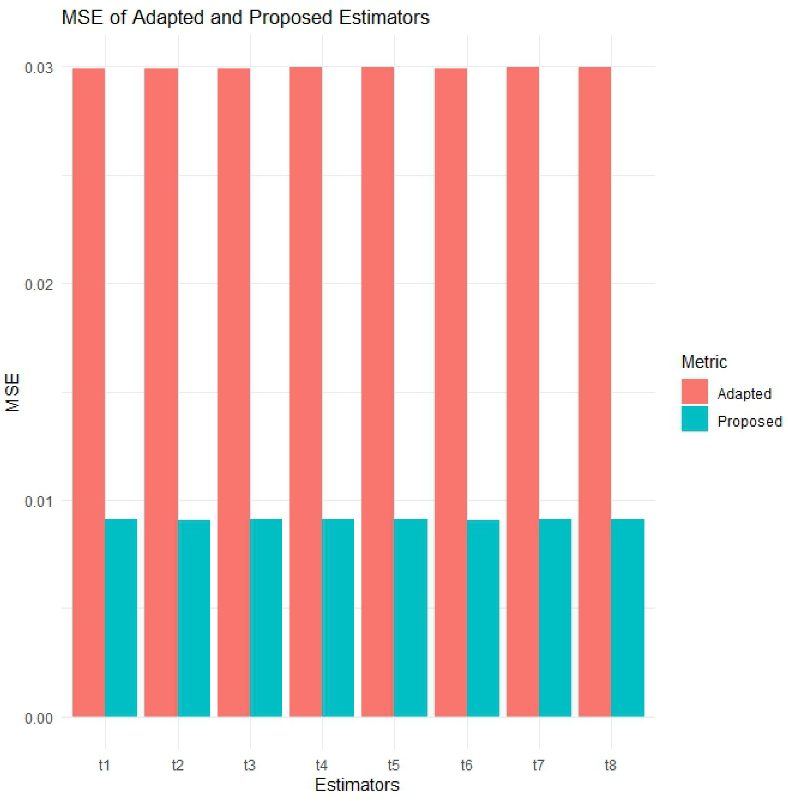
  The ${\widehat{Y}}_{pi}$ (developed) estimators consistently achieve significantly smaller MSE values compared to the traditional estimators ${\widehat{Y}}_{G1}$ to ${\widehat{Y}}_{G8}$. For instance, in Simulated Population-1, ${\widehat{Y}}_{Gi}$ estimators have MSEs around 0.0299 (e.g., ${\widehat{Y}}_{G1}$ = 0.02992718), whereas ${\widehat{Y}}_{pi}$ estimators are around 0.0090 (e.g., ${\widehat{Y}}_{p1}$ = 0.009089002). This demonstrates an approximately 70% reduction in estimation error, indicating the improved accuracy of the proposed TP method.
• Consistency and robustness across populations:
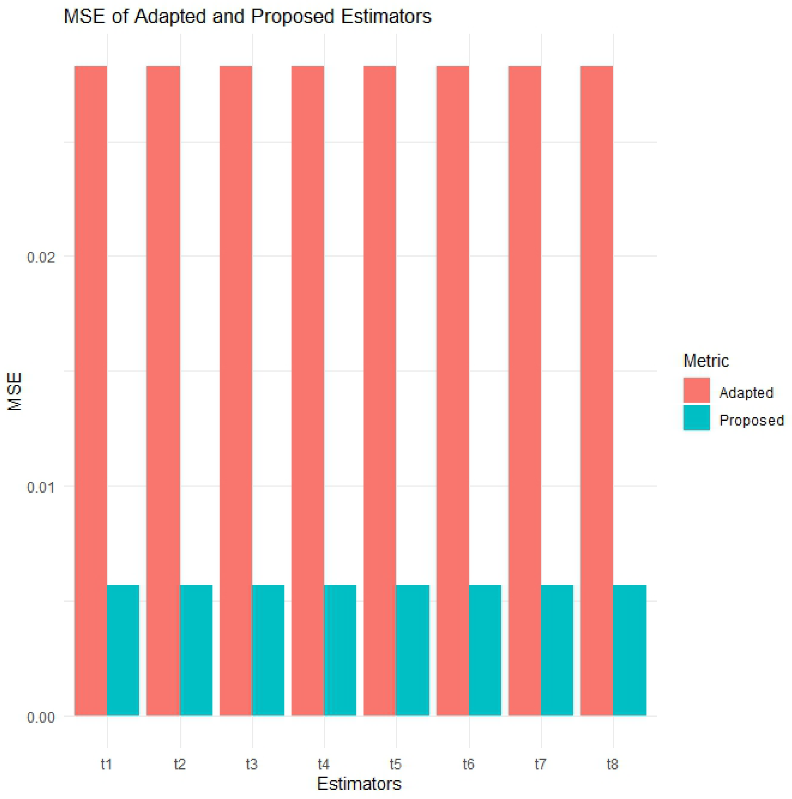
  ${\widehat{Y}}_{pi}$ estimators are very consistent in all three populations. In Simulated Population-2, ${\widehat{Y}}_{pi}$ MSEs are tightly grouped around 0.00568 (e.g., ${\widehat{Y}}_{p3}$ = 0.005681118; ${\widehat{Y}}_{p5}$ = 0.005681200), while ${\widehat{Y}}_{Gi}$ estimators vary slightly more, around 0.02824 (e.g., ${\widehat{Y}}_{G5}$ = 0.02824520). This suggests that ${\widehat{Y}}_{pi}$ methods are more robust to changes in data structure or distribution.
• Lowest MSE achieved:
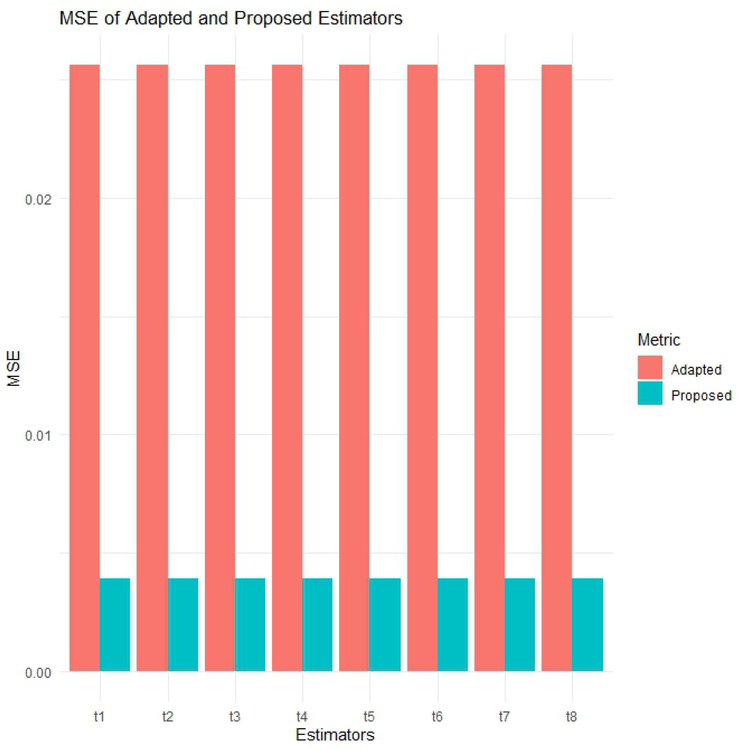
  The lowest MSE of all three estimators (in Population-1 and Population-3) is seen in Population-3, which implies that Population-3 has better properties for desirable mean estimation. To illustrate, the MSE of ${\widehat{Y}}_{p3}$ in Population-3 is 0.003936279, whereas that of ${\widehat{Y}}_{G3}$ is 0.02560332. This indicates a significant difference and a lower overall error floor in Population-3. This trend points to the effect of population characteristics on estimators.
• Highest PRE achieved:
  The ${\widehat{Y}}_{pi}$ (proposed) estimators consistently yield significantly higher PRE values compared to the adapted estimators ${\widehat{Y}}_{G1}$ to ${\widehat{Y}}_{G8}$ in all three simulated populations. Note that PRE was calculated as the ratio of the MSE of a baseline estimator to that of the corresponding estimator under comparison, multiplied by 100. The proposed estimators were compared against all the adapted ones to perform a thorough efficiency analysis.
• Dependence between X and Y:
  In practice, there is high positive correlation between these simulated populations. Using the parameter sets of the three simulated populations, the actual correlations are around 0.94, 0.95, and 0.97, respectively. Such values verify the fact that the reported PRE gains are actually due to the nonzero auxiliary information correlation instead of noise.

Table 3. MSE for simulated datasets.

$\widehat{\mathit{\theta }}$	SP-1	SP-2	SP-3
${\widehat{Y}}_{G1}$	0.02992718	0.02824489	0.02560332
${\widehat{Y}}_{G2}$	0.02990457	0.02823964	0.02560211
${\widehat{Y}}_{G3}$	0.02992718	0.02824489	0.02560332
${\widehat{Y}}_{G4}$	0.02994235	0.02824922	0.02560441
${\widehat{Y}}_{G5}$	0.02992912	0.02824520	0.02560338
${\widehat{Y}}_{G6}$	0.02990606	0.02823983	0.02560214
${\widehat{Y}}_{G7}$	0.02992911	0.02824520	0.02560338
${\widehat{Y}}_{G8}$	0.02994434	0.02824960	0.02560449
${\widehat{Y}}_{p1}$	0.009089002	0.005681118	0.003936279
${\widehat{Y}}_{p2}$	0.009081033	0.005679691	0.003935994
${\widehat{Y}}_{p3}$	0.009089002	0.005681118	0.003936279
${\widehat{Y}}_{p4}$	0.009094189	0.005682264	0.003936531
${\widehat{Y}}_{p5}$	0.009089670	0.005681200	0.003936292
${\widehat{Y}}_{p6}$	0.009081566	0.005679743	0.003936002
${\widehat{Y}}_{p7}$	0.009089670	0.005681200	0.003936292
${\widehat{Y}}_{p8}$	0.009094859	0.005682364	0.003936549

Table 3. MSE for simulated datasets.

$\widehat{\mathit{\theta }}$	SP-1	SP-2	SP-3
${\widehat{Y}}_{G1}$	0.02992718	0.02824489	0.02560332
${\widehat{Y}}_{G2}$	0.02990457	0.02823964	0.02560211
${\widehat{Y}}_{G3}$	0.02992718	0.02824489	0.02560332
${\widehat{Y}}_{G4}$	0.02994235	0.02824922	0.02560441
${\widehat{Y}}_{G5}$	0.02992912	0.02824520	0.02560338
${\widehat{Y}}_{G6}$	0.02990606	0.02823983	0.02560214
${\widehat{Y}}_{G7}$	0.02992911	0.02824520	0.02560338
${\widehat{Y}}_{G8}$	0.02994434	0.02824960	0.02560449
${\widehat{Y}}_{p1}$	0.009089002	0.005681118	0.003936279
${\widehat{Y}}_{p2}$	0.009081033	0.005679691	0.003935994
${\widehat{Y}}_{p3}$	0.009089002	0.005681118	0.003936279
${\widehat{Y}}_{p4}$	0.009094189	0.005682264	0.003936531
${\widehat{Y}}_{p5}$	0.009089670	0.005681200	0.003936292
${\widehat{Y}}_{p6}$	0.009081566	0.005679743	0.003936002
${\widehat{Y}}_{p7}$	0.009089670	0.005681200	0.003936292
${\widehat{Y}}_{p8}$	0.009094859	0.005682364	0.003936549

Table 4. PRE for Simulated Population-1.

$\widehat{\mathit{\theta }}$	${\widehat{\mathit{Y}}}_{\mathit{p}1}$	${\widehat{\mathit{Y}}}_{\mathit{p}2}$	${\widehat{\mathit{Y}}}_{\mathit{p}3}$	${\widehat{\mathit{Y}}}_{\mathit{p}4}$	${\widehat{\mathit{Y}}}_{\mathit{p}5}$	${\widehat{\mathit{Y}}}_{\mathit{p}6}$	${\widehat{\mathit{Y}}}_{\mathit{p}7}$	${\widehat{\mathit{Y}}}_{\mathit{p}8}$
${\widehat{Y}}_{G1}$	329.2681	329.0193	329.2681	329.4349	329.2894	329.0357	329.2893	329.4568
${\widehat{Y}}_{G2}$	329.5571	329.3081	329.5570	329.7241	329.5783	329.3245	329.5783	329.7459
${\widehat{Y}}_{G3}$	329.2681	329.0194	329.2681	329.4350	329.2894	329.0358	329.2894	329.4568
${\widehat{Y}}_{G4}$	329.0803	328.8317	329.0803	329.2470	329.1015	328.8481	329.1015	329.2689
${\widehat{Y}}_{G5}$	329.2439	328.9952	329.2439	329.4107	329.2652	329.0115	329.2651	329.4326
${\widehat{Y}}_{G6}$	329.5377	329.2887	329.5377	329.7047	329.5590	329.3051	329.5590	329.7266
${\widehat{Y}}_{G7}$	329.2439	328.9952	329.2439	329.4108	329.2652	329.0116	329.2652	329.4326
${\widehat{Y}}_{G8}$	329.0560	328.8074	329.0560	329.2228	329.0773	328.8238	329.0773	329.2446

Table 4. PRE for Simulated Population-1.

$\widehat{\mathit{\theta }}$	${\widehat{\mathit{Y}}}_{\mathit{p}1}$	${\widehat{\mathit{Y}}}_{\mathit{p}2}$	${\widehat{\mathit{Y}}}_{\mathit{p}3}$	${\widehat{\mathit{Y}}}_{\mathit{p}4}$	${\widehat{\mathit{Y}}}_{\mathit{p}5}$	${\widehat{\mathit{Y}}}_{\mathit{p}6}$	${\widehat{\mathit{Y}}}_{\mathit{p}7}$	${\widehat{\mathit{Y}}}_{\mathit{p}8}$
${\widehat{Y}}_{G1}$	329.2681	329.0193	329.2681	329.4349	329.2894	329.0357	329.2893	329.4568
${\widehat{Y}}_{G2}$	329.5571	329.3081	329.5570	329.7241	329.5783	329.3245	329.5783	329.7459
${\widehat{Y}}_{G3}$	329.2681	329.0194	329.2681	329.4350	329.2894	329.0358	329.2894	329.4568
${\widehat{Y}}_{G4}$	329.0803	328.8317	329.0803	329.2470	329.1015	328.8481	329.1015	329.2689
${\widehat{Y}}_{G5}$	329.2439	328.9952	329.2439	329.4107	329.2652	329.0115	329.2651	329.4326
${\widehat{Y}}_{G6}$	329.5377	329.2887	329.5377	329.7047	329.5590	329.3051	329.5590	329.7266
${\widehat{Y}}_{G7}$	329.2439	328.9952	329.2439	329.4108	329.2652	329.0116	329.2652	329.4326
${\widehat{Y}}_{G8}$	329.0560	328.8074	329.0560	329.2228	329.0773	328.8238	329.0773	329.2446

Table 5. PRE for Simulated Population-2.

$\widehat{\mathit{\theta }}$	${\widehat{\mathit{Y}}}_{\mathit{p}1}$	${\widehat{\mathit{Y}}}_{\mathit{p}2}$	${\widehat{\mathit{Y}}}_{\mathit{p}3}$	${\widehat{\mathit{Y}}}_{\mathit{p}4}$	${\widehat{\mathit{Y}}}_{\mathit{p}5}$	${\widehat{\mathit{Y}}}_{\mathit{p}6}$	${\widehat{\mathit{Y}}}_{\mathit{p}7}$	${\widehat{\mathit{Y}}}_{\mathit{p}8}$
${\widehat{Y}}_{G1}$	497.1713	497.0789	497.1713	497.2476	497.1767	497.0823	497.1767	497.2543
${\widehat{Y}}_{G2}$	497.2962	497.2038	497.2962	497.3725	497.3017	497.2071	497.3016	497.3793
${\widehat{Y}}_{G3}$	497.1713	497.0790	497.1713	497.2476	497.1768	497.0823	497.1768	497.2544
${\widehat{Y}}_{G4}$	497.0710	496.9787	497.0710	497.1473	497.0764	496.9820	497.0764	497.1540
${\widehat{Y}}_{G5}$	497.1641	497.0717	497.1641	497.2403	497.1695	497.0750	497.1695	497.2471
${\widehat{Y}}_{G6}$	497.2917	497.1993	497.2916	497.3679	497.2971	497.2026	497.2971	497.3747
${\widehat{Y}}_{G7}$	497.1641	497.0717	497.1641	497.2403	497.1695	497.0750	497.1695	497.2471
${\widehat{Y}}_{G8}$	497.0622	496.9699	497.0622	497.1385	497.0677	496.9732	497.0677	497.1452

Table 5. PRE for Simulated Population-2.

$\widehat{\mathit{\theta }}$	${\widehat{\mathit{Y}}}_{\mathit{p}1}$	${\widehat{\mathit{Y}}}_{\mathit{p}2}$	${\widehat{\mathit{Y}}}_{\mathit{p}3}$	${\widehat{\mathit{Y}}}_{\mathit{p}4}$	${\widehat{\mathit{Y}}}_{\mathit{p}5}$	${\widehat{\mathit{Y}}}_{\mathit{p}6}$	${\widehat{\mathit{Y}}}_{\mathit{p}7}$	${\widehat{\mathit{Y}}}_{\mathit{p}8}$
${\widehat{Y}}_{G1}$	497.1713	497.0789	497.1713	497.2476	497.1767	497.0823	497.1767	497.2543
${\widehat{Y}}_{G2}$	497.2962	497.2038	497.2962	497.3725	497.3017	497.2071	497.3016	497.3793
${\widehat{Y}}_{G3}$	497.1713	497.0790	497.1713	497.2476	497.1768	497.0823	497.1768	497.2544
${\widehat{Y}}_{G4}$	497.0710	496.9787	497.0710	497.1473	497.0764	496.9820	497.0764	497.1540
${\widehat{Y}}_{G5}$	497.1641	497.0717	497.1641	497.2403	497.1695	497.0750	497.1695	497.2471
${\widehat{Y}}_{G6}$	497.2917	497.1993	497.2916	497.3679	497.2971	497.2026	497.2971	497.3747
${\widehat{Y}}_{G7}$	497.1641	497.0717	497.1641	497.2403	497.1695	497.0750	497.1695	497.2471
${\widehat{Y}}_{G8}$	497.0622	496.9699	497.0622	497.1385	497.0677	496.9732	497.0677	497.1452

Table 6. PRE for Simulated Population-3.

$\widehat{\mathit{\theta }}$	${\widehat{\mathit{Y}}}_{\mathit{p}1}$	${\widehat{\mathit{Y}}}_{\mathit{p}2}$	${\widehat{\mathit{Y}}}_{\mathit{p}3}$	${\widehat{\mathit{Y}}}_{\mathit{p}4}$	${\widehat{\mathit{Y}}}_{\mathit{p}5}$	${\widehat{\mathit{Y}}}_{\mathit{p}6}$	${\widehat{\mathit{Y}}}_{\mathit{p}7}$	${\widehat{\mathit{Y}}}_{\mathit{p}8}$
${\widehat{Y}}_{G1}$	650.4448	650.4141	650.4448	650.4726	650.4462	650.4149	650.4462	650.4745
${\widehat{Y}}_{G2}$	650.4918	650.4611	650.4918	650.5196	650.4933	650.4619	650.4932	650.5215
${\widehat{Y}}_{G3}$	650.4448	650.4141	650.4448	650.4726	650.4463	650.4149	650.4462	650.4745
${\widehat{Y}}_{G4}$	650.4031	650.3724	650.4031	650.4309	650.4045	650.3732	650.4045	650.4328
${\widehat{Y}}_{G5}$	650.4427	650.4120	650.4427	650.4704	650.4441	650.4128	650.4441	650.4724
${\widehat{Y}}_{G6}$	650.4906	650.4599	650.4906	650.5184	650.4920	650.4607	650.4920	650.5203
${\widehat{Y}}_{G7}$	650.4427	650.4120	650.4427	650.4705	650.4441	650.4128	650.4441	650.4724
${\widehat{Y}}_{G8}$	650.4002	650.3696	650.4002	650.4280	650.4017	650.3703	650.4017	650.4299

Table 6. PRE for Simulated Population-3.

$\widehat{\mathit{\theta }}$	${\widehat{\mathit{Y}}}_{\mathit{p}1}$	${\widehat{\mathit{Y}}}_{\mathit{p}2}$	${\widehat{\mathit{Y}}}_{\mathit{p}3}$	${\widehat{\mathit{Y}}}_{\mathit{p}4}$	${\widehat{\mathit{Y}}}_{\mathit{p}5}$	${\widehat{\mathit{Y}}}_{\mathit{p}6}$	${\widehat{\mathit{Y}}}_{\mathit{p}7}$	${\widehat{\mathit{Y}}}_{\mathit{p}8}$
${\widehat{Y}}_{G1}$	650.4448	650.4141	650.4448	650.4726	650.4462	650.4149	650.4462	650.4745
${\widehat{Y}}_{G2}$	650.4918	650.4611	650.4918	650.5196	650.4933	650.4619	650.4932	650.5215
${\widehat{Y}}_{G3}$	650.4448	650.4141	650.4448	650.4726	650.4463	650.4149	650.4462	650.4745
${\widehat{Y}}_{G4}$	650.4031	650.3724	650.4031	650.4309	650.4045	650.3732	650.4045	650.4328
${\widehat{Y}}_{G5}$	650.4427	650.4120	650.4427	650.4704	650.4441	650.4128	650.4441	650.4724
${\widehat{Y}}_{G6}$	650.4906	650.4599	650.4906	650.5184	650.4920	650.4607	650.4920	650.5203
${\widehat{Y}}_{G7}$	650.4427	650.4120	650.4427	650.4705	650.4441	650.4128	650.4441	650.4724
${\widehat{Y}}_{G8}$	650.4002	650.3696	650.4002	650.4280	650.4017	650.3703	650.4017	650.4299

4.2. Real-Life Applications

• Education data:
• Researchers in education must accurately determine how much is invested in education to make fair and effective decisions. The relationship between public education spending per person and personal income per person is typically quite clear. Estimating the means of these variables reveals what influences educational spending in various parts of the world. Reliable estimation is essential when analyzing datasets such as the Education dataset, originally compiled for modeling public spending on education (Chatterjee and Hadi, [29]). The robustbase package in R software (Ref. [30]) includes this dataset, with per capita personal income (in USD) as the auxiliary variable, X, and per capita spending on public education as the primary variable of interest, Y.
• Wheat data:
• To analyze and guide agricultural decisions on wheat crops, scientists in research rely heavily on understanding population means. With datasets from the past, such as the one in Sukhatme and Sukhatme [31], the correct method of estimation is crucial. In the data, the variable Y represents the yield (in quintals per acre) of wheat harvested in 1937, and the variable X represents the area under wheat cultivation in 1936.
• UScereal data:
• In nutritional analysis, determining the mean of important dietary elements is necessary to assess food quality and help shape public health advice. This research utilizes the UScereals database, which provides detailed nutritional information for 65 common breakfast cereals consumed in the United States (U.S.). The dataset was compiled for the Statistical Graphics Exposition by the ASA and then organized by Venables and Ripley [32], using one U.S. cup as the reference serving size. Given the wide range of variables in the datasets, researchers chose “Grams of fiber per serving” as the supplementary variable (X) and “grams of potassium per serving” as the main variable (Y).
• Meteorological Solar Radiation data:
• The research data used in the given study consist of meteorological measurements from the HI-SEAS weather station for four months, between September and December 2016. It contains the entire record of environmental conditions that are pertinent to the study of solar energy and incorporates the following measured parameters: wind direction, wind speed, humidity, and temperature. One of the response variables is solar radiation (in watts per square meter, W/m²), which serves as the main variable to be estimated and modeled. Along with it, the temperature (in degrees Fahrenheit, i.e., °F) is regarded as the auxiliary variable, as it is not only theoretically but also empirically correlated with solar radiation, and thus, it can also increase the efficiency of estimations. This structured information provides a solid platform on which the estimation methods are to be tested, and this is especially useful in mean estimation methods where auxiliary information is used to enhance precision. The data is publicly accessible on the Kaggle platform, and as such, this ensures the accessibility and reproducibility of its results. We took the initial 100 observations of the data for the purposes of this article.
• To investigate the observed performance of the developed estimators under realistic conditions, we considered a set of applied datasets with differing sample sizes, units, and strengths of association between the target and supplementary variables. For each population, the corresponding sample sizes and actual correlation between variables were as follows: $n=10\%$ of the Education dataset with $r_{yx}=0.60$, $n=15\%$ of the Wheat dataset with $r_{yx}=0.41$, $n=6\%$ of the U.S. Cereal dataset with $r_{yx}=0.96$, and $n=5\%$ of the Solar Radiation dataset with $r_{yx}=0.83$. In all cases, the dispersion characteristics of the auxiliary variable (interquartile range, semi-interquartile range, mid-range, and interdecile range) were calculated based on the definitions given in the Quantile-Linked Measures of Dispersion and Adapted Family Section, and the median-based quantities were derived following standard practice in the survey sampling literature, explained by Lamichhane et al. [8] and Shahzad et al. [11].

Interpretation of Real-Life Application Results (Table 7, Table 8, Table 9, Table 10 and Table 11)

• Significant MSE reduction with ${\widehat{Y}}_{pi}$ estimators across all datasets:
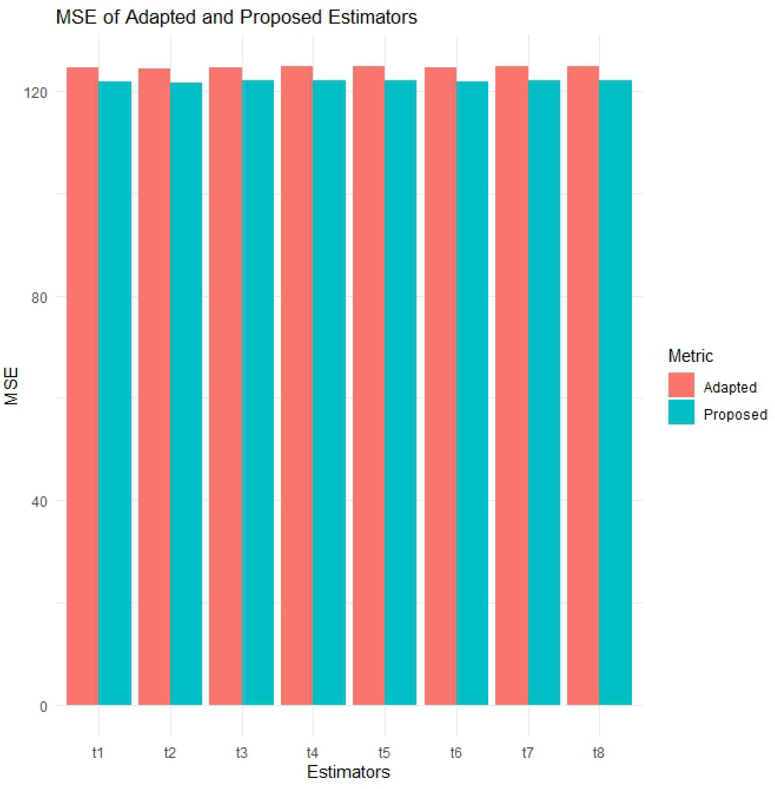
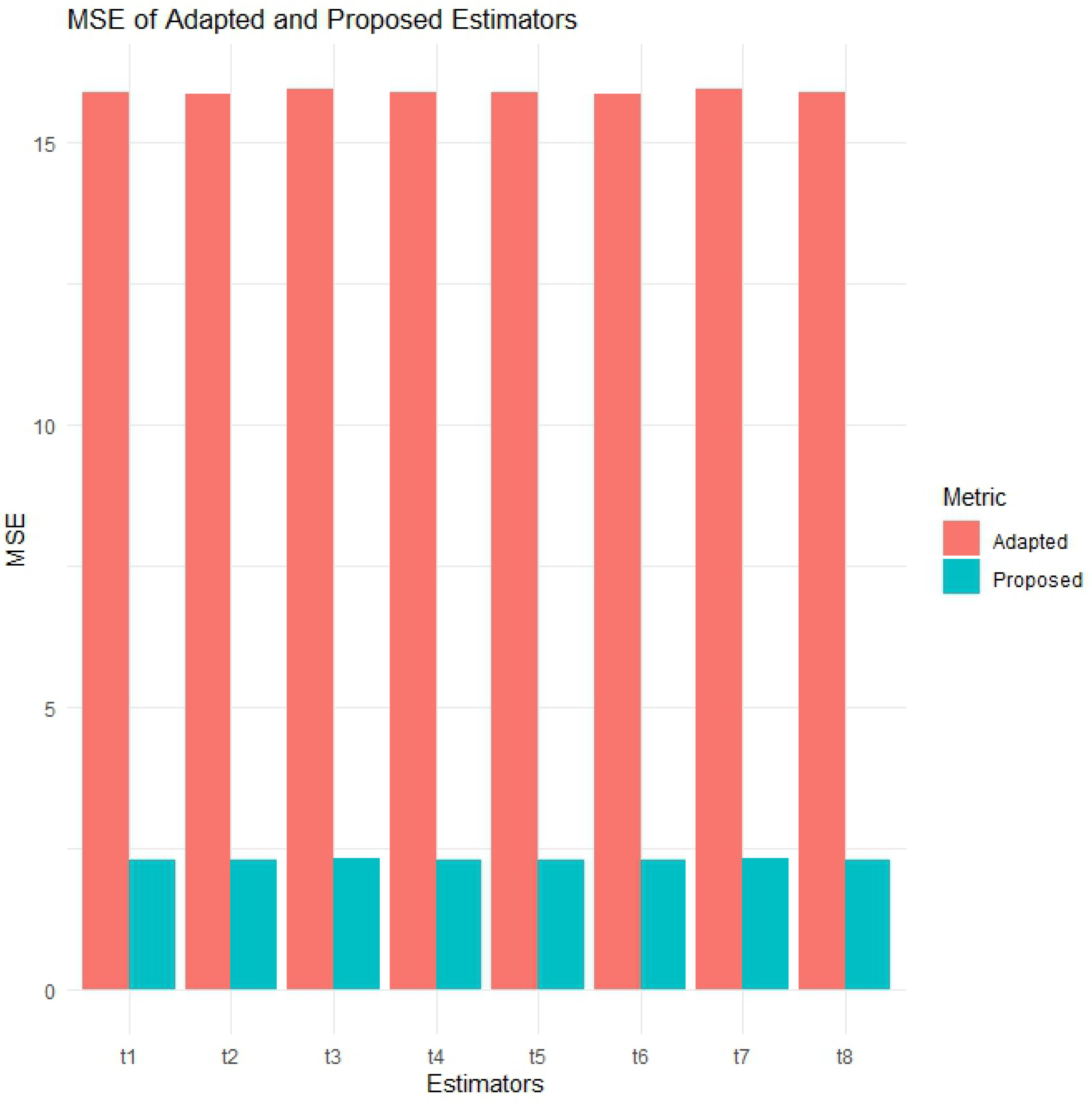
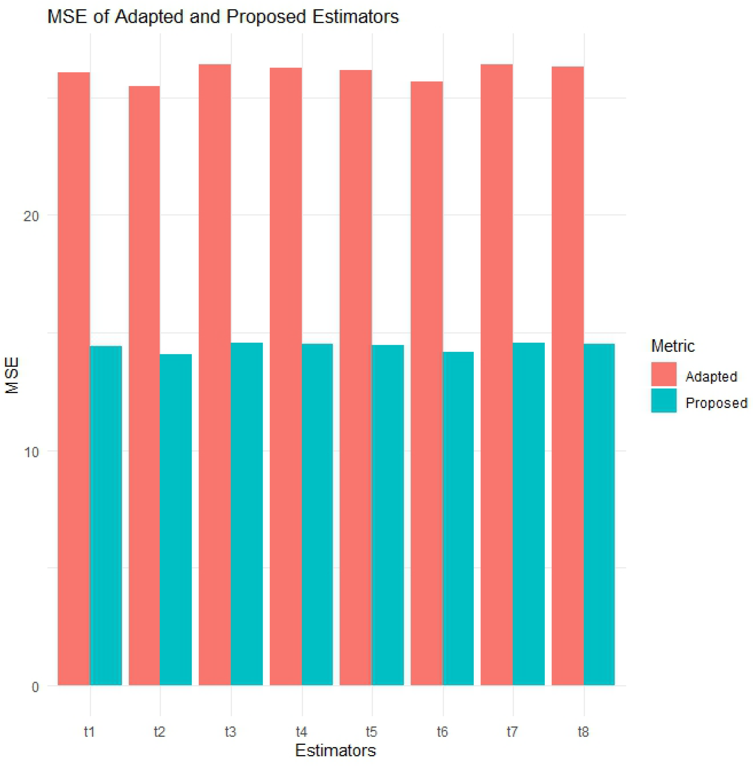
  On all datasets, the ${\widehat{Y}}_{pi}$ (proposed) estimators show smaller MSE values compared to the adapted ones, ${\widehat{Y}}_{G1}$–${\widehat{Y}}_{G8}$. For adapted methods, the results show that MSE values range from 15.85618 for ${\widehat{Y}}_{G2}$ to 15.93169 for ${\widehat{Y}}_{G7}$. On the other hand, ${\widehat{Y}}_{pi}$ approaches reported MSE values ranging from 2.291056 for ${\widehat{Y}}_{p2}$ to 2.307062 for ${\widehat{Y}}_{p7}$. These findings indicate that ${\widehat{Y}}_{pi}$ methods provide very precise results, reducing estimation errors by more than 85%.
• Improved estimation consistency in Education and Wheat datasets:
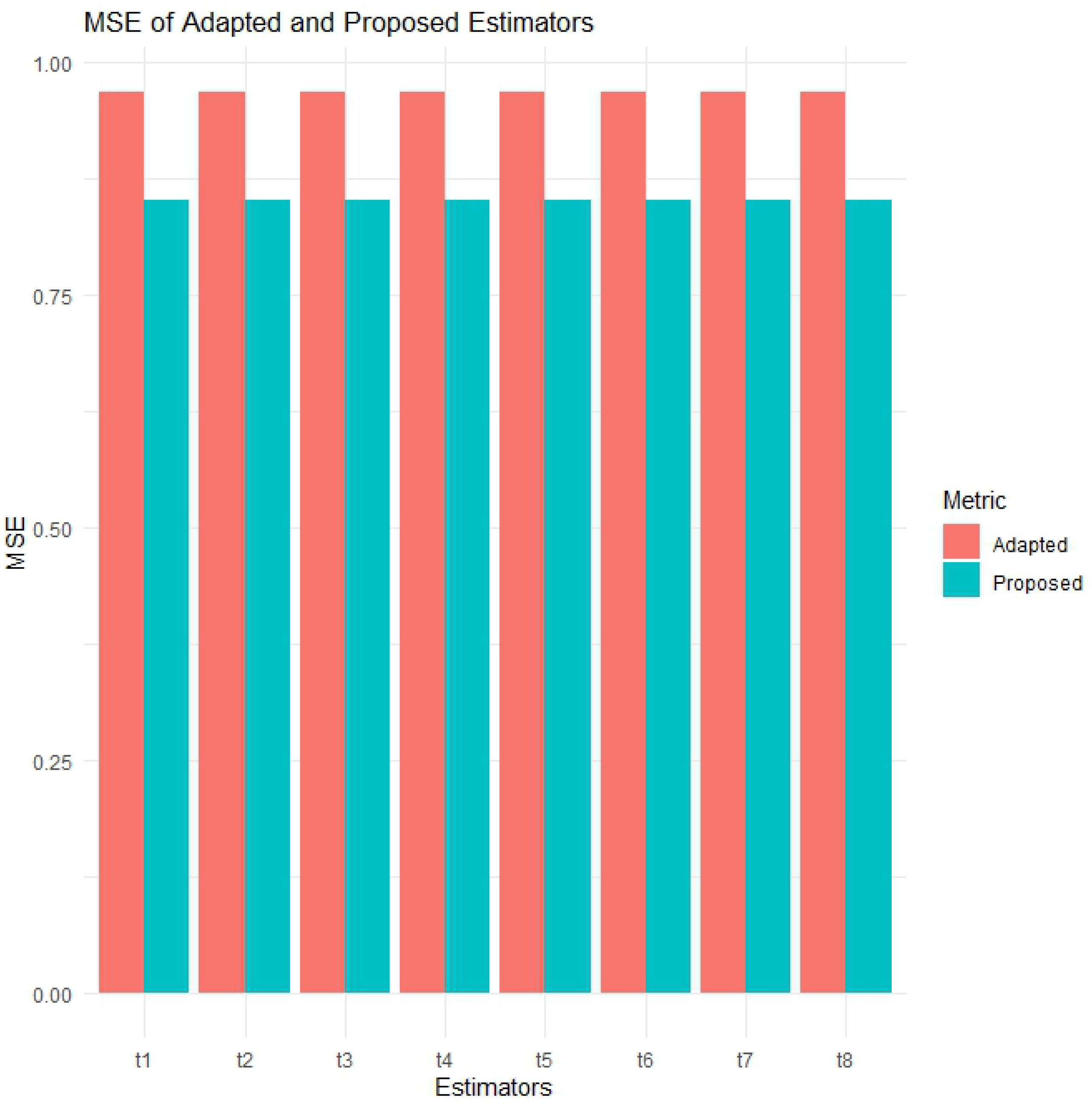
  In the Education dataset, the adapted methods produce MSEs of around 0.9672 (for instance, ${\widehat{Y}}_{G1}$ = 0.9672025), whereas ${\widehat{Y}}_{pi}$ estimators have MSEs of around 0.8513 (for example, ${\widehat{Y}}_{G1}$ = 0.8513346), representing a 12% improvement. The values of the MSE of the Wheat dataset in ${\widehat{Y}}_{G8}$ and ${\widehat{Y}}_{p2}$ are 124.8 and 121.7, respectively, indicating a decrease of about 2.5%. These enhancements, although small, show that the ${\widehat{Y}}_{pi}$ method is more accurate and reliable.
• Low variability and high stability among $\widehat{Y}pi$ estimators: The $\widehat{Y}pi$ methods exhibit an extremely high level of stability in every dataset with little variation. For example, in the Education dataset, the proposed estimators’ MSEs range narrowly from 0.8512927 ($\widehat{Y}p2$) to 0.8513584 ($\widehat{Y}p3$). Similarly, in the Wheat dataset, values stay close between 121.6912 ($\widehat{Y}p2$) and 122.1281 ($\widehat{Y}p8$). Due to this consistency, the ${\widehat{Y}}_{pi}$ estimators are highly dependable for application across multiple datasets.
• Highest efficiency achieved: The $\widehat{Y}pi$ (proposed) estimators consistently yield significantly higher PRE values compared to the adapted estimators $\widehat{Y}G1$ to ${\widehat{Y}}_{G8}$ in all three real-world datasets.

Additionally, the visual representation of the PRE results is provided in Figure 1, Figure 2, Figure 3, Figure 4, Figure 5, Figure 6 and Figure 7. In this visual representation, note that there are eight blocks labeled t1 to t8. Each block t represents a pair of adapted and proposed estimators, such as $\mathrm{t}1ϵ({\widehat{Y}}_{G1},{\widehat{Y}}_{p1})$, $\mathrm{t}2ϵ({\widehat{Y}}_{G2},{\widehat{Y}}_{p2})$, $\mathrm{t}3ϵ({\widehat{Y}}_{G3},{\widehat{Y}}_{p3})$, $\mathrm{t}4ϵ({\widehat{Y}}_{G4},{\widehat{Y}}_{p4})$, $\mathrm{t}5ϵ({\widehat{Y}}_{G5},{\widehat{Y}}_{p5})$, $\mathrm{t}6ϵ({\widehat{Y}}_{G6},{\widehat{Y}}_{p6})$, $\mathrm{t}7ϵ({\widehat{Y}}_{G7},{\widehat{Y}}_{p7})$, and $\mathrm{t}8ϵ({\widehat{Y}}_{G8},{\widehat{Y}}_{p8})$.

Table 7. MSE for real-life datasets.

$\widehat{\mathit{\theta }}$	Education	Wheat	UScereal	Radiation
${\widehat{Y}}_{G1}$	0.9672025	124.5812	15.87095	26.07291
${\widehat{Y}}_{G2}$	0.9671549	124.3671	15.85618	25.45828
${\widehat{Y}}_{G3}$	0.9672294	124.7310	15.92907	26.38176
${\widehat{Y}}_{G4}$	0.9672211	124.7536	15.89097	26.23066
${\widehat{Y}}_{G5}$	0.9672183	124.7505	15.87201	26.15663
${\widehat{Y}}_{G6}$	0.9671926	124.6284	15.85675	25.67837
${\widehat{Y}}_{G7}$	0.9672304	124.8070	15.93169	26.38337
${\widehat{Y}}_{G8}$	0.9672270	124.8137	15.89264	26.27420
${\widehat{Y}}_{p1}$	0.8513346	121.9007	2.294279	14.40656
${\widehat{Y}}_{p2}$	0.8512927	121.6912	2.291056	14.05724
${\widehat{Y}}_{p3}$	0.8513584	122.0473	2.306527	14.57852
${\widehat{Y}}_{p4}$	0.8513511	122.0694	2.298577	14.49470
${\widehat{Y}}_{p5}$	0.8513486	122.0663	2.294510	14.45342
${\widehat{Y}}_{p6}$	0.8513259	121.9469	2.291182	14.18339
${\widehat{Y}}_{p7}$	0.8513592	122.1216	2.307062	14.57941
${\widehat{Y}}_{p8}$	0.8513562	122.1281	2.298932	14.51891

Table 7. MSE for real-life datasets.

$\widehat{\mathit{\theta }}$	Education	Wheat	UScereal	Radiation
${\widehat{Y}}_{G1}$	0.9672025	124.5812	15.87095	26.07291
${\widehat{Y}}_{G2}$	0.9671549	124.3671	15.85618	25.45828
${\widehat{Y}}_{G3}$	0.9672294	124.7310	15.92907	26.38176
${\widehat{Y}}_{G4}$	0.9672211	124.7536	15.89097	26.23066
${\widehat{Y}}_{G5}$	0.9672183	124.7505	15.87201	26.15663
${\widehat{Y}}_{G6}$	0.9671926	124.6284	15.85675	25.67837
${\widehat{Y}}_{G7}$	0.9672304	124.8070	15.93169	26.38337
${\widehat{Y}}_{G8}$	0.9672270	124.8137	15.89264	26.27420
${\widehat{Y}}_{p1}$	0.8513346	121.9007	2.294279	14.40656
${\widehat{Y}}_{p2}$	0.8512927	121.6912	2.291056	14.05724
${\widehat{Y}}_{p3}$	0.8513584	122.0473	2.306527	14.57852
${\widehat{Y}}_{p4}$	0.8513511	122.0694	2.298577	14.49470
${\widehat{Y}}_{p5}$	0.8513486	122.0663	2.294510	14.45342
${\widehat{Y}}_{p6}$	0.8513259	121.9469	2.291182	14.18339
${\widehat{Y}}_{p7}$	0.8513592	122.1216	2.307062	14.57941
${\widehat{Y}}_{p8}$	0.8513562	122.1281	2.298932	14.51891

Table 8. PRE for Education data.

$\widehat{\mathit{\theta }}$	${\widehat{\mathit{Y}}}_{\mathit{p}1}$	${\widehat{\mathit{Y}}}_{\mathit{p}2}$	${\widehat{\mathit{Y}}}_{\mathit{p}3}$	${\widehat{\mathit{Y}}}_{\mathit{p}4}$	${\widehat{\mathit{Y}}}_{\mathit{p}5}$	${\widehat{\mathit{Y}}}_{\mathit{p}6}$	${\widehat{\mathit{Y}}}_{\mathit{p}7}$	${\widehat{\mathit{Y}}}_{\mathit{p}8}$
${\widehat{Y}}_{G1}$	113.6101	113.6045	113.6133	113.6123	113.6120	113.6090	113.6134	113.6130
${\widehat{Y}}_{G2}$	113.6157	113.6101	113.6189	113.6179	113.6176	113.6146	113.6190	113.6186
${\widehat{Y}}_{G3}$	113.6070	113.6014	113.6101	113.6092	113.6088	113.6058	113.6103	113.6099
${\widehat{Y}}_{G4}$	113.6079	113.6024	113.6111	113.6101	113.6098	113.6068	113.6112	113.6108
${\widehat{Y}}_{G5}$	113.6083	113.6027	113.6114	113.6105	113.6101	113.6071	113.6116	113.6112
${\widehat{Y}}_{G6}$	113.6113	113.6057	113.6145	113.6135	113.6132	113.6101	113.6146	113.6142
${\widehat{Y}}_{G7}$	113.6069	113.6013	113.6100	113.6090	113.6087	113.6057	113.6101	113.6097
${\widehat{Y}}_{G8}$	113.6073	113.6017	113.6104	113.6095	113.6091	113.6061	113.6105	113.6101

Table 8. PRE for Education data.

$\widehat{\mathit{\theta }}$	${\widehat{\mathit{Y}}}_{\mathit{p}1}$	${\widehat{\mathit{Y}}}_{\mathit{p}2}$	${\widehat{\mathit{Y}}}_{\mathit{p}3}$	${\widehat{\mathit{Y}}}_{\mathit{p}4}$	${\widehat{\mathit{Y}}}_{\mathit{p}5}$	${\widehat{\mathit{Y}}}_{\mathit{p}6}$	${\widehat{\mathit{Y}}}_{\mathit{p}7}$	${\widehat{\mathit{Y}}}_{\mathit{p}8}$
${\widehat{Y}}_{G1}$	113.6101	113.6045	113.6133	113.6123	113.6120	113.6090	113.6134	113.6130
${\widehat{Y}}_{G2}$	113.6157	113.6101	113.6189	113.6179	113.6176	113.6146	113.6190	113.6186
${\widehat{Y}}_{G3}$	113.6070	113.6014	113.6101	113.6092	113.6088	113.6058	113.6103	113.6099
${\widehat{Y}}_{G4}$	113.6079	113.6024	113.6111	113.6101	113.6098	113.6068	113.6112	113.6108
${\widehat{Y}}_{G5}$	113.6083	113.6027	113.6114	113.6105	113.6101	113.6071	113.6116	113.6112
${\widehat{Y}}_{G6}$	113.6113	113.6057	113.6145	113.6135	113.6132	113.6101	113.6146	113.6142
${\widehat{Y}}_{G7}$	113.6069	113.6013	113.6100	113.6090	113.6087	113.6057	113.6101	113.6097
${\widehat{Y}}_{G8}$	113.6073	113.6017	113.6104	113.6095	113.6091	113.6061	113.6105	113.6101

Table 9. PRE for Wheat data.

$\widehat{\mathit{\theta }}$	${\widehat{\mathit{Y}}}_{\mathit{p}1}$	${\widehat{\mathit{Y}}}_{\mathit{p}2}$	${\widehat{\mathit{Y}}}_{\mathit{p}3}$	${\widehat{\mathit{Y}}}_{\mathit{p}4}$	${\widehat{\mathit{Y}}}_{\mathit{p}5}$	${\widehat{\mathit{Y}}}_{\mathit{p}6}$	${\widehat{\mathit{Y}}}_{\mathit{p}7}$	${\widehat{\mathit{Y}}}_{\mathit{p}8}$
${\widehat{Y}}_{G1}$	102.1989	102.0233	102.3218	102.3404	102.3378	102.2377	102.3842	102.3896
${\widehat{Y}}_{G2}$	102.3749	102.1990	102.4980	102.5165	102.5140	102.4137	102.5604	102.5659
${\widehat{Y}}_{G3}$	102.0762	101.9008	102.1989	102.2174	102.2149	102.1149	102.2612	102.2667
${\widehat{Y}}_{G4}$	102.0577	101.8823	102.1805	102.1989	102.1964	102.0964	102.2427	102.2482
${\widehat{Y}}_{G5}$	102.0603	101.8849	102.1830	102.2015	102.1989	102.0989	102.2453	102.2507
${\widehat{Y}}_{G6}$	102.1603	101.9847	102.2831	102.3016	102.2990	102.1989	102.3454	102.3509
${\widehat{Y}}_{G7}$	102.0140	101.8387	102.1367	102.1552	102.1526	102.0527	102.1989	102.2044
${\widehat{Y}}_{G8}$	102.0086	101.8333	102.1313	102.1497	102.1472	102.0472	102.1935	102.1989

Table 9. PRE for Wheat data.

$\widehat{\mathit{\theta }}$	${\widehat{\mathit{Y}}}_{\mathit{p}1}$	${\widehat{\mathit{Y}}}_{\mathit{p}2}$	${\widehat{\mathit{Y}}}_{\mathit{p}3}$	${\widehat{\mathit{Y}}}_{\mathit{p}4}$	${\widehat{\mathit{Y}}}_{\mathit{p}5}$	${\widehat{\mathit{Y}}}_{\mathit{p}6}$	${\widehat{\mathit{Y}}}_{\mathit{p}7}$	${\widehat{\mathit{Y}}}_{\mathit{p}8}$
${\widehat{Y}}_{G1}$	102.1989	102.0233	102.3218	102.3404	102.3378	102.2377	102.3842	102.3896
${\widehat{Y}}_{G2}$	102.3749	102.1990	102.4980	102.5165	102.5140	102.4137	102.5604	102.5659
${\widehat{Y}}_{G3}$	102.0762	101.9008	102.1989	102.2174	102.2149	102.1149	102.2612	102.2667
${\widehat{Y}}_{G4}$	102.0577	101.8823	102.1805	102.1989	102.1964	102.0964	102.2427	102.2482
${\widehat{Y}}_{G5}$	102.0603	101.8849	102.1830	102.2015	102.1989	102.0989	102.2453	102.2507
${\widehat{Y}}_{G6}$	102.1603	101.9847	102.2831	102.3016	102.2990	102.1989	102.3454	102.3509
${\widehat{Y}}_{G7}$	102.0140	101.8387	102.1367	102.1552	102.1526	102.0527	102.1989	102.2044
${\widehat{Y}}_{G8}$	102.0086	101.8333	102.1313	102.1497	102.1472	102.0472	102.1935	102.1989

Table 10. PRE for UScereal data.

$\widehat{\mathit{\theta }}$	${\widehat{\mathit{Y}}}_{\mathit{p}1}$	${\widehat{\mathit{Y}}}_{\mathit{p}2}$	${\widehat{\mathit{Y}}}_{\mathit{p}3}$	${\widehat{\mathit{Y}}}_{\mathit{p}4}$	${\widehat{\mathit{Y}}}_{\mathit{p}5}$	${\widehat{\mathit{Y}}}_{\mathit{p}6}$	${\widehat{\mathit{Y}}}_{\mathit{p}7}$	${\widehat{\mathit{Y}}}_{\mathit{p}8}$
${\widehat{Y}}_{G1}$	691.7618	691.1182	694.2953	692.6344	691.8083	691.1432	694.4095	692.7072
${\widehat{Y}}_{G2}$	692.7350	692.0905	695.2721	693.6088	692.7815	692.1155	695.3864	693.6817
${\widehat{Y}}_{G3}$	688.0886	687.4484	690.6087	688.9565	688.1348	687.4732	690.7222	689.0290
${\widehat{Y}}_{G4}$	690.4683	689.8259	692.9971	691.3393	690.5147	689.8509	693.1111	691.4120
${\widehat{Y}}_{G5}$	691.6922	691.0487	694.2255	692.5647	691.7386	691.0736	694.3396	692.6375
${\widehat{Y}}_{G6}$	692.6969	692.0525	695.2339	693.5707	692.7435	692.0775	695.3482	693.6436
${\widehat{Y}}_{G7}$	687.9291	687.2890	690.4486	688.7968	687.9753	687.3139	690.5621	688.8692
${\widehat{Y}}_{G8}$	690.3617	689.7194	692.8901	691.2325	690.4080	689.7443	693.0040	691.3052

Table 10. PRE for UScereal data.

$\widehat{\mathit{\theta }}$	${\widehat{\mathit{Y}}}_{\mathit{p}1}$	${\widehat{\mathit{Y}}}_{\mathit{p}2}$	${\widehat{\mathit{Y}}}_{\mathit{p}3}$	${\widehat{\mathit{Y}}}_{\mathit{p}4}$	${\widehat{\mathit{Y}}}_{\mathit{p}5}$	${\widehat{\mathit{Y}}}_{\mathit{p}6}$	${\widehat{\mathit{Y}}}_{\mathit{p}7}$	${\widehat{\mathit{Y}}}_{\mathit{p}8}$
${\widehat{Y}}_{G1}$	691.7618	691.1182	694.2953	692.6344	691.8083	691.1432	694.4095	692.7072
${\widehat{Y}}_{G2}$	692.7350	692.0905	695.2721	693.6088	692.7815	692.1155	695.3864	693.6817
${\widehat{Y}}_{G3}$	688.0886	687.4484	690.6087	688.9565	688.1348	687.4732	690.7222	689.0290
${\widehat{Y}}_{G4}$	690.4683	689.8259	692.9971	691.3393	690.5147	689.8509	693.1111	691.4120
${\widehat{Y}}_{G5}$	691.6922	691.0487	694.2255	692.5647	691.7386	691.0736	694.3396	692.6375
${\widehat{Y}}_{G6}$	692.6969	692.0525	695.2339	693.5707	692.7435	692.0775	695.3482	693.6436
${\widehat{Y}}_{G7}$	687.9291	687.2890	690.4486	688.7968	687.9753	687.3139	690.5621	688.8692
${\widehat{Y}}_{G8}$	690.3617	689.7194	692.8901	691.2325	690.4080	689.7443	693.0040	691.3052

Table 11. PRE for Meteorological Solar Radiation data.

$\widehat{\mathit{\theta }}$	${\widehat{\mathit{Y}}}_{\mathit{p}1}$	${\widehat{\mathit{Y}}}_{\mathit{p}2}$	${\widehat{\mathit{Y}}}_{\mathit{p}3}$	${\widehat{\mathit{Y}}}_{\mathit{p}4}$	${\widehat{\mathit{Y}}}_{\mathit{p}5}$	${\widehat{\mathit{Y}}}_{\mathit{p}6}$	${\widehat{\mathit{Y}}}_{\mathit{p}7}$	${\widehat{\mathit{Y}}}_{\mathit{p}8}$
${\widehat{Y}}_{G1}$	180.9794	176.7131	183.1232	182.0744	181.5605	178.2408	183.1344	182.3766
${\widehat{Y}}_{G2}$	185.4767	181.1043	187.6738	186.5989	186.0723	182.6700	187.6853	186.9086
${\widehat{Y}}_{G3}$	178.8448	174.6287	180.9633	179.9268	179.4190	176.1384	180.9743	180.2255
${\widehat{Y}}_{G4}$	179.8790	175.6386	182.0097	180.9673	180.4566	177.1570	182.0209	181.2677
${\widehat{Y}}_{G5}$	180.3927	176.1402	182.5296	181.4842	180.9720	177.6630	182.5407	181.7854
${\widehat{Y}}_{G6}$	183.8271	179.4936	186.0046	184.9393	184.4174	181.0454	186.0160	185.2463
${\widehat{Y}}_{G7}$	178.8338	174.6181	180.9522	179.9158	179.4081	176.1277	180.9633	180.2145
${\widehat{Y}}_{G8}$	179.5790	175.3456	181.7062	180.6655	180.1556	176.8615	181.7173	180.9654

Table 11. PRE for Meteorological Solar Radiation data.

$\widehat{\mathit{\theta }}$	${\widehat{\mathit{Y}}}_{\mathit{p}1}$	${\widehat{\mathit{Y}}}_{\mathit{p}2}$	${\widehat{\mathit{Y}}}_{\mathit{p}3}$	${\widehat{\mathit{Y}}}_{\mathit{p}4}$	${\widehat{\mathit{Y}}}_{\mathit{p}5}$	${\widehat{\mathit{Y}}}_{\mathit{p}6}$	${\widehat{\mathit{Y}}}_{\mathit{p}7}$	${\widehat{\mathit{Y}}}_{\mathit{p}8}$
${\widehat{Y}}_{G1}$	180.9794	176.7131	183.1232	182.0744	181.5605	178.2408	183.1344	182.3766
${\widehat{Y}}_{G2}$	185.4767	181.1043	187.6738	186.5989	186.0723	182.6700	187.6853	186.9086
${\widehat{Y}}_{G3}$	178.8448	174.6287	180.9633	179.9268	179.4190	176.1384	180.9743	180.2255
${\widehat{Y}}_{G4}$	179.8790	175.6386	182.0097	180.9673	180.4566	177.1570	182.0209	181.2677
${\widehat{Y}}_{G5}$	180.3927	176.1402	182.5296	181.4842	180.9720	177.6630	182.5407	181.7854
${\widehat{Y}}_{G6}$	183.8271	179.4936	186.0046	184.9393	184.4174	181.0454	186.0160	185.2463
${\widehat{Y}}_{G7}$	178.8338	174.6181	180.9522	179.9158	179.4081	176.1277	180.9633	180.2145
${\widehat{Y}}_{G8}$	179.5790	175.3456	181.7062	180.6655	180.1556	176.8615	181.7173	180.9654

The MSE plots for the simulations and Education, Wheat, UScereal, and Meteorological Solar Radiation datasets provide a visual confirmation of the dominant performance of ${\widehat{Y}}_{p1}-{\widehat{Y}}_{p8}$.

5. Conclusions

In this study, a unified class of mean estimation methods was established employing the median as the pre-specified value of the target variable along with the raw measures of the dispersion of auxiliary variables, including the interquartile range, semi-interquartile range, mid-range, and interdecile range. The methodology offers a new addition to survey sampling, where traditional methods usually use the average of auxiliary variables and underutilize the median, even though this is a more robust statistic against distributional aberrations. To fill this gap, two broad classes of estimators were suggested: adapted exponential-type (AET) estimators and generalized exponential-type (GET) estimators, each of which aims to use the joint power of the known median and auxiliary information. Theoretical derivations showed that under ideal circumstances, the GET estimators exhibit lower MSE, and the results were consistently confirmed by simulation studies using Kumaraswamy–Gamma populations. Moreover, the empirical results based on datasets from the education, agriculture, and nutrition fields, as well as a real-world meteorological test with solar radiation data of the HI-SEAS(HS) weather station, indicate that the proposed estimators outperform the current methods by a significant margin. These findings underscore the applicability of the proposed framework in practice, indicating that it may be applied not only in conventional areas of surveys but also in the development of environmental and energy-associated research in which solar radiation is a central figure. Furthermore, the suggested framework can be expanded to complex sampling schemes like stratified, two-stage, and double sampling and to models involving non-response and measurement error in future research.

References

- Alomair, A.M.; Shahzad, U. Tweedie-Poisson regression-based mean estimation of dose equivalence rates using gamma count auxiliary information. J. Radiat. Res. Appl. Sci. 2025, 18, 101929. [Google Scholar] [CrossRef]
- Chutiman, N.; Nathomthong, A.; Wichitchan, S.; Guayjarernpanishk, P. Improved Estimator Using Auxiliary Information in Adaptive Cluster Sampling with Networks Selected Without Replacement. Symmetry 2025, 17, 375. [Google Scholar] [CrossRef]
- Alomair, A.M.; Shahzad, U. Optimizing mean estimators with calibrated minimum covariance determinant in median ranked set sampling. Symmetry 2023, 15, 1581. [Google Scholar] [CrossRef]
- Koc, T.; Koc, H. A new class of quantile regression ratio-type estimators for finite population mean in stratified random sampling. Axioms 2023, 12, 713. [Google Scholar] [CrossRef]
- Kuk, Y.A.; Mak, K.T. Median estimation in the presence of auxiliary information. J. R. Stat. Soc. Ser. (Methodol.) 1989, 51, 261–269. [Google Scholar] [CrossRef]
- Subramani, J. A new modified ratio estimator for estimation of population mean when median of the auxiliary variable is known. Pak. J. Stat. Oper. Res. 2013, 9, 137–145. [Google Scholar] [CrossRef]
- Subramani, J. A new median based ratio estimator for estimation of the finite population mean. Stat. Transit. New Ser. 2016, 17, 591–604. [Google Scholar] [CrossRef]
- Lamichhane, R.; Singh, S.; Diawara, N. Improved estimation of population mean using known median of auxiliary variable. Commun. Stat. Simul. Comput. 2017, 46, 2821–2828. [Google Scholar] [CrossRef]
- Irfan, M.; Javed, M.; Abid, M.; Lin, Z. Improved ratio type estimators of population mean based on median of a study variable and an auxiliary variable. Hacet. J. Math. Stat. 2018, 47, 659–673. [Google Scholar] [CrossRef]
- Yusuf, A.Y.; Audu, A.; Yunusa, M.A. Power median-based estimators of finite population mean. Fudma J. Sci. 2024, 8, 296–300. [Google Scholar] [CrossRef]
- Shahzad, U.; Al-Noor, N.H.; Hanif, M.; Sajjad, I. An exponential family of median based estimators for mean estimation with simple random sampling scheme. Commun. Stat. Theory Methods 2021, 50, 4890–4899. [Google Scholar] [CrossRef]
- Saini, M.; Jitendrakumar, B.R.; Kumar, A. Improved ratio estimator under simple and stratified random sampling. Life Cycle Reliab. Saf. Eng. 2024, 13, 181–187. [Google Scholar] [CrossRef]
- Abdullahi, U.K.; Ugwuowo, F.I. On efficient median-based linear regression estimator for population mean. Commun. Stat. Theory Methods 2022, 51, 5012–5024. [Google Scholar] [CrossRef]
- Singh, R.; Tiwari, S.N. Improved Estimator for Population Mean Utilizing Known Medians of Two Auxiliary Variables under Neutrosophic Framework. Neutrosophic Syst. Appl. 2025, 25, 38–52. [Google Scholar] [CrossRef]
- Kurbah, R.E.; Khongji, P.; Hynniewta, B.C. Efficient rank set sampling estimators of mean using median under double sampling with two auxiliary variables. Adv. Appl. Stat. 2024, 91, 943–968. [Google Scholar] [CrossRef]
- Soni, S.S.; Pandey, H. Generalized estimator of population variance utilizing auxiliary information in simple random sampling scheme. J. Probab. Stat. Sci. 2023, 21, 23–33. [Google Scholar] [CrossRef]
- Naz, F.; Nawaz, T.; Pang, T.; Abid, M. Use of Nonconventional Dispersion Measures to Improve the Efficiency of Ratio-Type Estimators of Variance in the Presence of Outliers. Symmetry 2020, 12, 16. [Google Scholar] [CrossRef]
- Cetin, A.E.; Koyuncu, N. Calibration estimator of population mean in stratified extreme ranked set sampling with simulation study. Filomat 2024, 38, 599–608. [Google Scholar] [CrossRef]
- Cetin, A.E.; Koyuncu, N. Robust regression type estimators for body mass index under extreme ranked set and quartile ranked set sampling. Commun. Fac. Sci. Univ. Ank. Ser. Math. Stat. 2024, 73, 336–348. [Google Scholar]
- Cetin, A.E.; Koyuncu, N. New robust class of estimators for population mean under different sampling designs. J. Comput. Appl. Math. 2024, 441, 115669. [Google Scholar] [CrossRef]
- Zaman, T.; Bulut, H. A simulation study: Robust ratio double sampling estimator of finite population mean in the presence of outliers. Sci. Iran. 2024, 31, 1330–1341. [Google Scholar] [CrossRef]
- Zaman, T.; Shazad, U.; Yadav, V.K. An efficient Hartley–Ross type estimators of nonsensitive and sensitive variables using robust regression methods in sample surveys. J. Comput. Appl. Math. 2024, 440, 115645. [Google Scholar] [CrossRef]
- Rashedi, K.A.; Abdulrahman, A.T.; Alshammari, T.S.; Alshammari, K.M.; Shahzad, U.; Shabbir, J.; Ahmad, I. Robust Särndal-Type Mean Estimators with Re-Descending Coefficients. Axioms 2025, 14, 261. [Google Scholar] [CrossRef]
- Mishra, R.; Singh, R.; Adichwal, N.K. A novel ratio cum product type exponential class of estimators of finite population mean in Adaptive cluster Sampling. Braz. J. Biom. 2025, 43, e43745. [Google Scholar] [CrossRef]
- Daraz, U.; Wu, J.; Albalawi, O. Double exponential ratio estimator of a finite population variance under extreme values in simple random sampling. Mathematics 2024, 12, 1737. [Google Scholar] [CrossRef]
- Alharbi, R.; Mustafa, M.S.; Al Mutairi, A.; Hussein, M.; Yusuf, M.; Elshenawy, A.; Nassr, S.G. Enhancing mean estimators in median ranked set sampling with dual auxiliary information. Heliyon 2023, 9, e21427. [Google Scholar] [CrossRef] [PubMed]
- De Pascoa, M.A.; Ortega, E.M.; Cordeiro, G.M. The Kumaraswamy generalized gamma distribution with application in survival analysis. Stat. Methodol. 2011, 8, 411–433. [Google Scholar] [CrossRef]
- Arshad, R.M.I.; Tahir, M.H.; Chesneau, C.; Jamal, F. The Gamma Kumaraswamy-G family of distributions: Theory, inference and applications. Stat. Transit. New Ser. 2020, 21, 17–40. [Google Scholar] [CrossRef]
- Chatterjee, S.; Hadi, S.A. Regression Analysis by Example; John Wiley and Sons: Hoboken, NJ, USA, 2015. [Google Scholar]
- Maechler, M.; Rousseeuw, P.; Croux, C.; Todorov, V.; Ruckstuhl, A.; Salibian-Barrera, M.; di Palma, M.A. Robustbase: Basic Robust Statistics R Package Version 0.92-7. 2016. Available online: http://CRAN.R-project.org/package=robustbase (accessed on 5 February 2025).
- Sukhatme, P.V.; Sukhatme, B.V. Sampling Theory of Surveys with Application; Iowa Statistical University Press: Iowa City, IA, USA, 1970. [Google Scholar]
- Venables, W.N.; Ripley, B.D. Modern Applied Statistics with S-PLUS, 3rd ed.; Springer: Berlin/Heidelberg, Germany, 1999. [Google Scholar]