1. Introduction
The level of food quality is not only related to public health, economic development, and social stability but also to national governance capacity and government credibility. It has long been a core issue in public governance. With the continuous development of the economy and society and the improvement of residents’ income, the public demand for food quality and safety is increasing, which brings new challenges to food safety management. People’s pursuit of a better life is driving the upgrading of the consumption structure, which has shifted from “being full” to “eating well and eating healthily”. Green food, with its low pesticide and veterinary drug residues and high nutritional safety, has become a key support point for improving social welfare. On the one hand, consuming green food can significantly reduce the risk of chronic diseases and ease the burden of public health systems; on the other hand, the green transition is pushing government governance goals from “safety production” to “quality improvement”.
Differential game theory originated from air combat research. During World War II, due to military strategic needs, Dr. Isaacs from the RAND Corporation in the United States led the study of pursuit–evasion problems, where both sides could make free strategic decisions. This combined optimal control with game theory. The publication of Isaacs’ monograph Differential Games [
1] formally marked the birth of differential game theory, which describes the interaction of strategies between players through differential equations of states. Together with Bellman’s Dynamic Programming [
2] and Pontryagin et al.’s The Mathematical Theory of Optimal Processes [
3], it laid the theoretical foundation for differential games. Starr and Ho [
4] developed a non-zero-sum differential game model, extending the theory to multi-player non-zero-sum cases, and explained the differences between zero-sum and non-zero-sum games. Fershtman [
5] investigated structural issues in differential games. In a separate context, Basar and Zhu [
6] pointed out that the price of anarchy has been widely used in static games to quantify the efficiency loss resulting from non-cooperative behavior. They also introduced the price of information to characterize differences in game performance under varying information structures and proposed the price of cooperation to measure the extent of gain or loss experienced by participants due to altruistic behaviors. They introduced the concept of anarchy cost in static games to measure efficiency loss due to non-cooperative behavior and further proposed information costs and cooperation costs to quantify performance under different information structures and altruistic behaviors. In 2016, Google’s AlphaGo combined dynamic games and reinforcement learning to defeat a human world champion in Go for the first time. Buckdahn et al. [
7] studied stochastic differential games with state constraints using backward stochastic differential equations, while Platzer [
8] enhanced the logic of differential games with hybrid game dynamics, introducing invariants and variants for inductive proofs of game properties.
Differential game theory has been widely applied in the field of supply chain management due to its ability to precisely capture dynamic strategic interactions, and substantial research outcomes have been achieved in this area. Cao et al. [
9] built a game model with a manufacturer as leader and a retailer as follower, in which the retailer undertakes promotional efforts. Their study showed that regardless of product quality, retailers usually still prefer to promote even if manufacturers do not share the promotion cost. Cheng et al. [
10] applied differential game theory to investigate corporate social responsibility in scenarios involving decentralized, centralized, and joint decision-making. Zu et al. [
11] addressed the growing concerns from various societal stakeholders—including consumers, governments, and firms—regarding low-carbon production. Using a Stackelberg differential game framework, they investigated a two-echelon supply chain consisting of a single manufacturer and a single supplier in three progressive environmental regulation scenarios. Zeng et al. [
12] analyzed cooperation strategies among governments, suppliers, and manufacturers in green supply chains in non-cooperative, government-led, and collaborative contexts. Yang et al. [
13] explored low-carbon production using uncertain differential games, focusing on dynamic equilibrium strategies, emission reduction, and profit trajectories in scenarios involving cooperation and non-cooperation. Jena et al. [
14] introduced cost-sharing mechanisms for advertising into a closed-loop supply chain with uncertain demand and returns and found that such contracts improve overall profit. Chakraborty et al. [
15] examined the effect of cost-sharing contracts on product quality improvement strategies in competitive settings, concluding that they enhance both quality and profitability. He et al. [
16] analyzed cooperative advertising strategies in a two-generation product supply chain, showing that two-way cost-sharing contracts with transfer payments can achieve coordination. Savaskan et al. [
17] studied optimal design of recycling channels and argued that when the manufacturer is the channel leader, retailer-led recycling is optimal. Choi et al. [
18] investigated the effect of different power structures on closed-loop supply chains and found that retailer-led structures yield the highest profits. Chen et al. [
19] built a differential game model for suppliers and retailers in different decision-making contexts, showing Pareto improvements when shifting from decentralized to incentive-based decisions. Sun and Wang [
20] considered the role of food safety incidents and traceability in procurement, finding that traceability improves food safety levels. He et al. [
21] developed a three-tier supply chain model that included suppliers, manufacturers, and retailers and studied profit differences under different government subsidy coefficients. Parisa et al. [
22] analyzed retailer high-end private brand strategies based on leader–follower differential games, showing that introducing high-end private brands alongside national brands can improve retailer profits and that coordination contracts such as two-part tariff contracts can achieve perfect coordination. Zhou et al. [
23] constructed a differential game model with delay effects to analyze optimal traceability levels in food supply chains, concluding that delay time is positively correlated with traceability effort. Zhu et al. [
24] emphasized the role of reference price effects in improving traceability efforts, where core enterprises need to incentivize members to raise traceability levels and share product information. Wang and Zhao [
25] studied the interaction between consumer food safety awareness and cold chain investment, suggesting that governments should encourage consumer awareness to stimulate cold chain investment and ensure food safety.
Existing studies have made valuable contributions to the analysis of continuous-time strategic interactions, particularly in supply chain management, where differential game approaches have been employed to model the strategic choices of supply chain members in dynamic processes. These works provide a theoretical foundation for analyzing the optimal strategies of players in continuously evolving environments and reveal how dynamic feedback mechanisms influence strategy adjustments and policy outcomes. However, there remains limited literature on the optimal strategy selection for food quality improvement under government coordination. Specifically, insufficient attention has been paid to the continuous-time strategic interaction between the government and enterprises in enhancing food quality, and few studies have incorporated the dynamic impact of shadow prices under resource constraints. The influence of government dynamic coordination mechanisms on optimal policy pathways still warrants in-depth investigation.
To address this gap, this study adopts a differential game framework to examine optimal control for food quality improvement from a continuous-time perspective. We develop a differential game model between food producers and government regulators under green technology investment, exploring their optimal strategic paths. The analysis focuses on the enterprise’s optimal pricing and production decisions, as well as the government’s optimal taxation and quality investment policies, aligned with food quality objectives. Furthermore, under resource constraints, this study investigates the evolution of shadow prices. The results demonstrate that varying shadow prices significantly affect the government’s optimal tax policy and quality investment levels, as well as the enterprise’s optimal pricing, output, and green technology investment. A numerical simulation validates the influence of key parameters such as shadow prices and price elasticity coefficients on the system’s evolutionary trajectory, offering theoretical and practical support for the green transition of the food industry.
2. Assumptions and Model Construction
2.1. Notation and Assumptions
The notations used in this study are explained in
Table 1.
We make the following assumptions for the established Stackelberg differential game model:
Assumption 1.
The local government aims to maximize social welfare, while a food producer aims to maximize profit.
Assumption 2.
There are only two non-cooperative firms producing homogeneous products in the market, and both firms have limited production capacity.
Assumption 3.
Firms improve food quality and reduce the probability of food safety incidents by investing in green technology. A larger value of indicates a higher level of green technology, while a smaller value of indicates a lower level. The dynamic evolution of green technology follows the differential equation below:
Here, represents the efficiency of converting financial investment into technology, and denotes the depreciation rate of technology. The growth rate of a firm’s green technology level is positively influenced by its R&D investment, while also being negatively affected by the higher level of green technology itself. Increasing R&D investment can accelerate the improvement of green technology, but the higher the existing technology level, the more difficult it becomes to achieve further improvements.
Assumption 4.
The firm’s unit food quality improvement level is linearly related to its green technology level, where b represents the coefficient measuring the impact of technology improvement on food quality. The relationship is expressed by the following equation:
Assumption 5.
The potential demand in the food market is assumed to remain constant.
2.2. Stackelberg Differential Game Model
According to Fibich et al. [
26], the food output of the firm at time
is given by
Here,
represents the potential market demand,
denotes the price sensitivity of demand,
measures consumers’ sensitivity to the difference between the reference price and the selling price, and
is the price difference between the food-producing firm and its competitor. The reference price can be defined as an internal price that consumers compare with observed prices, which is constructed based on consumers’ personal shopping experiences and exposure to price information. The coefficient
represents the sensitivity of food quality improvement to technological investment. In this study, the competitor’s price
is taken as the reference price. According to Fibich et al. [
26], the change in the reference price is given by the following equation:
Here, represents the memory effect of the price difference.
The profit of the firm at time
is given by the following equation. It calculates the enterprise’s profit by subtracting three costs (production cost, green technology investment cost, and tax) from its revenue:
Here,
denotes the revenue obtained by the firm from selling food at time
;
represents the cost of producing
units of product, with
as the production cost coefficient;
indicates the total cost incurred by the firm to improve green technology by investing
, with
as the technology conversion cost coefficient; and
is the tax paid by the firm (following the study by Saltari and Travaglini [
27]).
The food quality level within the local government’s jurisdiction satisfies the following dynamic equation. It shows that the local food quality level
is promoted by two factors: the enterprise’s green technology investment
and the government’s quality investment
while it decreases due to natural decay
.
Here,
represents the effect of the firm’s investment in improving green technology on the food quality level,
denotes the impact of the local government’s investment in food quality improvement and
is the natural decay rate of food quality (see Liu et al. [
28]).
Improving food quality not only significantly enhances consumers’ health but also generates social welfare benefits. Let the social welfare at time
be expressed as follows:
Here,
denotes the social welfare at the initial time, and
represents the coefficient of social welfare contributed by the food quality level within the local government’s jurisdiction. The revenue of the local government at time
is given by the following equation:
Here, denotes the tax paid by the firm; represents the cost to the local government when the food quality improvement investment level is ; and is the cost coefficient of the local government’s food quality improvement investment.
The objective function of the firm is given by the following equation:
Here, denotes the reward–penalty coefficient, and represents the reward–penalty term set by the local government for the firm. If , it indicates that the firm’s food quality level exceeds the standard set by the local government, and the government provides a reward; otherwise, the government imposes a penalty. represents the firm’s discount rate.
The objective function of the government is given by the following equation:
Here, denotes the reward–penalty coefficient, and represents the reward–penalty term set by the central government for the local government. If , it indicates that the food quality level within the local government’s jurisdiction exceeds the standard set by the central government, and the central government provides a reward; otherwise, the central government imposes a penalty. represents the discount rate of the local government.
Based on the above, a non-cooperative differential game model between the local government and the firm can be established as follows:
Here, .
In the constructed Stackelberg differential game model, the food-producing firm aims to choose its optimal product price and investment in green technology to maximize its own profit, while the local government seeks to select the optimal unit product tax and the optimal food quality improvement investment to maximize social welfare.
3. Solution of the Stackelberg Differential Game Model
In this section, Pontryagin’s maximum principle is applied to solve the constructed Stackelberg differential game model.
Theorem 1.
The firm’s optimal product price and the optimal investment
in green technology are given by the following equations:
where the first equation calculates the enterprise’s optimal pricing by considering market demand, competitor prices, taxes, and reference price effects; the second equation determines the optimal green technology investment based on the shadow prices of technology and quality.
Proof: The Hamiltonian function of the firm is constructed as follows:
Here, are the firm’s shadow prices, where represents the effect of the reference price on the firm’s profit, represents the effect of the firm’s green technology level on its profit, and represents the effect of the food quality level within the local government’s jurisdiction on the firm’s profit.
According to Pontryagin’s maximum principle, by solving the optimization problem of the Hamiltonian function, the values
and
that maximize the firm’s profit are obtained, as given by the following equations:
From the above equations, the necessary conditions for the function to attain an extremum can be obtained.
The co-state (adjoint) equations are given as follows:
From Equations (15) and (16), the firm’s optimal product price
and the optimal investment
in improving green technology can be obtained as follows:
The proof is complete. □
Theorem 2.
The local government’s optimal unit product tax
and the optimal food quality improvement investment are given by the following equations:
where the first equation sets the optimal tax to balance enterprise costs and market demand; the second equation determines the government’s quality investment based on the shadow price of social welfare.
Proof: The Hamiltonian function of the government is constructed as follows:
From the above equations, the necessary conditions for the function to attain an extremum can be derived.
The co-state (adjoint) equations are given by the following formulas:
By substituting Equations (20) and (21) into the relevant expressions, the optimal unit product tax
and the optimal food quality improvement investment
can be obtained as follows:
The proof is complete. □
Corollary 1. The optimal output of the food-producing firm is given by the following equation:
Corollary 2.
The effect of shadow prices on the firm’s optimal output is given by the following equation:
From Equation (24), it can be seen that an increase in will lead to a decrease in the firm’s optimal food output . This is because an increase in causes the firm’s optimal product price to rise. Under the assumption of constant potential market demand, a higher product price reduces consumers’ willingness to pay, leading the firm to decrease its output. Equation (18) also indicates that are not related to the firm’s optimal food output .
Corollary 3.
The effects of shadow prices on the government’s optimal unit product tax and the optimal food quality improvement level are given as follows:
From Equation (25), it can be seen that an increase in will lead to a decrease in the government’s optimal unit product tax . This is because an increase in reduces the firm’s optimal output , causing the firm to place greater emphasis on food quality. To encourage firms to improve food quality, the government will lower the unit product tax . Additionally, Equation (25) indicates that are not related to the government’s optimal unit product tax . From Equation (26), it can be seen that are not related to the government’s optimal food quality improvement investment . Moreover, an increase in leads to an increase in the government’s optimal food quality improvement investment . This is because a higher indicates that improvements in food quality have a more significant positive impact on social welfare. To enhance social welfare, the government chooses to increase the level of investment in food quality improvement .
Corollary 4.
The effects of shadow prices on the firm’s optimal product price and the optimal investment in improving green technology are given as follows:
From Equation (27), it can be seen that an increase in will lead to a rise in the firm’s optimal product price . This is because an increase in causes the firm to reduce output; therefore, to obtain higher profits, the firm chooses to raise its product price. It can also be seen that are not related to the firm’s optimal product price . From Equation (28), it can be seen that are not related to the firm’s optimal investment in improving production technology. Moreover, an increase in leads to an increase in the firm’s optimal investment in green technology. This is because represents the impact of the firm’s green technology level on its profit, and an increase in indicates that the firm’s production technology has a more significant effect on profit. To gain higher profits, the firm will choose to invest more in improving green technology. Equation (28) also shows that an increase in will lead to a higher optimal investment in green technology. This is because represents the effect of the local food quality level on the firm’s profit, and an increase in indicates that improvements in food quality have a more pronounced positive impact on profit. To achieve higher returns, the firm will choose to increase the optimal investment in food quality improvement .
4. Evolutionary Analysis of Shadow Prices
The economic meaning of shadow prices is the cost of satisfying constraints. Under a governmental coordination mechanism, shadow prices play a crucial role in guiding the optimal decisions of local governments and food-producing firms. In this section, the evolution of shadow prices is analyzed using backward differential equations. Based on the co-state (adjoint) Equations (16) and (21), the changes in the optimal shadow prices are given by the following formulas. These equations describe how the impact of reference prices, green technology, and food quality on decisions changes over time:
Let , then , and , , , , with . In the following, we perform an evolutionary analysis of .
- (1)
Evolutionary Analysis of
Let
, then
, and since
the equation can be expressed as
Case 1.
When , , decreases over the interval , and its minimum value is . This indicates that the impact of the reference price on the firm is minimal at . In this scenario, the firm perceives that the competitor’s reference price has a significant effect on its revenue, meaning that the firm pays close attention to the influence of the reference price on its profit and reduces the price difference between its products and those of the competitor. Over time, the impact of the reference price on the firm gradually diminishes.
Case 2.
When , , remains constant over the interval , with . In this situation, the impact of the reference price on the firm’s profit is constant.
Case 3.
When , , increases over the interval , with at its maximum. This indicates that the impact of the reference price on the firm is greatest at . In this scenario, the firm perceives that the competitor’s reference price has a relatively small effect on its revenue, meaning that the firm does not initially pay much attention to the influence of the reference price on its profit. However, over time, the impact of the reference price on the firm increases.
- (2)
Evolution Analysis of
When
, it follows that
, and since
the formula can be expressed as follows:
Case 1.
When ,, and is decreasing over the interval , with its minimum value . This implies that the impact of food production technology on the enterprise is minimized at . In this situation, the enterprise perceives that the level of food production technology has a significant influence on its revenue and therefore attaches greater importance to improving food production technology so as to enhance product quality. However, as time progresses, the effect of technological improvement on revenue gradually diminishes.
Case 2.
When
, , and remains constant over the interval , with . In this case, the impact of food production technology on the enterprise remains constant.
Case 3.
When , , and is increasing over the interval , with its maximum value attained at . This implies that the impact of food production technology on the enterprise is greatest at . In this situation, the enterprise perceives the influence of production technology on its revenue to be relatively minor, and thus, pays little attention to improving food production technology. However, as time progresses, the lack of technological improvement results in poorer food quality, and the impact on revenue gradually increases.
- (3)
Evolution Analysis of
When , it follows that , and since , decreases over the interval , reaching its maximum value at . At , the impact of local food quality on the enterprise is minimized. This implies that at the initial stage, the enterprise perceives the influence of local food quality on its profit to be relatively significant, and thus, pays attention to improving its food quality. However, as local food quality improves, the additional positive effect of further quality enhancement gradually diminishes.
- (4)
Evolution Analysis of
When , it follows that , and since , decreases over the interval , reaching its maximum at . At , the impact of local food quality on the government is minimized. This implies that at the initial stage, the government perceives the influence of local food quality on its revenue to be relatively significant and therefore increases its financial investment in food quality improvement. However, as local food quality improves, the additional positive effect of further enhancement gradually diminishes.
5. Case Study Analysis
In this section, we conduct a case study to analyze the impact of shadow prices = 1, 2, 3, 4) on , , , and . We also examine how the reference price and product tax influence the enterprise’s product pricing, as well as how social welfare benefits affect the local government’s food quality level. For the analysis, we set , which references the price memory cycle of fast-moving food products (about 1 month) from the China Food Industry Development Report 2024; , which reflects the average price sensitivity of Chinese consumers to mid-range food products; , which corresponds to the monthly average market demand of a medium-sized food enterprise in Guizhou Province (local industry survey data); other parameters , , , , , , and are calibrated based on local enterprise interviews. Numerical simulations are carried out using MATLAB7.0.
5.1. Effects of Shadow Prices , , and
on Price, Output, Tax, Capital Investment, and Quality Improvement Investment
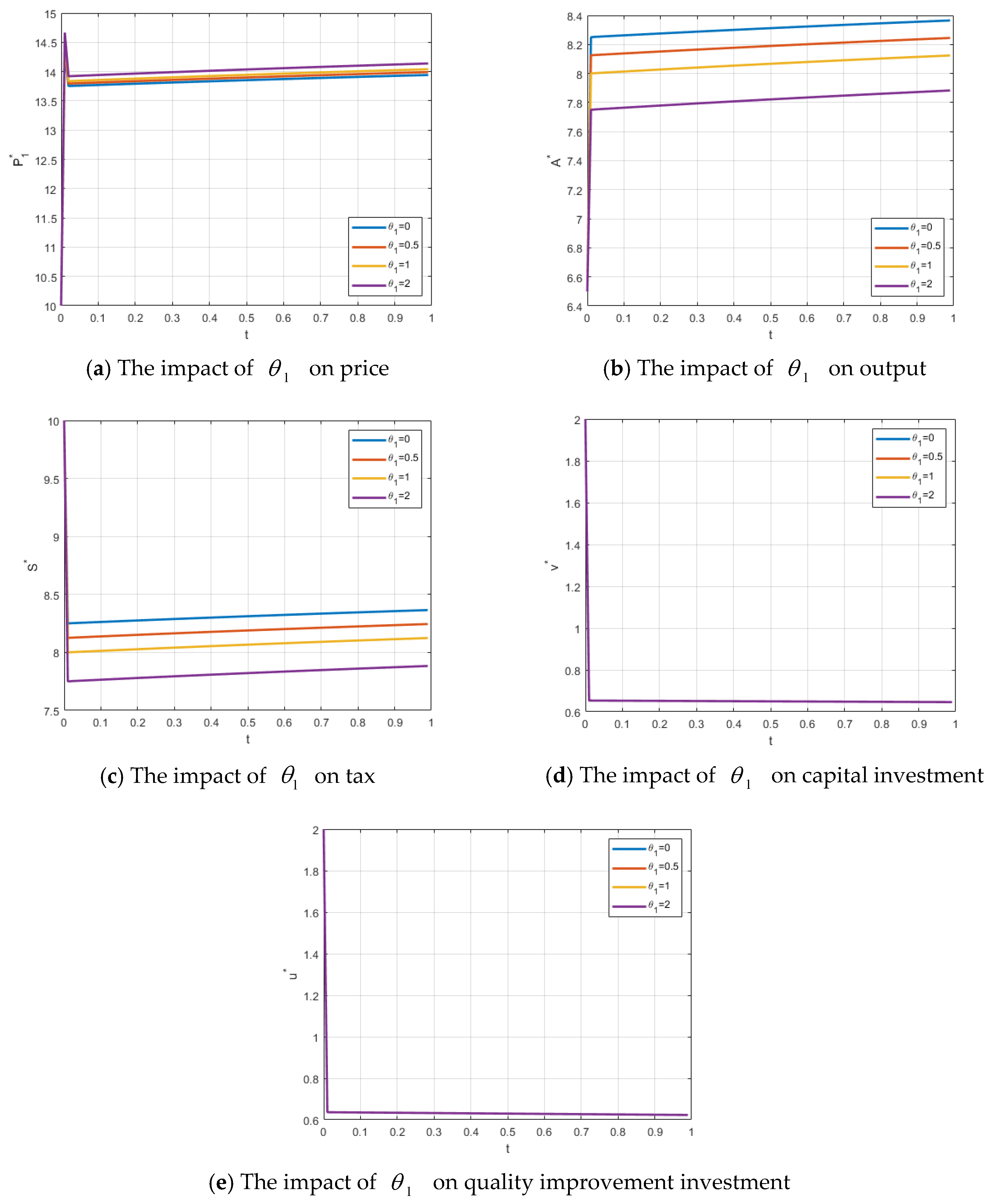
The effects of changes in
on the firm’s price, output, government tax, the firm’s capital investment, and local government food quality level are illustrated in
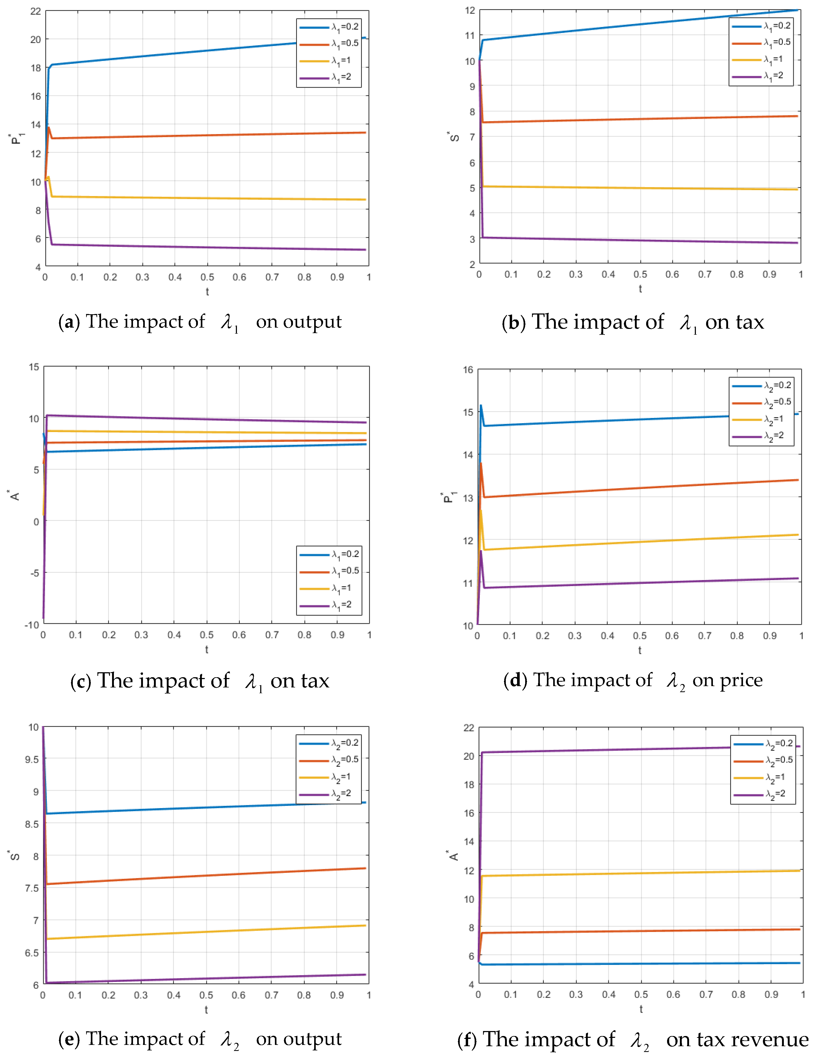
Figure 1a–e. As
increases, representing a rise in the reference price, the food-producing firm adjusts its price upward relative to competitors in order to maximize profit. The increase in the firm’s price reduces consumers’ willingness to purchase, leading to a decrease in market share. Since the price increase significantly affects market demand, it cannot fully offset the impact of reduced output, resulting in a decline in total firm profit. In response, the local government adopts tax incentives to lower the firm’s production cost, enabling the firm to reduce its price and increase output, thereby enhancing both firm profit and social welfare. Consequently, as
increases, the firm’s price rises while output and government tax decrease;
has no significant effect on the firm’s capital investment or the local government’s food quality improvement expenditure.
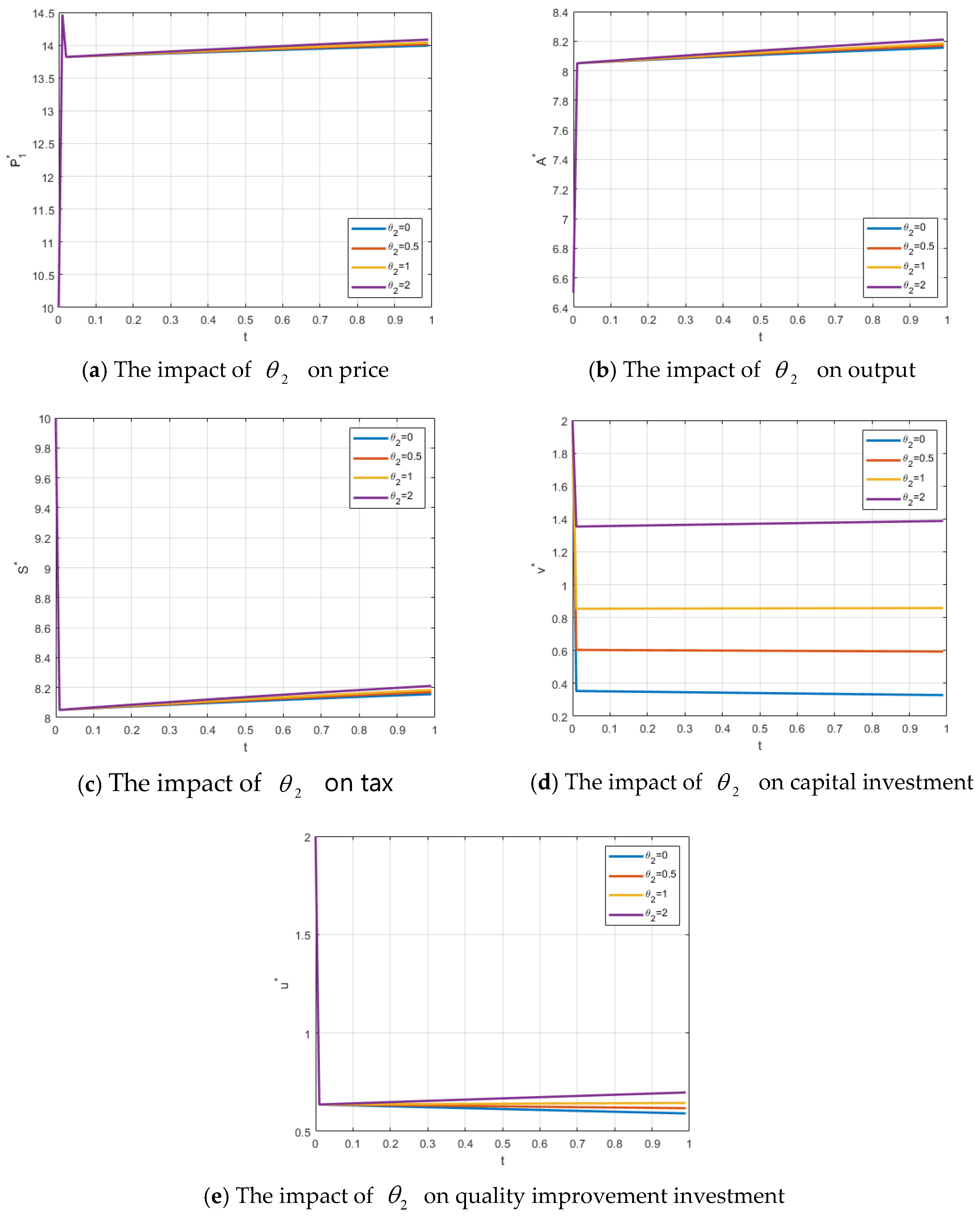
The effects of changes in
on the firm’s price, output, government tax revenue, the firm’s capital investment, and the local government’s food quality improvement investment are shown in
Figure 2a–e. As
increases, the firm’s price, output, and tax revenue increase correspondingly, although the magnitude of the effect is relatively small. In contrast, the impact on capital investment and food quality improvement investment is more pronounced, particularly for the required capital, which rises significantly. This is because enhancing green technology necessitates substantial financial investment, and improvements in technology also positively influence the local government’s investment in food quality improvement.
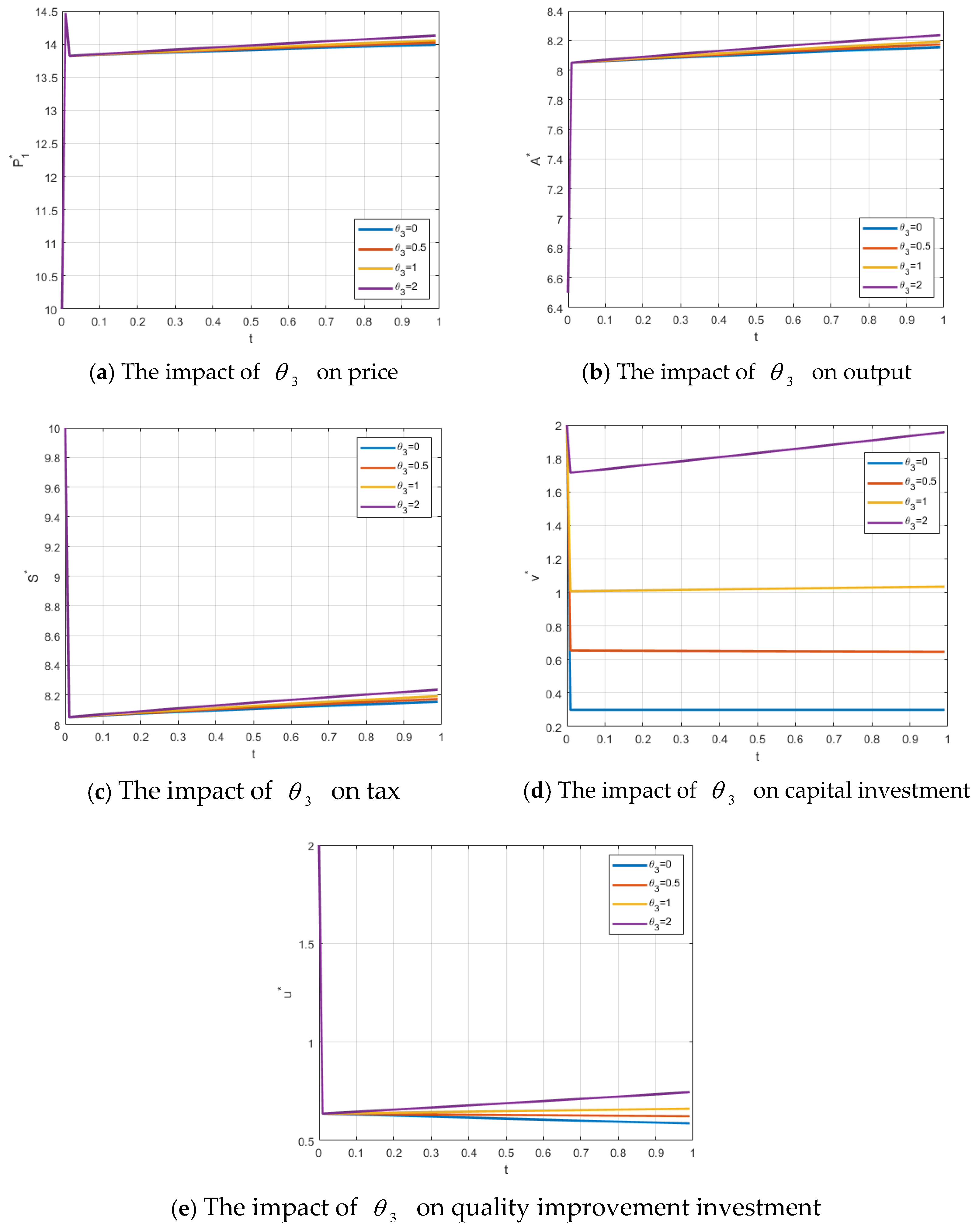
The effects of changes in
on the firm’s price, output, government tax revenue, the firm’s capital investment, and the local government’s food quality improvement level are shown in
Figure 3a–e. As
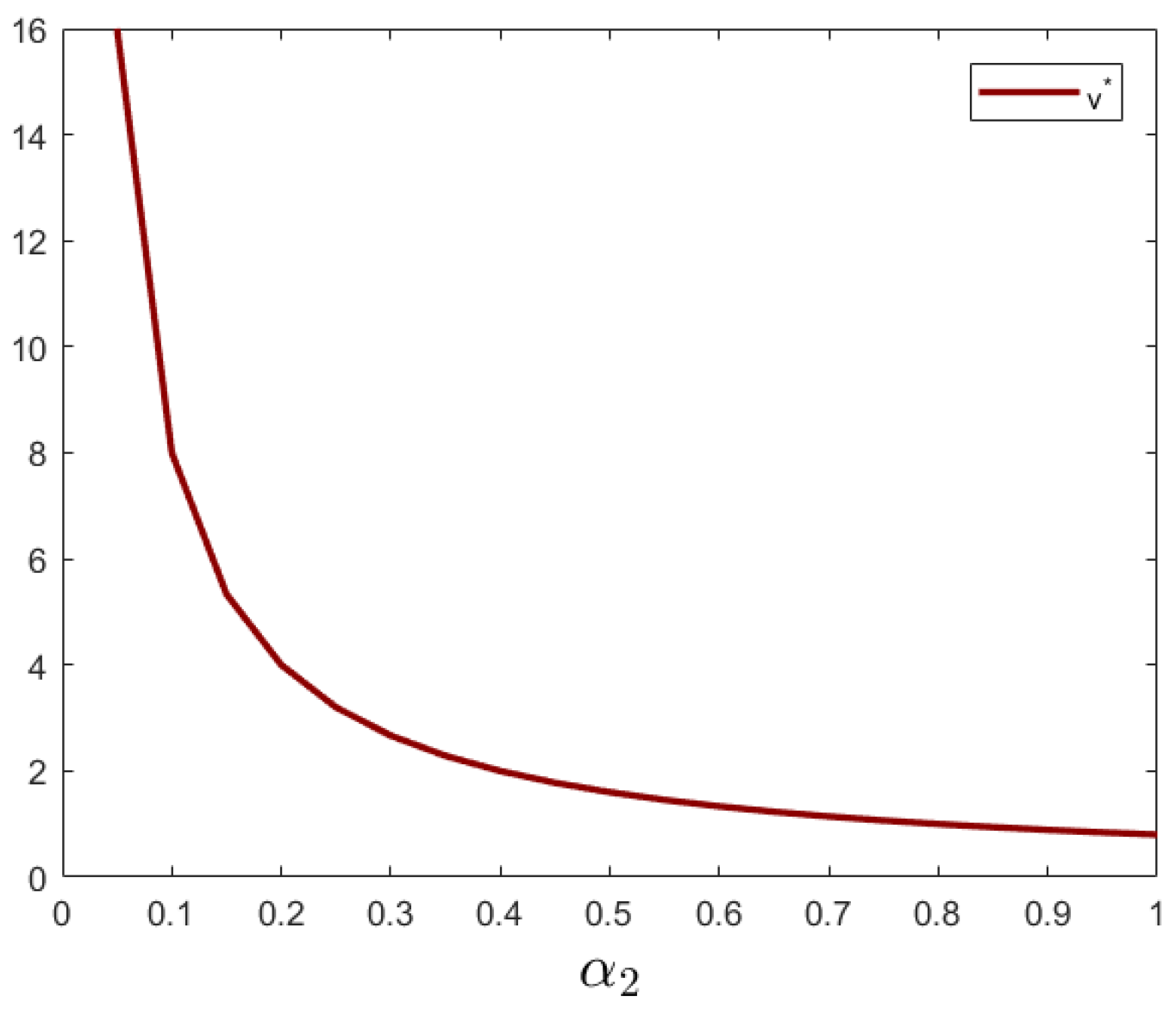
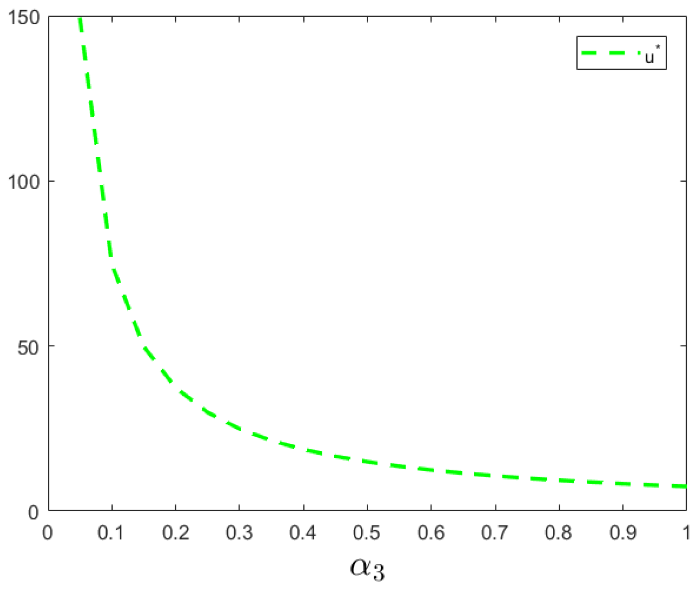
increases, indicating a higher impact factor of food quality level, there is a positive effect on the firm’s price, output, and tax revenue, although this is not particularly significant. In contrast, the effect on capital investment is much more pronounced, as substantial financial resources are required to enhance technological capabilities and achieve improvements in food quality.
The effects of changes in
on the firm’s price, output, government tax revenue, the firm’s capital investment, and the local government’s food quality level are illustrated in
Figure 4a–e. As
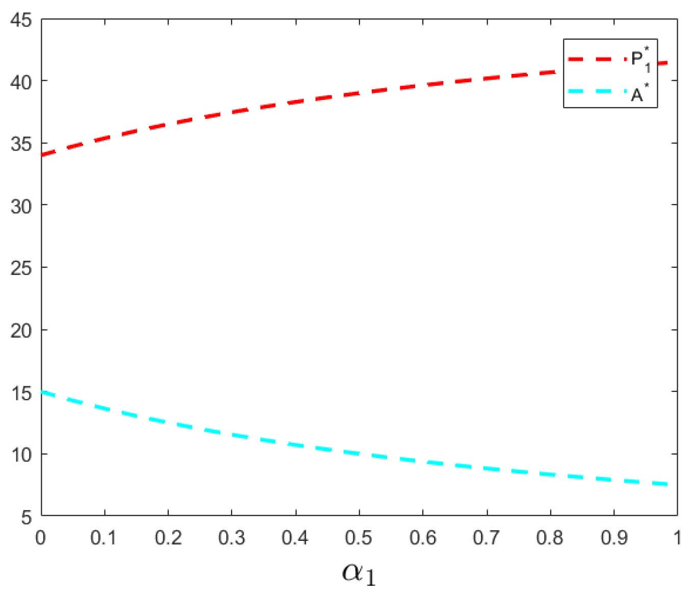
increases, there is no significant effect on the firm’s price, output, or tax revenue, but the firm’s capital investment shows a moderate increase, and the local government’s food quality level is significantly improved. This indicates that when local governments strengthen food quality supervision—such as by conducting irregular inspections, increasing penalties, and providing greater subsidies—social welfare in the jurisdiction is enhanced.
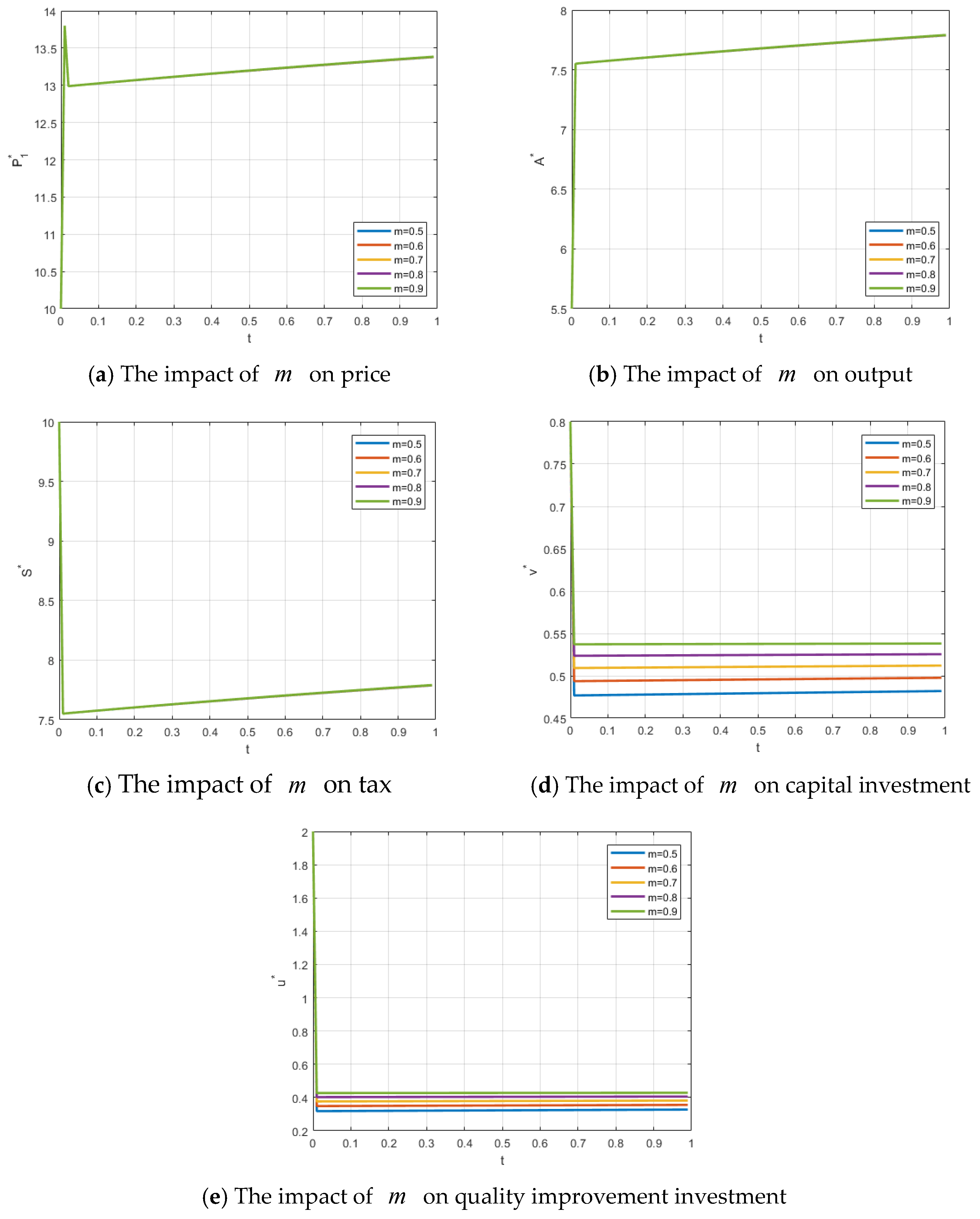
5.2. Effects of Food Quality Level on Price, Output, Tax, Capital Investment, and Quality Improvement Investment
The food quality level within the jurisdiction of the local government has a significant impact on government food quality investments. The higher the government’s investment in food quality, the higher the food quality level. At the same time, improvements in food quality also depend on the firm’s capital investment. By investing funds to enhance green technology, firms can further improve food quality. As shown in
Figure 5a–e, changes in food quality level do not have an immediate or significant impact on the firm’s price, output, or government tax revenue. However, over time, as consumers gradually recognize the improvement in food quality, their willingness to pay increases, which, in turn, drives upward trends in price, output, and tax revenue.
5.3. Effects of Demand Price Sensitivity and Price Difference Sensitivity on Price, Tax, and Production Quantity
As shown in
Figure 6a–f, both the demand price sensitivity coefficient and the price difference sensitivity have significant effects on product prices. With an increase in these sensitivity coefficients, market demand becomes more responsive to price, leading to a decrease in product prices. The reduction in product prices has a certain impact on government tax revenue, prompting the government to lower taxes to prevent high taxation from substantially reducing corporate profits. Meanwhile, the lower prices exert a positive effect on production quantity; as market demand rises, enterprises correspondingly increase their output.
5.4. Impact of Cost Coefficients ,
and on the Optimal Variables
An increase in the production cost coefficient
for food manufacturing enterprises raises their production costs. To maintain profits, firms increase product prices; however, higher prices reduce consumers’ willingness to pay, lowering purchasing power and market share, which, in turn, decreases demand and production volume (see
Figure 7). A higher green technology conversion cost coefficient
means that the cost of implementing green technologies is greater. Enterprises may find the cost prohibitive, and thus, reduce their investment in green technology, indicating a negative correlation between the technology cost coefficient and capital input (see
Figure 8). Similarly, an increase in the government’s food quality improvement cost coefficient
raises the expenditure required for enhancing food quality (see
Figure 9). When facing budget pressure, local governments may reduce their investment, leading to a decline in the level of food quality improvement input.
5.5. Sensitivity Analysis
As production costs increase, enterprises are likely to raise their product prices and reduce output, assuming other parameters remain constant, as shown in
Table 2.
As green tech conversion cost coefficient increases, enterprise’s green technology investment and food quality level go down, assuming other parameters remain constant, as shown in
Table 3.
As impact coefficient of enterprise’s green technology investment on food quality level
increase, enterprise’s green technology investment
rise and food quality level
is improved, assuming other parameters remain constant, as shown in
Table 4.
As consumer’s price sensitivity coefficient to food products
increase, enter- prise’s optimal product price
rise and enterprise’s optimal output
is improved, assuming other parameters remain constant, as shown in
Table 5.
As shadow price
increase, government’s food quality improvement investment
rise and food quality level
is improved, assuming other parameters remain constant, as shown in
Table 6.
6. Conclusions and Future Work
This study constructs a continuous-time coupled differential game model between the government and food-producing firms, analyzing the interactive strategies of the government’s optimal tax policy and food quality investment with the firms’ optimal pricing and capital investment. Firms determine their prices by referencing the prices of competitors’ products to achieve profit-maximizing strategies. Using the Stackelberg game approach, the strategies that maximize social welfare are obtained. The optimal dynamic strategies of the game participants are solved by applying Pontryagin’s maximum principle. Meanwhile, this research aims to analyze the influence of shadow prices on the decisions of local governments and firms. It does so by applying the backward differential equation method, as well as the impact of social welfare on the food quality level and government investment in food quality improvement within the local jurisdiction. The results indicate that incorporating social welfare considerations can help local governments enhance food quality and promote investment in food quality improvement by food-producing firms. The local government’s investment in food quality has a significant effect on the food quality level within its jurisdiction; the higher the government’s investment, the higher the food quality, and the food quality level is positively correlated with the firms’ investment in green technology. The price sensitivity of demand and sensitivity to price differences significantly affect market prices, fluctuating with changes in sensitivity coefficients. Specifically, as consumer price sensitivity increases, prices decrease, and the firms’ market share improves. Both the firms’ green technology investment and government food quality investment contribute to increasing social welfare.
This study constructs a continuous-time coupled differential game model between the government and food production enterprises. The analysis reveals the relationships between local government investment in food quality improvement, corporate investment in green technology, and food quality levels, as well as the impact of consumer price sensitivity on product pricing and market share, among other conclusions. Local governments can enhance food quality by increasing quality investments, guiding corporate behavior, and balancing market prices.
Increase investment in food quality improvement: Research indicates that local government investment in food quality significantly impacts the food quality level within their jurisdictions. Greater investment leads to higher food quality levels. Local governments should increase financial input into food quality improvement, such as purchasing more food testing equipment and building food quality supervision platforms. This will strengthen the supervision of the food production process and enhance overall food quality.
Guide enterprises to increase green technology investment: Since food quality levels are positively correlated with corporate investment in green technology, local governments can use policies such as tax incentives and subsidies to motivate enterprises to increase their green technology investments and improve food quality. Offering tax reductions to enterprises that actively invest in green technology can lower their production costs, increase profit margins, and thereby encourage greater financial commitment to advancing green technology.
Balance market prices: Consumer sensitivity to price and price differences has a noticeable impact on product pricing. Local governments can use these research findings to guide enterprises in setting reasonable prices. When consumers become more price-sensitive, enterprises should be encouraged to appropriately reduce product prices to increase market share. The government can also use subsidies to offset losses enterprises might incur due to price reductions, ensuring their profit margins are maintained.
Future research will continue in four directions. First, emphasis will be placed on collecting food safety data across the entire chain, including government, firms, media, social institutions, and consumers, to strengthen the study of multi-stakeholder coordinated governance mechanisms. Second, advanced technologies such as big data, artificial intelligence, and blockchain will be introduced to enhance the collection and fusion analysis of multi-source heterogeneous data, supporting precise behavioral modeling and dynamic simulation. Third, the theoretical model will be integrated with typical case studies and experimental research to refine model assumptions and parameter structures through the continuous accumulation of empirical data, thereby improving the practical interpretability and policy relevance of the research. Fourth, given regional disparities in economic development, which lead to varying local food safety governance requirements, subsequent studies will analyze the interaction between regional economic development and food safety governance.
