Diversity Constraint and Adaptive Graph Multi-View Functional Matrix Completion

Abstract

The integrity of real-time monitoring data is paramount to the accuracy of scientific research and the reliability of decision-making. However, data incompleteness arising from transmission interruptions or extreme weather disrupting equipment operations severely compromises the validity of statistical analyses and the stability of modelling. From a mathematical view, real-time monitoring data may be regarded as continuous functions, exhibiting intricate correlations and mutual influences between different indicators. Leveraging their inherent smoothness and interdependencies enables high-precision data imputation. Within the functional data analysis framework, this paper proposes a Diversity Constraint and Adaptive Graph Multi-View Functional Matrix Completion (DCAGMFMC) method. Integrating multi-view learning with an adaptive graph strategy, this approach comprehensively accounts for complex correlations between data from different views while extracting differential information across views, thereby enhancing information utilization and imputation accuracy. Random simulation experiments demonstrate that the DCAGMFMC method exhibits significant imputation advantages over classical methods such as KNN, HFI, SFI, MVNFMC, and GRMFMC. Furthermore, practical applications on meteorological datasets reveal that, compared to these imputation methods, the root mean square error (RMSE), mean absolute error (MAE), and normalized root mean square error (NRMSE) of the DCAGMVNFMC method decreased by an average of 39.11% to 59.15%, 54.50% to 71.97%, and 43.96% to 63.70%, respectively. It also demonstrated stable imputation performance across various meteorological indicators and missing data rates, exhibiting good adaptability and practical value.

1. Introduction

With the iterative advancement of data acquisition technologies, functional data exhibiting curve characteristics have proliferated across diverse domains. Examples include air pollutant concentration data and meteorological records. However, due to factors such as data transmission interruptions and extreme weather disrupting equipment operation, discrete sampling data often remains incomplete. This manifests as extensive random, strip-like, or block-shaped gaps, rendering data missingness a prevalent quality issue in functional datasets. Given that mainstream data analysis tools rely on complete datasets, imputation of missing values becomes a crucial preliminary step to ensure the accuracy of analytical outcomes.

In recent years, scholars have conducted in-depth research into functional data imputation methods. Existing imputation approaches [1] primarily encompass statistical analysis methods, machine learning methods, and deep learning methods [2]. Traditional statistical imputation techniques, such as mean-based imputation, perform poorly with functional data due to their failure to adequately account for the data’s curvilinear characteristics and the uncertainty inherent in missing patterns [3]. When non-linear relationships exist between variables, imputation based on linear regression yields suboptimal results [4]. For sparse functional data, Yao et al. [5] proposed Conditional Expectation Principal Component Estimation (PACE), leveraging principal component information. As a single imputation method, its performance is severely constrained by the data distribution and struggles to effectively capture non-linear relationships. The Multiple Imputation by Chain Equations (MICE) method proposed by Royston et al. [6] imputes missing values by generating multiple plausible yet distinct datasets. However, it remains sensitive to specific non-repetitive patterns. He et al. [7] introduced a functional multiple imputation approach under functional mixed-effects models, but this method imposes linearity constraints on the model assumptions and requires that the cause of data missingness be independent of the unobserved data itself. Ciarleglio et al. [8] combined MICE with functional regression to develop the fregMICE algorithm, although this approach is computationally intensive, necessitating advanced processing capabilities. When the growth rates of curve observations and sample size diverge, model parameter estimation lacks consistency, prompting the development of modern multiple imputation methods for functional data [9]. While multiple imputation is suitable for small-scale missingness in traditional datasets, it struggles to address large-scale missingness in high-dimensional matrices.

Furthermore, distance-based spatial imputation methods possess the ability to capture local characteristics in functional data analysis. Among these, inverse distance weighting (IDW) imputation stands as a classical approach, estimating missing values by calculating distance weights with respect to the adjacent sampling points. Its core assumption is that spatially proximate objects exhibit greater similarity; however, this method suffers from the flaw that weights tend towards infinity during close-range imputation [10]. Liu Yan et al. [11] further noted that such methods inadequately account for global data correlations. Spline imputation demonstrates significant advantages in handling missing values due to its smoothness and local adaptability. Its core principle involves constructing a globally smooth curve using piecewise low-order polynomials [12]. Compared to traditional linear imputation, this method better captures non-linear trends. However, spline imputation is relatively sensitive to data noise [11], meaning reliance solely on spline imputation may amplify the impact of high-frequency noise [13].

Traditional functional data imputation methods, such as soft functional matrix completion (SFI) [14] and hard functional matrix completion (HFI) [14], demonstrate certain efficacy in functional data imputation. However, they exhibit insufficient information extraction from the view of multivariate functional data [15]. KNN imputation [16], based on similarity metrics, performs imputation by identifying the K nearest samples to the missing data points, demonstrating excellent performance in preserving local data characteristics [17]. However, KNN imputation is sensitive to missing patterns. Research indicates that the regularized Expectation–Maximization (EM) method performs better when input variables exhibit little to no interdependence [18]. Matrix Factorization (MF) aims to discover a set of latent features (i.e., factor matrices), generating complete matrix data through linear combinations of these latent features to achieve missing value imputation [19]. To enhance MF’s ability to handle time series data, Yu et al. [20] introduced temporal regularization constraints, subsequently proposing a TRMF framework capable of data-driven temporal learning and forecasting. This method automatically learns dependencies between time series. Concurrently, deep learning approaches such as the time series imputation method proposed by He et al. [21] leverage joint tensor completion and recurrent neural networks to account for both temporal dependencies within individual time series and correlations between multiple time series. Furthermore, while the time series missing value estimation method based on recurrent neural networks [22] does not require assumptions about the underlying generative process of the data, it struggles to capture long-term dependencies. The Neural Context-Aware Anomaly Detection (NCAD) method proposed by Carmona et al. [23] excels at capturing long-term dependencies and complex patterns, but it suffers from high computational complexity and computational cost. Yoon et al. [24] proposed an iterative optimization of missing value imputation using a generator-discriminator game, though this approach demands substantial computational resources and requires large datasets.

In summary, when addressing the imputation of complex non-linear functional data, the aforementioned methods fail to adequately account for the functional characteristics of the data, the complexity of large-scale missing data, and the inter-variable correlations inherent in functional data. Functional Data Analysis (FDA) [25] represents discrete observations of data in functional form. By extracting multivariate data information and modelling from a functional data view, it can effectively reduce data noise when interpolating missing values [26]. Matrix completion, as an imputation method for handling large-scale data missingness, is widely adopted in practical applications [27]. Furthermore, research has demonstrated that the functional data recovery problem is equivalent to rank-constrained matrix completion [28]. Considering that functional data are typically multivariate, and that multi-view learning (MVL) outperforms single-view learning [29], utilizing information from multiple views can extract more accurate data features [30]. Methods for handling missing data within a multi-view learning framework can be categorized into two types: firstly, integrating consistency information across multiple views into matrix completion; secondly, treating the neighboring information of one view as complementary information or another view, thereby mutually providing neighboring information between different views and ultimately integrating complementary information from multiple views into matrix completion [31]. Therefore, within the functional data analysis framework, incorporating multi-view learning into matrix completion enables more effective imputation of missing data by extracting inter-view correlation information. For instance, Xue Jiao et al. [15] developed the Multi-View Non-Negative Functional Matrix Completion (MVNFMC) algorithm, which demonstrates superior data restoration performance compared to existing single-view functional data completion methods. Gao Haiyan and Ma Wenjuan [32] proposed a novel multi-view functional matrix completion method (GRMFMC), considering the higher-order domain relationships and complementary information between functional data views. This approach demonstrated superior imputation performance relative to other typical methods.

The aforementioned method achieved certain data imputation effects, but it only utilized the shared and complementary information within multi-view data, while neglecting the differential information between these views [33]. Therefore, fully leveraging the synergistic effects of multiple views can significantly enhance the precision and reliability of data feature extraction. Based on this, this study explores a more efficient functional data imputation method within the functional data analysis framework. This approach fully considers the multivariate and large-scale missing characteristics of functional data, as well as the differential information between views. Leveraging the principle that stronger vector orthogonality reduces information overlap, multi-view learning not only considers shared information across views but also enhances imputation accuracy by introducing diversity constraints between views to utilize their differential information [34,35]. This ensures the preservation of unique attributes from different views during multi-view data fusion. Capturing geometric properties through the spatial structure and local relationships between data samples can significantly enhance representation performance [36]. Specifically, this involves constructing a nearest neighbor graph to model sample relationships, utilizing the regularized decomposition process of the graph Laplacian matrix. However, data graphs constructed using traditional KNN methods may misclassify neighbors, thereby degrading clustering performance [33,37]. Furthermore, while higher similarity matrices yield more stable models, stricter similarity matrices diminish model generalization capability. Consequently, adaptively learning similarity matrices by maximizing information entropy enables more uniform information distribution within the similarity matrix, balancing model stability and generalization capability [38].

Given the intricate interdependencies and mutual influences among multi-view data, this paper integrates diversity constraints and adaptive graph learning into a functional matrix completion framework within the functional data analytics paradigm, incorporating multi-view learning. We propose a Diversity Constraint and Adaptive Graph Multi-View Functional Matrix Completion method (DCAGMFMC). This approach effectively addresses the limitations of existing functional data imputation methods in modelling complex nonlinear structures and integrating information across views by constructing a multi-view functional data representation framework and incorporating diversity constraints alongside adaptive graph learning strategies. It provides novel theoretical methods and technical pathways for missing data imputation in complex functional datasets. The principal contributions of this study are summarized as follows:

(1) Within the functional data analysis framework, integrating multi-view learning principles, we propose a novel multi-view functional matrix completion method. This approach pioneers the fusion of diversity constraints with adaptive graph learning within the functional matrix completion paradigm. By leveraging the diversity characteristics inherent in multi-view data, diversity constraints extract discriminative information across different views. By introducing information entropy, it adaptively learns similarity matrices, overcoming the shortcomings of traditional K-Nearest Neighbors methods in misclassifying neighbors during graph construction. Based on an adaptive graph strategy, it effectively captures complex correlations among data across views, deeply mining differential information between views. This significantly enhances data utilization efficiency, thereby substantially improving the imputation accuracy of functional data.

(2) Verification through random simulation experiments demonstrates that the DCAGMFMC method exhibits significant imputation advantages over classical methods such as KNN, HFI, SFI, MVNFMC, and GRMFMC, robustly proving its effectiveness and advancement in the field of functional data imputation.

(3) Practical application on meteorological datasets indicates that the DCAGMFMC method achieves substantial reductions in root mean square error (RMSE), mean absolute error (MAE), and normalized root mean square error (NRMSE). It also delivers stable imputation results across diverse meteorological indicators and varying levels of data missingness. This fully demonstrates the method’s excellent adaptability, practical value, and robust performance in repairing complex functional data gaps.

The structure of this article is as follows: Section 2 introduces prior work on curve fitting and functional matrix completion methods. Section 3 primarily details the formulation and optimization process of the DCAGMFMC method, including the convergence and time complexity of the submatrix update iteration. Section 4 presents simulation experiments and results analysis for the proposed method. Section 5 demonstrates practical applications of the proposed method. Section 6 summarizes the findings of the proposed method.

2. Related Work

2.1. Curve Fitting of Multi-View Functional Data

Dataset $X(t)=\{X_1(t),X_2(t),\cdots ,X_v(t),\cdots ,X_{n_v}(t)\}$ comprises $n_v$ views, with $X_v(t)$ representing the data for the $v$-th viewpoint. Each viewpoint $X_v(t)$ contains $n$ samples, whose observational dimensions are denoted as $m_v$. Within $X_v(t)=\{x_1^v(t),x_2^v(t),\cdots ,x_n^v(t)\}$, there are $n$ curves in total. The curve for the $v$-th viewpoint is $x_i^v(t)(i=1,2,\cdots ,n)$. The $j$-th discrete observation value ${\tilde{y}}_{ij}^v$ of the $i$-th curve under the $v$-th viewpoint is generated by the general regression model Equation (1):

$${\tilde{y}}_{ij}^v=x_i^v(t_{ij})+{\epsilon }_{ij}^v$$

(1)

where $v$ denotes the random error term, and $j=1,2,\cdots ,m_v$ represents the observation time points over the time interval $T$. Consequently, $x_i^v(t)$ can be approximated by the following finite-dimensional Gaussian function expansion:

$$x_i^v(t)\approx {\displaystyle \sum _{l=1}^r{\alpha }_{il}^v}{\phi }_{il}^v(t)={\mathit{\phi }}_i^v{(t)}^T{\alpha }_i^v$$

(2)

Given a set of basis vectors ${\mathit{\phi }}_i^v(t)={({\phi }_{i1}^v(t),{\phi }_{i2}^v(t),\cdots ,{\phi }_{ir}^v(t))}^T$ and an estimated coefficient vector ${\mathit{\alpha }}_i^v={({\alpha }_{i1}^v,{\alpha }_{i2}^v,\cdots ,{\alpha }_{ir}^v)}^T$, Equations (1) and (2) can be expressed in matrix form respectively as follows:

$${\tilde{X}}_v^{+}\approx {\Phi }_v{A}_v$$

(3)

$${\tilde{Y}}_v^{+}={\Phi }_v{A}_v+E_v$$

(4)

where ${\Phi }_v={({\mathit{\phi }}_1^v(t),{\mathit{\phi }}_2^v(t),\cdots ,{\mathit{\phi }}_{m_v}^v(t))}^T$ denotes the basis functions computed at the observation time point, and represents the basis function matrix shared across all viewpoints, $A_v={({\alpha }_1^v,{\alpha }_2^v,\cdots ,{\alpha }_n^v)}^T$, $E_v=({\epsilon }_1^v,{\epsilon }_2^v,\cdots ,{\epsilon }_n^v)$, ${\epsilon }_i^v=({\epsilon }_{i1}^v,{\epsilon }_{i2}^v,\cdots ,{\epsilon }_{i{m}_v}^v)$.

2.2. Multi-View Functional Matrix Completion

Given $Y=\{{\tilde{Y}}_1^{+},{\tilde{Y}}_2^{+},\cdots ,{\tilde{Y}}_{n_v}^{+}\}$ as a multi-view data matrix, the symbol ${(·)}^{+}$ denotes taking the positive part of the matrix, ensuring the non-negativity of the observed data, the fundamental objective function based on multi-view functional matrix completion [15] is:

$$\underset{U_v,V_v\ge 0}{\min }\left\{{\displaystyle \sum _{v=1}^{n_v}{\theta }_v}{‖O\odot ({\tilde{Y}}_v^{+}-\Phi U_v{V}_v^T)‖}_F^2\right\}$$

(5)

Here, ${\theta }_v$ denotes the weighting parameter for different views, $\odot$ represents the Hadamard matrix product, and $\Phi \in {ℝ}^{m\times r}$ and $O\in {ℝ}^{m\times n}$ are projection matrices of the same type as ${\tilde{Y}}_v^{+}$. Specifically, if the entries in ${\tilde{Y}}_v^{+}$ are observable, then $O_{ij}=1$; otherwise, $O_{ij}=0$, $U_v\in {ℝ}^{r\times \mathrm{d}}$, and $V_v\in {ℝ}^{n\times d}$ respectively denote the basis matrix and coefficient matrix for the $v$-th view.

3. Methodology

3.1. DCAGMFMC

Multi-view data possess richer content than single-view data, exhibiting multiple features. However, existing methods overly rely on shared information across different views, neglecting the distinctiveness between each view. This leads to information loss and underutilization. By learning constrained coefficient matrices, we obtain diversified coefficient matrices, thereby extracting complementary information between different views of the same sample. Let the $i$-th coefficient vector corresponding to the $v$-th view be denoted as c, where $v=1,2,\cdots ,n_v$, $i=1,2,\cdots n$, and the $i$-th coefficient vector corresponding to the $w$-th view be denoted as $V_{wi}\in {ℝ}^d$, where $w=1,2,\cdots ,n_v$, $i=1,2,\cdots n$. The stronger the orthogonality between two vectors, the more diverse and non-redundant the information or features they carry [34]. Therefore, by minimizing the inner product between two coefficient vectors from different views, we extract the unique information specific to each view. For $n$ vectors, we have:

$$\min {\displaystyle \sum _{i=1}^n{v}_{vi}^T}{v}_{wi}=\min \mathrm{tr}(V_v{V}_w^T)$$

(6)

To understand the differences in information between the coefficient matrices of the $v$-th and other views across different samples, the diversity constraint can be expressed as:

$$\min {\displaystyle \sum _{v=1}^{n_v}{\displaystyle \sum _{w=1}^{n_v}\mathrm{tr}(V_v{V}_w^T)}}$$

(7)

Concurrently, high-dimensional spaces exhibit data redundancy. Sampling data from low-dimensional manifolds embedded within these high-dimensional spaces [36] enables the extraction of key information while reducing computational complexity. Owing to the multivariate nature of functional data, samples sharing identical views exhibit strong interconnections, revealing inherent patterns within the data. Consequently, preserving the intrinsic geometric structure of functional data is paramount. As a dimension reduction and feature extraction technique, NMF focuses on numerical relationships within data while neglecting its geometric structure. Graph-based NMF captures this geometric structure, with the graph regularization expressed as:

$$\min {\displaystyle \frac{1}{2}}{\displaystyle \sum _{i=1}^n{\displaystyle \sum _{j=1}^n{‖v_{vi}-v_{vj}‖}_2^2}{s}_{vij}=\min \mathrm{tr}(V_v^T{L}_v{V}_v)}$$

(8)

Here, $S_v$ denotes the similarity matrix, representing the degree of similarity between data points. $L_v={\mathit{D}}_v-W_v$ denotes the Laplacian matrix. ${\mathit{D}}_v$ is the degree matrix, $W_v$ is the adjacency matrix, $D_{vii}={\displaystyle {\sum }_{j=1}^n{w}_{vij}}$, and since $S_v$ is an asymmetric matrix, let $W_v=(S_v+S_v^T)/2$.

For learning similarity matrices, the KNN method is commonly employed. However, if the majority of data points cluster near the intersection of multiple subspaces, KNN fails to partition these subspaces correctly. Furthermore, the KNN approach necessitates frequent adjustments to the number of neighbors [39]. In information theory, information entropy serves as a physical quantity describing the unpredictability of information content. Let information $q=(q_1,q_2,\cdots ,q_n)$ consist of $n$ sources, with $q_i$ denoting the probability of the $i$-th source. The information entropy $q$ can be expressed as:

$$y={\displaystyle \sum _{i=1}^n{q}_i\log \frac{1}{q_i}}$$

(9)

The higher the similarity, the more stable the model; however, a stricter similarity matrix reduces the model’s generalization capability. In Equation (9), greater entropy indicates richer information content within the matrix. By maximizing the entropy of the similarity matrix with temperature parameters, one can effectively learn the similarity matrix, promoting more uniform information distribution within the matrix and balancing model stability with generalization capability [38]. Consequently, the information-entropy-based adaptive graph method can overcome the drawback of misclassifying neighbors. Its mathematical expression is:

$$\max {\displaystyle \sum _{i=1}^n{\displaystyle \sum _{j=1}^n{s}_{vij}\log \left(1/s_{vij}^{\tau }\right)}}\mathrm{s.t.}{\displaystyle \sum _{j=1}^n{s}_{vij}}=1,s_{vij}\ge 0$$

(10)

Here, the temperature parameter $\tau$ controls the strength of entropy.

Combining diversity constraints and adaptive graphs [40], we propose a multi-view functional matrix completion model based on diversity constraints and adaptive graphs.

$$\begin{array}{ll}\min & {\displaystyle \sum _{v=1}^{n_v}{\theta }_v{‖O\odot ({\tilde{Y}}_v^{+}-\Phi U_v{V}_v^T)‖}_F^2+2{\theta }_{vs}{\displaystyle \sum _{v=1}^{n_v}{\displaystyle \sum _{w=1}^{n_v}\mathrm{tr}(V_v{V}_w^T)}}}\\ & +\mu {\displaystyle \sum _{v=1}^{n_v}\mathrm{tr}(V_v^T{L}_v{V}_v)+\lambda {\displaystyle \sum _{i=1}^n{\displaystyle \sum _{j=1}^n{s}_{vij}\log s_{vij}^{\tau }}}}\\ \mathrm{s.t.}& U_v\ge 0,\hspace{1em}{V}_v\ge 0,\hspace{1em}{\displaystyle \sum _{j=1}^n{s}_{vij}=1,\hspace{1em}{s}_{vij}\ge 0}\end{array}$$

(11)

Here, $v=1,2,\cdots ,n_v$, ${\theta }_{vs},\mu ,\lambda \ge 0$ are parameters adjusting the weighting relationships between components. The first term constitutes the fundamental objective function for multi-view functional matrix completion; the second term represents a diversity constraint designed to integrate disparate information across different sites; the third and fourth terms form an adaptive graph constraint. The fourth component adapts to learn similarity matrices by maximizing their entropy, while the third component incorporates the geometric structure of the data through the graph Laplacian matrix. Figure 1 presents the schematic diagram of the proposed DCAGMFMC method.

3.2. Optimization Algorithm

The non-convexity of objective function (11) with respect to $U_v$ and $V_v$ poses challenges for global optimization. To address this issue, this paper employs an alternating minimization strategy to solve Equation (11). Each variable is updated while holding the others constant. The augmented Lagrangian function for (11) is given by:

$$\begin{array}{ll}\mathcal{L}=& {\displaystyle \sum _{v=1}^{n_v}{\theta }_v{‖O\odot ({\tilde{Y}}_v^{+}-\Phi U_v{V}_v^T)‖}_F^2+2{\theta }_{vs}{\displaystyle \sum _{v=1}^{n_v}{\displaystyle \sum _{w=1}^{n_v}\mathrm{tr}(V_v{V}_w^T)}}}\\ & +\mu {\displaystyle \sum _{v=1}^{n_v}\mathrm{tr}(V_v^T{L}_v{V}_v)}+\lambda {\displaystyle \sum _{i=1}^n{\displaystyle \sum _{j=1}^n{s}_{vij}\log s_{vij}^{\tau }}}-\mathrm{tr}({\Psi }_v^T{U}_v)\\ & -\mathrm{tr}({\Gamma }_v^T{V}_v)-{\displaystyle \sum _{i=1}^n{\xi }_i({\displaystyle \sum _{j=1}^n{s}_{vij}-1})-{\displaystyle \sum _{i=1}^n{\displaystyle \sum _{j=1}^n{\pi }_{ij}{s}_{vij}}}}\end{array}$$

(12)

(1) Fixing $V_v$ and $S_v$, update $U_v$. Given $V_v$ and $S_v$, find a $U_v$ that better reconstructs the observed data matrix ${\tilde{Y}}_v^{+}$. The part of Equation (12) concerning $U_v$ simplifies to:

$${\mathcal{L}}_1={\theta }_v\mathrm{tr}\left(O\odot ({\tilde{Y}}_v^{+}-\Phi U_v{V}_v^T)\right){\left(O\odot ({\tilde{Y}}_v^{+}-\Phi U_v{V}_v^T)\right)}^T-\mathrm{tr}({\Psi }_v^T{U}_v)$$

(13)

Taking the partial derivative of Equation (13) with respect to $U_v$ and setting it equal to zero yields:

$$-2{\theta }_v{\Phi }^T(O\odot {\tilde{Y}}_v^{+})V_v+2{\theta }_v{\Phi }^T(O\odot \Phi U_v{V}_v^T)V_v={\Psi }_v$$

(14)

According to the KKT conditions, satisfying ${\Psi }_v\odot U_v=0$, we have:

$${\left(-2{\theta }_v{\Phi }^T(O\odot {\tilde{Y}}_v^{+})V_v+2{\theta }_v{\Phi }^T(O\odot \Phi U_v{V}_v^T)V_v\right)}_{ij}\odot U_{vij}=0$$

(15)

Thus, the updated formula for $U_v$ is obtained as follows:

$$U_{vij}\leftarrow U_{vij}\sqrt{{\displaystyle \frac{{\left({\Phi }^T(O\odot {\tilde{Y}}_v^{+})V_v\right)}_{ij}}{{\left({\Phi }^T(O\odot \Phi U_v{V}_v^T)V_v\right)}_{ij}}}}$$

(16)

(2) Fixing $U_v$ and $S_v$, update $V_v$. The part of Equation (12) concerning $V_v$ simplifies to:

$$\begin{array}{ll}{\mathcal{L}}_2=& {\theta }_v\mathrm{tr}\left(O\odot ({\tilde{Y}}_v^{+}-\Phi U_v{V}_v^T)\right){\left(O\odot ({\tilde{Y}}_v^{+}-\Phi U_v{V}_v^T)\right)}^T\\ & +2{\theta }_{vs}{\displaystyle \sum _{w=1}^{n_v}\mathrm{tr}(V_v{V}_w^T)}+\mu \mathrm{tr}(V_v^T{L}_v{V}_v)-\mathrm{tr}({\Gamma }_v^T{V}_v)\end{array}$$

(17)

Taking the partial derivative of Equation (17) with respect to $V_v$ and setting it to zero and combining with the KKT conditions satisfying ${\Gamma }_v\odot V_v=0$ yields:

$$\begin{array}{l}(-2{\theta }_v(O^T\odot {\tilde{Y}}_v^{+T})\Phi U_v+2{\theta }_v(O^T\odot V_v{U}_v^T{\Phi }^T)\Phi U_v\\ +2{\theta }_{vs}{\displaystyle \sum _{w=1,w\ne v}^{n_v}{V}_w+4{\theta }_{vs}{V}_v+2\mu ({\mathit{D}}_v-W_v)V_v}{)}_{ij}\odot V_{vij}=0\end{array}$$

(18)

The updated formula for $V_v$ is:

$$V_{vij}\leftarrow V_{vij}\sqrt{{\displaystyle \frac{{\left({\theta }_v(O^T\odot {\tilde{Y}}_v^{+T})\Phi U_v+\mu W_v{V}_v\right)}_{ij}}{{\left({\theta }_v(O^T\odot V_v{U}_v^T{\Phi }^T)\Phi U_v+{\theta }_{vs}{\displaystyle \sum _{w=1,w\ne v}^{n_v}{V}_w+2{\theta }_{vs}{V}_v+\mu {\mathit{D}}_v{V}_v}\right)}_{ij}}}}$$

(19)

where Equation (19) updates the latent representation $V_v$, shared across all viewpoints, integrating multi-view information. The diversity constraint is embodied by the ${\theta }_{vs}{\displaystyle \sum _{w=1,w\ne v}^{n_v}{V}_w+2{\theta }_{vs}{V}_v}$ term, which ensures the latent representation $V_v$ of the current viewpoint remains orthogonal to representations from all other viewpoints. This captures complementary information and prevents learning redundant features. Image regularization is embodied by the $\mu W_v{V}_v$ and $\mu {\mathit{D}}_v{V}_v$ terms.

(3) Fixing $U_v$ and $V_v$, update $S_v$. The augmented Lagrangian function with respect to $S_v$ is:

$${\mathcal{L}}_3=2\mathrm{tr}(V_v^T{L}_v{V}_v)+2\lambda {\displaystyle \sum _{i=1}^n{\displaystyle \sum _{j=1}^n{s}_{vij}\log s_{vij}^{\tau }}}-{\displaystyle \sum _{i=1}^n{\xi }_i({\displaystyle \sum _{j=1}^n{s}_{vij}-1})-{\displaystyle \sum _{i=1}^n{\displaystyle \sum _{j=1}^n{\pi }_{ij}{s}_{vij}}}}$$

(20)

Taking the partial derivative with respect to $S_v$ in Equation (20) and setting it equal to zero yields:

$${‖v_{vi}-v_{vj}‖}_2^2+2\lambda \tau (\log s_{vij}+1)-{\xi }_i-{\pi }_{ij}=0$$

(21)

Applying the KKT condition ${\pi }_{ij}{s}_{vij}=0$, when $s_{vij}>0$, then ${\pi }_{ij}=0$, it follows that:

$${‖v_{vi}-v_{vj}‖}_2^2+2\lambda \tau (\log s_{vij}+1)-{\xi }_i=0$$

(22)

Thereby:

$$\begin{array}{ll}{s}_{vij}& =\exp \left\{({\xi }_i-2\lambda \tau )/2\lambda \tau \right\}\exp \left\{-\left({‖v_{vi}-v_{vj}‖}_2^2\right)/2\lambda \tau \right\}\\ & ={\rho }_i\exp \left\{-\left({‖v_{vi}-v_{vj}‖}_2^2\right)/2\lambda \tau \right\}\end{array}$$

(23)

where ${\rho }_i=\exp \left\{({\xi }_i-2\lambda \tau )/2\lambda \tau \right\}$. Given that ${\displaystyle \sum _{j=1}^n{s}_{vij}=1}$, the calculation of ${\rho }_i$ yields:

$${\rho }_i=1/{\displaystyle \sum _{j=1}^n\exp \left\{-\left({‖v_{vi}-v_{vj}‖}_2^2\right)/2\lambda \tau \right\}}$$

(24)

Combining Equation (24), the updated formula for $S_v$ is obtained as:

$$s_{vij}\leftarrow \exp \left\{-\left({‖v_{vi}-v_{vj}‖}_2^2\right)/2\lambda \tau \right\}/{\displaystyle \sum _{j=1}^n\exp \left\{-\left({‖v_{vi}-v_{vj}‖}_2^2\right)/2\lambda \tau \right\}}$$

(25)

3.3. Convergence Analysis

Below, we conduct a convergence analysis of the update formulas for $U_v$, $V_v$, and $S_v$ in Equations (16), (19), and (25), that is, prove Theorem 1. Our optimization algorithm can be incorporated into the Block Coordinate Descent (BCD) framework [41]. Within this framework, since each subproblem is solved precisely and ensures sufficient descent of the objective function, the sequence generated by the algorithm converges to a stationary point of the objective function according to its convergence theory.

Theorem 1.

Given initial values, applying the update rules derived in this study (Equations (16), (19), and (25)) for optimization results in the objective function (11) decreasing monotonically at each iteration.

Proof. 

According to the convergence theory established by Tseng [41], if solving each subproblem leads to a sufficient decrease in the objective function value, then any limit point of the sequence is a stationary point of the objective function. The convergence of updates to expressions (16), (19) and (25) is demonstrated by con structing auxiliary functions. In each update, terms related to $U_v$ are retained from the objective function expression (11), while unrelated terms are discarded.

$$\mathcal{L}(U_v)=\mathrm{tr}(U_v^T{\Phi }^T(O\odot \Phi U_v{V}_v^T)V_v-2U_v^T{\Phi }^T(O\odot {\tilde{Y}}_v^{+})V_v)$$

(26)

The auxiliary function $G(U_v,U_v^t)$ is constructed based on the control inequality commonly used in the MM algorithm [42]. For terms of the form $x^2$, we employ the inequality $x^2/y\ge 2x-y$, where $y>0$. For terms of the form $-\log x$, we employ the inequality $-\log x\ge 1-x/y+\log y$. Replacing each term $\mathcal{L}(U_v)$ with its upper bound at $U_v=U_v^t$ yields the expression for the auxiliary function $G(U_v,U_v^t)$ as follows:

$$\begin{array}{ll}G(U_v,U_v^t)=& {\displaystyle \sum _{i,j}\frac{{\left({\Phi }^T(O\odot \Phi U_v^t{V}_v^T)V_v\right)}_{ij}{U}_{vij}^2}{U_{vij}^t}}\\ & -2{\displaystyle \sum _{i,j}{\left({\Phi }^T(O\odot {\tilde{Y}}_v^{+})V_v\right)}_{ij}{U}_{vij}^t(1+\log \frac{U_{vij}}{U_{vij}^t})}\end{array}$$

(27)

This construction ensures that when $U_v=U_v^t$, all inequalities hold with equality, hence $G(U_v,U_v)=\mathcal{L}(U_v)$. For other values of $U_v$, since each term is an upper bound, we have $G(U_v,U_v^t)\ge \mathcal{L}(U_v)$ if $U_v^{t+1}$ is chosen such that:

$$U_v^{t+1}=\underset{t}{\arg \min }G(U_v,U_v^t)$$

(28)

Established, it is evident that $\mathcal{L}(U_v)$ is monotonically decreasing, with:

$$G(U_v^{t+1},U_v^{t+1})\le G(U_v^{t+1},U_v^t)\le G(U_v^t,U_v^t)$$

(29)

To minimize the auxiliary function Equation (27), solve for $U_v^{t+1}$ subject to the constraint in Equation (28). Taking the partial derivative of Equation (27) with respect to $U_{vij}$ and setting it to zero, while substituting $U_{vij}$ with $U_{vij}^{t+1}$, yields:

$${\displaystyle \frac{{\left({\Phi }^T(O\odot \Phi U_v^t{V}_v^T)V_v\right)}_{ij}{U}_{vij}^{t+1}}{U_{vij}^t}}={\left({\Phi }^T(O\odot {\tilde{Y}}_v^{+})V_v\right)}_{ij}{\displaystyle \frac{U_{vij}^t}{U_{vij}^{t+1}}}$$

(30)

Furthermore:

$$U_{vij}^{t+1}=U_{vij}^t\sqrt{{\displaystyle \frac{{\left({\Phi }^T(O\odot {\tilde{Y}}_v^{+})V_v\right)}_{ij}}{{\left({\Phi }^T(O\odot \Phi U_v^t{V}_v^T)V_v\right)}_{ij}}}}$$

(31)

Hence, Equation (31) is derived as the update rule Equation (16) for $U_v$.

Below we prove the convergence of the update rule Equation (19) for $V_v$. In Equation (11), only the terms relating to $V_v$ are retained:

$$\begin{array}{ll}\mathcal{L}(V_v)=& \mathrm{tr}(2{\theta }_v{V}_v^T(O^T\odot {\tilde{Y}}_v^{+T})\Phi U_v-2{\theta }_v(O^T\odot V_v{U}_v^T{\Phi }^T)\Phi U_v)\\ & +2{\theta }_{vs}{\displaystyle \sum _{w=1}^{n_v}\mathrm{tr}(V_v{V}_w^T)}+\mu \mathrm{tr}(V_v^T{L}_v{V}_v)\end{array}$$

(32)

Similarly, construct auxiliary function $G(V_v,V_v^t)$ of $\mathcal{L}(V_v)$, defined as:

$$\begin{array}{ll}G(V_v,V_v^t)=& {\displaystyle \sum _{i,j}\frac{{\left({\theta }_v(O^T\odot V_v{U}_v^T{\Phi }^T)\Phi U_v+{\theta }_{vs}{\displaystyle \sum _{w=1,w\ne v}^{n_v}{V}_w}+2{\theta }_{vs}{V}_v+\mu {\mathit{D}}_v{V}_v\right)}_{ij}{V}_{vij}^2}{V_{vij}^t}}\\ & -2{\theta }_v{\displaystyle \sum _{i,j}{\left((O^T\odot {\tilde{Y}}_v^{+T})\Phi U_v+\mu W_v{V}_v\right)}_{ij}{V}_{vij}^t(1+\log \frac{V_{vij}}{V_{vij}^t})}\end{array}$$

(33)

Then, conditions $G(V_v,V_v)=\mathcal{L}(V_v)$ and $G(V_v,V_v^t)\ge \mathcal{L}(V_v)$ are satisfied. If $V_v^{t+1}$ is chosen such that:

$$V_v^{t+1}=\arg \min G(V_v,V_v^t)$$

(34)

This established, it is evident that $\mathcal{L}(V_v)$ is monotonically decreasing, with:

$$G(V_v^{t+1},V_v^{t+1})\le G(V_v^{t+1},V_v^t)\le G(V_v^t,V_v^t)$$

(35)

To minimize the auxiliary function Equation (33), solve for $V_v^{t+1}$ subject to the constraint in Equation (34). Taking the partial derivative of Equation (34) with respect to $V_{vij}$ and setting it to zero yields:

$${\left({\theta }_v(O^T\odot {\tilde{Y}}_v^{+T})\Phi U_v+\mu W_v{V}_v\right)}_{ij}{\displaystyle \frac{V_{vij}^t}{V_{vij}^{t+1}}}={\displaystyle \frac{{\left({\theta }_v(O^T\odot V_v{U}_v^T{\Phi }^T)\Phi U_v+{\theta }_{vs}{\displaystyle \sum _{w=1,w\ne v}^{n_v}{V}_w}+2{\theta }_{vs}{V}_v+\mu {\mathit{D}}_v{V}_v\right)}_{ij}}{V_{vij}^t}}{V}_{vij}^{t+1}$$

(36)

Thereby:

$$V_{vij}^{t+1}\leftarrow V_{vij}^t\sqrt{{\displaystyle \frac{{\left({\theta }_v(O^T\odot {\tilde{Y}}_v^{+T})\Phi U_v+\mu W_v{V}_v\right)}_{ij}}{{\left({\theta }_v(O^T\odot V_v{U}_v^T{\Phi }^T)\Phi U_v+{\theta }_{vs}{\displaystyle \sum _{w=1,w\ne v}^{n_v}{V}_w}+2{\theta }_{vs}{V}_v+\mu {\mathit{D}}_v{V}_v\right)}_{ij}}}}$$

(37)

Hence, Equation (37) is derived as the update rule (19) for $U_v$. Similarly, the update rule Equation (25) for $S_v$ can be demonstrated. □

In summary, the specific implementation steps of the DCAGMFMC method are summarized in Algorithm 1 as follows:

Algorithm 1. DCAGMFMC

Input: Multi-view data matrix $Y$, parameters ${\theta }_v,{\theta }_{vs},\mu ,\lambda ,{\epsilon }_0={10}^{-7}$, iteration count $t$ Output: $\{U_1^{t+1},U_2^{t+1},\cdots ,U_{n_v}^{t+1}\}$ and $\{V_1^{t+1},V_2^{t+1},\cdots ,V_{n_v}^{t+1}\}$. 1. Generate random values for $U_v^0$ and $V_v^0$, then initialize $S_v^0$ according to Equation (25); 2. Fixing $V_v$ and $S_v$, update $U_v^{t+1}$ according to Equation (16); 3. Fixing $U_v$ and $S_v$, update $V_v^{t+1}$ according to Equation (19); 4. Fixing $U_v$ and $V_v$, update $S_v^{t+1}$ according to Equation (25); 5. Repeat the aforementioned optimization steps (steps 2–4) until ${‖U_v^{t+1}{V}_v^{t{+1}^T}-U_v^t{V}_v^{t^T}‖}^2/{‖U_v^t{V}_v^{t^T}‖}^2\le {\epsilon }_0$ is achieved.

Given the global non-convexity of the objective function (11), the convergence of the algorithm to a fixed point depends on the initialization choice, and multiple local minima may exist. To mitigate the potential impact of this issue on algorithm performance and the reliability of conclusions, and to obtain stable, robust solutions, we will implement the following measures in the numerical experimental design:

(1) Multiple Random Initializations: In each independent experiment run, the weight matrices $U_v$ and $V_v$ are initialized using random values generated from a chi-squared distribution. We conducted ntest = 50 independent experiments, each starting from distinct random initial points to thoroughly explore the solution space and simulate the algorithm’s convergence behavior from different regions.

(2) Stability Assessment of Results: All performance metrics reported in our final analysis (e.g., RMSE, MAE) represent the arithmetic mean and standard deviation of results from 50 independent experiments. As shown in Section 4 of the experimental results, the standard deviation of each performance metric remains at a low level. This indicates that although the convergence path may differ each time, the algorithm consistently converges to locally optimal points with similar performance. This demonstrates the method’s strong robustness to initialization.

(3) Under such extensive random initialization sampling, the superior and stable average performance demonstrated by the proposed method strongly indicates that the local optima found by the algorithm are of high quality and can effectively accomplish the matrix completion task.

3.4. Time Complexity Analysis

The primary computational cost of the proposed DCAGMFMC algorithm lies in the iterative updates of variables $U_v$, $V_v$ and $S_v$. The cost of each iteration is analyzed below:

Update $U_v$: Its computation is primarily dominated by matrix multiplication ${\Phi }^T(O\odot \Phi U_v{V}_v^T)V_v$. Considering $\Phi \in {ℝ}^{m\times r}$, $U_v\in {ℝ}^{r\times \mathrm{d}}$, and $V_v\in {ℝ}^{n\times d}$, the complexity of this step is $O(mrn)$.

Update $V_v$: This step involves matrix operations similar to Update $U_v$, with a complexity of $O(mrn)$. It also includes the calculation of the Laplacian term, where constructing the sample similarity matrix requires computing the Euclidean distance between all sample pairs, with a complexity of $O(n^{2}m)$. Therefore, the overall complexity of this step is $O(mrn+n^{2}m)$.

Update $S_v$: The computational complexity of calculating the Euclidean distance between all sample pairs is $O(n^{2}m)$. Subsequently, the computational complexity of computing the similarity matrix $S_v$ is $O(n^2)$.

In summary, the overall computational complexity per iteration is $O(n_v(mrn+n^{2}m))$, where $n_v$ represents the number of viewpoints. For large datasets (i.e., when both $m,n$ are substantial), the dominant cost of the algorithm is $O(n_v·n^2·m)$. This indicates that the algorithm’s runtime scales approximately linearly with the sample size $m$ and the number of samples $n$, demonstrating excellent scalability.

4. Experiments

To evaluate the imputation performance and effectiveness of the DCAGMFMC method, this study compares it with five typical missing value handling methods—KNN, SFI, HFI, MVNFMC, and GRMFMC—through simulation experiments and practical applications. Specifically, the imputation strategy of KNN [43] involves first calculating the distance between samples based on observed values to quantify their similarity, subsequently estimating missing values using information from similar samples. SFI [14] employs matrix completion techniques to reconstruct complete functional data from partial observations. HFI [14] replaces the original nuclear norm penalty term in SFI with the $l_0$ norm. MVNFMC [15] builds upon SFI and HFI by employing multi-view learning to estimate missing data. GRMFMC [32] extends multi-view matrix completion methods by utilizing the HSIC criterion and graph regularization to extract inter-view information for missing data estimation. The imputation performance was evaluated using root mean square error (RMSE), mean absolute error (MAE), and normalized root mean square error (NRMSE). Experiments were conducted using R4.3.0 on the following computer environment: Intel(R) Core (TM) i5-8250U CPU @ 1.60GHz 1.80 GHz, 8GB RAM, Windows 10 64-bit operating system.

4.1. Simulation Data Generation

Case a: Generating functional data through linear combinations of trigonometric and polynomial functions [44]:

$${\tilde{Y}}^{+}=\Phi A+E$$

(38)

Among these, the number of sample curves is $n=20$, the time interval is $t\in [1,92]$, and each curve comprises $m=92$ discrete sampling points, namely $t=1,2,\cdots ,92$ and $j=1,2,\cdots ,m$. According to Equation (2):

View 1: take

$${\mathit{\phi }}_j(t)=(1,{\cos }^2(t/10),{\sin }^2(t/10)),\hspace{1em}{\mathit{\alpha }}_i=(21/2+t,{\alpha }_{i1},{\alpha }_{i2}),\hspace{1em}r=3$$

View 2: take

$${\mathit{\phi }}_j(t)=(1,{\sin }^2(t/10),{\cos }^2(t/10)),\hspace{1em}{\mathit{\alpha }}_i=(21/2+t,{\alpha }_{i1},{\alpha }_{i2}),\hspace{1em}r=3$$

View 3: take

$${\mathit{\phi }}_j(t)=(1,{\cos }^2(t/10),{\sin }^2(t/10),{(t/10)}^2+t/10+1),\hspace{1em}{\mathit{\alpha }}_i=(21/2+t,{\alpha }_{i1},{\alpha }_{i2},{\alpha }_{i3}),\hspace{1em}r=4$$

Here, $\Phi ={({\mathit{\phi }}_1(t),{\mathit{\phi }}_2(t),\cdots ,{\mathit{\phi }}_m(t))}^T\in {ℝ}^{m\times r}$, $A=({\mathit{\alpha }}_1,{\mathit{\alpha }}_2,\cdots ,{\mathit{\alpha }}_n)\in {ℝ}^{r\times n}$, and $\mathit{E}=({\mathit{\epsilon }}_1,{\mathit{\epsilon }}_2,\cdots ,{\mathit{\epsilon }}_n)\in {ℝ}^{m\times n}$, yield the respective fitted curves $x_i(t)(i=1,2,\cdots ,n)$ and ${\alpha }_{il}~N(1,2)(l=1,2,3)$. As shown in Figure 2, the multi-view data visualization results for different noise generation scenarios under Case a are presented. Subfigures (a–c) display multi-view data generated with added normal noise, while subfigures (d–f) show multi-view data generated with added exponential noise.

Case b: Generating functional data through the combination of B-spline basis matrices and non-negative matrices:

$${\tilde{Y}}^{+}=\Phi U{V}^T+E$$

(39)

Among these, the basis matrix is formed by taking ${\Phi }_{m\times r}$ as the B-spline basis functions at $\{10,20,30\}$ equidistant nodes [45], with $m=92$, the number of basis functions $r=\{10,20,30\}$, and rank $p=4$. $U\in {ℝ}^{r\times p}$, $V\in {ℝ}^{n\times p}$, $n=20$ and $U,V~{\chi }^2(2)$ is initialized. As shown in Figure 3, the multi-view data visualization results for different noise generation scenarios under Case b are presented. Subfigures (a–c) display multi-view data generated with added normal noise, while subfigures (d–f) show multi-view data generated with added exponential noise.

Based on the observational data generated from Equations (38) and (39), plots were produced for the four types of noise:

Mode 1 is ${\epsilon }_{ij}~N(0,1)$, Mode 2 is ${\epsilon }_{ij}~E(1)$, Mode 3 is ${\epsilon }_{ij}~U(0,1)$, and Mode 4 is ${\epsilon }_{ij}~ALD(0,1,\tau )$; with a noise level of 0.1, a non-negative discrete data matrix ${\tilde{Y}}^{+}\in {ℝ}^{m\times n}$ is obtained.

4.2. Experimental Results and Analysis

In the SFI, HFI, MVNFMC, GRMFMC and DCAGMFMC methods, equidistant nodal B-spline basis functions are employed, with $r=\{10,20,30\}$.

Simulated data were artificially generated with missing entries according to a hybrid PM/IM missing data pattern [46]. Here, PM denotes pointwise generation of missing entries; IM denotes generation of distinct missing intervals, with interval lengths following a uniform distribution; PM/IM denotes the combined generation of missing entries using both PM and IM methods. Within the hybrid missing pattern, the PM and IM missing patterns each account for 50%. For the DCAGMFMC method presented in this study, parameters $\mu$ and $\lambda$ were selected from {10⁻³, 10⁻², 10⁻¹, 1, 10¹, 10², 10³} respectively. The RMSE results corresponding to different parameter combinations of $\mu$ and $\lambda$ under normal noise and exponential noise for situations a and b are plotted in Figure 4, Figure 5, Figure 6 and Figure 7.

Figure 4, Figure 5, Figure 6 and Figure 7 demonstrate that the DCAGMFMC method exhibits low sensitivity to parameters, indicating strong model robustness. Through 5-fold cross-validation, the optimal parameter combination $\mu =100$, $\lambda =1000$ was selected from $\{10^{-3},10^{-2},10^{-1},1,10^1,10^2,10^3\}$. The rank of the coefficient matrix $V$ was set to 4, and the temperature parameter $\tau$ was optimized via grid search within the range $\left\{0.1,0.5,1.0,2.0,5.0\right\}$. Experimental results show that the interpolation RMSE is relatively small when $\tau =0.5$, indicating that moderate entropy intensity effectively balances the model’s discriminative capability and generalization performance. The simulated data were repaired using the DCAGMFMC, GRMFMC, MVNFMC, KNN, SFI, and HFI methods. Below, only the RMSE results for interpolation of simulated data generated under situations a and b with normal and exponential noise are presented. As shown in

Table 1. Imputation RMSE of simulated data with normal noise and exponential noise under different cases (Mean ± Standard Deviation of 50 Results).

	Imputation Methods	Normal Noise			Exponential Noise
		View 1	View 2	View 3	View1	View 2	View 3
Case a	KNN	6.32 ± 0.37	25.56 ± 1.46	159.17 ± 15.53	6.60 ± 0.41	27.56 ± 1.91	174.85 ± 17.66
	SFI	2.65 ± 0.00	18.40 ± 0.00	121.78 ± 0.00	2.81 ± 0.00	20.56 ± 0.00	136.37 ± 0.00
	HFI	2.64 ± 0.00	18.36 ± 0.00	122.48 ± 0.00	2.80 ± 0.00	20.62 ± 0.01	136.88 ± 0.00
	MVNFMC	8.41 ± 0.04	14.25 ± 0.09	64.95 ± 0.59	8.46 ± 0.04	15.01 ± 0.09	71.45 ± 0.55
	GRMFMC	16.60 ± 0.82	23.99 ± 1.02	88.90 ± 3.02	15.83 ± 1.30	25.06 ± 1.93	95.59 ± 1.64
	DCAGMFMC	3.18 ± 0.10	9.82 ± 0.09	58.39 ± 0.57	3.27 ± 0.11	10.92 ± 0.09	66.91 ± 0.75
Case b	KNN	0.61 ± 0.05	1.01 ± 0.08	1.60 ± 0.11	0.98 ± 0.09	1.51 ± 0.11	2.63 ± 0.18
	SFI	0.95 ± 0.00	1.69 ± 0.00	2.76 ± 0.00	1.79 ± 0.00	2.92 ± 0.00	4.24 ± 0.00
	HFI	0.94 ± 0.00	1.67 ± 0.00	2.75 ± 0.00	1.78 ± 0.00	2.91 ± 0.00	4.21 ± 0.00
	MVNFMC	0.52 ± 0.00	0.87 ± 0.00	1.46 ± 0.00	1.01 ± 0.00	1.57 ± 0.00	2.39 ± 0.01
	GRMFMC	0.82 ± 0.05	1.23 ± 0.07	1.95 ± 0.13	1.33 ± 0.05	1.99 ± 0.14	3.13 ± 0.27
	DCAGMFMC	0.47 ± 0.00	0.78 ± 0.00	1.22 ± 0.00	0.88 ± 0.00	1.32 ± 0.00	2.01 ± 0.01

Note: Bold text indicates superior results.

.

As shown in Table 1, the proposed DCAGMFMC method demonstrates distinct advantages over conventional approaches. It yields lower imputation RMSE across three views under varying situations and noise levels, with minimal divergence in the imputation results.

5. Example Application

5.1. Meteorological Experiment Data

Meteorological data constitute a long-term objective record of the state and evolution of the Earth’s atmospheric environment. Meteorological indicators encompass numerous types. To validate the effectiveness of the proposed DCAGMFMC method for interpolating missing meteorological data, this study selected only four representative meteorological indicators: air temperature (TEMP), visibility (VISIB), wind speed (WDSP), and maximum wind speed (MXSPD). Data sourced from the National Climatic Data Center (NCDC), with meteorological data for the period 1 January 2024 to 2 September 2024 obtained from the website https://www.ncei.noaa.gov/data/global-summary-of-the-day/archive (accessed on 1 October 2024) [47]. For instance, selecting meteorological indicator data—specifically TEMP, VISIB, WDSP, and MXSPD—from 30 stations across western China, we employed a sample to understand the pattern of missing meteorological data. Observing Figure 8 reveals that the four meteorological indicators exhibit varying degrees of random point missingness, strip-shaped, or block-shaped missingness.

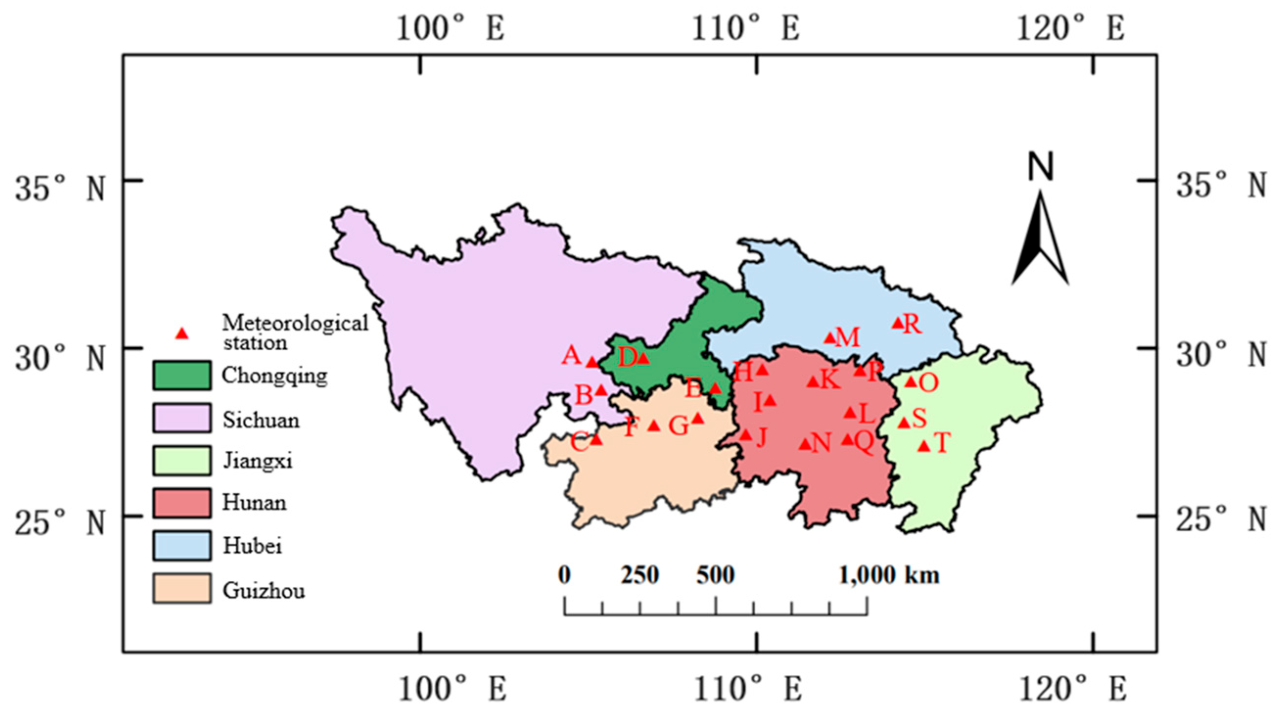
Complete meteorological data for temperature (TEMP), visibility (VISIB), wind speed (WDSP), and maximum wind speed (MXSPD) were selected from 20 meteorological stations across Sichuan Province, Guizhou Province, Chongqing Municipality, Hunan Province, Hubei Province, and Jiangxi Province, covering the period from 1 June 2024 to 31 August 2024. The 20 stations are denoted by the abbreviations A, B, C, D, E, F, G, H, I, J, K, L, M, N, O, P, Q, R, S, and T respectively. Their specific locations are illustrated in Figure 9. This map is based on the standard map with review number GS(2024)0650, sourced from the National Geographic Information Public Service Platform (Tianditu), with no modifications made to the base map.

Temperature (TEMP), visibility (VISIB), wind speed (WDSP), and maximum wind speed (MXSPD) may be regarded as four views describing meteorological conditions. Figure 10 illustrates the daily variation in these four meteorological indicators. Among them, the red curves represent the time series of each meteorological indicator, and the black curve denotes their average value. As evident from Figure 10, these indicators exhibit distinct functional characteristics, with their variations following certain patterns.

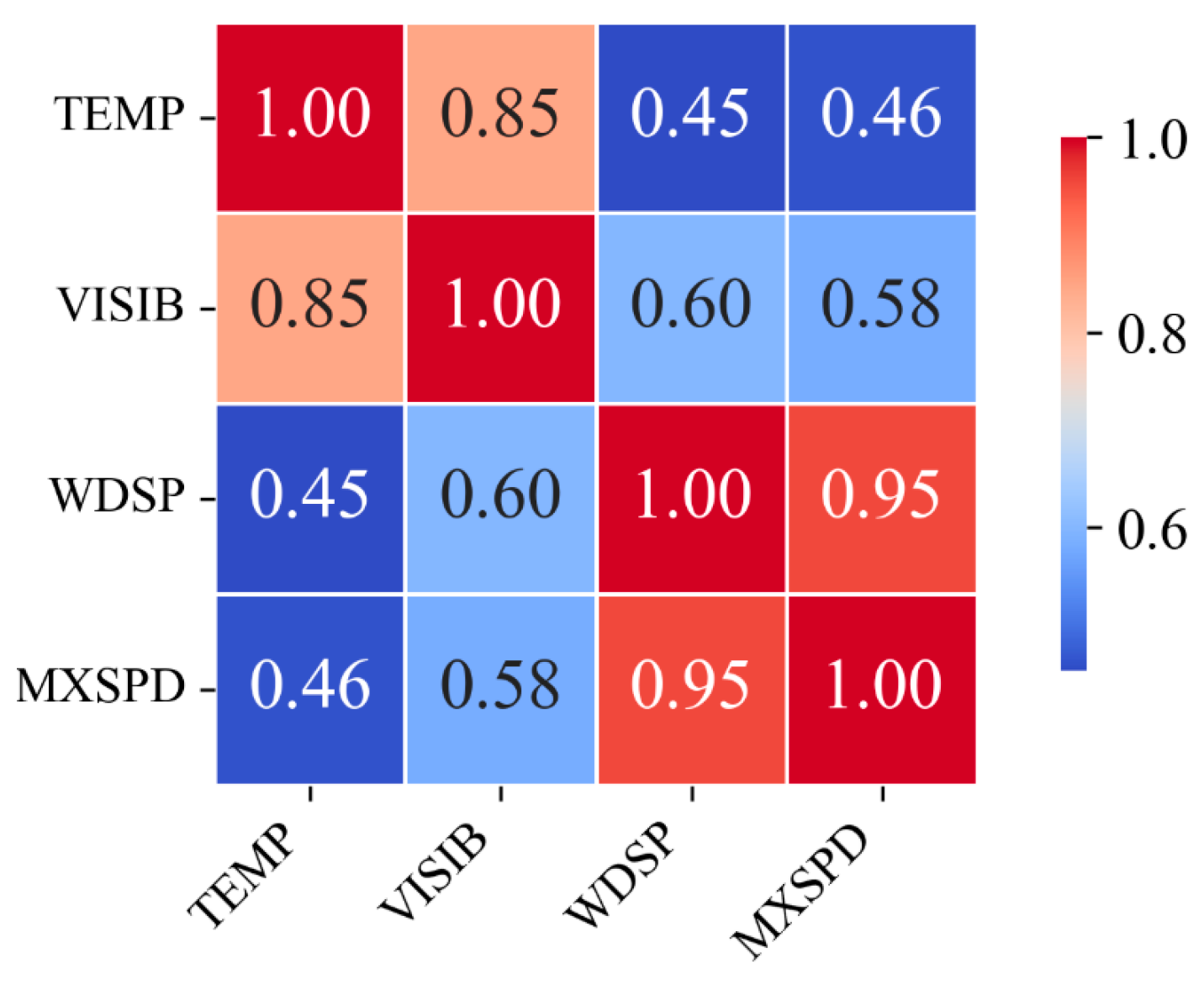
To analyze the correlation between various meteorological indicators, their Pearson correlation coefficients were calculated. The closer the absolute value of this coefficient approaches 1, the stronger the correlation between the variables. Observation of Figure 11 reveals that the correlation coefficient between WDSP and MXSPD is 0.95; that between TEMP and VISIB is 0.85; and that all four meteorological indicators exhibit positive correlations. Given the correlations among these four indicators, it is reasonable to employ their complementary characteristics for interpolating missing data.

Using complete datasets as empirical data allows for the deliberate control of the proportion, type, and location of missing data, facilitating comparative performance assessments of different imputation methods under varying conditions. Furthermore, employing complete datasets with known true values enables the precise calculation of imputation accuracy, providing a more comprehensive evaluation that facilitates objective comparisons of different methods’ performance.

Table 2. Statistical description of four meteorological index data.

Variable	Mean	SD	Max	Min	25th %Percentile	Median	75th %Percentile	Number
TEMP (°F)	55.12	2.47	60.11	49.10	53.55	55.36	57.15	1840
VISIB (mile)	16.72	2.16	18.60	8.60	15.80	17.30	18.60	1840
WDSP (knots)	4.50	0.55	6.06	3.50	4.09	4.43	4.76	1840
MXSPD (knots)	8.59	1.11	11.99	6.34	7.98	8.49	9.05	1840

presents the statistical description of the selected meteorological data.

5.2. Ablation Experiment

We artificially generate missing entries in meteorological data using a hybrid PM/IM missing data model, with specified missing rates of 20%, 30%, 40%, and 50%.

The role of the diversity constraint and adaptive graph in the objective function Equation (11) is validated through ablation experiments. Two special cases of the DCAGMFMC method are considered: eliminating the effect of the adaptive graph yields algorithm DCAGMFMC1; eliminating the effect of the diversity constraint yields algorithm DCAGMFMC2.

When the missing rate is 20%, 30%, 40%, and 50%, the RMSE and MAE of the DCAGMFMC method, DCAGMFMC1 method, and DCAGMFMC2 method are shown in

Table 3. RMSE and MAE results of four meteorological indicators under different missing rates (Mean ± Standard Deviation of 50 Results).

Missing Rate (%)	Imputation Methods	Evaluation Metric	TEMP (°C)	VISIB (Mile)	WDSP (Knots)	MXSPD (Knots)
20	DCAGMFMC	RMSE	1.55 ± 0.0283	1.47 ± 0.0224	0.70 ± 0.0214	1.16 ± 0.0232
		MAE	0.63 ± 0.0104	0.56 ± 0.0105	0.25 ± 0.0061	0.44 ± 0.0058
	DCAGMFMC1	RMSE	2.06 ± 0.0254	1.58 ± 0.0233	0.73 ± 0.0161	1.24 ± 0.0232
		MAE	0.89 ± 0.0080	0.61 ± 0.0112	0.26 ± 0.0048	0.47 ± 0.0070
	DCAGMFMC2	RMSE	2.08 ± 0.0262	1.57 ± 0.0261	0.74 ± 0.0147	1.25 ± 0.0208
		MAE	0.90 ± 0.0078	0.61 ± 0.0121	0.26 ± 0.0051	0.47 ± 0.0053
30	DCAGMFMC	RMSE	1.28 ± 0.0287	1.21 ± 0.0229	0.57 ± 0.0170	0.97 ± 0.0187
		MAE	0.43 ± 0.0092	0.38 ± 0.0085	0.16 ± 0.0042	0.30 ± 0.0041
	DCAGMFMC1	RMSE	1.70 ± 0.0234	1.27 ± 0.0186	0.62 ± 0.0175	1.01 ± 0.0151
		MAE	0.60 ± 0.0057	0.40 ± 0.0071	0.18 ± 0.0039	0.31 ± 0.0038
	DCAGMFMC2	RMSE	1.71 ± 0.0218	1.29 ± 0.0202	0.60 ± 0.0109	1.01 ± 0.0156
		MAE	0.61 ± 0.0058	0.41 ± 0.0069	0.17 ± 0.0031	0.31 ± 0.0038
40	DCAGMFMC	RMSE	1.12 ± 0.0261	1.05 ± 0.0187	0.52 ± 0.0093	0.86 ± 0.0200
		MAE	0.32 ± 0.0068	0.28 ± 0.0055	0.13 ± 0.0022	0.22 ± 0.0038
	DCAGMFMC1	RMSE	1.47 ± 0.0190	1.14 ± 0.0200	0.57 ± 0.0148	0.89 ± 0.0186
		MAE	0.45 ± 0.0045	0.31 ± 0.0065	0.13 ± 0.0025	0.24 ± 0.0032
	DCAGMFMC2	RMSE	1.48 ± 0.0221	1.14 ± 0.0157	0.54 ± 0.0128	0.88 ± 0.0145
		MAE	0.45 ± 0.0052	0.31 ± 0.0050	0.13 ± 0.0030	0.23 ± 0.0032
50	DCAGMFMC	RMSE	0.99 ± 0.0256	0.94 ± 0.0162	0.46 ± 0.0104	0.77 ± 0.0185
		MAE	0.26 ± 0.0059	0.23 ± 0.0043	0.10 ± 0.0021	0.18 ± 0.0028
	DCAGMFMC1	RMSE	1.35 ± 0.0197	1.02 ± 0.0196	0.49 ± 0.0136	0.80 ± 0.0132
		MAE	0.37 ± 0.0044	0.25 ± 0.0042	0.11 ± 0.0021	0.19 ± 0.0024
	DCAGMFMC2	RMSE	1.31 ± 0.0209	1.03 ± 0.0183	0.49 ± 0.0141	0.80 ± 0.0146
		MAE	0.36 ± 0.0040	0.25 ± 0.0051	0.11 ± 0.0022	0.19 ± 0.0023

Note: Bold text indicates superior results.

, with bold text indicating superior comparative results. Observation of Table 3 reveals that, across varying missing data rates, the DCAGMFMC method consistently exhibits lower RMSE values than both the DCAGMFMC1 and DCAGMFMC2 methods. with RMSE values consistently lower than those of DCAGMFMC1 and DCAGMFMC2. Across the four meteorological indicators, RMSE reductions ranged from 10.36% to 11.10% and 9.55% to 11.12%, respectively. This demonstrates that both diversity constraints and adaptive graphs contribute to enhancing imputation accuracy.

5.3. Application Effect and Analysis

An empirical application was conducted using complete meteorological indicator data to validate the practical effectiveness of the DCAGMFMC method. The DCAGMFMC method was employed to interpolate missing data, with root mean square error, mean absolute error, and normalized root mean square error selected as metrics to assess deviations between predicted values and actual observations. Comparisons were made against KNN, HFI, SFI, MVNFMC, and GRMFMC methods. In Equation (11), ${\theta }_v=0.8$, ${\theta }_{vs}=0.8$, $\mu =100,\lambda =1000$. The RMSE, MAE, and NRMSE results for the six imputation methods at 20%, 30%, 40%, and 50% missing data rates are presented in

Table 4. RMSE between the real data and predicted values of meteorological indicators (mean ± standard deviation of 50 results).

Missing Rate (%)	Imputation Methods	TEMP (°C)	VISIB (Mile)	WDSP (Knots)	MXSPD (Knots)
		RMSE	RMSE	RMSE	RMSE
20	KNN	2.09 ± 0.1072	3.22 ± 0.1709	2.04 ± 0.2539	3.12 ± 0.2267
	HFI	2.13 ± 0.0015	2.93 ± 0.0019	1.49 ± 0.0026	2.41 ± 0.0012
	SFI	2.14 ± 0.0011	2.92 ± 0.0008	1.49 ± 0.0019	2.43 ± 0.0022
	MVNFMC	3.63 ± 0.0155	1.99 ± 0.0237	0.90 ± 0.0134	1.47 ± 0.0245
	GRMFMC	5.89 ± 0.3016	2.73 ± 0.2030	1.55 ± 0.0704	2.37 ± 0.2344
	DCAGMFMC	1.55 ± 0.0283	1.47 ± 0.0224	0.70 ± 0.0214	1.16 ± 0.0232
30	KNN	2.37 ± 0.1349	3.42 ± 0.1474	2.10 ± 0.2538	3.26 ± 0.1969
	HFI	2.14 ± 0.0042	2.94 ± 0.0025	1.52 ± 0.0045	2.42 ± 0.0046
	SFI	2.14 ± 0.0026	2.94 ± 0.0009	1.51 ± 0.0030	2.43 ± 0.0038
	MVNFMC	2.98 ± 0.0145	1.64 ± 0.0178	0.77 ± 0.0138	1.22 ± 0.0205
	GRMFMC	4.31 ± 0.3372	2.34 ± 0.2533	1.29 ± 0.0660	1.81 ± 0.0898
	DCAGMFMC	1.28 ± 0.0287	1.21 ± 0.0229	0.57 ± 0.0170	0.97 ± 0.0187
40	KNN	2.68 ± 0.1373	3.63 ± 0.1162	2.24 ± 0.1837	3.40 ± 0.1933
	HFI	2.17 ± 0.0038	3.01 ± 0.0305	1.51 ± 0.0040	2.46 ± 0.0083
	SFI	2.18 ± 0.0060	2.97 ± 0.0079	1.52 ± 0.0030	2.43 ± 0.0040
	MVNFMC	2.56 ± 0.0171	1.39 ± 0.0158	0.65 ± 0.0072	1.08 ± 0.0156
	GRMFMC	3.15 ± 1.7703	1.51 ± 0.8450	0.83 ± 0.4679	1.22 ± 0.6879
	DCAGMFMC	1.12 ± 0.0261	1.05 ± 0.0187	0.52 ± 0.0093	0.86 ± 0.0200
50	KNN	3.02 ± 0.1289	3.84 ± 0.1447	2.27 ± 0.1432	3.40 ± 0.129
	HFI	2.23 ± 0.0192	3.03 ± 0.0272	1.53 ± 0.0089	2.47 ± 0.0100
	SFI	2.26 ± 0.0210	3.12 ± 0.0336	1.52 ± 0.0026	2.45 ± 0.0077
	MVNFMC	2.31 ± 0.0194	1.25 ± 0.0134	0.60 ± 0.0081	0.97 ± 0.0180
	GRMFMC	2.07 ± 1.8918	1.01 ± 0.9279	0.59 ± 0.5377	0.83 ± 0.7606
	DCAGMFMC	0.99 ± 0.0256	0.94 ± 0.0162	0.46 ± 0.0104	0.77 ± 0.0185

Note: Bold text indicates superior results.

,

Table 5. Mean Absolute Error (MAE) between the real data and predicted values of meteorological indicators (mean ± standard deviation of 50 results).

Missing Rate (%)	Imputation Methods	TEMP (°C)	VISIB (Mile)	WDSP (Knots)	MXSPD (Knots)
		MAE	MAE	MAE	MAE
20	KNN	1.55 ± 0.0742	2.28 ± 0.1188	1.18 ± 0.0916	2.04 ± 0.1235
	HFI	1.71 ± 0.0015	2.19 ± 0.0041	0.96 ± 0.0019	1.71 ± 0.0006
	SFI	1.71 ± 0.0019	2.17 ± 0.0029	0.95 ± 0.0024	1.72 ± 0.0008
	MVNFMC	1.70 ± 0.0067	0.80 ± 0.0087	0.33 ± 0.0035	0.58 ± 0.0064
	GRMFMC	2.53 ± 0.1387	1.09 ± 0.0865	0.54 ± 0.0258	0.83 ± 0.0833
	DCAGMFMC	0.63 ± 0.0104	0.56 ± 0.0105	0.25 ± 0.0061	0.44 ± 0.0058
30	KNN	1.76 ± 0.0910	2.45 ± 0.1085	1.23 ± 0.0812	2.12 ± 0.0963
	HFI	1.71 ± 0.0014	2.18 ± 0.0035	0.96 ± 0.0023	1.72 ± 0.0013
	SFI	1.71 ± 0.0017	2.20 ± 0.0037	0.96 ± 0.0013	1.73 ± 0.0020
	MVNFMC	1.14 ± 0.0048	0.54 ± 0.0047	0.22 ± 0.0028	0.38 ± 0.0043
	GRMFMC	1.47 ± 0.1213	0.76 ± 0.0823	0.36 ± 0.0201	0.53 ± 0.0329
	DCAGMFMC	0.43 ± 0.0092	0.38 ± 0.0085	0.16 ± 0.0042	0.30 ± 0.0041
40	KNN	1.99 ± 0.0930	2.62 ± 0.0820	1.30 ± 0.0601	2.21 ± 0.0881
	HFI	1.75 ± 0.0013	2.23 ± 0.0093	0.97 ± 0.0030	1.76 ± 0.0069
	SFI	1.73 ± 0.0013	2.18 ± 0.0031	0.97 ± 0.0029	1.73 ± 0.0011
	MVNFMC	0.84 ± 0.0050	0.40 ± 0.0037	0.17 ± 0.0016	0.29 ± 0.0028
	GRMFMC	0.93 ± 0.5280	0.42 ± 0.2368	0.20 ± 0.1144	0.32 ± 0.1770
	DCAGMFMC	0.32 ± 0.0068	0.28 ± 0.0055	0.13 ± 0.0022	0.22 ± 0.0038
50	KNN	2.24 ± 0.0984	2.78 ± 0.1089	1.34 ± 0.0489	2.24 ± 0.0642
	HFI	1.75 ± 0.0083	2.24 ± 0.0016	0.98 ± 0.0038	1.76 ± 0.0047
	SFI	1.78 ± 0.0067	2.22 ± 0.0068	0.98 ± 0.0023	1.76 ± 0.0031
	MVNFMC	0.68 ± 0.0054	0.32 ± 0.0031	0.13 ± 0.0016	0.24 ± 0.0029
	GRMFMC	0.55 ± 0.5017	0.25 ± 0.2330	0.13 ± 0.1204	0.19 ± 0.1737
	DCAGMFMC	0.26 ± 0.0059	0.23 ± 0.0043	0.10 ± 0.0021	0.18 ± 0.0028

Note: Bold text indicates superior results.

and

Table 6. NRMSE between observed and predicted values of meteorological indicators (mean ± standard deviation of 50 results).

Missing Rate (%)	Imputation Methods	TEMP (°C)	VISIB (Mile)	WDSP (Knots)	MXSPD (Knots)
		NRMSE	NRMSE	NRMSE	NRMSE
20	KNN	0.50 ± 0.0258	0.67 ± 0.0355	0.68 ± 0.0845	0.73 ± 0.0530
	HFI	0.09 ± 0.0001	0.16 ± 0.0001	0.05 ± 0.0001	0.07 ± 0.0000
	SFI	0.09 ± 0.0000	0.16 ± 0.0000	0.05 ± 0.0001	0.07 ± 0.0001
	MVNFMC	0.16 ± 0.0007	0.11 ± 0.0013	0.03 ± 0.0005	0.04 ± 0.0007
	GRMFMC	0.26 ± 0.0131	0.15 ± 0.0109	0.05 ± 0.0024	0.07 ± 0.0067
	DCAGMFMC	0.08 ± 0.0012	0.08 ± 0.0012	0.02 ± 0.0007	0.03 ± 0.0007
30	KNN	0.57 ± 0.0325	0.71 ± 0.0306	0.70 ± 0.0844	0.76 ± 0.0460
	HFI	0.09 ± 0.0002	0.16 ± 0.0001	0.05 ± 0.0002	0.07 ± 0.0001
	SFI	0.09 ± 0.0001	0.16 ± 0.0000	0.05 ± 0.0001	0.07 ± 0.0001
	MVNFMC	0.13 ± 0.0006	0.09 ± 0.0010	0.03 ± 0.0005	0.03 ± 0.0006
	GRMFMC	0.19 ± 0.0147	0.13 ± 0.0136	0.04 ± 0.0023	0.05 ± 0.0026
	DCAGMFMC	0.06 ± 0.0012	0.07 ± 0.0012	0.02 ± 0.0006	0.03 ± 0.0005
40	KNN	0.65 ± 0.0331	0.75 ± 0.0241	0.75 ± 0.0611	0.79 ± 0.0452
	HFI	0.09 ± 0.0002	0.16 ± 0.0016	0.05 ± 0.0001	0.07 ± 0.0002
	SFI	0.09 ± 0.0003	0.16 ± 0.0004	0.05 ± 0.0001	0.07 ± 0.0001
	MVNFMC	0.11 ± 0.0007	0.07 ± 0.0009	0.02 ± 0.0002	0.03 ± 0.0004
	GRMFMC	0.14 ± 0.0770	0.08 ± 0.0454	0.03 ± 0.0162	0.03 ± 0.0197
	DCAGMFMC	0.05 ± 0.0011	0.06 ± 0.0010	0.02 ± 0.0003	0.02 ± 0.0006
50	KNN	0.73 ± 0.0311	0.80 ± 0.0300	0.76 ± 0.0476	0.79 ± 0.0301
	HFI	0.10 ± 0.0014	0.16 ± 0.0007	0.05 ± 0.0001	0.07 ± 0.0002
	SFI	0.10 ± 0.0009	0.17 ± 0.0018	0.05 ± 0.0001	0.07 ± 0.0002
	MVNFMC	0.10 ± 0.0008	0.07 ± 0.0007	0.02 ± 0.0003	0.03 ± 0.0005
	GRMFMC	0.09 ± 0.0823	0.05 ± 0.0499	0.02 ± 0.0186	0.02 ± 0.0217
	DCAGMFMC	0.04 ± 0.0011	0.05 ± 0.0009	0.02 ± 0.0004	0.02 ± 0.0005

Note: Bold text indicates superior results.

, respectively, with bold text indicating superior comparative performance.

During the experiments, it was observed that the proposed method becomes unsuitable when the missing rate reaches 60%. As demonstrated in Table 4, Table 5 and Table 6, under various missing rate conditions within the experimental setup, the DCAGMFMC method consistently yields lower imputation metrics including RMSE, MAE, and NRMSE compared to KNN, HFI, SFI, MVNFMC, and GRMFMC.

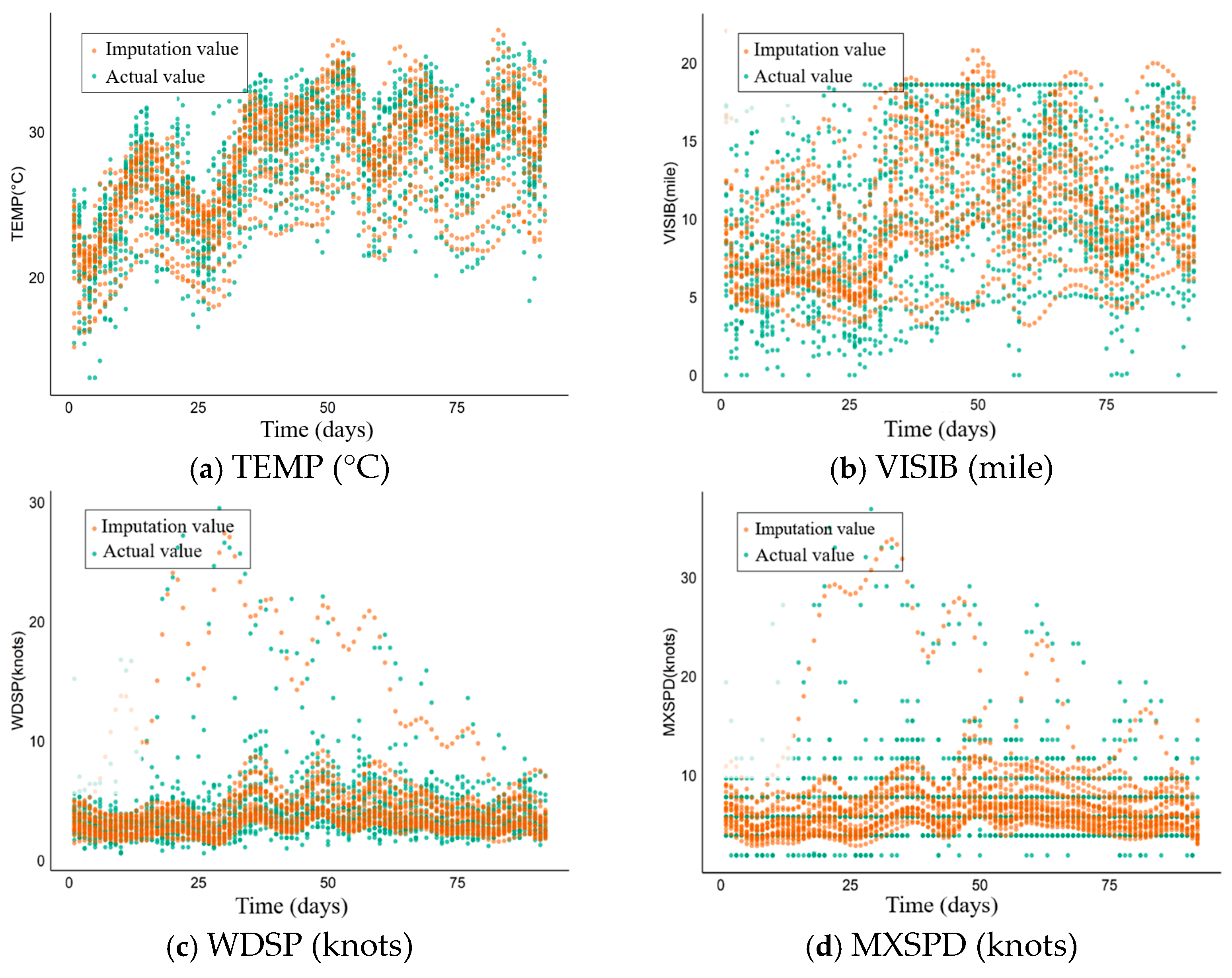
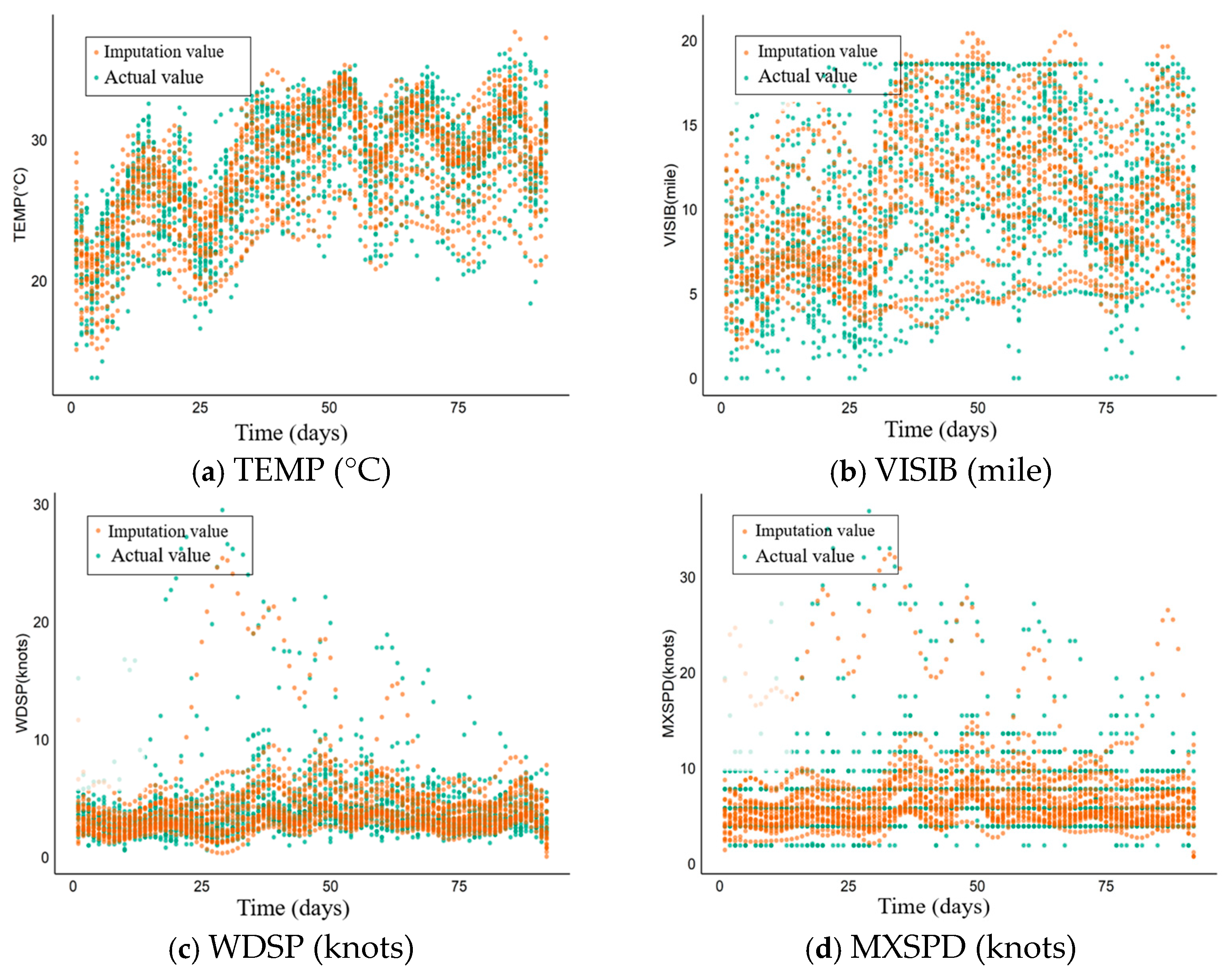
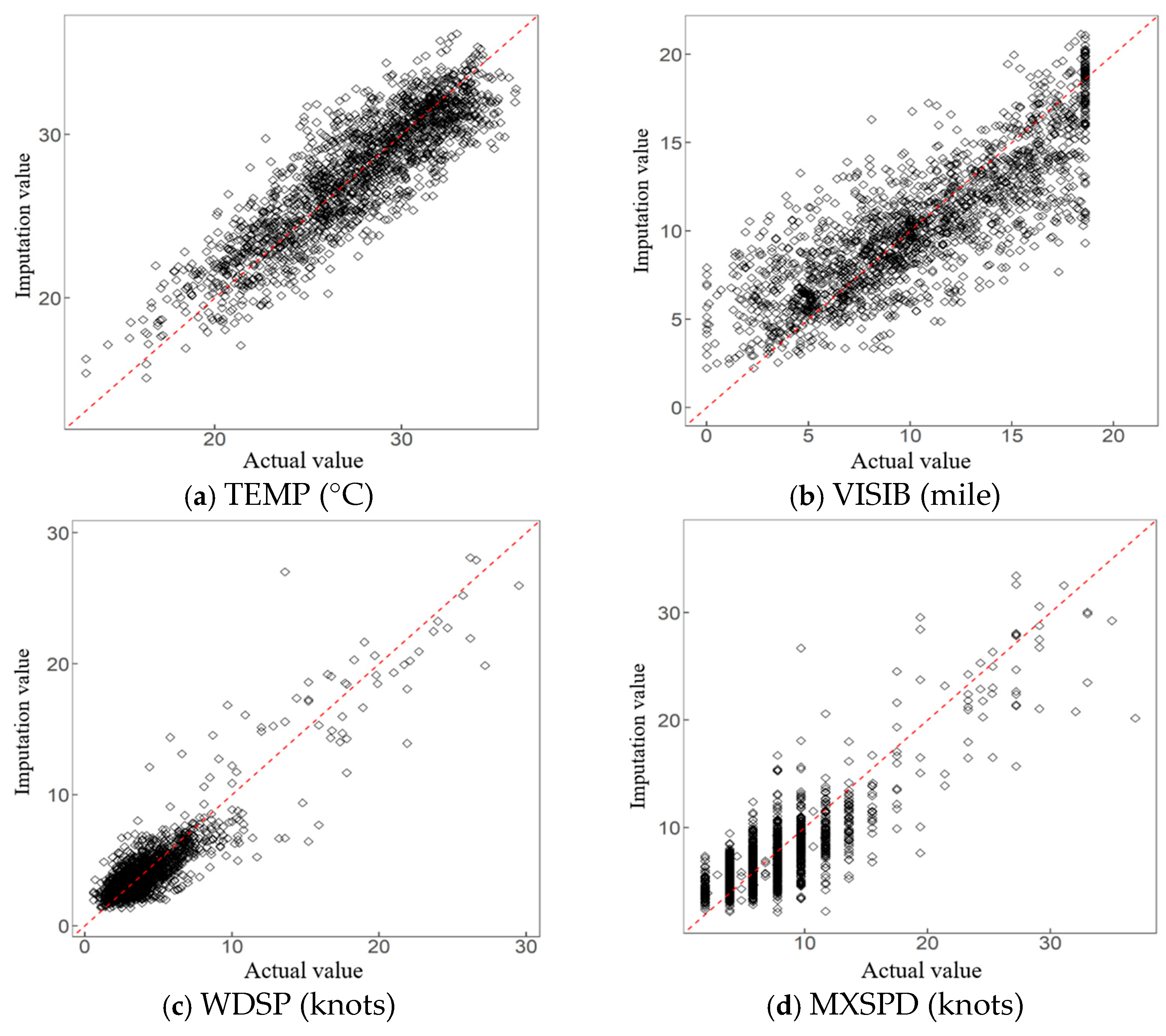
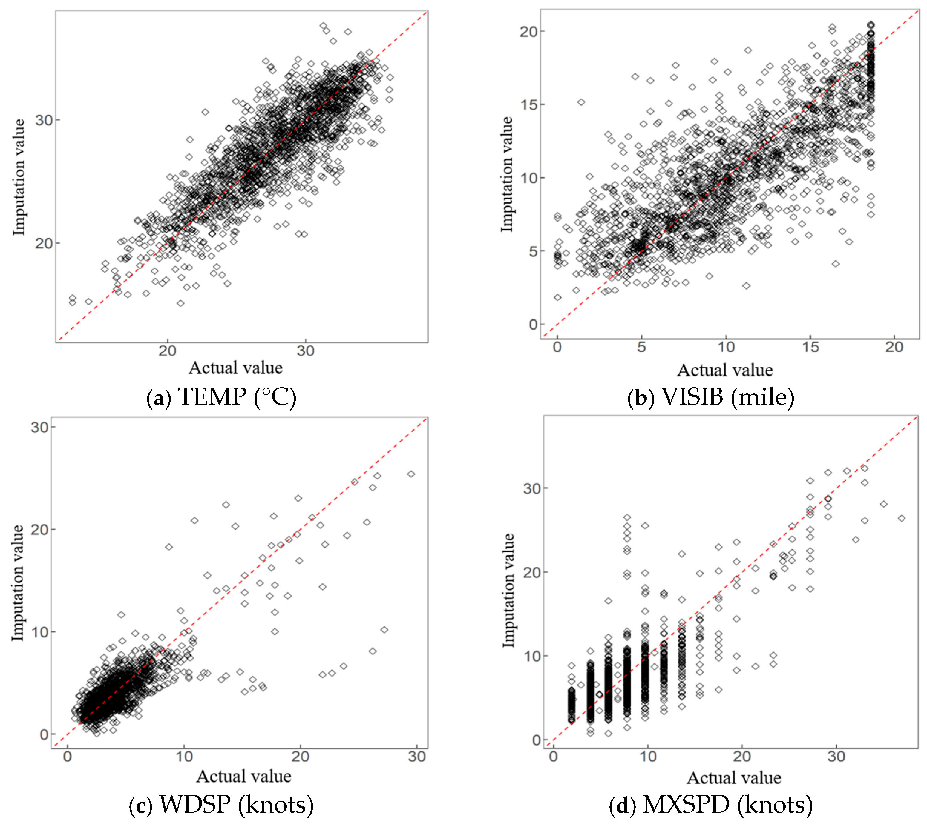
To further demonstrate the validity of the DCAGMFMC method’s interpolated values, scatter plots were plotted for the four viewpoint interpolated values against the true values at 20% and 50% missing data rates, respectively. The results are shown in Figure 12, Figure 13, Figure 14 and Figure 15. Among them, the black diamonds represent the data points of true versus imputed values, and the red dashed line denotes the 1:1 ideal fit line ($y=x$).

Figure 12 and Figure 13 demonstrate that the interpolated values exhibit good agreement with the true values at 20% and 50% missing data rates. This indicates that the DCAGMFMC method delivers satisfactory imputation results, with performance remaining stable even as the missing data rate increases. Consequently, the DCAGMFMC method is suitable for interpolating meteorological data with extensive missing values. Figure 14 and Figure 15 demonstrate that, at 20% and 50% missing data rates, the interpolated values are uniformly distributed along the 45-degree line relative to the true values. This indicates minimal error between interpolated and true values, confirming the high predictive accuracy of the DCAGMFMC method.

6. Conclusions

This study proposes a Diversity Constraint and Adaptive Graph Multi-View Functional Matrix Completion method (DCAGMFMC) within the functional data analysis framework, integrating multi-view learning with diversity constraints and adaptive graph regularization strategies. During missing value handling, the diversity constraint term accounts for inter-data variability, enhancing information utilization. The adaptive graph regularization term preserves the inherent geometric structure of the data while adaptively learning similarity matrices by maximizing their entropy. This approach enhances imputation accuracy whilst preventing model overfitting. Random simulation experiments demonstrate that the DCAGMFMC method exhibits significant imputation advantages over classical methods such as KNN, HFI, SFI, MVNFMC, and GRMFMC. Moreover, practical applications on real meteorological datasets demonstrate that the proposed method can adaptively capture dynamic correlations among multi-view observational data while preserving the intrinsic manifold structure of functional data, thereby substantially enhancing the accuracy and robustness of missing data imputation. Specifically, compared to the KNN, HFI, SFI, MVNFMC, and GRMFMC imputation methods, at different missing rates, the DCAGMFMC method achieved average RMSE reductions of 52.18–74.96%, 45.49–65.84%, 45.63–66.09%, 30.27–32.43%, and 21.97–56.43% when processing meteorological data. MAE was reduced by an average of 73.01% to 91.16%, 71.36% to 88.61%, 71.36% to 88.65%, 34.49% to 35.33%, and 22.27% to 56.10%, respectively; The NRMSE was reduced by an average of 91.25–95.78%, 44.56–65.05%, 44.56–65.51%, 25.54–33.90%, and 13.89–58.26%, respectively. Compared to these baseline methods, the DCAGMVNFMC approach achieved average reductions in RMSE, MAE, and NRMSE of 39.11–59.15%, 54.50–71.97%, and 43.96–63.70%, respectively. It also demonstrated stable interpolation performance across varying meteorological indicators and data missing rates, exhibiting strong adaptability.

The experiments in this study primarily focus on the mixed pointwise missing (PM) and interval missing (IM) patterns. However, we acknowledge that real-world missing data, particularly non-randomly absent (MNAR) data, exhibit more complex mechanisms—for instance, the probability of missingness may be correlated with the unobserved values themselves. Exploring model performance under MNAR mechanisms represents a key direction for our future work. Nevertheless, successfully handling complex interval missing (IM) data already demands robust inference and reconstruction capabilities from models, providing positive evidence for the applicability of this approach in more practical scenarios. In subsequent research, we will continue exploring novel multi-perspective functional matrix completion methods, with a focus on enhancing their interpolation performance. While fully considering the complementary information across perspectives, we strive to reduce redundancy and improve information utilization. Therefore, future research will prioritize integrating the HSIC criterion with dual-information graph strategies into the multi-perspective functional matrix completion framework. Additionally, we will explore applying the proposed DCAGMFMC method to broader practical scenarios, such as medical data interpolation and financial data interpolation.

References

1. Miao, X.; Wu, Y.; Chen, L.; Gao, Y.; Yin, J. An experimental survey of missing data Imputation algorithms. IEEE Trans. Knowl. Data Eng. 2022, 35, 6630–6650. [Google Scholar] [CrossRef]
2. Kong, X.; Zhou, W.; Shen, G.; Zhang, W.; Liu, N.; Yang, Y. Dynamic graph convolutional recurrent imputation network for spatiotemporal traffic missing data. Knowl.-Based Syst. 2023, 261, 110188. [Google Scholar] [CrossRef]
3. Gao, H.Y.; Li, W.X. Function-based multiple imputation method based on cross-sectional and longitudinal information. Tongji Yu Juece/Stat. Decis. 2025, 41, 37–42. [Google Scholar] [CrossRef]
4. Bertsimas, D.; Pawlowski, C.; Zhuo, Y.D. From predictive methods to missing data imputation: An optimization approach. J. Mach. Learn. Res. 2018, 18, 1–39. Available online: https://jmlr.org/papers/v18/17-073.html (accessed on 15 October 2024).
5. Yao, F.; Müller, H.G.; Wang, J.L. Functional data analysis for sparse longitudinal data. J. Am. Stat. Assoc. 2005, 100, 577–590. [Google Scholar] [CrossRef]
6. Royston, P.; White, I.R. Multiple Imputation by Chained Equations (MICE): Implementation in Stata. J. Stat. Softw. 2011, 45, 1–20. [Google Scholar] [CrossRef]
7. He, Y.; Yucel, R.; Raghunathan, T.E. A functional multiple imputation approach to incomplete longitudinal Data. Stat. Med. 2011, 30, 1137–1156. [Google Scholar] [CrossRef]
8. Ciarleglio, A.; Petkova, E.; Harel, O. Elucidating age and sex-dependent association between frontal EEG asymmetry and depression: An application of multiple imputation in functional regression. J. Am. Stat. Assoc. 2022, 117, 12–26. [Google Scholar] [CrossRef]
9. Rao, A.R.; Reimherr, M. Modern multiple imputation with functional data. Stat 2021, 10, e331. [Google Scholar] [CrossRef]
10. Li, J.W.; Sun, Y.H.; Wang, S.; Zhang, Z.W.; Wang, Y. Ultra-short-term load forecasting considering missing data in abnormal situations. Autom. Electr. Power Syst. 2025, 49, 133–143. [Google Scholar] [CrossRef]
11. Liu, Y.; Zhao, Y.P.; Liu, F.Q.; Kong, X.F.; Ma, R. Research progress on abnormal and missing data processing methods in marine environmental monitoring. J. Appl. Oceanogr. 2025, 44, 388–401. [Google Scholar] [CrossRef]
12. Liang, Y.P.; Li, X.Y.; Li, Q.G.; Mao, S.R.; Zhen, M.H.; Li, J.B. Research on intelligent prediction of gas concentration in working face based on CS-LSTM. J. Mine Saf. Environ. Prot. 2022, 49, 80–86. [Google Scholar] [CrossRef]
13. Wu, Y.H.; Wang, Y.S.; Xu, H.; Chen, Z.; Zhang, Z.; Guan, S.J. Review on wind power output prediction technology. Comput. Sci. Explor. 2022, 16, 2653–2677. [Google Scholar] [CrossRef]
14. Kidzinski, Ł.; Hastie, T. Longitudinal data analysis using matrix completion. Stat 2018, 1050, 24. [Google Scholar] [CrossRef]
15. Xue, J.; Fu, D.Y.; Han, H.B.; Gao, H.Y. A non-negative functional matrix completion algorithm based on multi-view learning. Stat. Decis. 2022, 38, 5–11. [Google Scholar] [CrossRef]
16. Kramer, O. K-nearest neighbors. In Dimensionality Reduction with Unsupervised Nearest Neighbors; Springer: Berlin/Heidelberg, Germany, 2013; pp. 13–23. [Google Scholar] [CrossRef]
17. Gao, H.Y.; Liu, C.; Ma, W.J. Comparison and application of time series data imputation methods for surface water quality monitoring. Hydrology 2024, 44, 63–69. [Google Scholar] [CrossRef]
18. Nelwamondo, F.V.; Mohamed, S.; Marwala, T. Missing data: A comparison of neural network and expectation maximization techniques. Curr. Sci. 2007, 93, 1514–1521. Available online: https://www.jstor.org/stable/24099079 (accessed on 15 October 2024).
19. Koren, Y.; Bell, R.; Volinsky, C. Matrix factorization techniques for recommender systems. Computer 2009, 42, 30–37. [Google Scholar] [CrossRef]
20. Yu, H.F.; Rao, N.; Dhillon, I.S. Temporal regularized matrix factorization for high-dimensional time series prediction. Adv. Neural Inf. Process. Syst. 2016, 29. Available online: https://proceedings.neurips.cc/paper_files/paper/2016/hash/85422afb467e9456013a2a51d4dff702-Abstract.html (accessed on 24 October 2025).
21. He, J.; Lai, Z.; Shi, K. Time series imputation method based on joint tensor completion and recurrent neural network. Data Acquis. Process. 2024, 39, 598–608. [Google Scholar] [CrossRef]
22. Cao, W.; Wang, D.; Li, J.; Zhou, H.; Li, L.; Li, Y. BRITS: Bidirectional recurrent imputation for time series. Adv. Neural Inf. Process. Syst. 2018, 31. Available online: https://proceedings.neurips.cc/paper_files/paper/2018/hash/734e6bfcd358e25ac1db0a4241b95651-Abstract.html (accessed on 24 October 2025).
23. Carmona, C.U.; Aubet, F.X.; Flunkert, V.; Gasthaus, J. Neural contextual anomaly detection for time series. arXiv 2021, arXiv:2107.07702. [Google Scholar] [CrossRef]
24. Yoon, J.S.; Jordon, J.; Schaar, M. GAIN: Missing data imputation using generative adversarial nets. In Proceedings of the International Conference on Machine Learning, Stockholm, Sweden, 10–15 July 2018. [Google Scholar] [CrossRef]
25. Wang, J.L.; Chiou, J.M.; Müller, H.G. Functional data analysis. Annu. Rev. Stat. Appl. 2016, 3, 257–295. [Google Scholar] [CrossRef]
26. Ullah, S.; Finch, C.F. Applications of functional data analysis: A systematic review. BMC Med. Res. Methodol. 2013, 13, 43. [Google Scholar] [CrossRef]
27. Yao, X.H. Research on Several Multivariate Functional Clustering Methods Based on Multi-View Learning. Ph.D. Thesis, Lanzhou University of Finance and Economics, Lanzhou, China, 2022. Available online: https://library.lzufe.edu.cn/asset/detail/0/20471970033 (accessed on 24 October 2025).
28. Descary, M.H.; Panaretos, V.M. Functional data analysis by matrix completion. Ann. Stat. 2019, 47, 1–38. [Google Scholar] [CrossRef]
29. Kong, S.; Wang, X.; Wang, D.; Wu, F. Multiple feature fusion for face recognition. In Proceedings of the 2013 10th IEEE International Conference and Workshops on Automatic Face and Gesture Recognition (FG), Shanghai, China, 22–26 April 2013; pp. 1–7. [Google Scholar] [CrossRef]
30. Xu, H.; Zhang, X.; Xia, W.; Gao, Q.; Gao, X. Low-rank tensor constrained co-regularized multi-view spectral clustering. Neural Netw. 2020, 132, 245–252. [Google Scholar] [CrossRef] [PubMed]
31. Wu, K.; Xiao, Y.S.; Liu, B. Multi-view semi-supervised marked distribution learning. Comput. Appl. Res. 2025, 42, 1–8. Available online: https://www.arocmag.cn/abs/2025.04.0114 (accessed on 24 October 2025).
32. Gao, H.Y.; Ma, W.J. Air quality data restoration based on graph regularization and multi-view function matrix completion. China Environ. Sci. 2024, 44, 5357–5370. [Google Scholar] [CrossRef]
33. Li, C.; Che, H.; Leung, M.F.; Liu, C.; Yan, Z. Robust multi-view non-negative matrix factorization with adaptive graph and diversity constraints. Inf. Sci. 2023, 634, 587–607. [Google Scholar] [CrossRef]
34. Wang, J.; Tian, F.; Yu, H.; Liu, C.H.; Zhan, K.; Wang, X. Diverse non-negative matrix factorization for multiview data representation. IEEE Trans. Cybern. 2017, 48, 2620–2632. [Google Scholar] [CrossRef] [PubMed]
35. Liang, N.; Yang, Z.; Li, Z.; Sun, W.; Xie, S. Multi-view clustering by non-negative matrix factorization with co-orthogonal constraints. Knowl.-Based Syst. 2020, 194, 105582. [Google Scholar] [CrossRef]
36. Cai, D.; He, X.; Han, J.; Huang, T.S. Graph regularized nonnegative matrix factorization for data representation. IEEE Trans. Pattern Anal. Mach. Intell. 2010, 33, 1548–1560. [Google Scholar] [CrossRef] [PubMed]
37. Li, J.; Zhou, G.; Qiu, Y.; Wang, Y.; Zhang, Y.; Xie, S. Deep graph regularized non-negative matrix factorization for multi-view clustering. Neurocomputing 2020, 390, 108–116. [Google Scholar] [CrossRef]
38. Yang, X.; Che, H.; Leung, M.F.; Liu, C. Adaptive graph nonnegative matrix factorization with the self-paced regularization. Appl. Intell. 2023, 53, 15818–15835. [Google Scholar] [CrossRef]
39. Luo, P.; Peng, J.; Guan, Z.; Fan, J. Dual regularized multi-view non-negative matrix factorization for clustering. Neurocomputing 2018, 294, 1–11. [Google Scholar] [CrossRef]
40. Li, X.; Zhang, H.; Zhang, R.; Liu, Y.; Nie, F. Generalized uncorrelated regression with adaptive graph for unsupervised feature selection. IEEE Trans. Neural Netw. Learn. Syst. 2018, 30, 1587–1595. [Google Scholar] [CrossRef]
41. Hunter, D.R.; Lange, K. A tutorial on MM algorithms. Am. Stat. 2004, 58, 30–37. [Google Scholar] [CrossRef]
42. Tseng, P. Convergence of a block coordinate descent method for nondifferentiable minimization. J. Optim. Theory Appl. 2001, 109, 475–494. [Google Scholar] [CrossRef]
43. Mucherino, A.; Papajorgji, P.J.; Pardalos, P.M. K-nearest neighbor classification. In Data Mining in Agriculture; Springer: New York, NY, USA, 2009; pp. 83–106. [Google Scholar] [CrossRef]
44. Jacques, J.; Preda, C. Model-based clustering for multivariate functional data. Comput. Stat. Data Anal. 2014, 71, 92–106. [Google Scholar] [CrossRef]
45. Boor, C.D. A Practical Guide to Splines; Springer: New York, NY, USA, 1978. [Google Scholar] [CrossRef]
46. Chiou, J.M.; Zhang, Y.C.; Chen, W.H.; Chang, C.W. A functional data approach to missing value imputation and outlier detection for traffic flow data. Transp. B Transp. Dyn. 2014, 2, 106–129. [Google Scholar] [CrossRef]
47. NOAA National Centers for Environmental Information. Global Summary of the Day—Weather Data. 2024. Available online: https://www.ncei.noaa.gov/data/global-summary-of-the-day/archive (accessed on 1 October 2024).
Figure 1. Schematic diagram of the DCAGMFMC algorithm.
Axioms 14 00793 g001
Figure 2. Multi-View data generated by normal noise and exponential noise in Case a.
Axioms 14 00793 g002
Figure 3. Multi-View data generated by normal noise and exponential noise in Case b.
Axioms 14 00793 g003
Figure 4. RMSE results for different parameters μ and λ under normal noise in case a at different views.
Axioms 14 00793 g004
Figure 5. RMSE results for different parameters μ and λ under exponential noise in case a at different views.
Axioms 14 00793 g005
Figure 6. RMSE results for different parameters μ and λ under normal noise in case b at different views.
Axioms 14 00793 g006
Figure 7. RMSE results for different parameters μ and λ under exponential noise in case b at different views.
Axioms 14 00793 g007
Figure 8. Visualization of data missing situations for four meteorological indicators.
Axioms 14 00793 g008
Figure 9. Distribution map of 20 meteorological stations. (Note: The map coordinate system is WGS 1984 (EPSG:4326)).
Axioms 14 00793 g009
Figure 10. Trends in the numerical changes of four meteorological indicators.
Axioms 14 00793 g010
Figure 11. Heatmap of correlation coefficients for four meteorological indicators.
Axioms 14 00793 g011
Figure 12. Scatter plot of true values vs. imputed values under 20% missing rate.
Axioms 14 00793 g012
Figure 13. Scatter plot of true values vs. imputed values under 50% missing rate.
Axioms 14 00793 g013
Figure 14. Graph of the relationship between true values and imputation values at a 20% missing rate.
Axioms 14 00793 g014
Figure 15. Graph of the relationship between true values and imputation values at a 50% missing rate.
Axioms 14 00793 g015