The Characteristic Relation in Two-Dimensional Type I Intermittency ^†

Abstract

To explore intermittency in discrete systems with two or more degrees of freedom, we analyze the general characteristics of type I intermittency within a two-dimensional map. This investigation is carried out numerically, concentrating on the system’s attractors, bifurcation diagrams, and the characteristic relation associated with type I intermittency. We present two methods for determining the laminar interval and the channel structure. Our computations yield numerical results for the average laminar length as a function of the control parameter, which we then compare with findings from intermittency in one-dimensional maps. We observe a strong agreement between the numerical data and the theoretical predictions.

1. Introduction

Chaotic intermittency is an interesting phenomenon observed in dynamical systems, characterized by a distinctive alternation between chaotic and laminar or regular behaviors. During the laminar phases, which may also be referred to as pseudo-equilibrium regions or pseudo-periodic solutions, the solution of the system moves close to the previous stable solution. In contrast, the bursts that occur during the chaotic phases signify a transition to irregular patterns. This duality highlights the complex nature of dynamical systems and the intricate balance between regular and chaotic behavior within their evolution. Understanding these dynamics is crucial for analyzing a wide range of complex systems, whether they are of natural or human origin [1]. Intermittency is a route that leads to chaos and has been found in physics, engineering, astronomy, chemistry, medicine, neurosciences, economics, biology, and genetics [2,3,4,5,6,7,8,9,10,11,12,13,14,15,16,17,18,19,20,21,22,23]. A more detailed description of chaotic intermittency could lead to a better understanding of these phenomena. Consequently, this area of research has the potential to provide significant benefits across various fields. Additionally, accurately describing chaotic intermittency is crucial for systems that have incomplete or unknown equations.

About 45 years ago, chaotic intermittency was classified into three distinct types, referred to as I, II, and III [9,24]. This classification depends on the bifurcation that gives rise to the intermittency. This bifurcation occurs when the eigenvalues of the system’s Jacobian matrix—evaluated in the local solution—depart from the unit circle. Type I intermittency is characterized by an eigenvalue exiting the unit circle through +1, while type II involves two complex conjugated eigenvalues leaving the unit circle. Finally, type III is defined by an eigenvalue leaving the unit circle through −1 [25,26,27]. Subsequent research introduced additional types of chaotic intermittency, including on-off, eyelet, ring, in-out, type X, and type V (see [27,28] and references there).

One-dimensional maps, commonly referred to as Poincaré maps, offer an alternative for investigating chaotic intermittency. Two essential elements characterize these maps: a specific local map, which establishes the intermittency type, and a reinjection mechanism returning the trajectories from the chaotic dynamics to the regular phase. The core of this process is encapsulated in the reinjection probability density function (RPD). The RPD quantifies the probability of trajectories re-entering the laminar zone around an unstable or disappearing fixed point. When paired with the local map, the RPD function provides profound insights into the dynamical characteristics of the system. Determining the RPD function correctly is paramount for a comprehensive understanding of chaotic intermittency. However, extracting the RPD from experimental or numerical data can be quite challenging due to the vast amounts of data and the inherent statistical fluctuations. Various strategies have emerged for calculating the RPD function. Traditionally, the classical framework for chaotic intermittency has relied on the assumption of uniform reinjection within the laminar interval. Recently, two innovative methodologies have been developed to more accurately derive the RPD function. The first, the M function methodology, introduces a generalized power law for the RPD and has demonstrated remarkable accuracy for a wide range of one-dimensional maps exhibiting type I, II, III, and V intermittencies. This approach not only integrates the classical approximation but also accommodates uniform reinjection as a specific instance. The second methodology, known as the continuity technique, employs the Perron–Frobenius operator to effectively compute the reinjection probability density function. Like the M function methodology, the continuity technique has been validated across various maps displaying different types of intermittency. To gain deeper insights into the phenomenon of intermittency, it is also essential to consider other statistical functions, such as the probability density of laminar lengths, $\psi \left(l\right)$, the average laminar length, $\overline{l}$, and the characteristic relation $\overline{l}=\overline{l}\left(\epsilon \right)$. These functions, however, are contingent on the RPD. Furthermore, the RPD and the related statistical functions that characterize chaotic intermittency are influenced by external noise and the lower boundary of reinjection (LBR). Remarkably, the M function methodology has been further refined to encompass both of these crucial aspects [27,28].

However, these previous studies only consider one-dimensional maps. In this paper, we are interested in analyzing chaotic intermittency in two-dimensional maps, more specifically, we analyze the characteristic relation, the dependence of the average laminar length, $\overline{l}$, with the control parameter $\epsilon$ for type I intermittency. To carry out this task, we study a 2D map introduced in [29], which exhibits type I intermittency. The researchers provided a comprehensive description of the structure of the reinjection channel and the trajectory within it, resulting in the establishment of scaling relations based on the trajectory.

The main objective of this paper is to investigate the phenomenon of chaotic intermittency. In addition, it includes a partial analysis of specific attractors within the system. However, this study does not aim to provide a comprehensive description of the system’s attractors, and the methodology employed is not particularly well-suited for uncovering hidden chaotic attractors [30].

This study focuses on the dynamics of the system, examining the basins of attraction for different attractors, analyzing various trajectories within the channel, and calculating the exponents of the characteristic relation. The findings presented in this research serve as a preliminary exploration of the potential for extending the new theory of chaotic intermittency [27,28] to high-dimensional maps. This article is a revised and expanded version of a paper entitled “Intermitencia en un mapa bidimensional”, which was presented at XXXIX Congreso Argentino de Mecánica Computacional, Concordia, Argentina in November 2023 [31].

This paper is organized as follows: In Section 2, we introduce the two-dimensional map and analyze the dynamics of the system. We describe the fixed points and assess their stability, followed by the presentation of bifurcation diagrams along with an explanation of the attraction basins. Section 3 explores the type I intermittency observed in the two-dimensional map. We illustrate this intermittency for various values of the control parameters, which correspond to different trajectories related to 14 cycles and 10 cycles. Finally, Section 4 summarizes the main conclusions and discusses perspectives for future research.

2. Two-Dimensional System

A general map in d-dimensions can be written as

$${\overline{x}}_{n+1}=\overline{f}\left({\overline{x}}_n\right)$$

(1)

where ${\overline{x}}_n\in {\mathbf{R}}^d$ is a finite-dimensional vector, being ${\mathbf{R}}^d$ the d-dimensional Euclidean space, and d is an integer number verifying $d>1$.

In a two-dimensional vector space defined by the pair $({\overline{x}}_{n+1},{\overline{x}}_n)$, the equation ${\overline{x}}_{n+1}={\overline{x}}_n$ represents a diagonal hyper-surface (DHS) [29]. In type I intermittency, the DHS surface, along with the local map, establishes a channel that allows the system to enter a laminar phase as the trajectory passes through it. The function of the DHS surface in two-dimensional maps is similar to that of the bisector line in one-dimensional maps.

In this paper, we analyze the two-dimensional map, $d=2$, proposed by [29]:

$$\begin{array}{cc}\hfill & x_{n+1}=F\left(x_n,y_n\right)=4\alpha x_n\left(1-x_n\right)+\beta y_n\left(1-x_n\right)\hfill \\ \hfill & y_{n+1}=G\left(x_n,y_n\right)=4\alpha y_n\left(1-y_n\right)+\beta x_n\left(1-y_n\right)\hfill \end{array}$$

(2)

where $\alpha$ and $\beta$ are control parameters, and the vector ${\overline{x}}_n=(x_n,y_n)\in {\mathbf{R}}^2$.

We perform a classical analysis of the dynamics of the system for a fixed value of $\beta$. In this analysis, the dynamics are determined by the parameter $\alpha$. We calculate the fixed points and assess their stability, and we also generate bifurcation diagrams and basins of attraction for the system’s attractors.

The fixed points of the system are all pairs $(x^{*},y^{*})$ such that $x^{*}=F(x^{*},y^{*})$ and $y^{*}=G(x^{*},y^{*})$. The stability of these points is determined by the dynamic behavior in their vicinity. Some points can attract nearby trajectories, while others can repel them, and some may act as centers for periodic trajectories. The stability of fixed points can be analyzed by considering the eigenvalues of the Jacobian matrix.

$$J=\left|\begin{array}{cc}{\partial }_{x}F\left(x^{*},y^{*}\right)& {\partial }_{y}F\left(x^{*},y^{*}\right)\\ {\partial }_{x}G\left(x^{*},y^{*}\right)& {\partial }_{y}G\left(x^{*},y^{*}\right)\end{array}\right|$$

(3)

Evaluating the stability of a system’s solutions requires a comprehensive understanding of the system dynamics. The eigenvalues of the Jacobian matrix are critical in determining the stability of the fixed points, as they provide important information about the system’s response to perturbations. These eigenvalues exist within the complex plane, and a fixed point is classified as hyperbolic if no eigenvalue is located on the unit circle.

The stability condition indicates that if at least one eigenvalue lies outside the unit circle, the fixed point is unstable, whereas it is considered stable if all eigenvalues are within the unit circle. If at least one eigenvalue of the fixed point is on the unit circle, the fixed point is categorized as non-hyperbolic, for which the stability condition based on the eigenvalues of the Jacobian matrix is insufficient.

Bifurcation diagrams illustrate the behavior of dynamical systems, showing the solutions and their stability within the state-control space. In these diagrams, stable solutions are represented as stable branches, while unstable solutions are depicted as unstable branches. Generally, a branch of solutions will either commence, terminate, or change its stability at a bifurcation point [25].

Each attractor of the system, $\overline{X}$, possesses its basin or domain of attraction, which is the domain $D\in {\mathbf{R}}^d$ that includes all the initial conditions ${\overline{x}}_0$ such ${\overline{f}}^n\left({\overline{x}}_0\right)\to \overline{X}$ as $n\to \infty$.

As a first step to determine the dynamics behavior, we start with the calculation of the fixed points of the map $\overline{f}(x,y)$, given by Equations (2). The fixed points have been calculated using analytic methods. For $\beta =0.5$, they are:

$$\begin{array}{cccc}\hfill & x_1^{*}=0\hfill & \hfill & y_1^{*}=0\hfill \end{array}$$

(4)

$$\begin{array}{cccc}\hfill & x_2^{*}={\displaystyle \frac{\alpha -0.125}{\alpha +0.125}}\hfill & \hfill & y_2^{*}={\displaystyle \frac{\alpha -0.125}{\alpha +0.125}}\hfill \end{array}$$

(5)

$$\begin{array}{cccc}\hfill & x_3^{*}={\displaystyle \frac{0.09375-0.25\alpha }{0.046875+\left(-0.5+\alpha \right)\alpha +A}}\hfill & \hfill & y_3^{*}={\displaystyle \frac{0.09375-0.25\alpha }{0.046875+\left(-0.5+\alpha \right)\alpha -A}}\hfill \end{array}$$

(6)

$$\begin{array}{cccc}\hfill & x_4^{*}={\displaystyle \frac{0.09375-0.25\alpha }{0.046875+\left(-0.5+\alpha \right)\alpha -A}}\hfill & \hfill & y_4^{*}={\displaystyle \frac{0.09375-0.25\alpha }{0.046875+\left(-0.5+\alpha \right)\alpha +A}}\hfill \end{array}$$

(7)

where $A=\sqrt{\left(\alpha -0.375\right)\left(\alpha -0.125\right)\left({\alpha }^2+0.046875\right)}$.

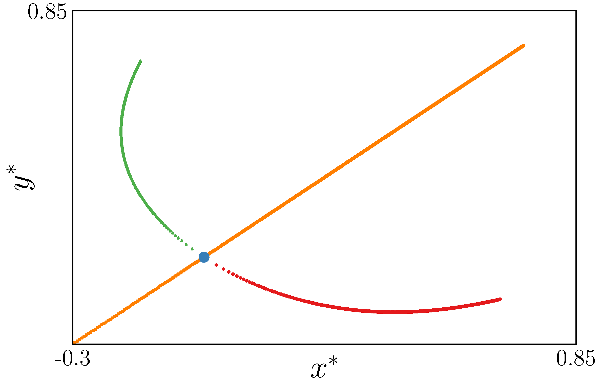
Once the control parameter $\beta$ is established, the fixed points of the system depend only on the other control parameter, $\alpha$. Figure 1 and Figure 2 show the evolution of the fixed points with $\alpha$. From the figures, we can observe that the fixed point $(x_1^{*},y_1^{*})$ does not depend on $\alpha$.

To generate a bifurcation diagram, we start by iterating the system from chosen initial values, denoted as $(x_0,y_0)$. This iterative process continues until we arrive at a solution that characterizes the system’s behavior. Once this is achieved, we repeat the iteration process using various values of the control parameter $\alpha$.

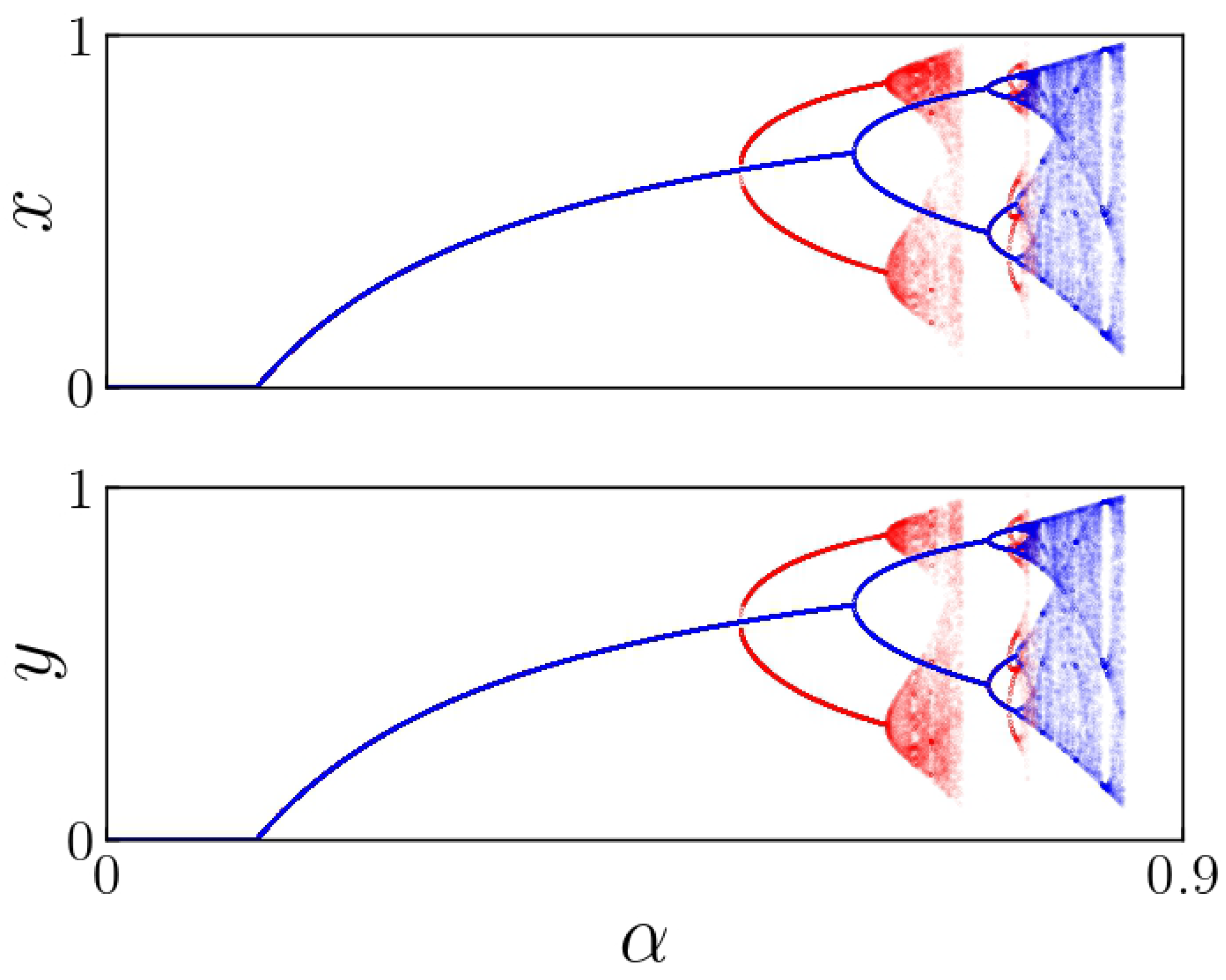
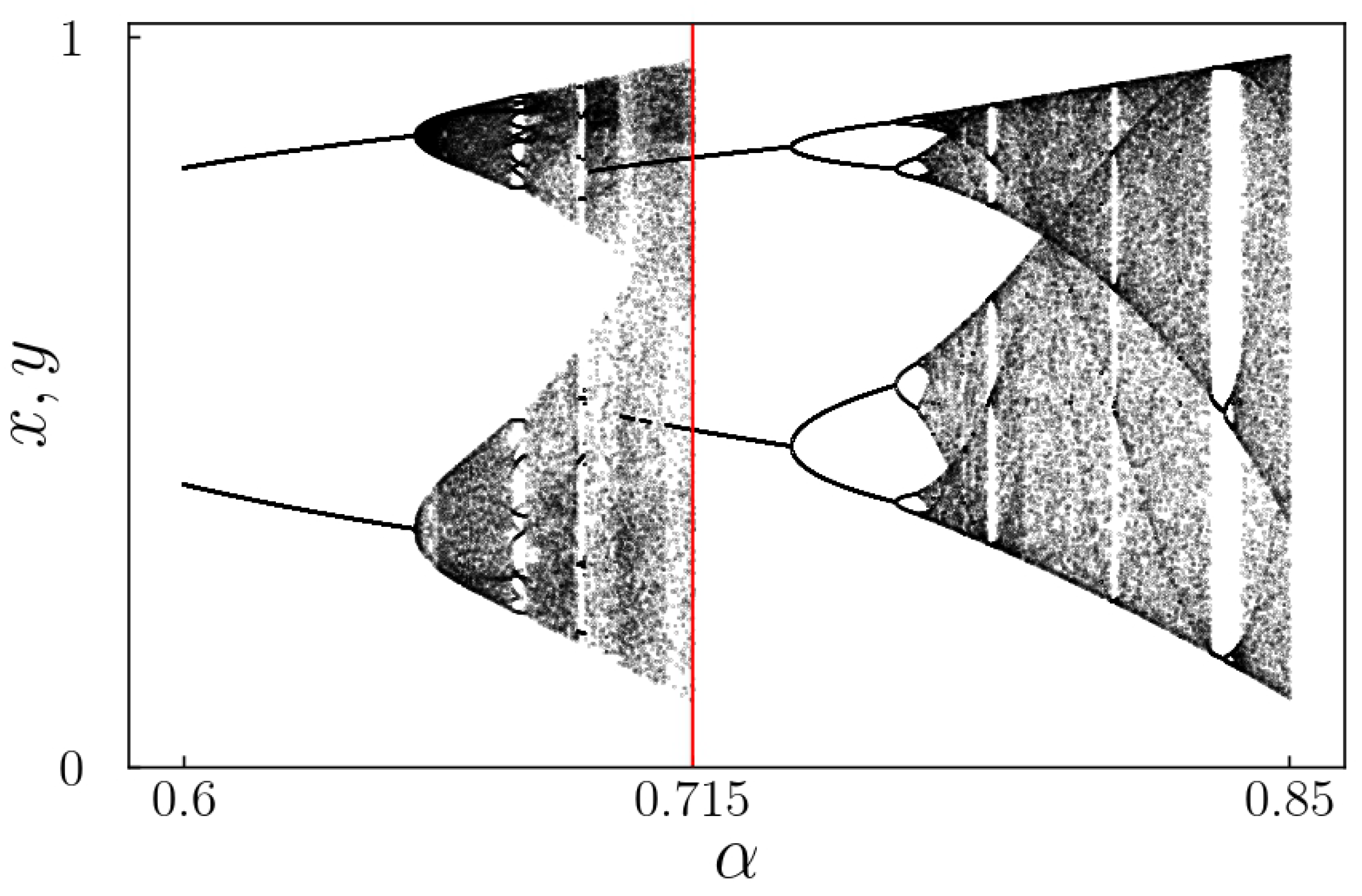
Figure 3 presents a bifurcation diagram consisting of two superimposed plots: one in blue and the other in red. The blue plot illustrates the stationary solutions derived from initial conditions where $x_0=y_0$, with each value of $\alpha$ held constant. This plot resembles a one-dimensional bifurcation diagram that follows the logistic equation, as the system described in Equations (2) is decoupled, functioning as two separate one-dimensional logistic maps.

In contrast, the red plot represents results from random initial conditions $(x_0\ne y_0$) in the interval $(0,1)$ for each value of $\alpha$. This curve exhibits its first bifurcation around $\alpha =0.53$, indicating a period-doubling bifurcation. The blue curve’s first bifurcation, however, occurs at $\alpha =0.62$, as depicted in Figure 3. Each bifurcation corresponds to an eigenvalue departing from the unit circle through $-1$, resulting in a period-doubling bifurcation. Fixed points on the upper branches are unstable, while those on the lower branches remain stable until $\alpha \approx 0.85$ for the blue plot and $\alpha \approx 0.77$ for the red diagram. Fixed points on the lower branches become unstable or vanish beyond these values of $\alpha$.

The provided figures indicate a significant correlation between the initial conditions and the observed attractors. Consequently, each bifurcation diagram exhibits distinct basins of attraction. This information will be essential for developing a comprehensive understanding of the system’s behavior and gaining insights into its dynamics.

As examples, we indicate some periodic points corresponding to different values of $\alpha$ that belong to solutions of periods 2, 4, 8, and 16, as shown in [32].

Fixing the $\beta$ parameter at $0.3$ and increasing $\alpha$, with equal initial conditions $x_0=y_0$ yields 2, 4, 8, and 16 period solutions for values of $\alpha$ 0.7, 0.79, 0.816, 0.8166.

With $\alpha =0.7$ the fixed points are $(x_1=0.55,y_1=0.558)$, $(x_2=0.764,y_2=0.764)$, with $\alpha =0.79$: $(x_1=0.467,y_1=0.467)$, $(x_2=0.861,y_2=0.861)$, $(x_3=0.413,y_3=0.413)$, $(x_4=0.838,y_4=0.838)$; for $\alpha =0.816$: $(x_1=0.346,y_2=0.346)$, $(x_2=0.807,y_2=0.807)$, $(x_3=0.553,y_3=0.553)$, $(x_4=0.880,y_4=0.880)$, $(x_5=0.374,y_5=0.374)$, $(x_6=0.835,y_6=0.835)$, $(x_7=0.490,y_7=0.490)$, $(x_8=0.890,y_8=0.890$; and finally for $\alpha =0.8166$: $(x_1=0.378,y_1=0.378)$, $(x_2=0.838,y_2=0.838)$, $(x_3=0.482,y_3=0.482)$, $(x_4=0.890,y_4=0.890)$, $(x_5=0.347,y_5=0.347)$, $(x_6=0.809,y_6=0.809)$, $(x_7=0.551,y_7=0.551)$, $(x_8=0.882,y_8=0.882)$, $(x_9=0.370,y_9=0.370)$, $(x_{10}=0.831,y_{10}=0.831)$, $(x_{11}=0.499,y_{11}=0.499)$, $(x_{12}=0.891,y_{12}=0.891)$, $(x_{13}=0.344,y_{13}=0.344)$, $(x_{14}=0.805,y_{14}=0.805)$, $(x_{15}=0.558,y_{15}=0.558)$, $(x_{16}=0.879,y_{16}=0.879)$.

If the initial conditions are now different $x_0\ne y_0$, then we have two bifurcation regions, the first going into a 2-period solution before an explosive bifurcation takes place, then at $\alpha \sim 0.72$, a new period-doubling bifurcation starts, and it shows solutions of period 2, 4, 8, and 16 for $\alpha$ 0.73, 0.81, 0.815, and 0.817.

For $\alpha =0.73$ the fixed points are: $(x_1=0.505,y_1=0.505)$ and $(x_2=0.804897,y_2=0.804897)$; for $\alpha =0.81$: $(x_1=0.521,y_1=0.521)$, $(x_2=0.883,y_2=0.883)$, $(x_3=0.364,y_3=0.364)$, $(x_4=0.820,y_4=0.820)$; when $\alpha =0.815$: $(x_1=0.808,y_1=0.808)$, $(x_2=0.550,y_2=0.550)$, $(x_3=0.880,y_3=0.880)$, $(x_4=0.373,y_4=0.373)$, $(x_5=0.833,y_5=0.833)$, $(x_6=0.494,y_6=0.494)$, $(x_7=0.889,y_7=0.889)$, $(x_8=0.348,y_8=0.348)$; and finally for $\alpha =0.817$: $(x_1=0.379,y_1=0.379)$, $(x_2=0.840,y_2=0.840)$, $(x_3=0.479,y_3=0.479)$, $(x_4=0.890,y_4=0.890)$, $(x_5=0.347,y_5=0.347)$, $(x_6=0.809,y_6=0.809)$, $(x_7=0.550,y_7=0.550)$, $(x_8=0.883,y_8=0.883)$, $(x_9=0.368,y_9=0.368)$, $(x_{10}=0.830,y_{10}=0.830)$, $(x_{11}=0.502,y_{11}=0.502)$, $(x_{12}=0.891,y_{12}=0.891)$, $(x_{13}=0.343,y_{13}=0.343)$, $(x_{14}=0.804,y_{14}=0.804)$, $(x_{15}=0.560,y_{15}=0.560)$, $(x_{16}=0.879,y_{16}=0.879)$;

The same analysis is performed for $\beta =0.5$ but only for $x_0\ne y_0$, showing period 2, 4, and 8 solutions for $\alpha =0.72$ with fixed points $(x_1=0.838,y_1=0.838)$ and $(x_2=0.457,y_2=0.457)$; $\alpha =0.75$$(x_1=0.424,y_1=0.424)$, $(x_2=0.826,y_2=0.826)$, $(x_3=0.500,y_3=0.500)$, $(x_4=0.874,y_4=0.874)$; $\alpha =0.756$$(x_1=0.424,y_1=0.544)$, $(x_2=0.833,y_2=0.809)$, $(x_3=0.487,y_3=0.880)$, $(x_4=0.895,y_4=0.860)$, $(x_5=0.329,y_5=0.424)$, $(x_6=0.809,y_6=0.833)$, $(x_7=0.809,y_7=0.833)$, $(x_8=0.860,y_8=0.895)$; and $\alpha =0.75$$(x_1=0.912,y_1=0.837)$, $(x_2=0.833,y_2=0.809)$, $(x_3=0.487,y_3=0.880)$, $(x_4=0.895,y_4=0.860)$, $(x_5=0.329,y_5=0.424)$, $(x_6=0.809,y_6=0.833)$.

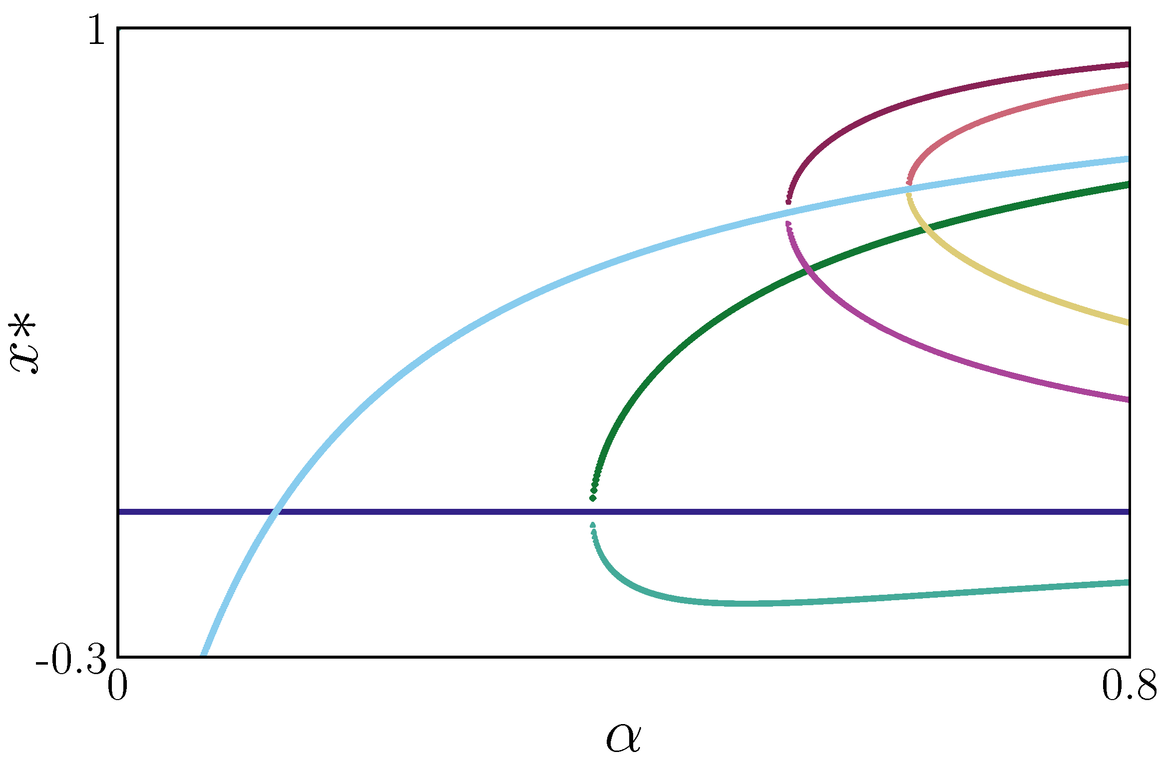
To explain the bifurcations displayed by bifurcation diagrams, we compute the stability of the fixed points for the maps $\overline{f}(x,y)$ and ${\overline{f}}^2(x,y)=\overline{f}\circ \overline{f}(x,y)$. In Figure 4, we observe the progression of the fixed points for ${\overline{f}}^2(x,y)$ as the control parameter $\alpha$ is modified.

The two eigenvalues of the Jacobian matrix for the fixed point ($x_2*,y_2*$), given by the yellow curve in Figure 1 and light blue one in Figure 4, exit the unit circle for different values of $\alpha$: one for $\alpha =0.53$ and another for $\alpha =0.62$. The first eigenvalue has a strong influence on generating the red bifurcation diagram of Figure 3. However, the blue bifurcation diagram starts in the instability produced by the second eigenvalue. Also, in Figure 4, we can observe the instability and generation of new fixed points shown by red and blue curves.

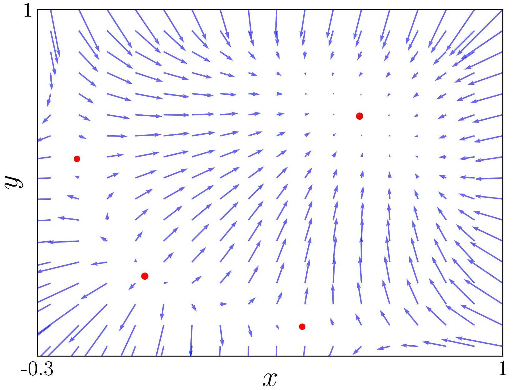
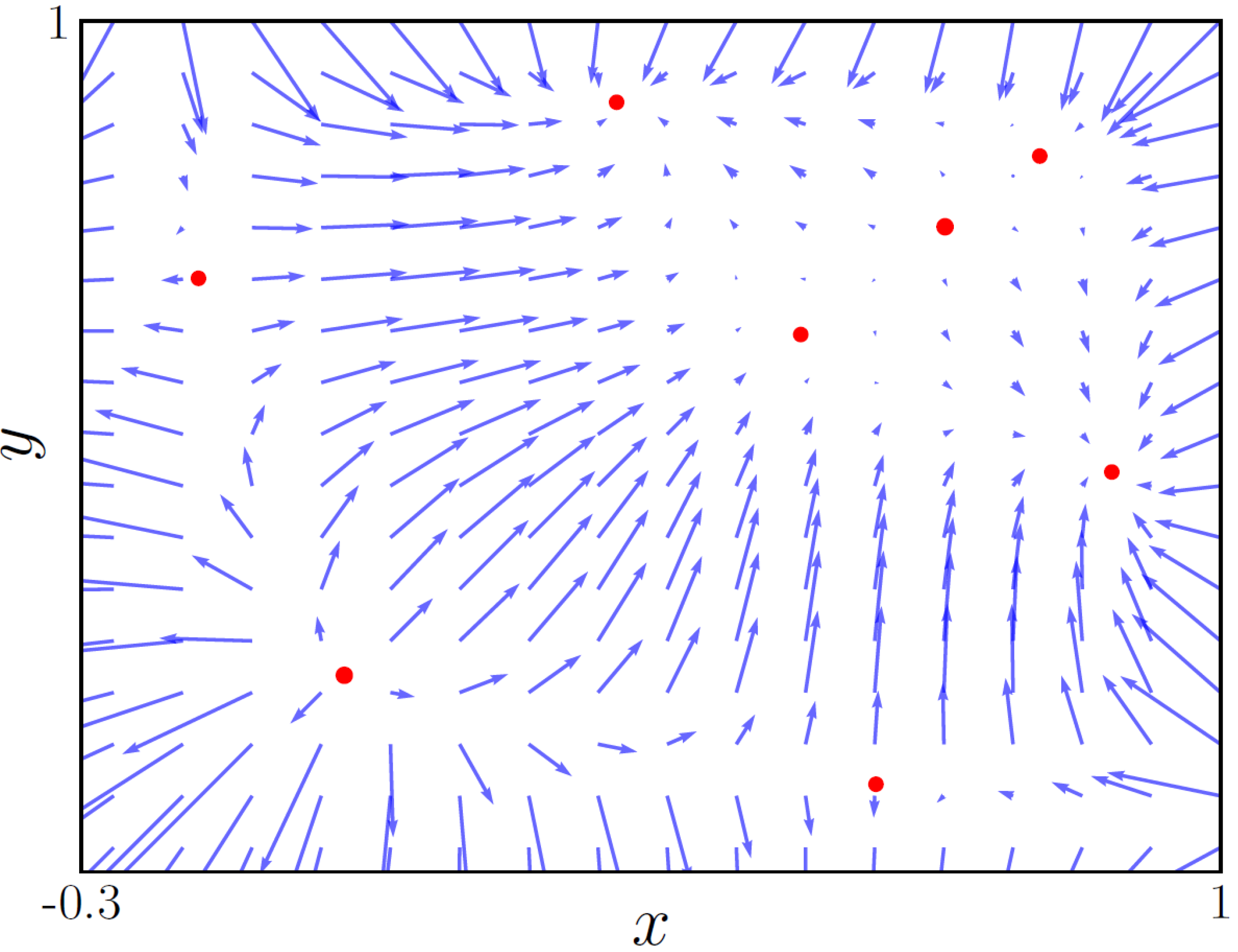
On the other hand, Figure 5, Figure 6, Figure 7 and Figure 8 displays the vector field in the $\left(x,y\right)$ plane together with the fixed points of map ${\overline{f}}^2(x,y)$ that appear as $\alpha$ grows.

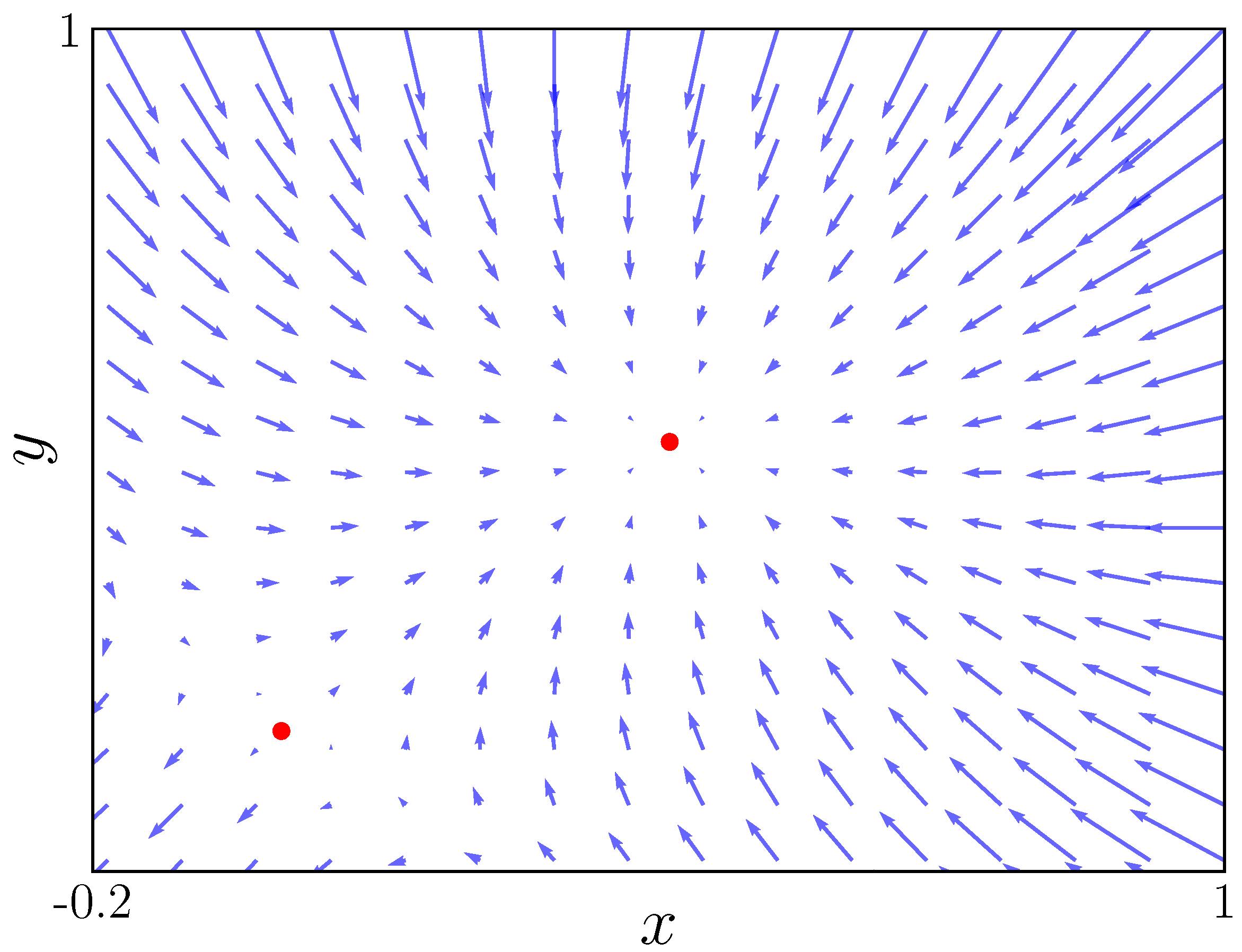
Figure 5 shows the vector field for $\alpha =0.3$. In this figure, we can see that there are only two fixed points which are shown in Figure 1 as blue and yellow lines. One fixed point is at $\left(0,0\right)$, and it is unstable, with the other one being stable at approximately $\left(0.42,0.42\right)$. As we move to Figure 6, with an $\alpha$ value $0.5$, we observe the bifurcation occurring at point $\left(0,0\right)$ and two more fixed points appearing. These two fixed points are saddle points, they attract alongside a direction and repel alongside the other. Figure 7 shows two new fixed points corresponding to the bifurcation shown in the violet solution of Figure 4. Finally, in Figure 8 ($\alpha =0.65$), the directional field shows the appearance of a pair of fixed points that correspond to the ones shown in pink and yellow in Figure 4, which are saddle points with one eigenvalue inside the unit circle and the other outside of it.

Figure 9 shows the bifurcation diagram used in [29]. From the figure, we see that for values of $\alpha \sim 0.7$ and $\sim 0.8$, the map presents a more complex behavior than those observed in the directional field (see Figure 5, Figure 6, Figure 7 and Figure 8). There is a set of fixed points that meet the condition $x*=y*$, these fixed points correspond to the blue diagram shown in Figure 3, because solutions with $x=y$ decouple the system and transform it into two independent logistic maps (see blue diagram in Figure 3).

Figure 9 is only feasible if the initial conditions of the iterative process for each $\alpha$ are deliberately selected. For an $\alpha$ lower to $\sim 0.715$, the initial conditions must verify $x_0\ne y_0$. On the other hand, for an $\alpha$ greater than $\sim 0.715$, the initial conditions have to satisfy $x_0=y_0$.

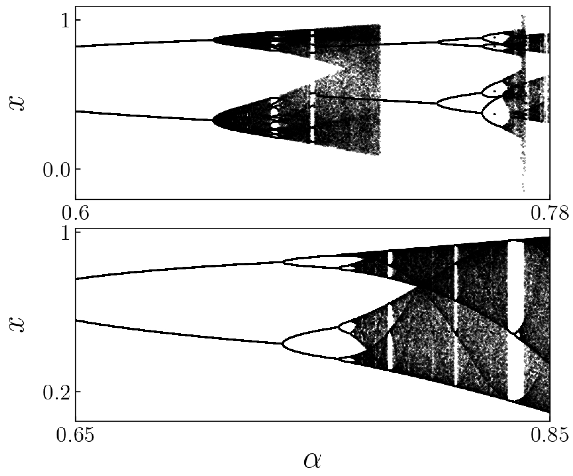
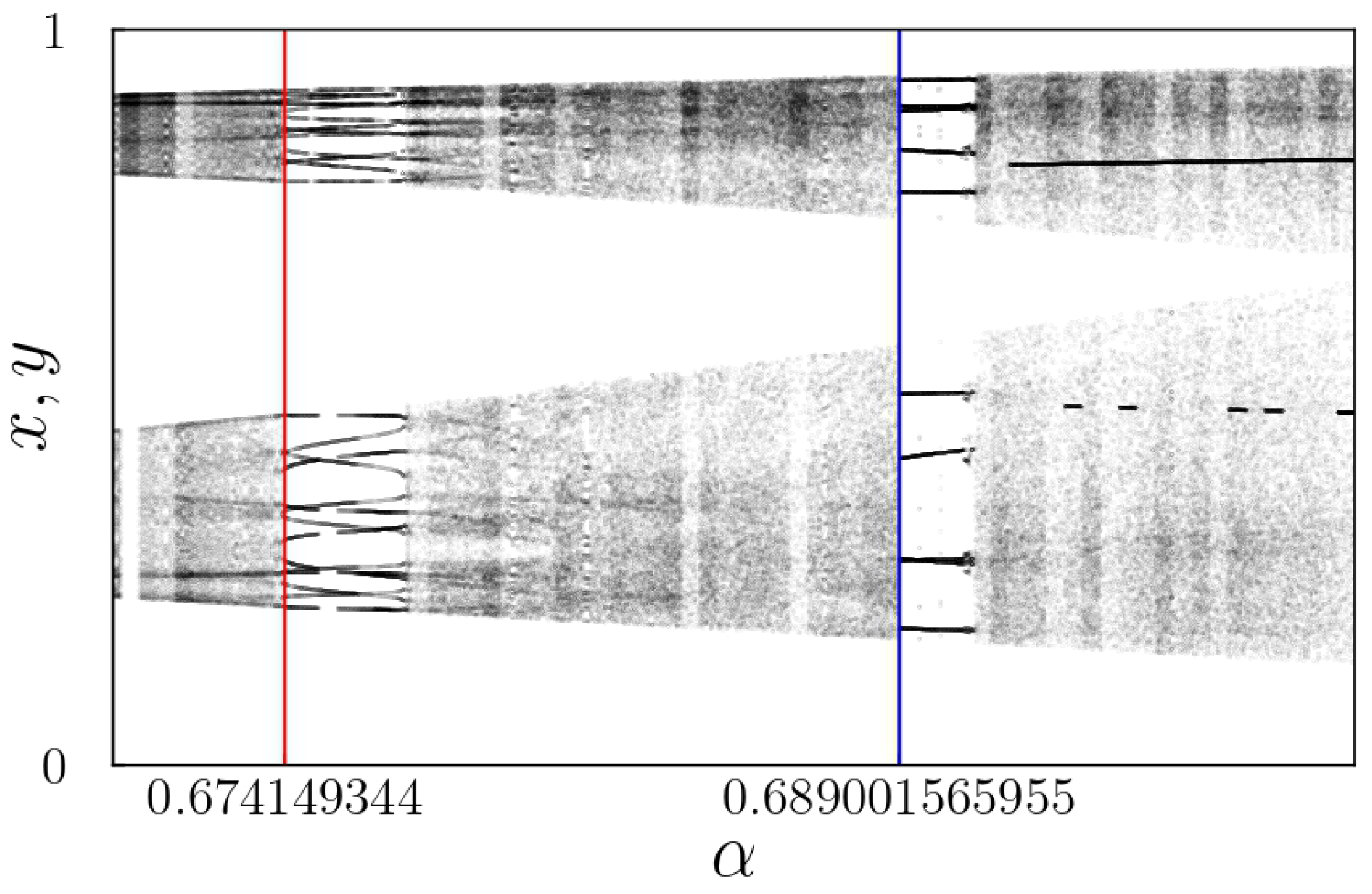
Figure 10 shows the bifurcation diagrams for x obtained for different initial conditions in the iterative process. The upper figure displays the diagram built with initial conditions $x_0\ne y_0$ for every $\alpha$, while the lower one was obtained only using $x_0=y_0$ as initial condition for every $\alpha$.

Figure 11 displays the relations between the variables x and y for the bifurcation diagrams of Figure 10. The left figure was calculated with initial conditions $x_0\ne y_0$ for $0.6\le \alpha <0.78$. The right figure was obtained using $x_0=y_0$ as initial condition for $0.65\le \alpha \le 0.85$.

For $\alpha$ greater than approximately $0.776$, the basin of attraction for the attractor depicted in the upper Figure 10 becomes nearly non-existent. Additionally, once $\alpha$ exceeds approximately $0.77$, the logistic attractor can be deemed a stable solution. This is achieved when the iterative processes are initiated on the bisector line in the $(x,y)$ plane, specifically on points where $(x_0=y_0)$.

3. Type I Intermittency

In this section, we examine three cases where type I intermittency occurs. We adhere to the criteria established by [29] to define type I intermittency for a two-dimensional map.

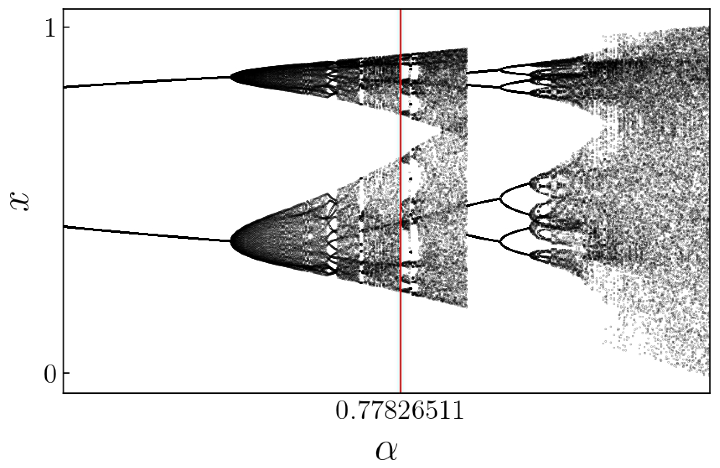
Figure 12 and Figure 13 present the regions of interest in the bifurcation diagrams, showing the period-14 solution at $\alpha \sim 0.674$ and a period-10 solution at $\alpha \sim 0.689$, both with $\beta =0.5$. With $\beta =0.3$, a chaotic solution is shown for $\alpha \sim 0.778$ near a period-14 solution.

The bifurcation diagram presented in Figure 12 shows a period-14 solution that occurs at approximately $\alpha \sim 0.674$ with $\beta =0.5$. The period-14 solution is placed between chaotic solutions for both lower and higher values of $\alpha$, indicating the potential presence of intermittency. Therefore, examining the $n+14$ map is particularly interesting in this context.

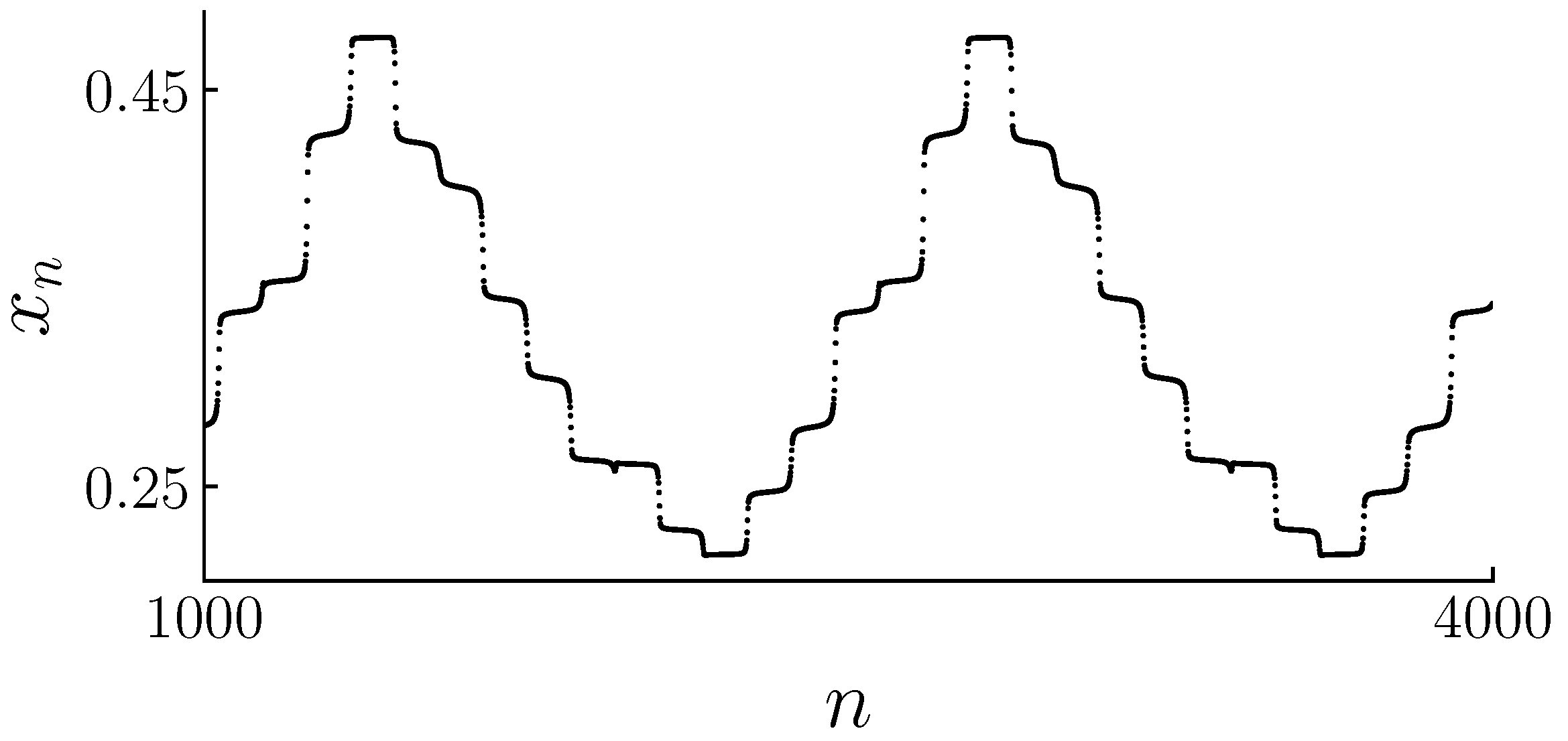
The solution for the map ${\overline{f}}^{14}(x,y)$, characterized by the parameter $\alpha =0.67414$, is shown in Figure 14. As we analyze the dynamics of the system, we can observe that the trajectory initially follows one branch of the attractor for a certain duration. Subsequently, it transitions to the alternate branch, and this pattern continues in a cyclic fashion, occurring a total of fourteen times. This repetitive switching between branches culminates in the formation of a limit cycle solution.

When we examine the trajectory in the two-dimensional state space $(x,y)$, it delineates a closed curve, as shown in Figure 15. This closed curve is indicative of the periodic nature of the oscillations within the system, demonstrating how the state variables evolve over time in a limit cycle.

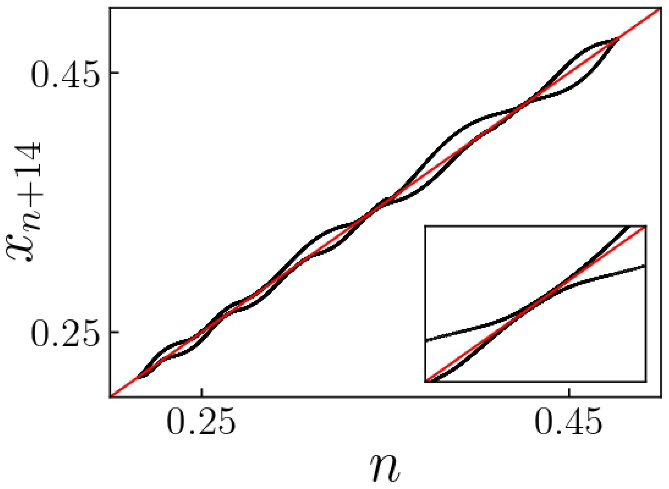
To gain a better understanding of the behavior of the solution, it is useful to analyze the map of $x_{n+14}$ versus $x_n$ for ${\overline{f}}^{14}(x,y)$. In Figure 16, we observe that the plateaus shown in Figure 14 are the result of the system solution approaching the bisector line $x_n=x_{n+14}$. This proximity of the map to the bisector line causes the trajectory to stay close for several iterations before being rapidly expelled and transported to a new region near the bisector line. Each time the trajectory approaches the line $x_n=x_{n+1}$, a narrow channel forms, resembling the behavior seen in type I intermittency in one-dimensional maps. In [29], this behavior is classified as type I intermittency, and a law for the mean or average laminar length is derived and compared with the results found for one-dimensional systems using the classic theory of chaotic intermittency.

The laminar length, in the context of intermittency, refers to the duration of the laminar phase. This duration is measured in iterations for discrete-time systems. For one-dimensional maps experiencing type I intermittency, the laminar length is a function of the distance between the map and the bisector line, known as the channel. The average laminar length depends on the control parameter $\epsilon$ in the following way [27]:

$$〈l〉\sim {\displaystyle \frac{1}{\sqrt{\epsilon }}}$$

(8)

where $〈l〉$ is the average laminar length. In these systems, the value of $\epsilon$ is directly related to the distance between the map and the bisector line. This distance determines the width of the channel, which causes the trajectory to pass more slowly. In this region, the laminar flow characteristics of the intermittency phenomenon are defined.

The map ${\overline{f}}^{14}(x,y)$ showed a separation concerning the bisector line when the control parameter, defined as $\epsilon ={\alpha }_c-\alpha$, was modified. The critical value of $\alpha$ at which intermittency is said to start and the limit cycle is found is known as ${\alpha }_c$.

The laminar or regular interval is defined as the stages of evolution in which the trajectory did not significantly change position. These stages are understood as the plateaus in Figure 14. However, unlike in one-dimensional maps, the laminar region in two-dimensional maps is not connected. It consists of very confined domains through which the system rapidly jumps, generating a structure of multiple channels.

Figure 17 shows the influence of the control parameter $\epsilon$ on the distance between the map ${\overline{f}}^{14}(x,y)$ and the bisector. Note that as $\epsilon$ grows, the distance between ${\overline{f}}^{14}(x,y)$ and the bisector also increases.

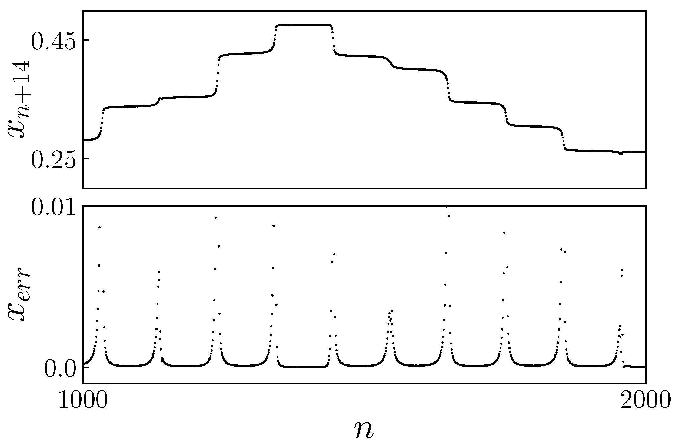
To measure how many iterations the trajectory needs to pass through each channel, we define the relative error function of the variable x as follows:

$$x_{err}=\left|{\displaystyle \frac{x_{n+14}-x_n}{x_n}}\right|$$

(9)

When the changes in the variable are small, $x_{err}\ll 1$, it is detected that the trajectory is in a laminar region-iterating within one of the fourteen channels. Laminar intervals are defined by a relative error that is less than a certain fixed threshold. Figure 18 shows the temporal evolution of the solution $x_{n+14}$ and the relative error function given by Equation (9).

The total number of iterations needed to complete the limit cycle was calculated by excluding the transition iterations between laminar regions, as they are insignificant when compared with others. The results obtained are presented in Figure 19. It shows the same slope as that achieved in [29].

To verify the previous results, we study two other cases. The first one uses $\alpha \approx 0.689$ and $\beta =0.5$. A period-10 solution in Figure 12 lies near a chaotic region which may indicate intermittency behavior as well as the period-14 solution in the same figure.

Figure 20 shows the change in laminar phase duration as the control parameter $\epsilon =\alpha -{\alpha }_c$ is modified. As $\epsilon$ grows ($\alpha$ moves away ${\alpha }_c$) the average laminar length decreases.

To determine the laminar or regular region, we use a second method. We define the distance between the map and the DHS surface. To determine this distance, we must find the minimum distance d from a 4th dimensional point $p_n=\left(x_n,y_n,x_{n+10},y_{n+10}\right)$ to a hyper-surface determined by DHS: $\{x_n,y_n,x_{n+10},y_{n+10}\in {\mathbf{R}}^4|x_n=x_{n+10}\wedge y_n=y_{n+10}\}$. So, we must find a point of the hyper-surface $p_s=\left(x_s,y_s,x_s,y_s\right)$ (because it satisfies the hyper-surface constraint) whose distance is the minimum to our point $p_n$. The 4th-dimensional Euclidean distance between the points will be

$$d=\sqrt{{\left(x_n-x_s\right)}^2+{\left(y_n-y_s\right)}^2+{\left(x_{n+10}-x_s\right)}^2+{\left(y_{n+10}-y_s\right)}^2},$$

(10)

minimizing the expression taking its derivatives with respect to $x_s$ and $y_s$ and equating them to zero, we obtain that

$$\begin{array}{cccc}\hfill & x_s={\displaystyle \frac{x_n+x_{n+10}}{2}}\hfill & \hfill & y_s={\displaystyle \frac{y_n+y_{n+10}}{2}}\hfill \end{array}$$

(11)

Figure 21 shows the temporal evolution of the variables $x_{n+10}$ and $y_{n+10}$, along with the distance to the DHS surface calculated using Equation (10).

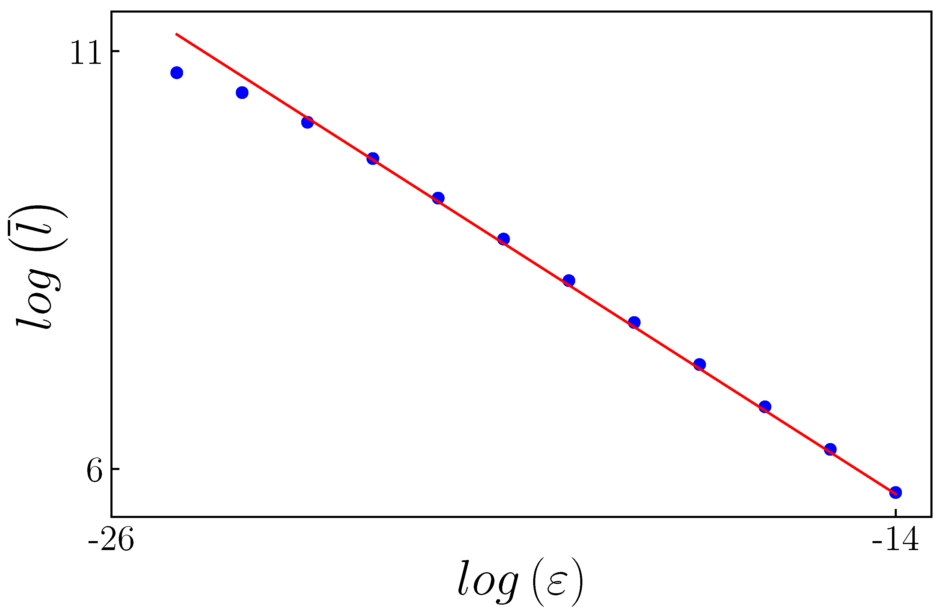
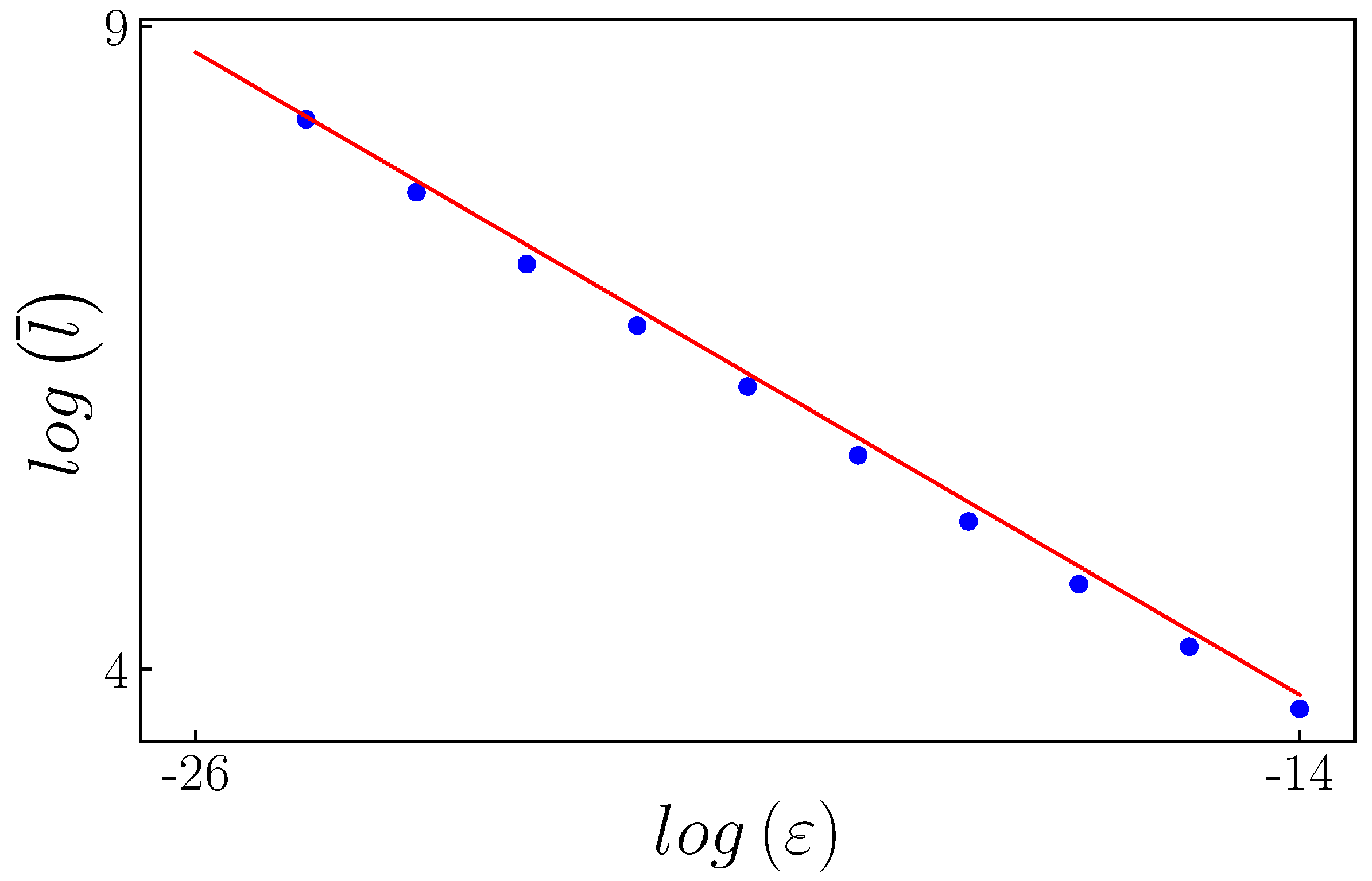
The numerical results for the characteristic relations are presented in Figure 22. This figure illustrates the relationship between the average or mean laminar length and the control parameter. The blue points represent the numerical results, while the red line is derived from Equation (8). It is noteworthy that there is good agreement between the numerical findings and the theoretical predictions.

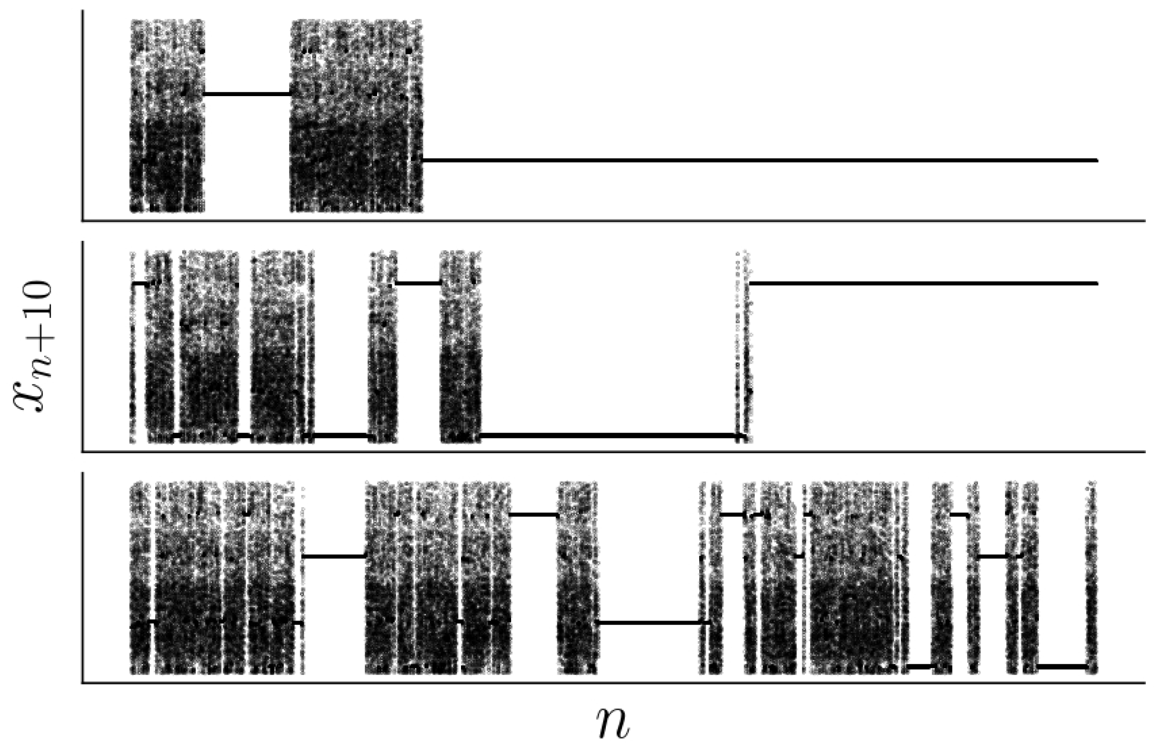
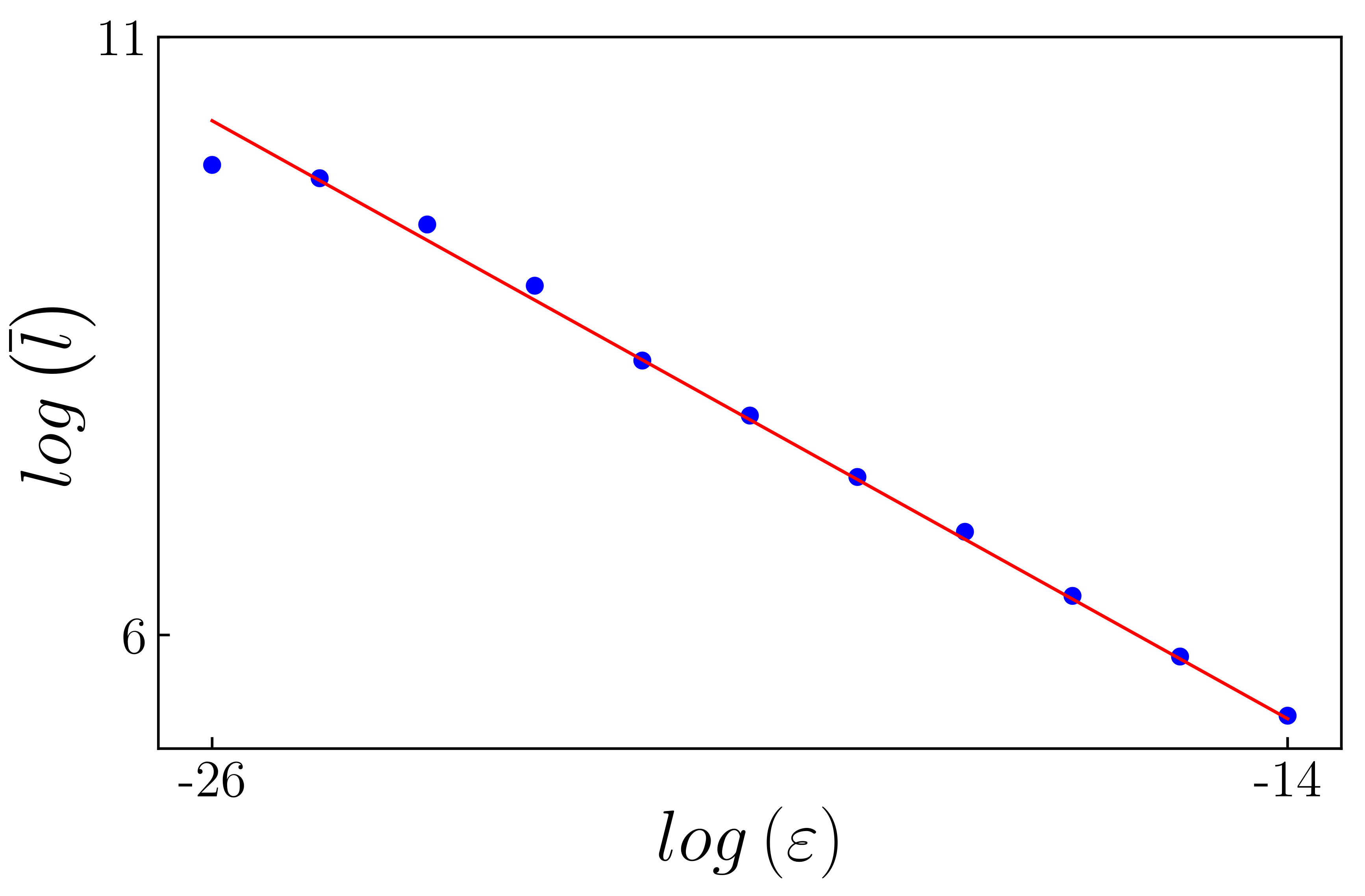
Finally, we analyze the following case: $\beta =0.3$ and $\alpha \approx 0.778$ (see Figure 13). To determine the laminar interval, we employed the distance between the map and the DHS surface given by Equation (8). The results for the average laminar length are shown in Figure 23.

For the three analyzed cases, we numerically confirm the validity of Equation (8) for the two-dimensional map studied in this investigation. This equation indicates that the same scaling behavior of the laminar length as a function of the control parameter observed in one-dimensional maps is also applicable for the map given by Equation (2).

4. Conclusions

We explore the intricate dynamics of the two-dimensional map defined by Equation (2). Our analysis includes calculating the solutions and their stability, bifurcation diagrams, and the basins of attraction for the system’s attractors. We observe that, for constant $\beta$, the solutions rapidly multiply when the control parameter $\alpha$ is altered, leading to significant changes in their stability. Additionally, we examine the intermittency phenomenon generated at distinct values of the control parameters $\alpha$ and $\beta$ and numerically derive the characteristic relationship associated with two-dimensional intermittency.

The system’s symmetry results in bifurcation diagrams that vary with the initial conditions. We discover that the symmetry of these initial conditions influences the solutions; different attractors emerge for cases where $x_0=y_0$ compared with $x_0\ne y_0$. Furthermore, we confirm that the bifurcations of fixed points and their stability changes depend on the chosen initial conditions.

We also investigate the relationship between the average laminar length and the control parameter $\epsilon ={\alpha }_c-\alpha$. To identify the laminar or regular phases in high-dimensional maps, we propose two alternative approaches (see Equations (9) and (10)). One method utilizes the error function, while the other calculates the distance between the map and the DHS surface. The first method is simpler, but the second method takes both variables into account. Despite these differences, both approaches yield the same results. Our calculations confirm that, for all studied cases, the relationship we obtain for type I intermittency aligns with what has been established for one-dimensional maps using classical theory.