Article

Fixed Time Synchronization of Stochastic Takagi–Sugeno Fuzzy Recurrent Neural Networks with Distributed Delay under Feedback and Adaptive Controls

1
Department of Mathematics, Northeast Forestry University, Harbin 150040, China
2
Engineering Research Center of Agricultural Microbiology Technology, Ministry of Education, Harbin 150080, China
3
Heilongjiang Provincial Key Laboratory of Ecological Restoration and Resource Utilization for Cold Region, Harbin 150080, China
4
School of Mathematical Science, Heilongjiang University, Harbin 150080, China
*
Author to whom correspondence should be addressed.
Axioms 2024, 13(6), 391; https://doi.org/10.3390/axioms13060391
Submission received: 6 April 2024 / Revised: 31 May 2024 / Accepted: 3 June 2024 / Published: 11 June 2024
(This article belongs to the Special Issue Recent Advances in Applied Mathematics and Artificial Intelligence)

Abstract

:
In this paper, the stochastic Takagi–Sugeno fuzzy recurrent neural networks (STSFRNNS) with distributed delay is established based on the Takagi–Sugeno (TS) model and the fixed time synchronization problem is investigated. In order to synchronize the networks, we design two kinds of controllers: a feedback controller and an adaptive controller. Then, we obtain the synchronization criteria in a fixed time by combining the Lyapunov method and the related inequality theory of the stochastic differential equation and calculate the stabilization time for the STSFRNNS. In addition, to verify the authenticity of the theoretical results, we use MATLABR2023A to carry out numerical simulation.

1. Introduction

Neural network models can be used to analyze and process data. By analyzing the data, the predicted value can be obtained, which is helpful to understand and grasp the change law of the data. Therefore, neural network models are widely used in economic projection, signal processing, intelligent control systems, optimization calculation, robot engineering, speech recognition, and other fields [1,2,3,4,5,6]. At the same time, recurrent neural networks (RNNS) have greatly attracted scholars. Recurrent neural networks are used in many fields, such as natural language processing, power industry, and various time series forecasting [7,8,9,10,11]. Time delay is a common problem in the research. In recurrent neural networks, time delay mainly includes the internal delay of recurrent neural network, the computation delay of each component, and the transmission delay of signal in the process of receiving and transmitting [12]. It is important to note that while the propagation of a signal is sometimes instantaneous, it can also be distributed over time, so we consider two kinds of time delays, namely, discrete and distributed time delays [13,14].
The actual operation of the system is often affected by random noise and human interference. Studying the dynamic system with random noise can reveal the effect of random noise on system behavior more clearly. Therefore, after establishing the neural network model, noise is introduced into the traditional differential equation model, and the deterministic model is transformed into the differential equation model with random disturbance. In 1996, Liao and Mao introduced random noise into neural networks for the first time [15]. Many scholars devote themselves to analyzing the dynamic properties of various kinds of stochastic neural networks [16,17,18].
In recent years, the Takagi–Sugeno fuzzy model has been widely used [19]. The TS fuzzy model converts normal fuzzy rules and their reasoning into a mathematical expression form. The essence is to establish multiple simple linear relationships through fuzzy division of the global nonlinear system, and perform fuzzy reasoning and judgment on the output of multiple models, which can represent complex nonlinear relationships. It was proposed by two scholars, Takagi and Sugeno, in 1985. The main idea of the TS fuzzy model is to express nonlinear systems with many similar line segments, that is, to convert the nonlinear problem that is not easy to consider into a problem on many small line segments. The TS fuzzy model is built on a set of nonlinear systems and described by IF-THEN rules, each of which represents a subsystem. It has been shown that the TS fuzzy system can approximate the arbitrary accuracy compact set of arbitrary continuous function R n . This allows designers to analyze and design nonlinear systems using traditional linear systems. On this basis, this paper extends the TS fuzzy model to describe delayed recurrent neural networks, and a stochastic recurrent neural network model based on TS fuzzy is established, which is simply called STSFRNNS.
As we all know, synchronization is one of the most basic and important problems in the study of neural network dynamic models [20,21,22]. In practice, the neural network often can not be automatically implemented and usually needs a suitable controller to be designed. Hence, researchers have come up with various control methods and techniques to achieve synchronization, including feedback control [23], adaptive control [24], and so on. These control methods provide great help to solve the problem of system synchronization and promote the development and progress of technology. In addition, synchronization is of great importance in many fields such as biology, climatology, sociology, ecology, and so on [25,26,27]. Therefore, it is greatly meaningful to study the synchronization characteristics for exploring recurrent neural networks.
This paper makes the following three contributions relative to the existing literature:
  • In this paper, the TS model is extended to recurrent neural networks, and synchronization properties are studied on this basis.
  • For each theoretical result and the generalization of the model, numerical simulation is given to verify its validity.
  • Two different kinds of control are used to study the synchronization property of the model, and the two kinds of control are compared.
N o t a t i o n s . Let ( Ω , F , F , P ) be a complete probability space with a filtration F = { F t } t 0 satisfying usual conditions, Ω is the set of all possible fundamental random events for a randomized trial, F is an algebra of σ , and P is a probability measure on a measurable space ( Ω , F ) . N-dimensional Brownian motion ω ( t ) is defined on ( Ω , F , F , P ) . Write | · | for the trace norm of matrices or the Euclidean norm of vectors. Let R n stand for n-dimensional Euclidean space. Let sign ( · ) be a symbolic function and A T represent the transpose of the vector (matrix) A. The notations R + = ( 0 , + ) and N = { 1 , 2 , , n } are used. And C 1 , 2 ( R + , R n × R + ) represents for the family of all nonnegative functions V ( ϕ ) differentiable twice consecutively over R n with respect to ϕ .

1.1. Model Formulations

The distributed delay is first introduced into the recurrent neural network, and the following model is obtained
ϕ ˙ ( t ) = A ϕ ( t ) + D g ( ϕ ( t ) ) + H g ( ϕ ( t τ ) ) + K t τ t g ( ϕ ( s ) ) d s + I ,
where vector I = ( I 1 , I 2 , , I n ) R n is used to represent a constant external input, ϕ ( t ) = [ ϕ 1 ( t ) , ϕ 2 ( t ) , , ϕ n ( t ) ] T R n is the neuronal state vector, g ( ϕ ( t ) ) = [ g 1 ( ϕ 1 ( t ) ) , g 2 ( ϕ 2 ( t ) ) , … g n ( ϕ n ( t ) ) ] T   R n denotes a nonlinear activation function, and we specify that g ( 0 ) = 0 .  A represents the rate matrix at which the neuronal potential resets to its resting state. Diagonal matrix A = diag[ a 1 , a 2 , a n ] and a i > 0, i = 1, 2, … n. τ > 0 denotes the time delay. D, H, and K are the connection weight matrix between neurons. D R n × n , H and K R n × n are the discrete delay connection weight matrices and distributed delay connection weight matrices, respectively.
The TS fuzzy model transforms the nonlinear system into a simpler continuous fuzzy system. By describing the state space of the fuzzy rules of local dependencies, dynamic character of system can be obtained. Under the description of the IF-THEN rule, every local dynamic has a linear input–output relationship. Combining with the TS fuzzy model, we propose the TS fuzzy recurrent neural networks with distributed and discrete delay. The Stochastic Takagi–Sugeno fuzzy recurrent neural networks distributed delay is shown below.
Rule:
IF: α 1 ( t ) i s M p 1 , α 2 ( t ) i s M p 2 , α r ( t ) i s M p r ,
THEN:
d ϕ ( t ) = [ A p ϕ ( t ) + D p g ( ϕ ( t ) ) + H p g ( ϕ ( t τ ) ) + K p t τ t g ( ϕ ( s ) ) d s + I ] d t + K p t τ t g ( ϕ ( s ) ) d s + I i ] d t + σ p ( t , ϕ ( t ) , ϕ ( t τ ) , t τ t g ( ϕ ( s ) ) d s ) d ω ( t ) ,
where σ z ( t ) are known variables, z = ( 1 , 2 , , r ) . M p l ( p 1 , 2 , , n , l 1 , 2 , , r ) is the fuzzy set.
Through the above discussion of IF-THEN rules, the STSFRNNS model is shown below
d ϕ ( t ) = p = 1 n β p ( α ( t ) ) { [ A p ϕ ( t ) + D p g ( ϕ ( t ) ) + H p g ( ϕ ( t τ ) ) + K p t τ t g ( ϕ ( s ) ) d s + I ] d t + σ p ( t , ϕ ( t ) , ϕ ( t τ ) , t τ t g ( ϕ ( s ) ) d s ) d ω ( t ) } / p = 1 n β p ( α ( t ) ) ,
where β p = l = 1 r M p l . Denote that η p ( α ( t ) ) = β p / p = 1 n β p . Then, the final output expression of STSFRNNS is as follows
d ϕ ( t ) = p = 1 n η p ( α ( t ) ) { [ A p ϕ ( t ) + D p g ( ϕ ( t ) ) + H p g ( ϕ ( t τ ) ) + K p t τ t g ( ϕ ( s ) ) d s + I ] d t + σ p ( t , ϕ ( t ) , ϕ ( t τ ) , t τ t g ( ϕ ( s ) ) d s ) d ω ( t ) } .
For each neuron, it is not difficult to derive the following expression
d ϕ i ( t ) = η i ( α i ( t ) ) { [ a i ϕ i ( t ) + j = 1 n d i j g ( ϕ j ( t ) ) + j = 1 n h i j g ( ϕ j ( t τ ) ) + j = 1 n k i j t τ t g ( ϕ i ( s ) ) d s + I i ] d t + σ i ( t , ϕ i ( t ) , ϕ i ( t τ ) , t τ t g ( ϕ i ( s ) ) d s ) d ω ( t ) } .
Considering (3) as the drive system, we can obtain the response system
d λ i ( t ) = η i ( α i ( t ) ) { [ u i ( t ) a i λ i ( t ) + j = 1 n d i j g ( λ j ( t ) ) + j = 1 n h i j g ( λ j ( t τ ) ) + j = 1 n k i j t τ t g ( λ i ( s ) ) d s + I i ] d t + σ i ( t , λ i ( t ) , λ i ( t τ ) , t τ t g ( λ i ( s ) ) d s ) d ω ( t ) } ,
where i = 1 , 2 , , n represents the neuron. In order to ensure (3) and (4) can achieve synchronization, u i is set as a controller. Let υ i ( t ) = λ i ( t ) ϕ i ( t ) be the error. Then, according to (3) and (4), the error system is shown below
d υ i ( t ) = η i ( α i ( t ) ) { [ u i ( t ) a i υ i ( t ) + j = 1 n d i j G ( υ j ( t ) ) + j = 1 n h i j G ( υ j ( t τ ) ) + j = 1 n k i j t τ t G ( υ i ( s ) ) d s ] d t + σ i ( t , υ i ( t ) , υ i ( t τ ) , t τ t G ( υ i ( s ) ) d s ) d ω ( t ) } ,
where
G ( υ i ( · ) ) = g ( λ i ( · ) ) g ( ϕ i ( · ) ) ,
and
σ i ( t , υ i ( t ) , υ i ( t τ ) , t τ t G ( υ i ( s ) ) d s ) = σ i ( t , λ i ( t ) , λ i ( t τ ) , t τ t g ( λ i ( s ) ) d s ) σ i ( t , ϕ i ( t ) , ϕ i ( t τ ) , t τ t g ( ϕ i ( s ) ) d s ) .

1.2. Assumption and Lemma

Assumption 1.
There is a positive number L 1 , for all s 1 , s 2 R , such that the function g ( · ) satisfies the bounded and Lipschitz conditions
| g ( s 1 ) g ( s 2 ) | L 1 | s 1 s 2 | .
Assumption 2.
σ satisfies locally Lipschitz and linear growth conditions. Moreover, σ satisfies
t r [ σ i ( t , υ i ( t ) , υ i ( t τ ) , t τ t G ( υ i ( s ) ) ) T σ i ( t , υ i ( t ) , υ i ( t τ ) , t τ t G ( υ i ( s ) ) ) ]   | ζ i υ i ( t ) | 2 + | ρ i υ i ( t τ ) | 2 + | ξ i t τ t G ( υ i ( s ) ) | 2 .
Lemma 1
([28]). If r 1 , r 2 , …, r n 0 , 0 < ρ < 1 , μ > 1 , then
i = 1 n r i ρ i = 1 n r i ρ ,
i = 1 n r i ρ n 1 μ i = 1 n r i μ .
Lemma 2
([29]). Consider the following systems,
d ϕ ( t ) = g ( t , ϕ ( t ) ) d t + h ( t , ϕ ( t ) ) d ω ( t ) ,
where ϕ ( t ) R n indicates the system status, ω ( t ) is a Brownian operation. Let ϕ ( t 0 ) = 0 and the time when stability is first reached is expressed as
T ( ϕ 0 , ω ) = i n f T 0 | κ 0 = 0 , t T .
If there is a Lyapunov function V(t, ϕ(t)) C 1 , 2 ( R + , R n × R + ) , which is a positive definite function and radially unbounded such that
L V ( ϕ ) λ 1 V α ( ϕ ) λ 2 V β ( ϕ ) .
Then the zero solution is stable with probability in stochastic fixed time, and
T ϵ = E ( T ( x 0 , ω ) ) 1 λ 1 1 α 1 + 1 λ 2 1 1 β .

2. Fixed Time Synchronization Analysis

In this section, the Lyapunov method and inequality relations are combined to obtain a general criterion for fixed time synchronization of STSFRNNS.

2.1. Feedback Control

To make the system realize fixed time synchronization, we first used feedback control. The feedback controller is shown below
u i ( t ) = ψ i υ i ( t ) μ 1 | υ i ( t ) | q sign ( υ i ( t ) ) γ 1 | υ i ( t ) | p sign ( υ i ( t ) ) j = 1 n κ i j | υ j ( t τ ) | sign ( υ i ( t ) ) 1 2 j = 1 n ι i j t τ t | υ i ( t ) | 2 d s υ i ( t ) | υ i ( t ) | 2 , υ i ( t ) 0 , j = 1 n o i j | υ i ( t τ ) | 2 | υ i ( t ) | sign ( υ i ( t ) ) 0 , υ i ( t ) = 0 ,
where i N , the constant number ψ i is the gain coefficient, and κ i j , ι i j , o i j , μ 1 , γ 1 are definite constants. The real number p and q satisfies p > 1 and 0 < q < 1 , respectively. In all subsequent proofs, for ease of representation, denote
υ i T ( t ) υ i ( t ) = υ i ˜ ( t ) , and i = 1 n j = 1 n = i , j = 1 n .
Theorem 1.
Under Assumptions 1 and 2, if the following four inequalities are satisfied. Then, under feedback control (6), systems (3) and (4) are synchronized within a fixed time.
2 a i 2 ψ i + ζ i + j = 1 n ( L 1 d i j + L 1 d j i + k i j ) 0 , 2 j = 1 n L 1 h i j j = 1 n κ i j 0 , ξ i + j = 1 n τ k j i ( L 1 ) 2 j = 1 n ι i j 0 , ρ i j = 1 n o i j 0 .
In addition, the following equation is used to represent the stabilization time
T ϵ = 1 μ 1 1 1 q + 1 γ 1 n 1 p 1 p 1 .
Proof. 
To prove Theorem 1, we construct V ( t , υ i ( t ) ) = i = 1 n υ i ˜ ( t ) . Then
L V = 2 i = 1 n η i ( α i ( t ) ) υ i T ( t ) [ u i ( t ) a i υ i ( t ) + j = 1 n d i j G ( υ j ( t ) ) + j = 1 n h i j G ( υ j ( t τ ) ) + j = 1 n k i j t τ t G ( υ i ( s ) ) d s ] d t + i = 1 n t r [ σ i ( t , υ i ( t ) , υ i ( t τ ) , t τ t G ( υ i ( s ) ) ) T σ i ( t , υ i ( t ) , υ i ( t τ ) , t τ t G ( υ i ( s ) ) ) ]
Note that
2 i = 1 n υ i T j = 1 n d i j G ( υ j ( t ) ) 2 i = 1 n | υ i ( t ) | j = 1 n d i j L 1 | υ j ( t ) | = 2 i , j = 1 n d i j L 1 | υ i ( t ) | | υ j ( t ) | i , j = 1 n d i j L 1 | υ i ( t ) | 2 + d i j L 1 | υ j ( t ) | 2 = i , j = 1 n d i j L 1 | υ i ( t ) | 2 + i , j = 1 n d i j L 1 | υ j ( t ) | 2 = i , j = 1 n d i j L 1 + d i j L 1 | υ i ( t ) | 2 .
And in a similar way, we have
2 i = 1 n υ i T ( t ) j = 1 n h i j G ( υ i ( t τ ) ) 2 i , j = 1 n h i j L 1 | υ i ( t ) | | υ j ( t τ ) | .
Moreover, it is given by the Cauchy–Schwarz inequality that
i = 1 n υ i T ( t ) j = 1 n k i j t τ t G ( υ i ( s ) ) d s i , j = 1 n k i j | υ i ( t ) | t τ t G ( υ i ( s ) ) d s i , j = 1 n k i j | υ i ( t ) | 2 + t τ t G ( υ i ( s ) ) d s 2 i , j = 1 n k i j | υ i ( t ) | 2 + i , j = 1 n k i j τ t τ t ( G ( υ i ( s ) ) ) 2 d s i , j = 1 n k i j | υ i ( t ) | 2 + i , j = 1 n k i j ( L 1 ) 2 t τ t | υ i ( s ) | 2 d s ,
and
2 i = 1 n υ i ( t ) u i 2 i = 1 n ψ i | υ i ( t ) | 2 i , j = 1 n κ i j | υ i ( t ) | | υ j ( t τ ) | 2 μ 1 i = 1 n υ i ˜ ( t ) 1 + q 2 2 γ 1 n 1 p i = 1 n υ i ˜ ( t ) 1 + p 2 i , j = 1 n ι i j t τ t | υ j ( s ) | 2 d s j = 1 n o i j | υ i ( 1 τ ) | 2 .
Therefore,
L V i = 1 n η i ( α i ( t ) ) 2 a i 2 ψ i + j = 1 n ( d i j L 1 + d j i L 1 ) + j = 1 n ( k i j ) + ζ | υ i ( t ) | 2 + i = 1 n η i ( α i ( t ) ) 2 j = 1 n h i j L 1 2 j = 1 n κ i j | υ i ( t ) | | υ j ( t τ ) | + i = 1 n η i ( α i ( t ) ) ξ i + j = 1 n τ k i j ( L 1 ) 2 j = 1 n ι i j t τ t | υ i ( s ) | 2 d s + i = 1 n η i ( α i ( t ) ) ρ i j = 1 n o i j | υ i ( t τ ) | 2 2 μ 1 i = 1 n υ i ˜ ( t ) 1 + q 2 2 γ 1 n 1 p i = 1 n υ i ˜ ( t ) 1 + p 2
Combined with the inequality relation in Theorem 1, it can finally be obtained
L V 2 μ 1 i = 1 n υ i ˜ ( t ) 1 + q 2 2 γ 1 n 1 p i = 1 n υ i ˜ ( t ) 1 + p 2 2 μ 1 ( V ( t , υ i ( t ) ) ) 1 + q 2 2 γ 1 n 1 p ( V ( t , υ i ( t ) ) ) 1 + p 2 .
By Lemma 2, the stability time can be calculated
T ϵ = 1 μ 1 1 1 q + 1 γ 1 n 1 p 1 p 1 .

2.2. Adaptive Control

In feedback control, the coefficient ψ i is not easy to determine. In order to achieve better synchronization control, we set up adaptive control here
u i ( t ) = ψ i ( t ) υ i ( t ) μ 2 | υ i ( t ) | q sign ( υ i ( t ) ) γ 2 | υ i ( t ) | p sign ( υ i ( t ) ) j = 1 n κ i j | υ j ( t τ ) | sign ( υ i ( t ) ) 1 2 j = 1 n ι i j t τ t | υ i ( t ) | 2 d s υ i ( t ) | υ i ( t ) | 2 , υ i ( t ) 0 , j = 1 n o i j | υ i ( t τ ) | 2 | υ i ( t ) | sign ( υ i ( t ) ) 0 , υ i ( t ) = 0 .
The adaptive control gain is represented by ψ i ( t ) and the designed adaptive rate is
ψ ˙ i ( t ) = υ i ˜ ( t ) μ 2 sign ( ψ i ( t ) ψ 1 ) ( ψ i ( t ) ψ 1 ) q γ 2 sign ( ψ i ( t ) ψ 1 ) ( ψ i ( t ) ψ 1 ) p ,
where ψ 1 is the undetermined constant. Then the synchronization criterion of STSFRNNS under adaptive control (7) can be obtained.
Theorem 2.
Under Assumptions 1 and 2, if the following four inequalities are satisfied, then systems (3) and (4) are synchronized in probability in a fixed time under adaptive controller (7).
2 a i 2 ψ 1 + ζ i + j = 1 n ( L 1 d i j + L 1 d j i + k i j ) 0 , 2 j = 1 n L 1 h i j j = 1 n κ i j 0 , ξ i + j = 1 n τ k j i ( L 1 ) 2 j = 1 n ι i j 0 , ρ i j = 1 n o i j 0 .
In addition, the following equation is used to represent the stabilization time
T ϵ = 1 μ 2 1 1 q + 1 γ 2 n 1 p 1 p 1 .
Proof. 
To prove Theorem 2, we construct V ( t , υ i ( t ) ) = i = 1 n υ i ˜ ( t ) + i = 1 n ( ψ i ( t ) ψ 1 ) 2 . Then
L V = 2 i = 1 n η i ( α i ( t ) ) υ i T [ a i υ i ( t ) + j = 1 n d i j G ( υ j ( t ) ) + j = 1 n h i j G ( υ j ( t τ ) ) + j = 1 n k i j t τ t G ( υ i ( s ) ) d s + u i ( t ) ] d t + i = 1 n t r [ σ i ( t , υ i ( t ) , υ i ( t τ ) , t τ t G ( υ i ( s ) ) ) T σ i ( t , υ i ( t ) , υ i ( t τ ) , t τ t G ( υ i ( s ) ) ) ] + 2 i = 1 n ( ψ i ( t ) ψ 1 ) · ψ ˙ i ( t ) .
Note that
2 i = 1 n υ i T u i ( t ) + 2 i = 1 n ( ψ i ( t ) ψ 1 ) · ψ ˙ i ( t ) = 2 i = 1 n υ i T ( ψ i ( t ) υ i ( t ) μ 2 | υ i ( t ) | q sign ( υ i ( t ) ) γ 2 | υ i ( t ) | p sign ( υ i ( t ) ) j = 1 n o i j | υ i ( t τ ) | 2 | υ i ( t ) | sign ( υ i ( t ) ) j = 1 n κ i j | υ j ( t τ ) | sign ( υ i ( t ) ) 1 2 j = 1 n ι i j t τ t | υ i ( t ) | 2 d s υ i ( t ) | υ i ( t ) | 2 ) + 2 i = 1 n ( ψ i ( t ) ψ 1 ) ( υ i T ( t ) υ i ( t ) μ 2 sign ( ψ i ( t ) ψ 1 ) ( ψ i ( t ) ψ 1 ) q γ 2 sign ( ψ i ( t ) ψ 1 ) ( ψ i ( t ) ψ 1 ) p ) = 2 i = 1 n υ i T ( ( ψ i ( t ) ψ 1 ) υ i ( t ) μ 2 | υ i ( t ) | q sign ( υ i ( t ) ) γ 2 | υ i ( t ) | p sign ( υ i ( t ) ) j = 1 n o i j | υ i ( t τ ) | 2 | υ i ( t ) | sign ( υ i ( t ) ) j = 1 n κ i j | υ j ( t τ ) | sign ( υ i ( t ) ) 1 2 j = 1 n ι i j t τ t | υ i ( t ) | 2 d s υ i ( t ) | υ i ( t ) | 2 ) + 2 i = 1 n ( ψ i ( t ) ψ 1 ) ( υ i ˜ ( t ) μ 2 sign ( ψ i ( t ) ψ 1 ) ( ψ i ( t ) ψ 1 ) q γ 2 sign ( ψ i ( t ) ψ 1 ) ( ψ i ( t ) ψ 1 ) p 2 i = 1 n ψ 1 υ i ˜ ( t ) ) 2 i , j = 1 n ρ i j | υ i ( t ) | | υ j ( t τ ) | i , j = 1 n ι i j t τ t | υ i ( t ) | 2 d s 2 i , j = 1 n o i j | υ i ( t τ ) | 2 2 μ 1 i = 1 n υ i ˜ ( t ) 1 + q 2 2 γ 1 n 1 p i = 1 n υ i ˜ ( t ) 1 + p 2 2 μ 2 i = 1 n ( ψ i ( t ) ψ 1 ) 1 + q 2 γ 2 n 1 p i = 1 n ( ψ i ( t ) ψ 1 ) 1 + p 2 i = 1 n ψ 1 υ i ˜ ( t ) .
It follows that
L V i = 1 n η i ( α i ( t ) ) 2 a i 2 ψ 1 + j = 1 n ( d i j L 1 + d j i L 1 ) + j = 1 n ( k i j ) + ζ | υ i ( t ) | 2 + i = 1 n η i ( α i ( t ) ) 2 j = 1 n h i j L 1 2 j = 1 n κ i j | υ i ( t ) | | υ j ( t τ ) | + i = 1 n η i ( α i ( t ) ) ξ i + j = 1 n τ k i j ( L 1 ) 2 j = 1 n ι i j t τ t | υ i ( s ) | 2 d s + i = 1 n η i ( α i ( t ) ) ρ i j = 1 n o i j | υ i ( t τ ) | 2 2 μ 2 i = 1 n υ i ˜ ( t ) 1 + q 2 2 γ 2 n 1 p i = 1 n υ i ˜ ( t ) 1 + p 2 2 μ 2 i = 1 n ( ψ i ( t ) ψ 1 ) 1 + q 2 γ 2 n 1 p i = 1 n ( ψ i ( t ) ψ 1 ) 1 + p .
Combined with the inequality relation in Theorem 2, it can finally be obtained
L V 2 μ 2 i = 1 n υ i ˜ ( t ) 1 + q 2 2 γ 2 n 1 p i = 1 n υ i ˜ ( t ) 1 + p 2 2 μ 2 i = 1 n ( ψ i ( t ) ψ 1 ) 1 + q 2 γ 2 n 1 p i = 1 n ( ψ i ( t ) ψ 1 ) 1 + p 2 μ 2 i = 1 n υ i ˜ ( t ) 1 + q 2 2 γ 2 n 1 p i = 1 n υ i ˜ ( t ) 1 + p 2 2 μ 2 i = 1 n ( ψ i ( t ) ψ 1 ) 2 1 + q 2 2 γ 2 n 1 p i = 1 n ( ψ i ( t ) ψ 1 ) 2 1 + p 2 2 μ 2 i = 1 n υ i ˜ ( t ) + i = 1 n ( ψ i ( t ) ψ 1 ) 2 1 + q 2 2 γ 2 n 1 p i = 1 n υ i ˜ ( t ) + i = 1 n ( ψ i ( t ) ψ 1 ) 2 1 + p 2 2 μ 2 V ( t , υ i ( t ) ) 1 + q 2 2 γ 2 n 1 p V ( t , υ i ( t ) ) 1 + p 2 .
By Lemma 2, the stability time can be calculated
T ϵ = 1 μ 1 1 1 q + 1 γ 1 n 1 p 1 p 1 .

3. Model Improvement and Extension

Modification of the Model Based on the Actual Situation

Usually, the past state of the recurrent neural network system will inevitably have an impact on the current state. That is, the evolution trend of the system depends not only on the system’s current state, but also on the state of a certain moment or several moments in the past. In this section, we introduce distributed and discrete time-varying delay in the model and consider the following system
d ϕ i ( t ) = η i ( α i ( t ) ) { [ a i ϕ i ( t ) + j = 1 n d i j g ( ϕ j ( t ) ) + j = 1 n h i j g ( ϕ j ( t w ( t ) ) ) + j = 1 n k i j t τ ( t ) t g ( ϕ i ( s ) ) d s + I i ] d t + σ i ( t , ϕ i ( t ) , ϕ i ( t w ( t ) ) , t τ ( t ) t g ( ϕ i ( s ) ) d s ) d ω ( t ) } ,
where w ( t ) and τ ( t ) are time-varying delays and satisfy 0 < w ( t ) < 1 , 0 < τ ( t ) < 1 . In this section, considering system (8) as the driving system, there is the following response system
d λ i ( t ) = η i ( α i ( t ) ) { [ u i ( t ) a i λ i ( t ) + j = 1 n d i j g ( λ j ( t ) ) + j = 1 n h i j g ( λ j ( t w ( t ) ) ) + j = 1 n k i j t τ ( t ) t g ( λ i ( s ) ) d s + I i ] d t + σ i ( t , λ i ( t ) , λ i ( t w ( t ) ) , t τ ( t ) t g ( λ i ( s ) ) d s ) d ω ( t ) } .
According to (8) and (9), the error system is
d υ i ( t ) = η i ( α i ( t ) ) { [ u i ( t ) a i υ i ( t ) + j = 1 n d i j G ( υ j ( t ) ) + j = 1 n h i j G ( υ j ( t w ( t ) ) ) + j = 1 n k i j t τ ( t ) t G ( υ i ( s ) ) d s ] d t + σ i ( t , υ i ( t ) , υ i ( t w ( t ) ) , t τ ( t ) t G ( υ i ( s ) ) d s ) d ω ( t ) } ,
with
σ i ( t , υ i ( t ) , υ i ( t w ( t ) ) , t τ ( t ) t G ( υ i ( s ) ) d s ) = σ i ( t , λ i ( t ) , λ i ( t w ( t ) ) , t τ ( t ) t g ( λ i ( s ) ) d s ) σ i ( t , ϕ i ( t ) , ϕ i ( t w ( t ) ) , t τ ( t ) t g ( ϕ i ( s ) ) d s ) .
Let σ satisfy the locally Lipschitz and linear growth conditions. Moreover, σ satisfies
t r [ σ i ( t , υ i ( t ) , υ i ( t w ( t ) ) , t τ ( t ) t G ( υ i ( s ) ) ) T σ i ( t , υ i ( t ) , υ i ( t w ( t ) ) , t τ ( t ) t G ( υ i ( s ) ) ) ] | ζ i υ i ( t ) | 2 + | ρ i υ i ( t w ( t ) ) | 2 + | ξ i t τ t G ( υ i ( s ) ) | 2 .
For better study the synchronization properties, we consider adaptive control here
u i ( t ) = ψ i ( t ) υ i ( t ) μ 2 | υ i ( t ) | q sign ( υ i ( t ) ) γ 2 | υ i ( t ) | p sign ( υ i ( t ) ) j = 1 n κ i j | υ j ( t w ( t ) ) | sign ( υ i ( t ) ) 1 2 j = 1 n ι i j t τ ( t ) t | υ i ( t ) | 2 d s υ i ( t ) | υ i ( t ) | 2 , υ i ( t ) 0 , j = 1 n o i j | υ i ( t w ( t ) ) | 2 | υ i ( t ) | sign ( υ i ( t ) ) 0 , υ i ( t ) = 0 .
The adaptive control gain is represented by ψ i ( t ) and the designed adaptive rate is
ψ ˙ i ( t ) = υ i ˜ ( t ) μ 2 sign ( ψ i ( t ) ψ 1 ) ( ψ i ( t ) ψ 1 ) q γ 2 sign ( ψ i ( t ) ψ 1 ) ( ψ i ( t ) ψ 1 ) p ,
where ψ 1 is the undetermined constant. Then the synchronization criterion of STSFRNNS under adaptive control (11) can be obtained.
Theorem 3.
Under Assumptions 1 and 2, if the following four inequalities are satisfied, then systems (8) and (9) are synchronized in probability in a stochastic fixed time under adaptive control (11).
2 a i 2 ψ 1 + ζ i + j = 1 n ( L 1 d i j + L 1 d j i + k i j ) 0 , 2 j = 1 n L 1 h i j j = 1 n κ i j 0 , ξ i + j = 1 n w ( t ) k j i ( L 1 ) 2 j = 1 n ι i j 0 , ρ i j = 1 n o i j 0 .
In addition, the following equation is used to represent the stabilization time
T ϵ = 1 μ 1 1 1 q + 1 γ 1 n 1 p 1 p 1 .
Proof. 
To prove Theorem 3, we construct V ( t , υ i ( t ) ) = i = 1 n υ i ˜ ( t ) + i = 1 n ( ψ i ( t ) ψ 1 ) 2 . Then
L V = 2 i = 1 n η i ( α i ( t ) ) υ i T [ u i ( t ) a i υ i ( t ) + j = 1 n d i j G ( υ j ( t ) ) + j = 1 n h i j G ( υ j ( t w ( t ) ) ) + j = 1 n k i j t τ ( t ) t G ( υ i ( s ) ) d s ] d t + i = 1 n t r [ σ i ( t , υ i ( t ) , υ i ( t w ( t ) ) , t τ ( t ) t G ( υ i ( s ) ) ) T σ i ( t , υ i ( t ) , υ i ( t w ( t ) ) , t τ ( t ) t G ( υ i ( s ) ) ) ] + 2 i = 1 n ( ψ i ( t ) ψ 1 ) · ψ ˙ i ( t ) .
Note that
2 i = 1 n υ i T u i ( t ) + 2 i = 1 n ( ψ i ( t ) ψ 1 ) · ψ ˙ i ( t ) = 2 i = 1 n υ i T ( ψ i ( t ) υ i ( t ) j = 1 n κ i j | υ j ( t w ( t ) ) | sign ( υ i ( t ) ) 1 2 j = 1 n ι i j t τ ( t ) t | υ i ( t ) | 2 d s υ i ( t ) | υ i ( t ) | 2 j = 1 n o i j | υ i ( t w ( t ) ) | 2 | υ i ( t ) | sign ( υ i ( t ) ) μ 2 | υ i ( t ) | q sign ( υ i ( t ) ) γ 2 | υ i ( t ) | p sign ( υ i ( t ) ) ) + 2 i = 1 n ( ψ i ( t ) ψ 1 ) ( υ i ˜ ( t ) μ 2 sign ( ψ i ( t ) ψ 1 ) ( ψ i ( t ) ψ 1 ) q γ 2 sign ( ψ i ( t ) ψ 1 ) ( ψ i ( t ) ψ 1 ) p ) = 2 i = 1 n υ i T ( ( ψ i ( t ) ψ 1 ) υ i ( t ) j = 1 n κ i j | υ j ( t w ( t ) ) | sign ( υ i ( t ) ) 1 2 j = 1 n ι i j t τ ( t ) t | υ i ( t ) | 2 d s υ i ( t ) | υ i ( t ) | 2 j = 1 n o i j | υ i ( t w ( t ) ) | 2 | υ i ( t ) | sign ( υ i ( t ) ) μ 2 | υ i ( t ) | q sign ( υ i ( t ) ) γ 2 | υ i ( t ) | p sign ( υ i ( t ) ) ) + 2 i = 1 n ( ψ i ( t ) ψ 1 ) ( υ i ˜ ( t ) μ 2 sign ( ψ i ( t ) ψ 1 ) ( ψ i ( t ) ψ 1 ) q γ 2 sign ( ψ i ( t ) ψ 1 ) ( ψ i ( t ) ψ 1 ) p 2 i = 1 n ψ 1 υ i ˜ ( t ) ) . 2 i , j = 1 n ρ i j | υ i ( t ) | | υ j ( t w ( t ) ) | i , j = 1 n ι i j t τ ( t ) t | υ i ( t ) | 2 d s 2 i , j = 1 n o i j | υ i ( t w ( t ) ) | 2 2 μ 1 i = 1 n υ i ˜ ( t ) 1 + q 2 2 γ 1 n 1 p i = 1 n υ i ˜ ( t ) 1 + p 2 2 μ 2 i = 1 n ( ψ i ( t ) ψ 1 ) 1 + q 2 γ 2 n 1 p i = 1 n ( ψ i ( t ) ψ 1 ) 1 + p 2 i = 1 n ψ 1 υ i ˜ ( t ) .
Hence,
L V i = 1 n η i ( α i ( t ) ) 2 a i 2 ψ 1 + j = 1 n ( d i j L 1 + d j i L 1 ) + j = 1 n ( k i j ) + ζ | υ i ( t ) | 2 + i = 1 n η i ( α i ( t ) ) 2 j = 1 n h i j L 1 2 j = 1 n ϕ i j | υ i ( t ) | | υ j ( t w ( t ) ) | + i = 1 n η i ( α i ( t ) ) ξ i + j = 1 n w ( t ) k i j ( L 1 ) 2 j = 1 n ι i j t τ ( t ) t | υ i ( s ) | 2 d s + i = 1 n η i ( α i ( t ) ) ρ i j = 1 n o i j | υ i ( t w ( t ) ) | 2 2 μ 2 i = 1 n υ i ˜ ( t ) 1 + q 2 2 γ 2 n 1 p i = 1 n υ i ˜ ( t ) 1 + p 2 2 μ 2 i = 1 n ( ψ i ( t ) ψ 1 ) 1 + q 2 γ 2 n 1 p i = 1 n ( ψ i ( t ) ψ 1 ) 1 + p .
Combined with the inequality relation in Theorem 3, it can finally be obtained
L V 2 μ 2 i = 1 n υ i ˜ ( t ) 1 + q 2 2 γ 2 n 1 p i = 1 n υ i ˜ ( t ) 1 + p 2 2 μ 2 i = 1 n ( ψ i ( t ) ψ 1 ) 1 + q 2 γ 2 n 1 p i = 1 n ( ψ i ( t ) ψ 1 ) 1 + p 2 μ 2 i = 1 n υ i ˜ ( t ) 1 + q 2 2 γ 2 n 1 p i = 1 n υ i ˜ ( t ) 1 + p 2 2 μ 2 i = 1 n ( ψ i ( t ) ψ 1 ) 2 1 + q 2 2 γ 2 n 1 p i = 1 n ( ψ i ( t ) ψ 1 ) 2 1 + p 2 2 μ 2 i = 1 n υ i ˜ ( t ) + i = 1 n ( ψ i ( t ) ψ 1 ) 2 1 + q 2 . 2 γ 2 n 1 p i = 1 n υ i ˜ ( t ) + i = 1 n ( ψ i ( t ) ψ 1 ) 2 1 + p 2 2 μ 2 V ( t , υ i ( t ) ) 1 + q 2 2 γ 2 n 1 p V ( t , υ i ( t ) ) 1 + p 2
By Lemma 2, the stability time can be calculated
T ϵ = 1 μ 1 1 1 q + 1 γ 1 n 1 p 1 p 1 .

4. Numerical Simulation

The theoretical results in Section 3 prove the synchronization property of the STSFRNNS model. In order to verify the theoretical results, the numerical simulations of the motion trajectory of the system under two kinds of control are carried out, and the simulation results show that the theoretical results are valid. Taking N = 1 , 2 , , 8 , the expression of drive system (3) is
d ϕ i ( t ) = η i ( α i ( t ) ) { [ a i ϕ i ( t ) + j = 1 8 d i j g ( ϕ j ( t ) ) + j = 1 8 h i j g ( ϕ j ( t τ ) ) + j = 1 8 k i j t τ t g ( ϕ i ( s ) ) d s + I i ] d t + σ i ( t , ϕ i ( t ) , ϕ i ( t τ ) , t τ t g ( ϕ i ( s ) ) d s ) d ω ( t ) } ,
where i , j N , η i = 0.125 , a i = 1.75 , τ = 1 , I i = 0 , L 1 = 1 , g ( · ) = t a n ( · ) , and
σ i ( t , ϕ i ( t ) , ϕ i ( t τ ) , t τ t g ( ϕ i ( s ) ) d s ) = b i ϕ i ( t ) + c i ϕ i ( t τ ) + m i t τ t g ( ϕ i ( s ) d s .
Furthermore, let b i = c i = m i , and m 1 = 3 , m 2 = 3.5 , m 3 = 4 , m 4 = 4.5 , m 5 = 3 ,   m 6 = 3.5 ,   m 7 = 4 , m 8 = 4.5 . The values of k i j , d i j and h i j are listed in Table 1, Table 2 and Table 3 respectively.
Then the expression of the response system (4) is
d λ i ( t ) = η i ( α i ( t ) ) { [ u i ( t ) a i λ i ( t ) + j = 1 8 d i j g ( λ j ( t ) ) + j = 1 8 h i j g ( λ j ( t τ ) ) + j = 1 8 k i j t τ t g ( λ i ( s ) ) d s + I i ] d t + σ i ( t , λ i ( t ) , λ i ( t τ ) , t τ t g ( λ i ( s ) ) d s ) d ω ( t ) } .
It is not hard to obtain
σ 1 ( t , λ 1 ( t ) , λ 1 ( t τ ) , t τ t g ( λ 1 ( s ) ) d s ) = 3 λ 1 ( t ) + 3 λ 1 ( t τ ) + 3 t τ t g ( λ 1 ( s ) d s .
In addition, according to (12) and (13), the error system (5) is
d υ i ( t ) = η i ( α i ( t ) ) { [ a i υ i ( t ) + j = 1 8 d i j g ( υ j ( t ) ) + j = 1 8 h i j g ( υ j ( t τ ) ) + j = 1 8 k i j t τ t g ( υ i ( s ) ) d s + I i ] d t + σ i ( t , υ i ( t ) , υ i ( t τ ) , t τ t g ( υ i ( s ) ) d s ) d ω ( t ) } .

4.1. Numerical Simulation 1

To verify Theorem 1, the following numerical simulations show that the fixed time synchronization of (12) and (13) under the action of feedback control can be achieved. The controller (6) is
u i ( t ) = ψ i υ i ( t ) j = 1 8 κ i j | υ j ( t τ ) | sign ( υ i ( t ) ) 1 2 j = 1 8 ι i j t τ t | υ i ( t ) | 2 d s υ i ( t ) | υ i ( t ) | 2 μ 1 | υ i ( t ) | q sign ( υ i ( t ) ) γ 1 | υ i ( t ) | p sign ( υ i ( t ) ) , υ i ( t ) 0 , j = 1 8 o i j | υ i ( t τ ) | 2 | υ i ( t ) | sign ( υ i ( t ) ) 0 , υ i ( t ) = 0 ,
where ψ i = 50 ( i N ) , μ 1 = 0.6 , γ 1 = 0.8 , q = 0.2 , p = 1.2 , ι 11 = ι 22 = ι 33 = ι 44 = ι 55 = ι 66 = ι 77 = ι 88 = 4 , κ 11 = κ 22 = κ 33 = κ 44 = κ 55 = κ 66 = κ 77 = κ 88 = 5 . Any parameters else that are not mentioned are zero. According to the values of the above parameters, the conditions in Theorem 1 can be verified. That is,
2 a i 2 ψ i + ζ i + j = 1 8 ( L 1 d i j + L 1 d j i + k i j ) 0 2 j = 1 8 L 1 h i j j = 1 8 κ i j 0 ξ i + j = 1 8 τ k j i ( L 1 ) 2 j = 1 8 ι i j 0 ρ i j = 1 8 o i j 0 .
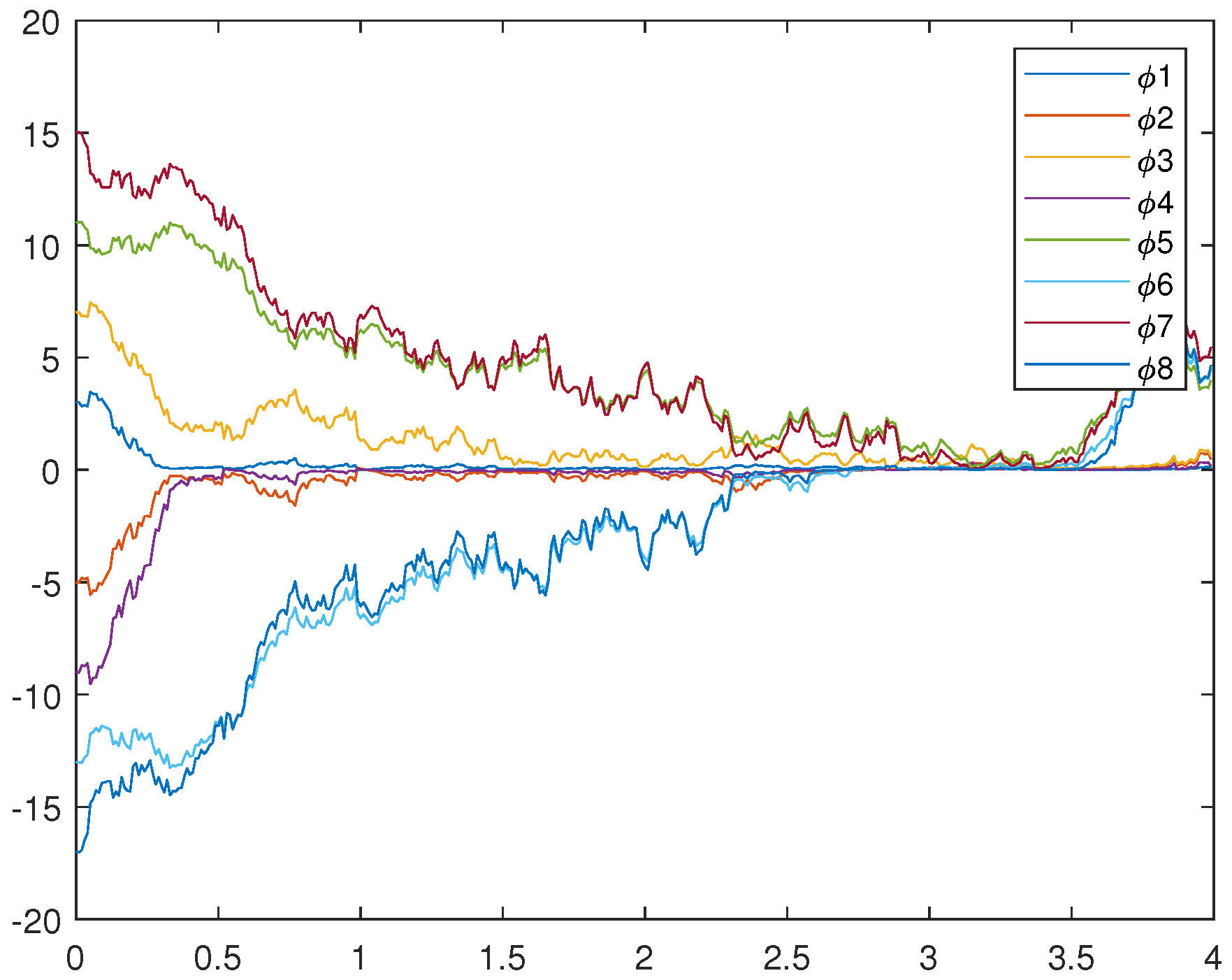
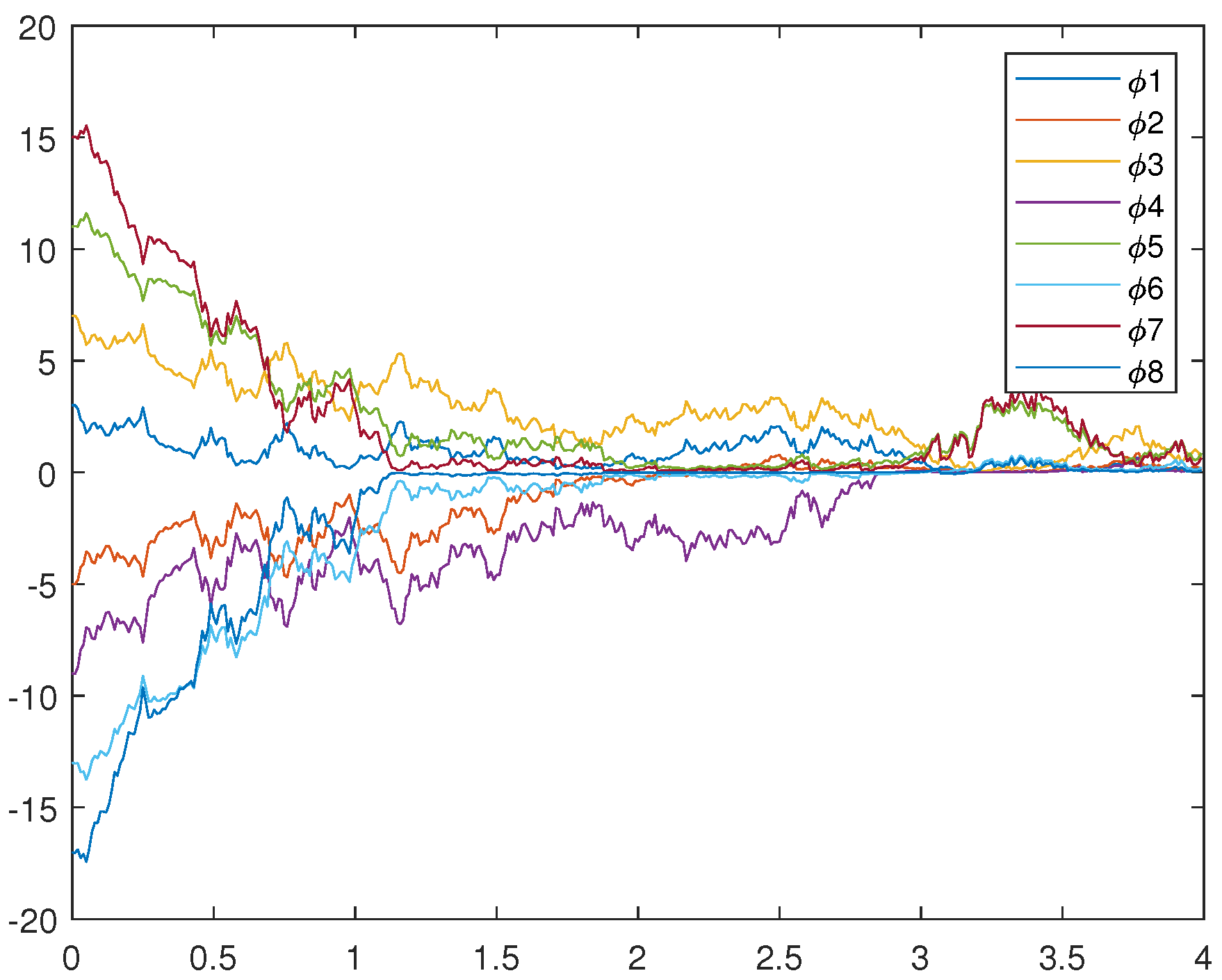
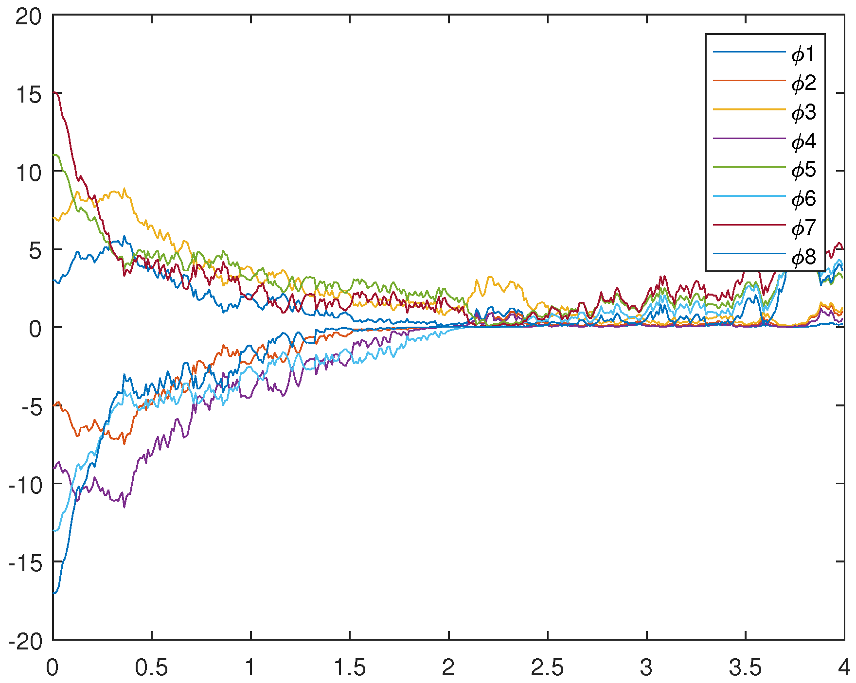
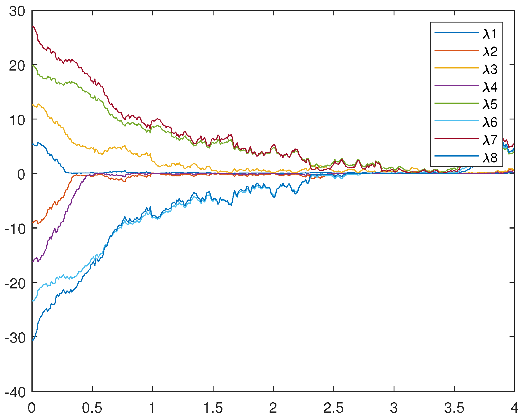
Figure 1 is an uncontrolled error system. It is not hard to find that the motion trajectory of the error system cannot achieve synchronization without adding the controller. Figure 2, Figure 3, and Figure 4 represent (12), (13), and (14), respectively. Figure 4 very intuitively shows that the trajectory of the error system tends to zero in a certain period of time, and the STSFRNNS model also gradually tends to synchronization.

4.2. Numerical Simulation 2

To verify Theorem 2, the following numerical simulations show that the fixed time synchronization of (12) and (13) under the action of adaptive control can be achieved.
u i ( t ) = ψ i ( t ) υ i ( t ) j = 1 8 κ i j | υ j ( t τ ) | sign ( υ i ( t ) ) 1 2 j = 1 8 ι i j t τ t | υ i ( t ) | 2 d s υ i ( t ) | υ i ( t ) | 2 μ 2 | υ i ( t ) | q sign ( υ i ( t ) ) γ 2 | υ i ( t ) | p sign ( υ i ( t ) ) , υ i ( t ) 0 , j = 1 8 o i j | υ i ( t τ ) | 2 | υ i ( t ) | sign ( υ i ( t ) ) 0 , υ i ( t ) = 0 ,
The adaptive control gain is represented by ψ i ( t ) and the designed adaptive rate is
ψ ˙ i ( t ) = υ i ˜ ( t ) μ 2 sign ( ψ i ( t ) ψ 1 ) ( ψ i ( t ) ψ 1 ) q γ 2 sign ( ψ i ( t ) ψ 1 ) ( ψ i ( t ) ψ 1 ) p ,
where ψ 1 = 85 , μ 2 = 0.6 , γ 2 = 0.8 , q = 0.2 , p = 1.2 , and the values not mentioned are the same as before. Any parameters else that are not mentioned are zero. According to the values of the above parameters, the conditions in Theorem 2 can be verified. That is,
2 a i 2 ψ 1 + ζ i + j = 1 8 ( L 1 d i j + L 1 d j i + k i j ) 0 , 2 j = 1 8 L 1 h i j j = 1 8 κ i j 0 , ξ i + j = 1 8 τ k j i ( L 1 ) 2 j = 1 8 ι i j 0 , ρ i j = 1 8 o i j 0 .
Figure 5, Figure 6, and Figure 7 represent the trajectory of (12), (13), and (14), respectively. Figure 7 very intuitively shows that the trajectory of the error system tends to zero in a certain period of time, and the STSFRNNS model also gradually tends to synchronization.

4.3. Brief Summary

From Figure 4 and Figure 7, it is not hard to find that the two controls designed above can make the STSFRNNS achieve fixed time synchronization. Compared with Figure 4, the convergence rate in Figure 7 is faster and the error system approaches 0 earlier. When other conditions remain unchanged, adaptive control is more suitable for STSFRNNS.

4.4. Numerical Simulation 3

To verify Theorem 3, the following numerical simulations shows that the fixed time synchronization of (12) and (13) under the action of adaptive control can be achieved.
u i ( t ) = ψ i ( t ) υ i ( t ) μ 2 | υ i ( t ) | q sign ( υ i ( t ) ) γ 2 | υ i ( t ) | p sign ( υ i ( t ) ) j = 1 8 κ i j | υ j ( t w ( t ) ) | sign ( υ i ( t ) ) 1 2 j = 1 8 ι i j t τ ( t ) t | υ i ( t ) | 2 d s υ i ( t ) | υ i ( t ) | 2 , υ i ( t ) 0 , j = 1 8 o i j | υ i ( t w ( t ) ) | 2 | υ i ( t ) | sign ( υ i ( t ) ) 0 , υ i ( t ) = 0 .
The adaptive control gain is represented by ψ i ( t ) and the designed adaptive rate is
ψ ˙ i ( t ) = υ i ˜ ( t ) μ 2 sign ( ψ i ( t ) ψ 1 ) ( ψ i ( t ) ψ 1 ) q γ 2 sign ( ψ i ( t ) ψ 1 ) ( ψ i ( t ) ψ 1 ) p .
According to the values of the above parameters, the conditions in Theorem 3 can be verified.
2 a i 2 ψ 1 + ζ i + j = 1 8 ( L 1 d i j + L 1 d j i + k i j ) 0 , 2 j = 1 8 L 1 h i j j = 1 8 κ i j 0 , ξ i + j = 1 8 τ ( t ) k j i ( L 1 ) 2 j = 1 8 ι i j 0 , ρ i j = 1 8 o i j 0 .
The drive system and response system are
d ϕ i ( t ) = η i ( α i ( t ) ) { [ a i ϕ i ( t ) + j = 1 8 d i j g ϕ j ( t ) ) + j = 1 8 h i j g ( ϕ j ( t w ( t ) ) ) + j = 1 8 k i j t τ ( t ) t g ( ϕ i ( s ) ) d s + I i ] d t + σ i ( t , ϕ i ( t ) , ϕ i ( t w ( t ) ) , t τ ( t ) t g ( ϕ i ( s ) ) d s ) d ω ( t ) } ,
and
d λ i ( t ) = η i ( α i ( t ) ) { [ u i ( t ) a i λ i ( t ) + j = 1 8 d i j g ( λ j ( t ) ) + j = 1 8 h i j g ( λ j ( t w ( t ) ) ) + j = 1 8 k i j t τ ( t ) t g ( λ i ( s ) ) d s + I i ] d t + σ i ( t , λ i ( t ) , λ i ( t w ( t ) ) , t τ ( t ) t g ( λ i ( s ) ) d s ) d ω ( t ) } .
In addition, according to (18) and (19), the error system is
d υ i ( t ) = η i ( α i ( t ) ) { [ u i ( t ) a i υ i ( t ) + j = 1 8 d i j G ( υ j ( t ) ) + j = 1 8 h i j G ( υ j ( t w ( t ) ) ) + j = 1 8 k i j t τ ( t ) t G ( υ i ( s ) ) d s + I i ] d t + σ i ( t , υ i ( t ) , υ i ( t w ( t ) ) , t τ ( t ) t G ( υ i ( s ) ) d s ) d ω ( t ) } .
Let
w ( t ) = e t 1 + e t , τ ( t ) = e t 3 + e t ,
and
σ i ( t , ϕ i ( t ) , ϕ i ( t w ( t ) ) , t τ ( t ) t g ( ϕ i ( s ) ) d s ) = b i ϕ i ( t ) + c i ϕ i ( t w ( t ) ) + m i t τ ( t ) t g ( ϕ i ( s ) ) d s .
Then
σ i ( t , λ i ( t ) , λ i ( t w ( t ) ) , t τ ( t ) t g ( λ i ( s ) ) d s ) = b i λ i ( t ) + c i λ i ( t w ( t ) ) + m i t τ ( t ) t g ( λ i ( s ) ) d s .
All of the parameter values are the same as in Numerical Simulation 2. Figure 8, Figure 9, and Figure 10 represent the trajectory of (18), (19), and (20), respectively.

5. Conclusions

In this paper, we give the synchronization characteristics of STSFRNNS under two control methods. Under these two controllers, we give the synchronization theorem of the system. We compares the two control methods and optimize the model according to the actual situation. Finally, the theory is verified by numerical calculation. Through a series of work, the fixed time synchronization property of RNNS is finally proved.
Compared with exponential synchronization and finite time synchronization [30,31,32,33], the fixed time synchronization control used in this paper can accurately calculate the synchronization time. The conclusions obtained in this paper improve and extend the existing research work on neural network synchronization. However, practical applications are not given in this paper.
This paper mainly studies the theoretical method. In the future, if possible, we want to find real engineering problems and plug in the models to solve specific problems.

Author Contributions

Writing—original draft preparation, Y.N.; software, X.X.; writing—review and editing, M.L. All authors participated in the writing and coordination of the manuscript. All authors have read and agreed to the published version of the manuscript.

Funding

This work is supported by the College Students Innovations Special Project funded by Northeast Forestry University (DC-2024130), the Natural Science Foundation of Heilongjiang Province (No. LH2022A002), and the National Natural Science Foundation of China (No. 12071115).

Data Availability Statement

Data are contained within the article.

Conflicts of Interest

The authors declare that they have no competing interests.

References

  1. Wang, J.; Xi, R.; Cai, T.; Lu, H.; Zhu, R.; Zheng, B.; Chen, H. Deep Neural Network with Data Cropping Algorithm for Absorptive Frequency-Selective Transmission Metasurface. Adv. Opt. Mater. 2022, 10, 2200178. [Google Scholar] [CrossRef]
  2. Li, Y.; Lam, J.; Fang, R. Mean square stability of linear stochastic neutral-type time-delay systems with multiple delays. Int. J. Robust Nonlinear Control 2019, 29, 451–472. [Google Scholar] [CrossRef]
  3. Wang, Z.; Liu, Y.; Zhou, P.; Tan, Z.; Fan, H.; Zhang, Y.; Shen, L.; Ru, J.; Wang, Y.; Ye, L.; et al. A 148-nW Reconfigurable Event-Driven Intelligent Wake-Up System for AIoT Nodes Using an Asynchronous Pulse-Based Feature Extractor and a Convolutional Neural Network. IEEE J.-Solid-State Circuits 2021, 56, 3274–3288. [Google Scholar] [CrossRef]
  4. Zhang, H.; Tang, Z.; Xie, Y.; Chen, Q.; Gao, X.; Gui, W. Feature Reconstruction-Regression Network: A Light-Weight Deep Neural Network for Performance Monitoring in the Froth Flotation. IEEE Trans. Ind. Inform. 2021, 17, 8406–8417. [Google Scholar] [CrossRef]
  5. Saquetti, M.; Canofre, R.; Lorenzon, A.F.; Rossi, F.D.; Azambuja, J.R.; Cordeiro, W.; Luizelli, M.C. Toward In-Network Intelligence: Running Distributed Artificial Neural Networks in the Data Plane. IEEE Commun. Lett. 2021, 25, 3551–3555. [Google Scholar] [CrossRef]
  6. Forti, M.; Nistri, P. Global convergence of neural networks with discontinuous neuron activations. IEEE Trans. Circuits Syst. Fundam. Theory Appl. 2003, 50, 1421–1435. [Google Scholar] [CrossRef]
  7. Liu, X.; Cao, J. Nonsmooth Finite-Time Synchronization of Switched Coupled Neural Networks. IEEE Trans. Cybern. 2003, 46, 2360–2371. [Google Scholar] [CrossRef] [PubMed]
  8. Teixeira, D.; Calili, F.; Almeida, F.M. Recurrent Neural Networks for Estimating the State of Health of Lithium-Ion Batteries. Batteries 2024, 10, 111. [Google Scholar] [CrossRef]
  9. Pals, M.; Macke, H.J.; Barak, O. Trained recurrent neural networks develop phase-locked limit cycles in a working memory task. PLoS Comput. Biol. 2024, 20, e1011852. [Google Scholar] [CrossRef] [PubMed]
  10. González, S.; Peñalba, A.; Sumper, A. Distribution network planning method: Integration of a recurrent neural network model for the prediction of scenarios. Electr. Power Syst. Res. 2024, 229, 110125–110129. [Google Scholar] [CrossRef]
  11. Chen, G. Recurrent neural networks (RNNs) learn the constitutive law of viscoelasticity. Comput. Mech. 2021, 67, 1009–1019. [Google Scholar] [CrossRef]
  12. Feng, L.; Wu, Z.; Cao, J. Exponential stability for nonlinear hybrid stochastic systems with time varying delays of neutral type. Appl. Math. Lett. 2020, 107, 106468. [Google Scholar] [CrossRef]
  13. Pichamuthu, M.; An araman, R. The split step theta balanced numerical approximations of stochastic time varying Hopfield neural networks with distributed delays. Results Control Optim. 2023, 13, 100329. [Google Scholar]
  14. Li, B.; Cheng, X. Synchronization analysis of coupled fractional-order neural networks with time-varying delays. Math. Biosci. Eng. 2023, 20, 14846–14865. [Google Scholar] [CrossRef] [PubMed]
  15. Liao, X.; Mao, X. Exponential stability and instability of stochastic neural networks. Stoch. Anal. Appl. 1996, 14, 165–185. [Google Scholar] [CrossRef]
  16. Li, B.; Cao, Y.; Li, Y. Almost automorphic solutions in distribution for octonion-valued stochastic recurrent neural networks with time-varying delays. Int. J. Syst. Sci. 2024, 55, 102–118. [Google Scholar] [CrossRef]
  17. Zeng, R.; Song, Q. Mean-square exponential input-to-state stability for stochastic neutral-type quaternion-valued neural networks via Itô’s formula of quaternion version. Chaos Solitons Fractals 2024, 178, 114341. [Google Scholar] [CrossRef]
  18. Carlos, G. Neural network based generation of a 1-dimensional stochastic field with turbulent velocity statistics. Phys. D Nonlinear Phenom. 2024, 458, 133997. [Google Scholar]
  19. Takagi, T.; Sugeno, M. Fuzzy identification of systems and its applications to modeling and control. IEEE Trans. Syst. Man Cybern. 1985, 15, 116–132. [Google Scholar] [CrossRef]
  20. Wu, H.; Bian, Y.; Zhang, Y.; Guo, Y.; Xu, Q.; Chen, M. Multi-stable states and synchronicity of a cellular neural network with memristive activation function. Chaos Solitons Fractals 2023, 177, 114201. [Google Scholar] [CrossRef]
  21. Thazhathethil, R.; Abdulraheem, P.S. In-phase and anti-phase bursting dynamics and synchronisation scenario in neural network by varying coupling phase. J. Biol. Phys. 2023, 49, 345–361. [Google Scholar]
  22. Thomas, B.; Manuel, C.; Caroline, A.L. Revisiting the involvement of tau in complex neural network remodeling: Analysis of the extracellular neuronal activity in organotypic brain slice co-cultures. J. Neural Eng. 2022, 19, 066026. [Google Scholar]
  23. Chu, L. Neural network-based robot nonlinear output feedback control method. J. Comput. Methods Sci. Eng. 2023, 23, 1007–1019. [Google Scholar] [CrossRef]
  24. Shen, F.; Wang, X.; Pan, X. Event-triggered adaptive neural network control design for stochastic nonlinear systems with output constraint. Int. J. Adapt. Control Signal Process. 2023, 38, 342–358. [Google Scholar] [CrossRef]
  25. Yao, Z.; Wang, C. Control the collective behaviors in a functional neural network. Chaos Solitons Fractals 2021, 152, 111361. [Google Scholar] [CrossRef]
  26. Phan, C.; Skrzypek, L.; You, Y. Dynamics and synchronization of complex neural networks with boundary coupling. Anal. Math. Phys. 2022, 12, 33. [Google Scholar] [CrossRef]
  27. Zuo, Z.; Tie, L. Distributed robust finite-time nonlinear consensus protocols for multiagent systems. Int. J. Syst. Sci. 2016, 47, 1366–1375. [Google Scholar] [CrossRef]
  28. Liu, X.; Wang, F.; Tang, M. Stability and synchronization analysis of neural networks via Halanay-type inequality. J. Comput. Appl. Math. 2017, 319, 14–23. [Google Scholar] [CrossRef]
  29. Ren, H.; Peng, Z.; Gu, Y. Fixed-time synchronization of stochastic memristor-based neural networks with adaptive control. Neural Netw. 2020, 130, 165–175. [Google Scholar] [CrossRef]
  30. Wen, S.; Zeng, Z.; Huang, T. Exponential Adaptive Lag Synchronization of Memristive Neural Networks via Fuzzy Method and Applications in Pseudorandom Number Generators. IEEE Trans. Fuzzy Syst. 2013, 22, 1704–1713. [Google Scholar] [CrossRef]
  31. Zhang, Z.; Cao, J. Finite-Time Synchronization for Fuzzy Inertial Neural Networks by Maximum Value Approach. IEEE Trans. Fuzzy Syst. 2022, 30, 1436–1446. [Google Scholar] [CrossRef]
  32. Asghar, B.; Ehsan, R.; Naveed, K. Recurrent neural network for pitch control of variable-speed wind turbine. Sci. Prog. 2024, 107, 3682–3685. [Google Scholar] [CrossRef] [PubMed]
  33. Du, F.; Lu, J. New criterion for finite-time synchronization of fractional order memristor-based neural networks with time delay. Appl. Math. Comput. 2020, 389, 125616. [Google Scholar] [CrossRef]
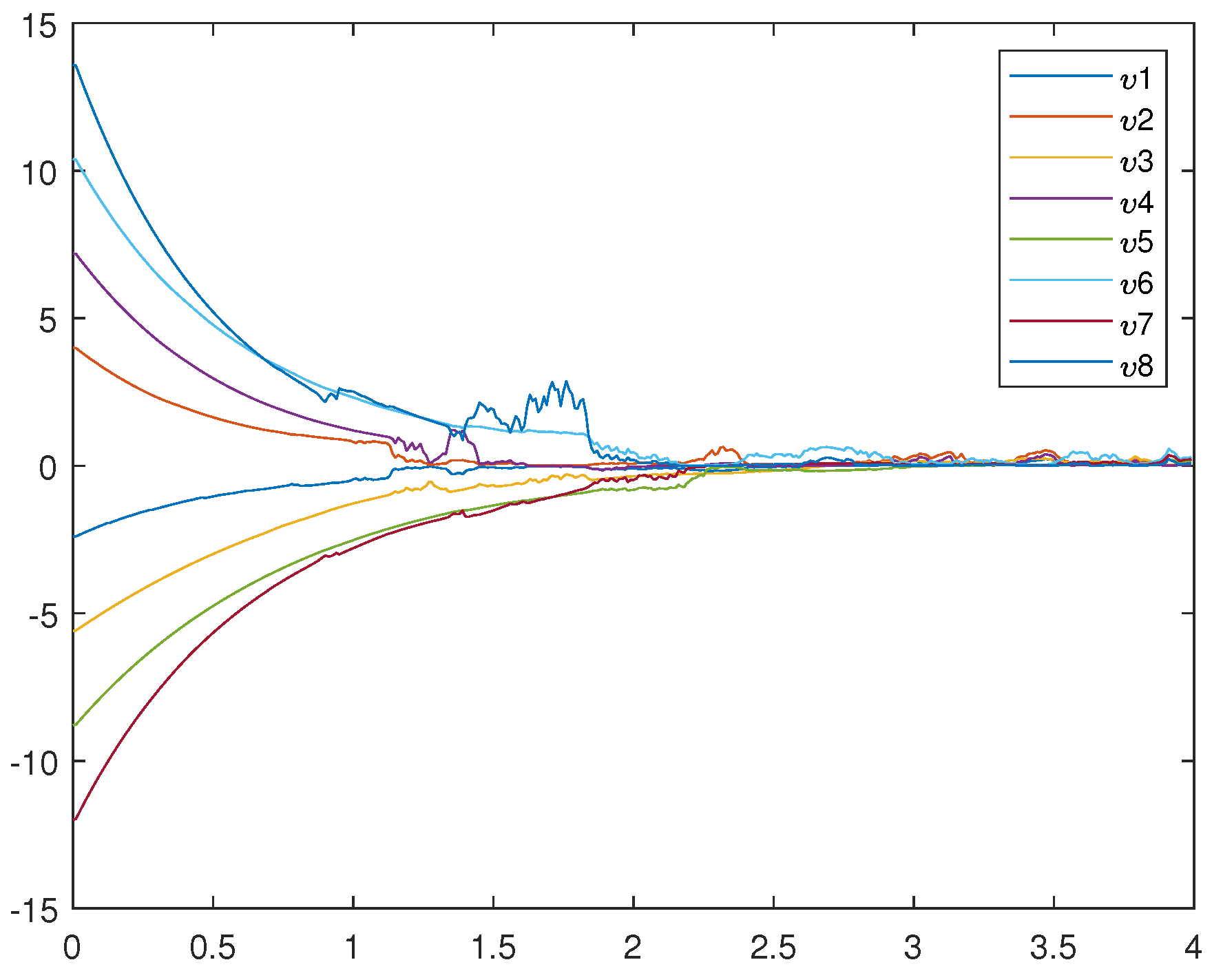
Figure 1. Trajectories of error system (14) without control ( u i ( t ) 0 ).
Axioms 13 00391 g001
Figure 2. Trajectories of drive system (12).
Axioms 13 00391 g002
Figure 3. Trajectories of response system (13) with feedback control (15).
Axioms 13 00391 g003
Figure 4. Trajectories of error system (14) with feedback control (15).
Axioms 13 00391 g004
Figure 5. Trajectories of drive system (12).
Axioms 13 00391 g005
Figure 6. Trajectories of response system (13) with adaptive control (16).
Axioms 13 00391 g006
Figure 7. Trajectories of error system (14) with adaptive control (16).
Axioms 13 00391 g007
Figure 8. Trajectories of drive system (18).
Axioms 13 00391 g008
Figure 9. Trajectories of response system (19) with adaptive control (17).
Axioms 13 00391 g009
Figure 10. Trajectories of error system (20) with adaptive control (17).
Axioms 13 00391 g010
Table 1. Values of k i j .
j12345678
k i j
i
10.420.510.620.410.450.4700.39
20.370.2400.380.3200.450
300.150.1700.200.290.280.42
40.1800.200.1900.160.190.20
50.2400.3100.2600.260
60.370.2900.2300.440.380.2
700.270.190.360.310.2800.40
80.280.310.220.290.280.320.300.23
Table 2. Values of d i j .
j12345678
d i j
i
10.600.520.620.650.600.590.700.49
20.600.470.630.560.620.660.490.66
30.500.630.510.690.640.550.510.65
40.600.680.640.5700.570.640.71
50.700.600.600.530.650.630.660.59
60.700.700.580.460.570.600.520.65
70.500.540.570.650.550.600.630.55
80.600.660.650.690.600.600.650.60
Table 3. Values of h i j .
j12345678
h i j
i
10.620.5600.620.600.590.700.49
200.470.6300.600.660.490.66
30.500.630.510.610.600.550.510.65
40.580.640.620.650.6500.640.71
50.7000.600.530.650.630.660.59
60.700.700.600.480.550.600.520.65
70.500.540.570.650.550.6000.55
80.600.660.650.670.600.600.650
Disclaimer/Publisher’s Note: The statements, opinions and data contained in all publications are solely those of the individual author(s) and contributor(s) and not of MDPI and/or the editor(s). MDPI and/or the editor(s) disclaim responsibility for any injury to people or property resulting from any ideas, methods, instructions or products referred to in the content.