An Optimization Problem for Computing Predictive Potential of General Sum/Product-Connectivity Topological Indices of Physicochemical Properties of Benzenoid Hydrocarbons

Abstract

For a graph $G=(V_G,E_G)$, a degree-based graphical index $G{I}_d$ takes the general form $G{I}_d={\displaystyle \sum _{xy\in E_G}}\varphi (d_x,d_y)$, where $\varphi$ is a symmetric map and $d_i$ is the degree of $i\in V_G$. For $\alpha \in \mathbb{R}$, if $\varphi ={\left(d_x{d}_y\right)}^{\alpha }$ (resp. $\varphi ={(d_x+d_y)}^{\alpha }$), the index is called the general product-connectivity $R_{\alpha }$ (resp. general sum-connectivity $SC{I}_{\alpha }$) index. In this paper, by formulating an optimization problem, we determine the value(s) of $\alpha$, for which the linear/multiple correlation coefficient of $R_{\alpha }$ and $SC{I}_{\alpha }$ with physicochemical properties of benzenoid hydrocarbons is the strongest. This, in turn, fills some research gaps left by similar studies in this area.

1. Introduction

Structure–property modeling employs molecular descriptors [1] to generate regression models correlating the physicochemical, biological, or thermodynamic properties of chemical compounds. Degree-based graphical indices are a class of graph-theoretic molecular descriptors that gained popularity in efficiently correlating the physicochemical properties of benzenoid hydrocarbons (BHs). In 1975, Randić introduced the connectivity index, commonly referred to as the Randić index (cf. [2]). Over the years, this index has emerged as the predominant molecular descriptor in Quantitative Structure–Property Relationship (QSPR) and Quantitative Structure–Activity Relationship (QSAR) studies (cf. [2]). Its mathematical properties have been extensively examined, as succinctly outlined in two recent monographs [2,3]. Moreover, various modifications and alternative formulations of this index have been proposed in the scientific literature (cf. [4,5]). In the present discourse, we also explore a closely affiliated variant of the connectivity index, denoted as the sum-connectivity index [6]. For some recent progress on the structure–property modeling of the physicochemical properties of nanostructures and bio-molecular networks, we refer to [7,8,9,10].

In order to test the quality of a certain class of molecular graphical descriptors, it is customary to conduct comparative testing by selecting suitable test molecules and their particular chemical properties. Gutman and Tošović [11] tested the quality of degree-dependent graphical descriptors for correlating the physicochemical properties of ismeric octanes (representatives of alkanes). Malik et al. [12] extended this study of degree-based molecular indices from octane-isomers to benzenoid hydrocarbons (BHs). Hayat et al. [13] (resp. Hayat et al. [14]) further extended the work from physicochemical properties to the quantum-theoretical (resp. thermodynamic) properties of BHs.

In their study, Gutman and Tošović [11] selected isomeric octanes as test molecules, whereas, other studies [11,12,14] opted for the lower 20–30 BHs as test molecules for their investigation. Moreover, Gutman and Tošović [11] and Malik et al. [12] selected the normal boiling point ($bp$) and the standard enthalpy of formation $\Delta H_f^o$ to represent physicochemical characteristics. Van der Waals and intermolecular forms of interactions are represented by $bp$, whereas, $\Delta H_f^o$ advocates for the thermal characteristics of a compound. On the other hand, the total $\pi$-electronic energy ($E_{\pi }$) was selected to represent quantum-theoretical characteristics by Hayat et al. [13] and the entropy and heat capacity were selected to advocate for thermodynamic properties by Hayat et al. [14].

All of the aforementioned quality testing revealed the strong potential of both general product-connectivity $R_{\alpha }$ and sum-connectivity $SC{I}_{\alpha }$ indices to efficiently correlate the physicochemical, thermodynamical, and quantum-theoretical characteristics of benzenoid hydrocarbons. For instance, Malik et al. [12] showed that, among all degree-based descriptors, $R_{-1}$ and $SC{I}_{-2}$ are the top two indices in correlating physicochemical characteristics of BHs. Similarly, Hayat et al. [13] showcased that $SC{I}_{-\frac{1}{2}}$ and $R_{-0.2661}$ are the best descriptors in predicting the $E_{\pi }$ of BHs, whereas Hayat et al. [14] showed that $SC{I}_{-3}$ and $R_{-1}$ are best two indices for correlating the thermodynamic properties of BHs. However, the disadvantage to these studies is that they consider both $R_{\alpha }$ and $SC{I}_{\alpha }$ in their comparative testing for only finite values of $\alpha$, i.e., $\alpha \in \left\{\pm \frac{1}{2}\pm 1,\pm 2\right\}$. Since both $R_{\alpha }$ and $SC{I}_{\alpha }$ deliver strong potential in correlating various properties of BHs, it is natural to consider these indices by considering the general $\alpha \in \mathbb{R}\setminus \left\{0\right\}$. Note that there might be a possibility that some other nonlinear function $\varphi (d_x,d_y)$, for instance considering other powers of $\alpha$, could work even better. However, the current study is restricted to investigating the estimation potential of $R_{\alpha }$ and $SC{I}_{\alpha }$ only.

In summary, current comparative studies considered $R_{\alpha }$ and $SC{I}_{\alpha }$ for $\alpha \in \left\{\pm \frac{1}{2}\pm 1,\pm 2\right\}$ and showed that both $R_{\alpha }$ and $SC{I}_{\alpha }$ with some of these values of $\alpha$ correlate well with the physicochemical properties as well as the total $\pi$-electron energy ($E_{\pi }$) of benzenoid hydrocarbons (BHs). For instance, Malik et al. [12] showed that $R_{-1}$ and $SC{I}_{-2}$ are the top two best degree-based predictors for correlating the physicochemical properties of BHs. Moreover, Hayat et al. [13] showed that $SC{I}_{-\frac{1}{2}}$ correlates well with the $E_{\pi }$ of BHs. The only limitation of these studies was that they considered $R_{\alpha }$ and $SC{I}_{\alpha }$ for $\alpha \in \left\{\pm \frac{1}{2}\pm 1,\pm 2\right\}$ only. So, if $R_{\alpha }$ and $SC{I}_{\alpha }$ deliver good predictors for these fixed integral values, both $R_{\alpha }$ and $SC{I}_{\alpha }$ might deliver even better predictors if we consider the general values of $\alpha \in \mathbb{R}\setminus \left\{0\right\}$.

In this paper, we determine the value(s) of $\alpha$ for which both $SC{I}_{\alpha }$ and $R_{\alpha }$ deliver strong predictive potential for the physicochemical properties of BHs. Multiple correlation and regression analyses were also conducted to find the best $\alpha$ for which the strongest multiple correlation is delivered both by $SC{I}_{\alpha }$ and $R_{\alpha }$ simultaneously. Following Gutman and Tošović [11], the physicochemical properties $bp$ and $\Delta H_f^o$ were selected as the test properties of BHs. Moreover, 22 lower BHs were selected as the test molecules as the public availability of the experimental values of $bp$ and $\Delta H_f^o$ is ensured for these test molecules. A computational method was used to calculate the $SC{I}_{\alpha }$ and $R_{\alpha }$ of these 22 BHs and then a detailed statistical analysis was conducted to find the suitable values of $\alpha$ for which both $SC{I}_{\alpha }$ and $R_{\alpha }$ deliver strong predictive potential.

2. Mathematical Preliminaries

For a chemical graph $G=(V_G,E_G)$, a degree-based graphical index $G{I}_d$ takes the general form $G{I}_d={\displaystyle \sum _{xy\in E_G}}\varphi (d_x,d_y)$, where $\varphi$ is a symmetric map and $d_i$ is the degree of $i\in V_G$. The product-connectivity index of G, proposed by Randić in [15] back in 1975, is one of the earliest degree-based graphical indices. Later on, the index was renamed as the Randić index. Mathematically, it takes $\varphi ={\left(d_x{d}_y\right)}^{-\frac{1}{2}}$ in $G{I}_d$. Thus, the product-connectivity descriptor $R\left(G\right)$ is defined as:

$$R\left(G\right)=G{I}_d,\mathrm{where}\varphi (d_x,d_y)=\frac{1}{\sqrt{d_x{d}_y}}$$

(1)

The diversity of its applicability in cheminformatics makes the Randić index one of most-studied structure graphical descriptors. For instance, its mathematical and chemical properties were extensively examined in [2,16,17,18,19].

Introduced by Zhou and Trinajstić [6], the sum-connectivity index is another degree-related molecular graphical descriptor. For a graph G, it considers $\varphi ={(d_x+d_y)}^{-\frac{1}{2}}$ in $G{I}_d$. Therefore, the sum-connectivity $SCI\left(G\right)$ of G has the defining structure:

$$SCI\left(G\right)=G{I}_d,\mathrm{where}\varphi (d_x,d_y)=\frac{1}{\sqrt{d_x+d_y}}$$

(2)

The reader is suggested [12,13,20,21] for further studies on both applicative and mathematical perspectives of the sum-connectivity index.

The successful applicability of the product-connectivity and sum-connectivity indices motivated researchers to consider variants of these descriptors. Perhaps, the most well-studied variants are the generalized variants of the product- and sum-connectivity indices. For $\alpha \in \mathbb{R}$, if $\varphi ={\left(d_x{d}_y\right)}^{\alpha }$ (resp. $\varphi ={(d_x+d_y)}^{\alpha }$), the index is called the general product-connectivity $R_{\alpha }$ (resp. general sum-connectivity $SC{I}_{\alpha }$) index. The general product-connectivity index was put forward by Bollobás and Erdös [4] in 1998 while generalizing the classical $R\left(G\right)$ index:

$$R_{\alpha }\left(G\right)=G{I}_d,\mathrm{where}\varphi (d_x,d_y)={\left(d_x{d}_y\right)}^{\alpha },$$

(3)

where $\alpha \in \mathbb{R}\setminus \left\{0\right\}$. There have been numerous contributions in the chemical and mathematical literature published on the general product-connectivity index, see, for example, [2,22,23,24,25].

Similarly, Zhou and Trinajstić [26] in 2010 proposed the general sum-connectivity index with the following defining structure:

$$SC{I}_{\alpha }\left(G\right)=G{I}_d,\mathrm{where}\varphi (d_x,d_y)={(d_x+d_y)}^{\alpha },$$

(4)

where $\alpha \in \mathbb{R}\setminus \left\{0\right\}$. A detailed mathematical treatment is reported in [27,28,29,30]. The application perspective of $SC{I}_{\alpha }$ is reported in Gutman and Tošović [11] and Hayat et al. [14]. Obviously,

$$\begin{array}{cc}\hfill R\left(G\right)& =R_{-0.5}\left(G\right)\hfill \\ \hfill SCI\left(G\right)& =SC{I}_{-0.5}\left(G\right)\hfill \end{array}$$

In the field of statistics, the correlation coefficient between two finite-mean random variables X and Y is defined to be ${\rho }_{XY}=cov(X,Y)/{\sigma }_X{\sigma }_Y\in [-1,1]$, where cov is the covariance function, and ${\sigma }_X$ and ${\sigma }_Y$ represent the standard deviations of the random variables X and Y, respectively. The correlation coefficient measures both the direction and strength of the linear relationship between a predictor Y and a response variable X. For a series of k measurements of these variables, denoted by $x_n$ and $y_n$$(n=1,2,\dots ,k)$, the value ${\rho }_{XY}$ is estimated by

$$r_{xy}=\frac{{\sum }_{n=1}^k(x_n-\overline{x})(y_n-\overline{y})}{\sqrt{{\sum }_{n=1}^k{(x_n-\overline{x})}^2}\sqrt{{\sum }_{n=1}^k{(y_n-\overline{y})}^2}},$$

(5)

where $\overline{x}=\frac{1}{k}{\sum }_{n=1}^k{x}_n$ and $\overline{y}=\frac{1}{k}{\sum }_{n=1}^k{y}_n$. Values of $|{\rho }_{XY}|$ closer to 1 indicate a strong linear relationship between X and Y.

The correlation coefficient is strongly linked to the concept of the linear regression of Y against X by assuming a regression line $Y=aX+b+ϵ$ where $ϵ$ represents random errors, and $\{a,b\in \mathbb{R}\}$ are coefficients to be estimated. The ordinary least squares method is typically employed, with closed-form solutions of the estimators $\widehat{a}$ and $\widehat{b}$ for a and b, respectively, being readily available and widely known. In particular, for this simple linear regression model, $\widehat{a}=r_{xy}{s}_y/s_x$, where $s_x$ and $s_y$ are the unbiased estimators of ${\sigma }_x$ and ${\sigma }_Y$, respectively, while $\widehat{b}=\overline{y}-\widehat{a}\overline{x}$. Evidently, the correlation is related to the slope of the regression line.

The standard error of fit and correlation coefficient are both key goodness-of-fit measures in regression analysis. The standard error of fit is defined as

$$s(Y,X)=\sqrt{\frac{1}{k-2}\sum _{n=1}^k{(y_n-y_n^{\prime })}^2}$$

(6)

where $y_n^{\prime }=\widehat{a}{x}_n+\widehat{b}$ (the regression line’s resulting predicted value). This quantifies how much the observed values deviate from the values predicted by the model. Using various types of mathematical or statistical software, they can be calculated.

The linear regression model can be extended to include multiple predictors, e.g., $X_1,\cdots ,X_p$. Suppose we have two predictors $X_1$ and $X_2$, we may define the multiple correlation measure between these predictors and a single response variable Y as follows:

$$R=\sqrt{\left(\begin{array}{cc}{r}_{x_{1}y}& r_{x_{2}y}\end{array}\right){\left(\begin{array}{cc}1& r_{x_1{x}_2}\\ r_{x_2{x}_1}& 1\end{array}\right)}^{-1}\left(\begin{array}{c}{r}_{x_{1}y}\\ r_{x_{2}y}\end{array}\right)}\in [0,1].$$

In the context of multiple linear regression, the quantity $R^2$ is usually referred to as the coefficient of determination. It is interpreted as the proportion of variability in the response variable Y that is accounted for by the predictor variables $X_1$ and $X_2$. The value R, thus, provides a measure of the correlation between the observed values of Y and the values predicted by the multiple linear regression model involving $X_1$ and $X_2$.

3. Materials and Methods

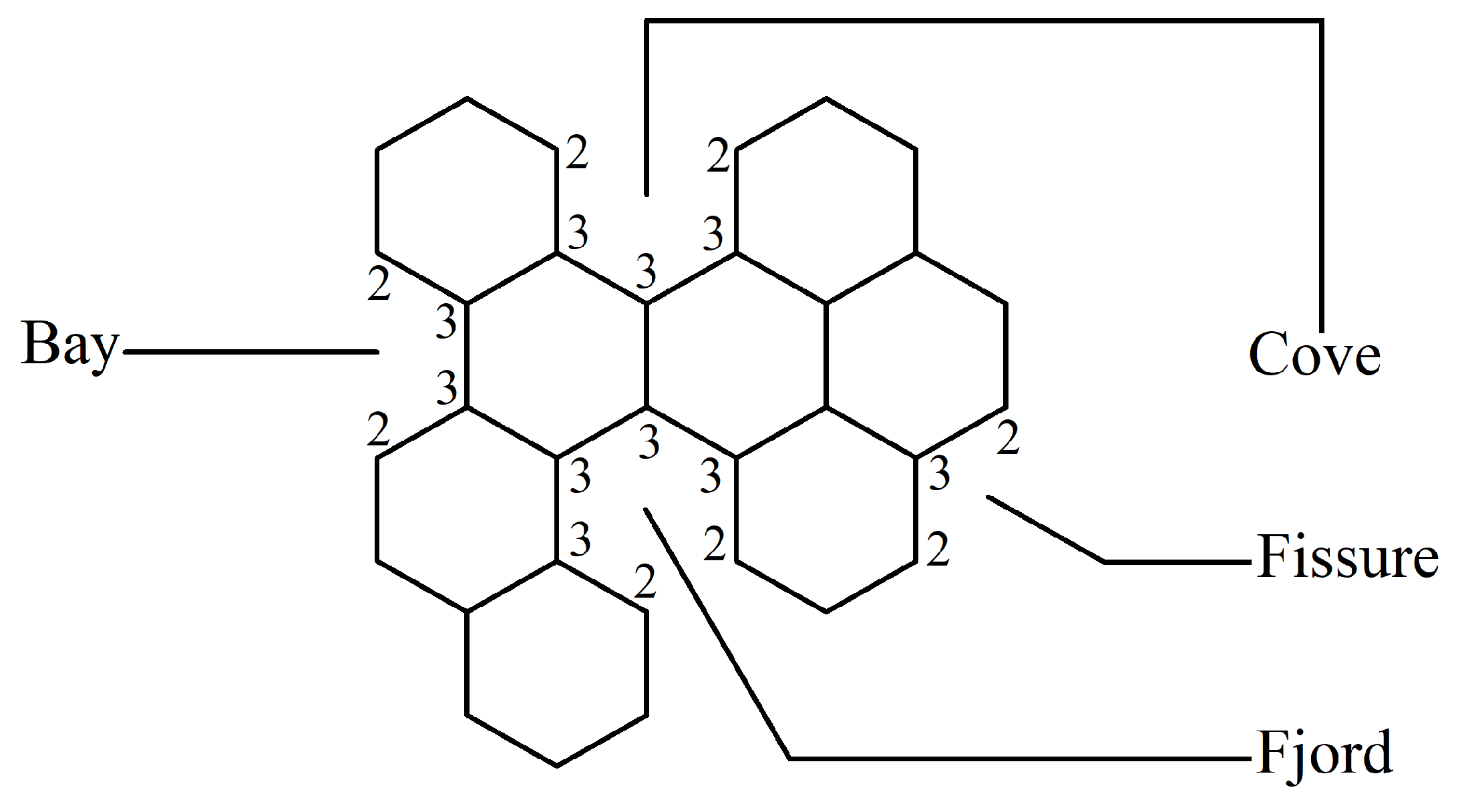
Every benzenoid hydrocarbon can be inherently depicted through a benzenoid system, defined as a finite, connected plane graph devoid of cut vertices, wherein each internal face is enclosed by a regular hexagon possessing sides of unit length.

The following definitions, as presented in [31], are applicable. Let B be a benzenoid system with v vertices and p hexagons. For any path $p_1-p_2-\cdots -p_{\ell +1}$ of length $\ell (\ell \in \mathbb{N},\ell \ge 1$) within B, the associated vertex degree sequence is defined as $(d_{p_1},d_{p_2},\dots ,d_{p_{\ell +1}})$. Subsequently, a fjord, cove, bay, and fissure refer to paths with degree sequences (2, 3, 3, 3, 3, 2), (2, 3, 3, 3, 2), (2, 3, 3, 2), and (2, 3, 2), respectively. These paths are traversed along the perimeter of B, as depicted in Figure 1. Fjords, coves, bays, and fissures are all considered different types of inlets. The number of inlets, k, is then defined as the total number of fjords, coves, bays, and fissures summed.

Suppose a benzenoid system B has p hexagons, k inlets, and v vertices. Let $n_{ij}$ denote the number of B’s edges that satisfies the conditions $d_a=i$ and $d_b=j$, where $d_a$ and $d_b$, respectively, are the degrees of the ends a and b of an edge. By Lemma 1 in [31], we have

$$n_{22}=v-2p-k+2,n_{23}=2k,n_{33}=3p-k-3.$$

(7)

By (3) and (7), the benzenoid system B has the general product-connectivity index as follows:

$$\begin{array}{cc}\hfill R_{\alpha }\left(B\right)& =n_{22}{4}^{\alpha }+n_{23}{6}^{\alpha }+n_{33}{9}^{\alpha }\hfill \\ \hfill & =\left(4^{\alpha }\right)v+(3·9^{\alpha }-2·4^{\alpha })p+(2·6^{\alpha }-4^{\alpha }-9^{\alpha })k-3·9^{\alpha }+2·4^{\alpha },\hfill \end{array}$$

(8)

By (4) and (7), the benzenoid system B has the general sum-connectivity index as follows:

$$\begin{array}{cc}\hfill SC{I}_{\alpha }\left(B\right)& =n_{22}{4}^{\alpha }+n_{23}{5}^{\alpha }+n_{33}{6}^{\alpha }\hfill \\ \hfill & =\left(4^{\alpha }\right)v+(3·6^{\alpha }-2·4^{\alpha })p+(2·5^{\alpha }-4^{\alpha }-6^{\alpha })k-3·6^{\alpha }+2·4^{\alpha },\hfill \end{array}$$

(9)

We employ (8) and (9) to compute the $R_{\alpha }$ and $SC{I}_{\alpha }$ for the 22 lower BHs given in

Table 1. The structural configuration of molecules, along with the experimental data pertaining to the standard enthalpy of formation ($\Delta H_f^o$) and the normal boiling point ($bp$), is provided for a set of 22 lower benzenoid hydrocarbons.

Molecule	Structure	$\mathit{\Delta }{\mathit{H}}_{\mathit{f}}^{\mathit{o}}$	$\mathit{bp}$
Benzene		75.2	80.1
Naphthalene		141	218
Phenanthrene		202.7	338
Anthracene		222.6	340
Chrysene		271.1	431
Benzo[a]anthracene		277.1	425
Triphenylene		275.1	429
Tetracene		310.5	440
Benzo[a]pyrene		296	496
Benzo[e]pyrene		289.9	493
Perylene		319.2	497
Anthanthrene		323	547
Benzo[ghi]perylene		301.2	542
Dibenzo[a,c]anthracene		348	535
Dibenzo[a,h]anthracene		335	535
Dibenzo[a,j]anthracene		336.3	531
Picene		336.9	519
Coronene		296.7	590
Dibenzo(a,h)pyrene		375.6	596
Dibenzo(a,i)pyrene		366	594
Dibenzo(a,l)pyrene		393.3	595
Pyrene		221.3	393

.

Table 1 provides information on the molecular structure, normal boiling point ($bp$), and standard enthalpy of formation ($\Delta H_f^o$) for various polycyclic aromatic hydrocarbons (PAHs). Additionally,

Table 2. The general product-connectivity index $R_{\alpha }$ and the general sum-connectivity index $SC{I}_{\alpha }$ of the 22 lower benzenoid hydrocarbons.

Molecule	${\mathit{R}}_{\mathit{\alpha }}$	${\mathit{SCI}}_{\mathit{\alpha }}$
Benzene	$6·4^{\alpha }$	$6·4^{\alpha }$
Naphthalene	$6·4^{\alpha }+4·6^{\alpha }+9^{\alpha }$	$6·4^{\alpha }+4·5^{\alpha }+6^{\alpha }$
Phenanthrene	$7·4^{\alpha }+6·6^{\alpha }+3·9^{\alpha }$	$7·4^{\alpha }+6·5^{\alpha }+3·6^{\alpha }$
Anthracene	$6·4^{\alpha }+8·6^{\alpha }+2·9^{\alpha }$	$6·4^{\alpha }+8·5^{\alpha }+2·6^{\alpha }$
Chrysene	$8·4^{\alpha }+8·6^{\alpha }+5·9^{\alpha }$	$8·4^{\alpha }+8·5^{\alpha }+5·6^{\alpha }$
Benzo[a]anthracene	$7·4^{\alpha }+10·6^{\alpha }+4·9^{\alpha }$	$7·4^{\alpha }+10·5^{\alpha }+4·6^{\alpha }$
Triphenylene	$9·4^{\alpha }+6·6^{\alpha }+6·9^{\alpha }$	$9·4^{\alpha }+6·5^{\alpha }+6·6^{\alpha }$
Tetracene	$6·4^{\alpha }+12·6^{\alpha }+3·9^{\alpha }$	$6·4^{\alpha }+12·5^{\alpha }+3·6^{\alpha }$
Benzo[a]pyrene	$7·4^{\alpha }+10·6^{\alpha }+7·9^{\alpha }$	$7·4^{\alpha }+10·5^{\alpha }+7·6^{\alpha }$
Benzo[e]pyrene	$8·4^{\alpha }+8·6^{\alpha }+8·9^{\alpha }$	$8·4^{\alpha }+8·5^{\alpha }+8·6^{\alpha }$
Perylene	$8·4^{\alpha }+8·6^{\alpha }+8·9^{\alpha }$	$8·4^{\alpha }+8·5^{\alpha }+8·6^{\alpha }$
Anthanthrene	$6·4^{\alpha }+12·6^{\alpha }+9·9^{\alpha }$	$6·4^{\alpha }+12·5^{\alpha }+9·6^{\alpha }$
Benzo[ghi]perylene	$7·4^{\alpha }+10·6^{\alpha }+10·9^{\alpha }$	$7·4^{\alpha }+10·5^{\alpha }+10·6^{\alpha }$
Dibenzo[a,c]anthracene	$9·4^{\alpha }+10·6^{\alpha }+7·9^{\alpha }$	$9·4^{\alpha }+10·5^{\alpha }+7·6^{\alpha }$
Dibenzo[a,h]anthracene	$8·4^{\alpha }+12·6^{\alpha }+6·9^{\alpha }$	$8·4^{\alpha }+12·5^{\alpha }+6·6^{\alpha }$
Dibenzo[a,j]anthracene	$8·4^{\alpha }+12·6^{\alpha }+6·9^{\alpha }$	$8·4^{\alpha }+12·5^{\alpha }+6·6^{\alpha }$
Picene	$9·4^{\alpha }+10·6^{\alpha }+7·9^{\alpha }$	$9·4^{\alpha }+10·5^{\alpha }+7·6^{\alpha }$
Coronene	$6·4^{\alpha }+12·6^{\alpha }+12·9^{\alpha }$	$6·4^{\alpha }+12·5^{\alpha }+12·6^{\alpha }$
Dibenzo(a,h)pyrene	$8·4^{\alpha }+12·6^{\alpha }+9·9^{\alpha }$	$8·4^{\alpha }+12·5^{\alpha }+9·6^{\alpha }$
Dibenzo(a,i)pyrene	$8·4^{\alpha }+12·6^{\alpha }+9·9^{\alpha }$	$8·4^{\alpha }+12·5^{\alpha }+9·6^{\alpha }$
Dibenzo(a,l)pyrene	$9·4^{\alpha }+10·6^{\alpha }+10·9^{\alpha }$	$9·4^{\alpha }+10·5^{\alpha }+10·6^{\alpha }$
Pyrene	$6·4^{\alpha }+8·6^{\alpha }+5·9^{\alpha }$	$6·4^{\alpha }+8·5^{\alpha }+5·6^{\alpha }$

presents data on the general product-connectivity index $R_{\alpha }$ and the general sum-connectivity index $SC{I}_{\alpha }$ for the 22 lower BHs.

4. Results and Discussion

Recall that the general product-connectivity index $R_{\alpha }$ and the general sum-connectivity index $SC{I}_{\alpha }$ considering a range of values $\alpha$ exhibit a high degree of accuracy in predicting the boiling point and enthalpy of formation for the lower benzenoid hydrocarbons (BHs).

First, we employed the method described in Section 3 to evaluate the exact analytical expressions for $R_{\alpha }$ and $SC{I}_{\alpha }$ for the 22 lower BHs provided in Table 1. In particular, we utilized expressions for $R_{\alpha }$ and $SC{I}_{\alpha }$ in (8) and (9), respectively, to compute their exact values. Note that, we only needed the number of vertices v, the number of inlets k, and the number of hexagons p for a given hexagonal system to compute its $R_{\alpha }$ and $SC{I}_{\alpha }$ values. The next example explains the methodology in Section 3 to compute the general sum- and product-connectivity indices for a given BH graph.

Example  1. 

Let us consider the graph of phenanthrene, e.g., P from Table 1. Then, P comprises two fissures, one bay (three inlets in total), three hexagons, and 14 vertices. Thus, $v=14$, $k=3$, and $p=3$. Using these values in (8) and (9), we obtain:

$$\begin{array}{ccc}\hfill R_{\alpha }\left(P\right)& =& 7·4^{\alpha }+6·6^{\alpha }+3·9^{\alpha }\hfill \\ \hfill SC{I}_{\alpha }\left(P\right)& =& 7·4^{\alpha }+6·5^{\alpha }+3·6^{\alpha }.\hfill \end{array}$$

By using this method for all the graphs in Table 1, we generated the data in Table 2.

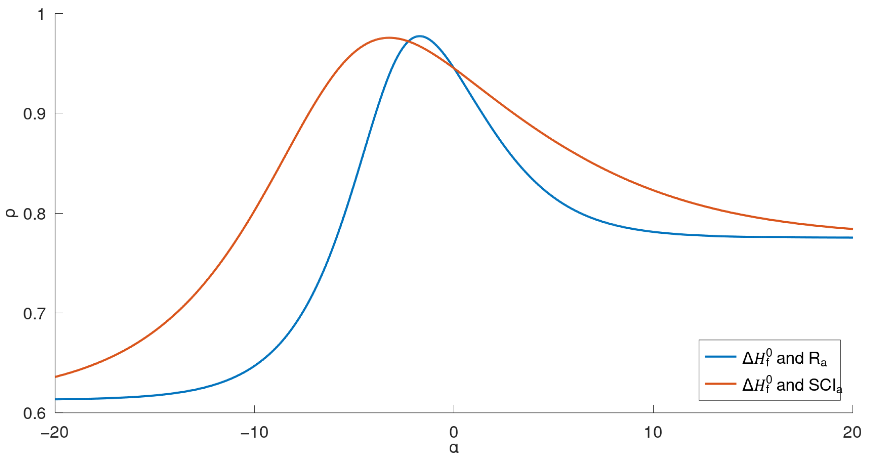
From the data shown in Table 2, we generated four curves, as illustrated in Figure 2, Figure 3, Figure 4 and Figure 5. For these 22 lower BHs, the correlation coefficient curves for their physicochemical properties ($bp$ in Figure 2 and Figure 3; $\Delta H_f^0$ in Figure 4 and Figure 5) and the indices ($R_{\alpha }$ or $SC{I}_{\alpha }$) are drawn in the respective figures in solid lines, distinguished by colors.

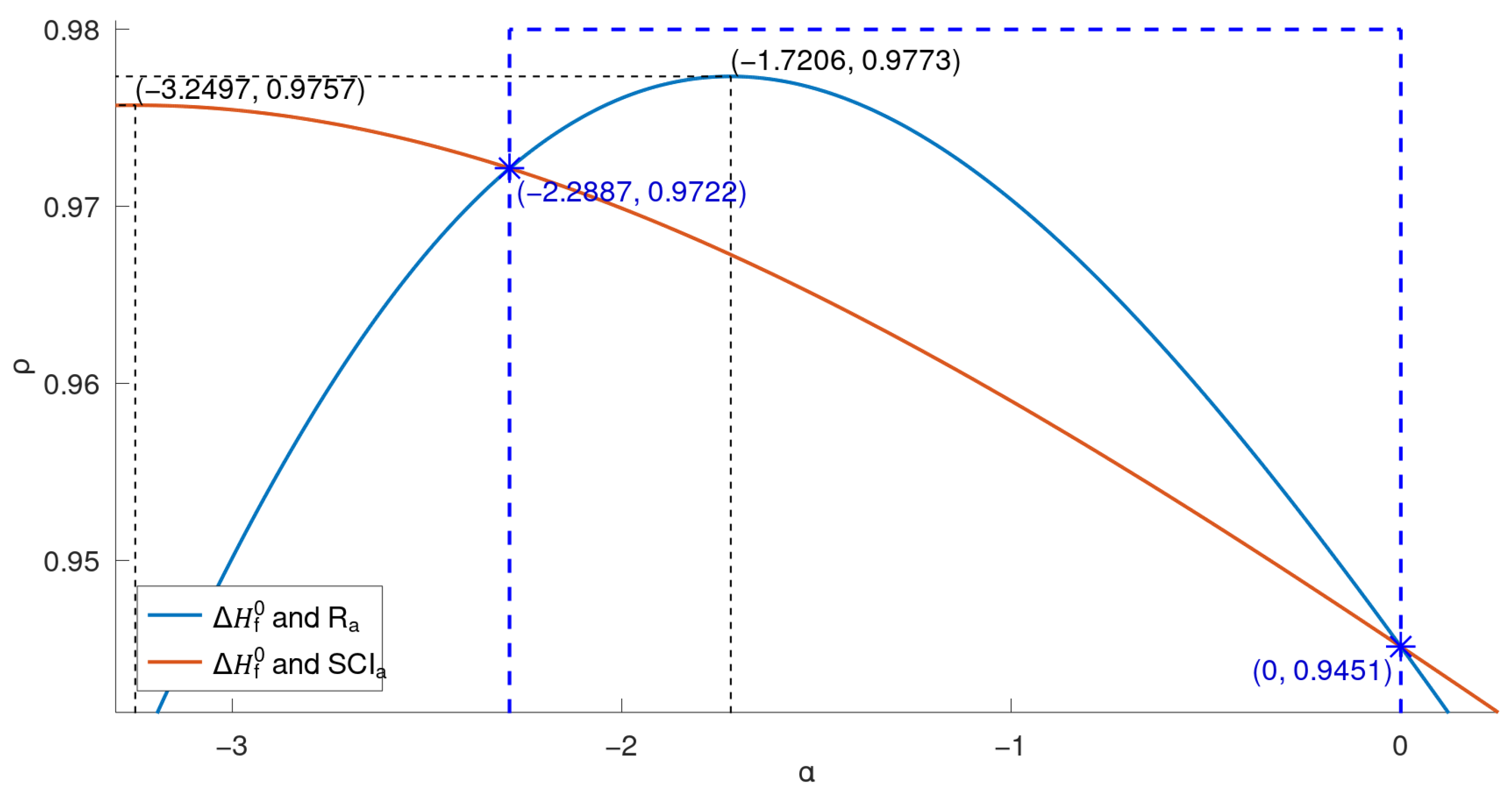
Comparing the two general indices, the general product-connectivity index $R_{\alpha }$ is the best measure of the boiling point $bp$ for BHs for $\alpha \in (-0.4630,0)$, as shown in Figure 3, while for any other $\alpha$, the sum-connectivity index $SC{I}_{\alpha }$ is the best. On the other hand, as measures of the enthalpy of formation $\Delta H_f^o$ of benzenoid hydrocarbons, the general product-connectivity index $R_{\alpha }$ is better for $\alpha \in (-2.2887,0)$, as can be seen in Figure 5, while for any other $\alpha$, the sum-connectivity index $SC{I}_{\alpha }$ is better.

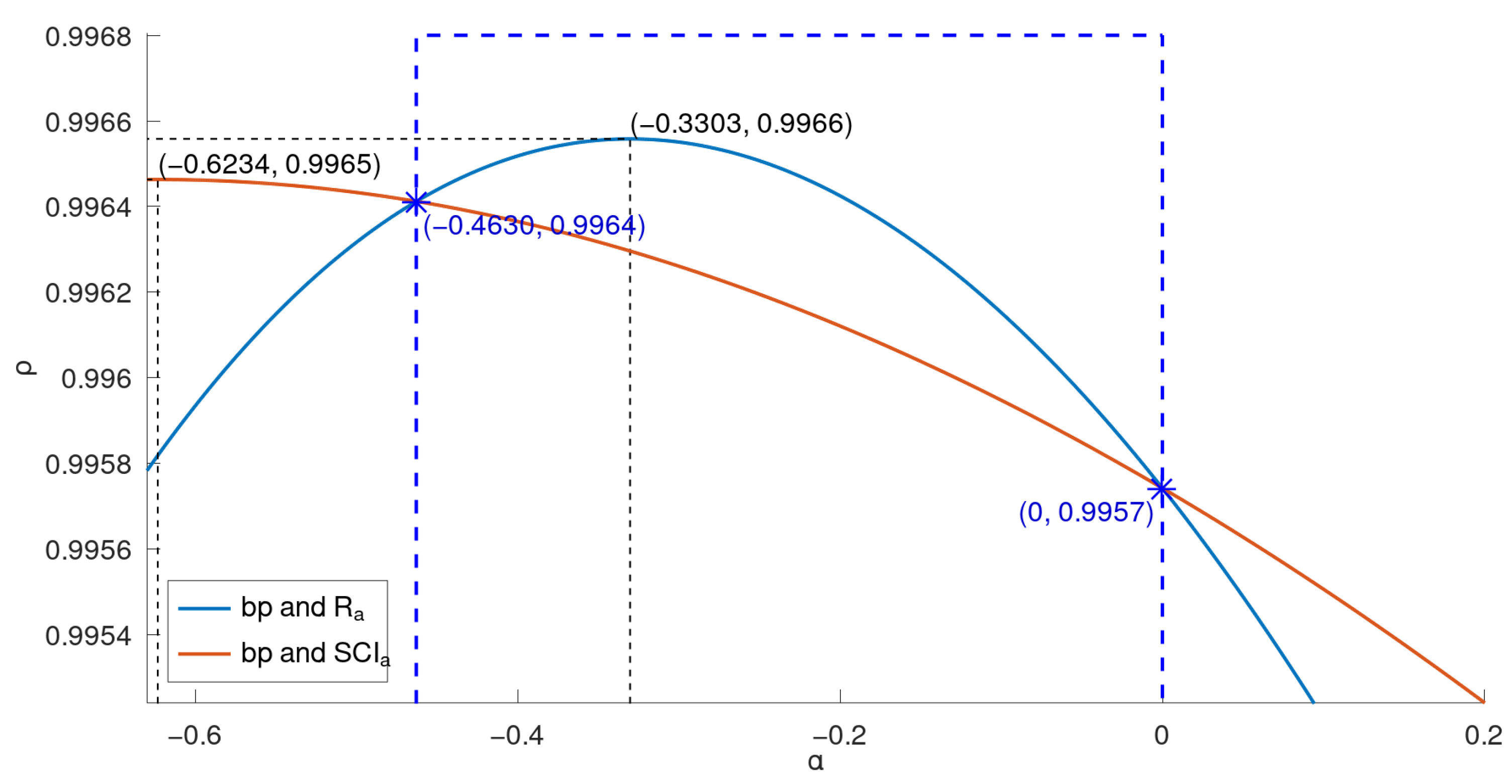
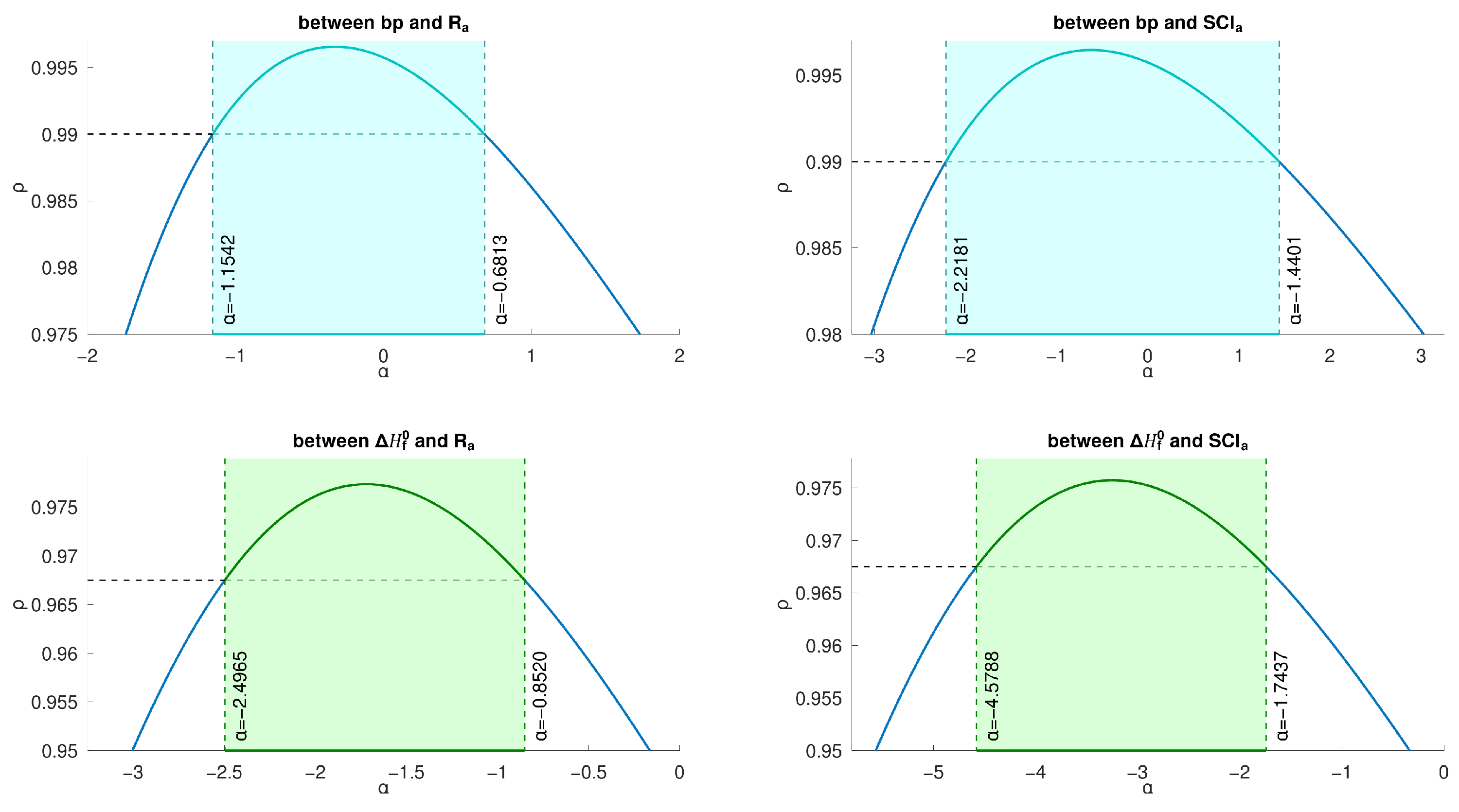
There exists a good correlation between $bp$ and $R_{\alpha }$ when $\alpha$ is in some interval. For example, for $\alpha \in [-1.154217,0.681350]$, $bp$ and $R_{\alpha }$ have a correlation coefficient greater than 0.996558. Similarly, there also exists—for $\alpha$ in different intervals—a good correlation between $bp$ and $SC{I}_{\alpha }$, between $\Delta H_f^0$ and $R_{\alpha }$, and between $\Delta H_f^0$ and $SC{I}_{\alpha }$, as shown in Figure 6.

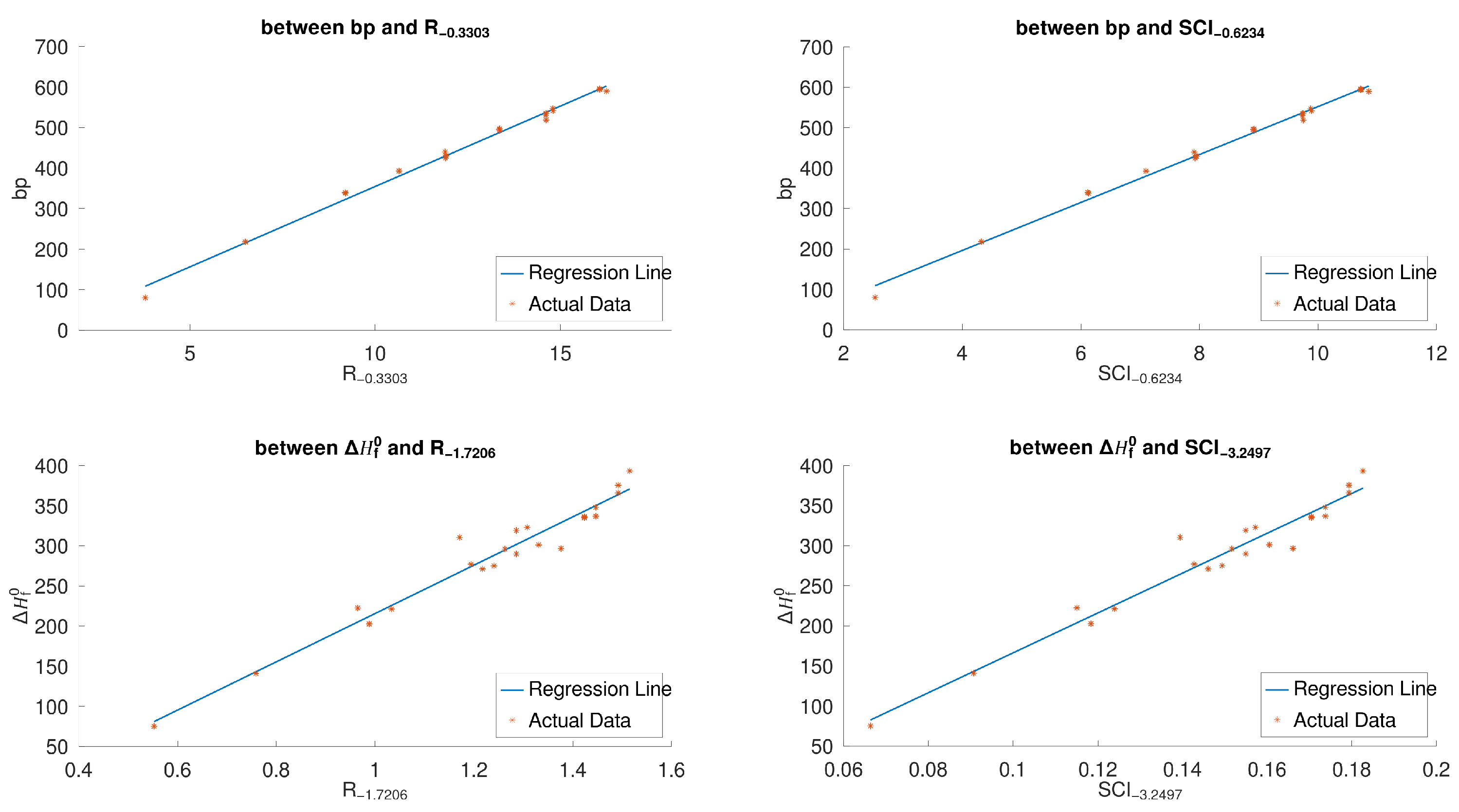
By Figure 3 and Figure 5, we have that, for the 22 lower BHs, $R_{-0.3303}$ and $R_{-1.7205}$ are the most linearly correlated with $bp$ and $\Delta H_f^0$, respectively, among all product-connectivity indices, and $SC{I}_{-0.6233}$ and $SC{I}_{-3.2496}$ are the most linearly correlated with $bp$ and $\Delta H_f^0$, respectively, among all sum-connectivity indices. The linear correlations (with 95% confidence intervals) between the physicochemical properties ($bp$ and $\Delta H_f^0$) and both of the aforementioned indices, respectively, are given below:

$$\begin{array}{cc}\hfill & bp=39.{693}_{\pm 1.540}-42.{183}_{\pm 20.161}{R}_{-0.33030},\hfill \\ \hfill \rho (& bp,R_{-0.33030})=0.996558,s(bp,R_{-0.33030})=10.9571,\hfill \end{array}$$

(10)

$$\begin{array}{cc}\hfill & bp=59.{430}_{\pm 2.334}-40.{884}_{\pm 20.388}SC{I}_{-0.62336},\hfill \\ \hfill \rho (& bp,SC{I}_{-0.62336})=0.996463,s(bp,SC{I}_{-0.62336})=11.1067,\hfill \end{array}$$

(11)

$$\begin{array}{cc}\hfill \Delta & H_f^0=300.{943}_{\pm 30.399}-85.{181}_{\pm 38.305}{R}_{-1.72056},\hfill \\ \hfill \rho (\Delta & H_f^0,R_{-1.72056})=0.977344,s(\Delta H_f^0,R_{-1.72056})=16.5206,\hfill \end{array}$$

(12)

$$\begin{array}{cc}\hfill \Delta & H_f^0=2486.{468}_{\pm 260.362}-82.{232}_{\pm 39.402}SC{I}_{-3.24966},\hfill \\ \hfill \rho (& E,SC{I}_{-3.24966})=0.975715,s(E,SC{I}_{-3.24966})=17.0968,\hfill \end{array}$$

(13)

Note that s and $\rho$ are the standard error of fit and correlation coefficient, respectively. Figure 7 shows scatter plots between the boiling point $bp$ and the indices $R_{-0.33030}$ and $SC{I}_{-0.62336}$, and scatter plots between the enthalpy of formation $\Delta H_f^0$ and the indices $R_{-1.72056}$ and $SC{I}_{-3.24966}$ for the 30 lower benzenoids.

It is obvious from (10)–(13) that the product-connectivity indices $R_{-0.33030}$ and $R_{-1.72056}$, respectively, are the best for measuring the boiling point and enthalpy of formation among all the examined indices. All the Octave codes have been made publicly accessible. See the Supplimentary Information at the end of the paper.

Recall that Gutman and Tošović [11] considered $bp$ and $\Delta H_f^0$ to be representatives of physicochemical properties. Moreover, they considered isomeric octanes as test molecules. We applied our study on the 18 isomeric octanes and the preliminary results showed that the value(s) of $\alpha$ for the 22 lower BHs yielding a good estimate of $bp$ and $\Delta H_f^0$ were not the same as they were for isomeric octanes. Thus, the current study and the corresponding intervals/values of $\alpha$ are limited to BHs only. However, we expect a similar behavior for other BHs (different from the 22 lower BHs considered in this study) as well.

5. Simultaneous Predictive Potential of ${\mathbf{R}}_{\mathbf{\alpha }}$ and ${\mathbf{SCI}}_{\mathbf{\alpha }}$

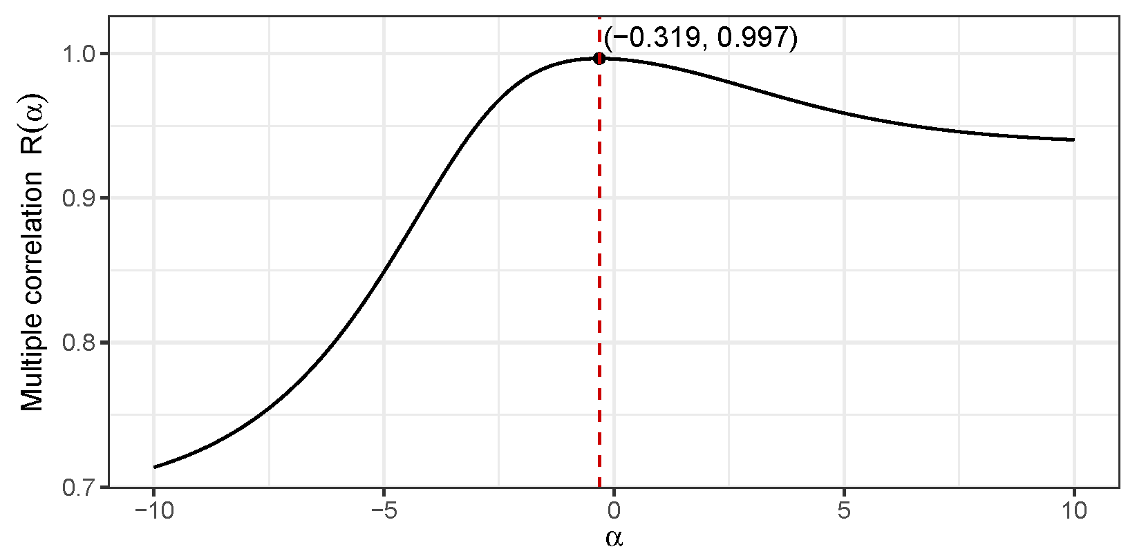
In this section, we are interested in finding value(s) of $\alpha$ for which the correlation of either $R_{\alpha }$ or $SC{I}_{\alpha }$ with both properties $bp$ and $\Delta H_f^o$ simultaneously is the strongest. In order to achieve that, we need to consider the multiple correlation coefficient of either $R_{\alpha }$ or $SC{I}_{\alpha }$ with both $bp$ and $\Delta H_f^o$ by treating them as two independent variables. Let $Y=R_{\alpha }$ be the dependent variable and $X_1=bp,X_2=\Delta H_f^o$ be the two independent variables. Note that the multiple correlation determines the relationship with one dependent and more than one independent variable. Since there are two representatives of physicochemical properties, i.e., $bp$ and $\Delta H_f^o$, we employ multiple correlation between one graphical descriptor $G{I}_d\in \{R_{\alpha },SC{I}_{\alpha }\}$ and the two chosen properties $X_1=bp,X_2=\Delta H_f^o$. This was able to deliver the predictive potential of a descriptor with the two properties simultaneously rather than determining the correlation strength of the considered descriptor with both properties individually.

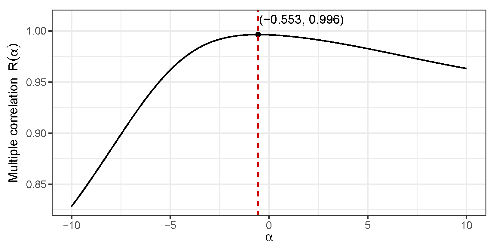
In the case where the response variable y depends on an unknown parameter $\alpha \in \mathbb{R}$, the value of multiple correlation $\rho$ above also depends on $\alpha$, i.e., $\rho :=\rho \left(\alpha \right)$. A preliminary plot of $\rho \left(\alpha \right)$ in the region $-10<\alpha <10$ reveals a unimodal shape with a maxima in this region. A built-in optimizer in the R programming language was employed that yielded the value $\widehat{\alpha }=-0.319$ that maximizes the multiple correlation value $\rho \left(\widehat{\alpha }\right)=0.997$. Figure 8 presents the corresponding plot elaborating this calculation.

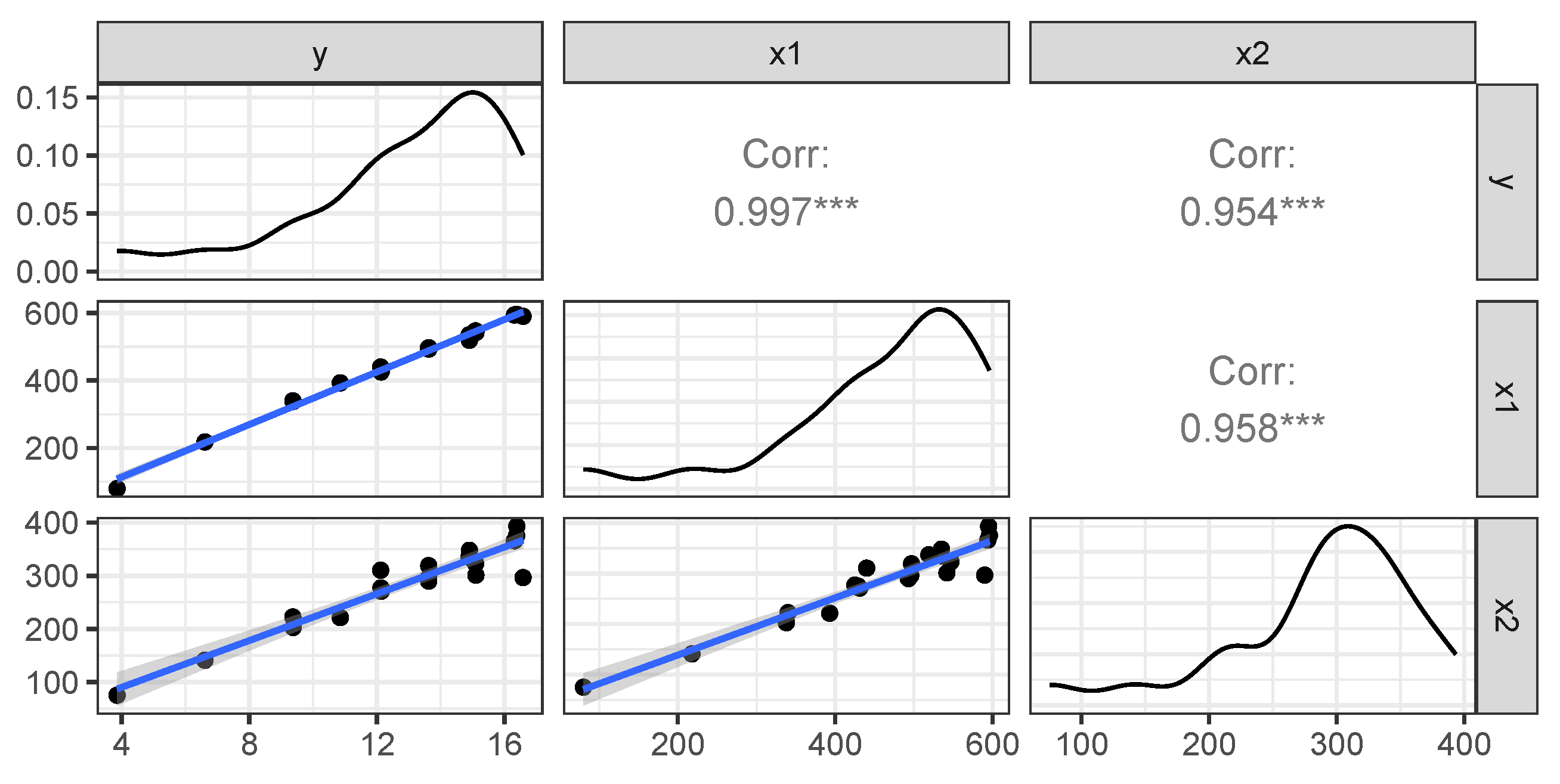
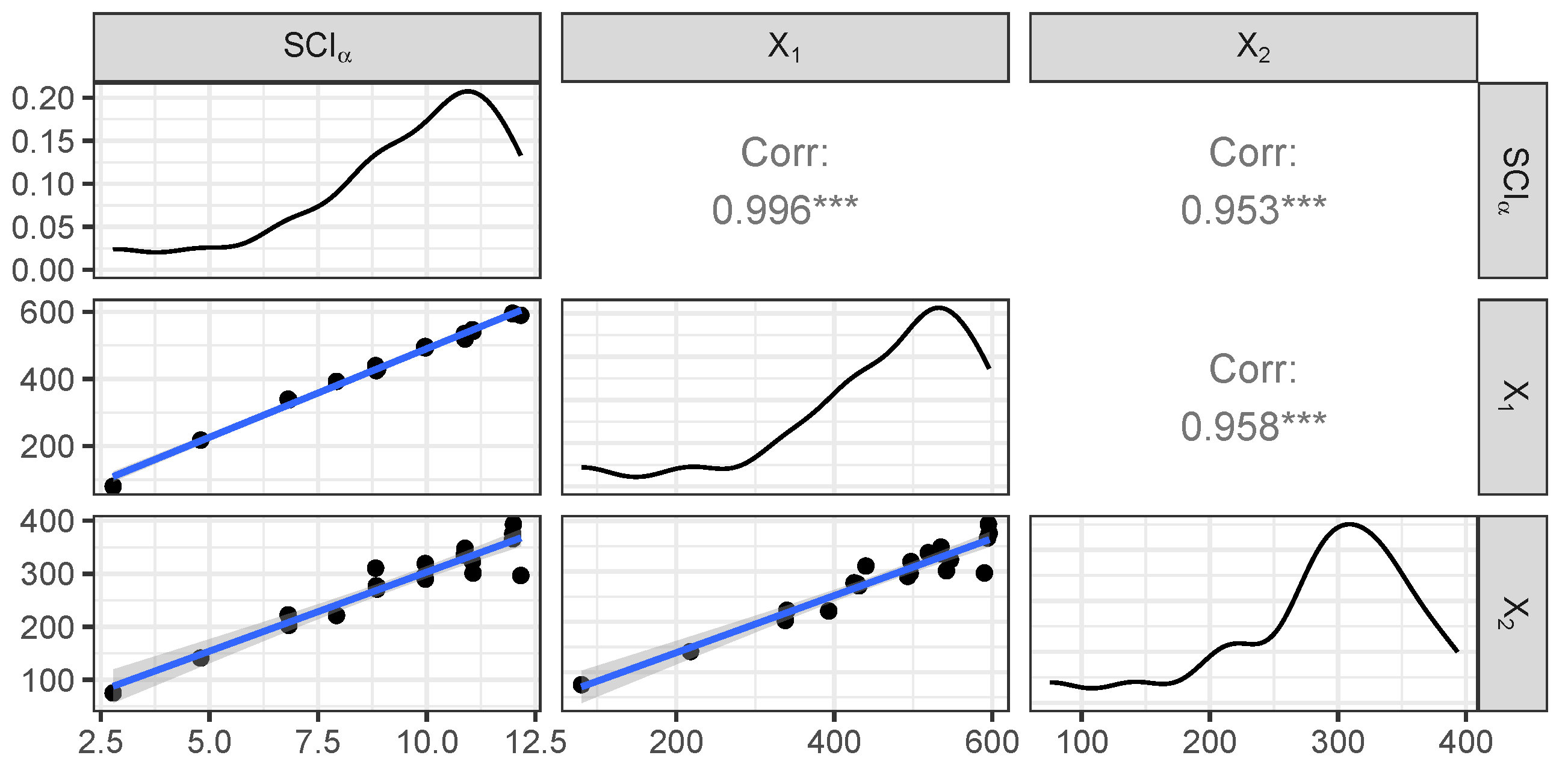
Figure 9 exhibits the matrix plot showing the distribution of the variables as well as the bivariate relationships between them (using the optimal value $\widehat{\alpha }$).

Next, we study the multiple correlation $\rho :=\rho \left(\alpha \right)$ between $Y=SC{I}_{\alpha }$ and the two chosen physicochemical properties $X_1=bp,X_2=\Delta H_f^o$. In the case where the response variables y depends on an unknown parameter $\alpha \in \mathbb{R}$, the value of R above also depends on $\alpha$, i.e., $\rho :=\rho \left(\alpha \right)$. A preliminary plot of $\rho \left(\alpha \right)$ in the region $-10<\alpha <10$ again reveals a unimodal shape with a maxima in this region. This time, the built in R optimizer yielded the value $\widehat{\alpha }=-0.553$, so $\rho \left(\widehat{\alpha }\right)=0.996$. Figure 10 presents the corresponding plot elaborating these values.

Figure 11 exhibits the matrix plot, showing the distribution of the variables as well as the bivariate relationships between them (using the optimal value $\widehat{\alpha }$).

6. Conclusions

We showed in this paper that there is good correlation between the boiling point ($bp$) and general product-connectivity index ($R_{\alpha }$), between $bp$ and the general sum-connectivity index ($SC{I}_{\alpha }$), between the enthalpy of formation ($\Delta H_f^0$) and $R_{\alpha }$, and between $\Delta H_f^0$ and $SC{I}_{\alpha }$ when $\alpha$ is in some intervals (as in Figure 6) for benzenoid hydrocarbons. Moreover, for $\alpha \in (-0.4630,0)$ and $\alpha \in (-2.2887,0)$ (marked with blue dashed lines in Figure 3 and Figure 5), $R_{\alpha }$ rather than $SC{I}_{\alpha }$ is a better measure of the boiling point and enthalpy of formation, respectively, of G. For an $\alpha$ outside those intervals, $SC{I}_{\alpha }$ is a better measure of both the boiling point and enthalpy of formation of G.

7. Future Work

This paper examined the correlation power of the general product-connectivity index and general sum-connectivity index to determine the boiling point ($bp$) of benzenoid hydrocarbons, and their correlation power to determine the enthalpy of formation ($\Delta H_f^0$) of benzenoid hydrocarbons. We propose further studies to similarly examine other generalized valency-based indices in determining the $bp$ and $\Delta H_f^0$ of benzenoid hydrocarbons. We also propose the following open problem:

Problem  2. 

Can one use a learning technique to learn a nonlinear function $\varphi (d_x,d_y)$ of minimal complexity that is a best predictor of $G{I}_d$?