Explicit Numerical Manifold Characteristic Galerkin Method for Solving Burgers’ Equation

Abstract

This paper presents a nonstandard numerical manifold method (NMM) for solving Burgers’ equation. Employing the characteristic Galerkin method, we initially apply the Crank–Nicolson method for temporal discretization along the characteristic. Subsequently, utilizing the Taylor expansion, we transform the semi-implicit formula into a fully explicit form. For spacial discretization, we construct the NMM dual-cover system tailored to Burgers’ equation. We choose constant cover functions and first-order weight functions to enhance computational efficiency and exactly import boundary constraints. Finally, the integrated computing scheme is derived by using the standard Galerkin method, along with a Thomas algorithm-based solution procedure. The proposed method is verified through six benchmark numerical examples under various initial boundary conditions. Extensive comparisons with analytical solutions and results from alternative methods are conducted, demonstrating the accuracy and stability of our approach, particularly in solving Burgers’ equation at high Reynolds numbers.

1. Introduction

As a fundamental nonlinear convection-diffusion equation, Burgers’ equation, named after Johannes M. Burgers [1], takes its form by simplifying the Navier–Stokes (N-S) equations while retaining the convection and viscosity terms. This model provides valuable insights into the behavior of complex waves occurring in turbulence, gas dynamics, nonlinear acoustics, traffic flow, etc. When the convection term tends to zero, Burgers’ equation becomes a quasi-linear hyperbolic conservation law, in which shock waves can develop in a limited time even using smooth enough initial conditions. Owing to its simplicity in form and ability to generate strong discontinuities, plenty of studies have been conducted to find out its approximate and analytical solutions under various initial and boundary conditions.

In contrast, the quasi-linear convection term in Burgers’ equation brings difficulty to numerical solution approaches. When the viscosity term diminishes as the Reynolds number increases, Burgers’ equation becomes convective dominant and results in steep wave fronts. In this case, numerical solutions often exhibit spurious oscillations around the discontinuities. Much effort has been dedicated to designing accurate and stable computing schemes to solve Burger’s equation for large Reynolds numbers. According to the manner for spacial discretization, these schemes can be roughly categorized into mesh-based approaches [2,3,4,5,6,7,8] and mesh-free methods [9,10]. However, mesh-based approaches, such as finite difference/volume/element methods, seriously rely on deliberated meshes to discretize problem domain onto grid lines or elements to acquire accurate spacial approximation.

Compared with mesh-based approaches, mesh-free methods offer flexibility and advantages in problems involving complex geometries, moving boundaries, discontinuities and sharp gradient issues. The core idea of mesh-free methods is to use scattered nodes or points to discrete the domain of interest in space rather than predefined meshes. In this way, the solution to partial differential equations can be approximated by interpolation or functionals at these nodes. In recent years, several mesh-free approaches have emerged and are increasingly applied to solve Burgers’ equation, such as the element-free Galerkin method [11,12], reproducing kernel particle method [13,14], and finite point method [15].

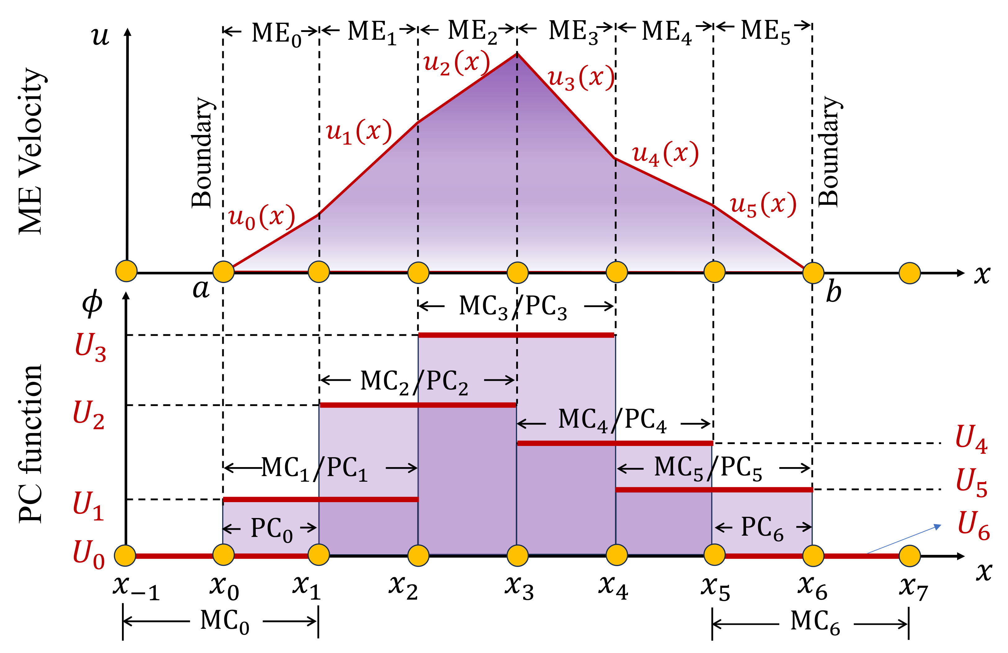
Numerical manifold method (NMM) [16] is a widely used computational approach for modeling large deformations [17], contacts [18] and fracture problems [19] in geotechnical engineering. The fundamental concept of the NMM is its dual-cover system for spacial discretization. Such a system is comprised of mathematical covers (MCs) and physical covers (PCs): MCs are a series of individual overlapping regions that occupy the whole material field, and PCs are subsequently generated by trimming MCs with material boundaries. The intersections of PCs form manifold elements (MEs), which connect PCs to reconstruct the entire problem domain. In the NMM, the approximation and integral are implemented on the PC and ME, respectively. The global approximation throughout the material domain is the assemblage of local cover functions by using the technique analogous to the partition-of-unity (PU) strategy. In this way, cover functions and weight functions can be chosen independently, and discontinuous global approximation is admissible. Such spacial discretization brings specific benefits for modeling problems involving complex geometry shapes and boundary conditions, such as moving boundaries and internal discontinuities.

Recently, the NMM has been applied to simulate more general problems, such as heat conduction Equations [20,21,22], incompressible N-S Equations [23] and seepage flows [24,25]. In those studies, the NMM shows substantial flexibility owing to its unique dual-cover system. Different from mesh-based approaches, the NMM can generate MCs through FE-type meshes, unstructured meshes and even the mesh with irregular shapes. Since MC meshes are not necessary to exactly coincide with the problem boundary, the pre-processing of the NMM is far simpler than mesh-based approaches. In this way, a lot of time can be saved. The solution obtained by the NMM can be $C^0$ functions and even contain discontinuous. Due to a larger admissible solution space, this method possesses more efficiency and stability. Compared with other mesh-free methods, the NMM uses polynomial cover approximation and weights but not complex deliberated functions. In such a manner, the integrals over MEs can be exactly calculated instead of using Gaussian quadrature.

In view of the aforementioned advantages of the NMM, we present a new NMM scheme, referred to as the explicit numerical manifold characteristic Galerkin method (ENMCGM), to numerically solve Burgers’ equation in the present work.

Regarding temporal discretization, we use the Crank–Nicolson method (CNM) to transfer the equation into a finite difference form along the characteristic firstly and then adopt Taylor expansion and convert it into an explicit semi-discretization scheme. No extra parameter is introduced to ensure computation convergence.

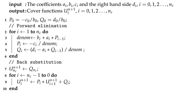
Regarding spacial discretization, we obtain the weak form of the semi-discretization of Burgers’ equation by using the standard Galerkin method first and then integrate the formulation by parts and obtain the presented scheme. Furthermore, we adopt the Thomas algorithm to solve the resulting tridiagonal linear equations, and iterative formulations are derived in detail. As an explicit method, the ENMCGM is conditionally stable. We give an estimation for the time step size of our method based on the CFL condition.

Plenty of numerical examples are conducted to validate the proposed method for varied initial conditions and boundary conditions as well as varying Reynolds numbers. We evaluated the results by contrasting them with analytical solutions and findings obtained from alternative methods. Comparisons demonstrate that the proposed ENMCGM is accurate and stable, even for large Reynolds numbers. The outline of this paper is arranged as follows. Section 2 presents an introduction to the Burgers’ equation. In Section 3, the temporal discretization is carried out. Section 4 provides the dual-cover-based approximation for the velocity. Section 5 presents the spacial discretization of Burgers’ equation and the integrated computing scheme of the ENMCGM. In Section 6, numerical examples are conducted to evaluate the presented method, and the conclusion of this paper comes in Section 7.

2. Burgers’ Equation

This paper considers the scalar Burgers’ equation

$$u_t+u{u}_x=\nu u_{xx},a\le x\le b,t\ge 0,$$

(1)

with the initial condition (IC) and boundary condition (BC)

$$u(x,0)=u_0\left(x\right),a\le x\le b,$$

(2)

$$u(a,t)=u_l,u(b,t)=u_r,t\ge 0,$$

(3)

where $u(x,t)$ denotes fluid velocity, x is spatial position, $\nu =1/Re$ is the kinematic viscosity coefficient, in which $Re$ indicates the Reynolds number. When $Re$ increases up to a large value, the viscosity item in Equation (1) will vanish and Burgers’ equation becomes a quasi-linear hyperbolic equation. In this case, a shock wave emerges no matter how smooth the initial value condition is pre-assumed to be. When $u_l=u_r=0$, such BCs can reflect the phenomenon that the velocity vanishes near turbulence box walls.

3. Temporal Discretization Using Characteristic

The characteristic of Burgers’ equation passing through a point in the $x-t$ plane is the solution of the following equation

$$\left\{\begin{array}{cc}\hfill {\tilde{x}}_t=u(\tilde{x}\left(t\right),t),\hfill & \\ \hfill \tilde{x}\left(t_c\right)=x_c,t\ge 0,\hfill \end{array}\right.$$

(4)

where $(x_c,t_c)$ is the reference position of a fluid particle. Along the characteristic, we can easily transform Equation (1) into the equation below

$$\frac{\partial }{\partial t}u(\tilde{x}\left(t\right),t)=\frac{\partial }{\partial \tilde{x}}\left(\nu \frac{\partial u}{\partial \tilde{x}}\right),t\ge 0.$$

(5)

We can find that the convection term in Equation (1) has been eliminated, and the Burgers’ equation turns to a pure diffusion equation along the curve defined by Equation (4). However, as shown in Figure 1, $u\left(x\right(t),t)$ depends on $x\left(t\right)$, which changes as time evolves. In order to avoid employing the mesh updating technique to track fluid movement, we apply the characteristic Galerkin method (CGM) proposed by Zienkiewicz [26,27] to solve Equation (5).

We discretize the time interval $[0,T]$ into the nodes $t_0,t_1,\dots ,t_M$, where $t_0=0,t_M=T$. Here, $T>0$ indicates the final time. Use $u^n\left(x\right)$ to denote $u(x,t_n)$. As shown in Figure 1, we consider the time incremental $[t_n,t_{n+1}]$, and denote its duration by $\Delta t=t_{n+1}-t_n$. We assume $\overline{u}$ to be the mean value of the fluid velocity during $[t_n,t_{n+1}]$, that is

$$\overline{u}=\frac{1}{2}\left[u^n(x-\delta )+u^{n+1}\left(x\right)\right]\equiv u^{n+\frac{1}{2}},$$

(6)

where $\delta =\overline{u}\Delta t$ is the particle displacement in the x direction. We use the CNM to discretize Equation (5) along the characteristic defined by Equation (4), and we have

$$\frac{u^{n+1}\left(x\right)-u^n(x-\delta )}{\Delta t}\approx \frac{1}{2}\left[\frac{\partial }{\partial x}\left(\nu \frac{\partial u^{n+1}\left(x\right)}{\partial x}\right)+\frac{\partial }{\partial x}\left(\nu \frac{\partial u^n(x-\delta )}{\partial x}\right)\right].$$

(7)

Applying the local Taylor expansion in Equation (7) leads to

$$u^{n+1}-u^n=-\Delta t\left\{u^{n+\frac{1}{2}}\frac{\partial u^n}{\partial x}-{\left[\frac{\partial }{\partial x}\left(\nu \frac{\partial u}{\partial x}\right)\right]}^{n+\frac{1}{2}}\right\}+u^{n+\frac{1}{2}}\frac{\Delta t^2}{2}\frac{\partial }{\partial x}\left(u^{n+\frac{1}{2}}\frac{\partial u^n}{\partial x}\right),$$

(8)

where the operator ${[•]}^{n+1/2}=({[•]}^n+{[•]}^{n+1})/2$.

Obviously, Equation (8) is a semi-implicit scheme due to involving both $u^n$ and $u^{n+1}$. To convert Equation (8) into a complete explicit scheme, we adopt the following approximation formulas

$${\displaystyle {\left[\frac{\partial }{\partial x}\left(\nu \frac{\partial u}{\partial x}\right)\right]}^{n+\frac{1}{2}}\approx {\left[\frac{\partial }{\partial x}\left(\nu \frac{\partial u}{\partial x}\right)\right]}^n,}$$

(9)

$${\displaystyle u^{n+\frac{1}{2}}=\frac{1}{2}\left[u^n(x-\delta )+u^{n+1}\left(x\right)\right]\approx \frac{1}{2}\left(u^n+u^{n+1}\right)\approx u^n.}$$

(10)

Substituting Equation (9) and Equation (10) into Equation (8) leads to the completely explicit semi-discretization scheme

$$u^{n+1}-u^n=-\Delta t\left[u^n\frac{\partial u^n}{\partial x}-\frac{\partial }{\partial x}\left(\nu \frac{\partial u^n}{\partial x}\right)-\frac{u^n\Delta t}{2}\frac{\partial }{\partial x}\left(u^n\frac{\partial u^n}{\partial x}\right)\right].$$

(11)

In the above formula, it is worth noting that the first term on the right side indicates fluid convection acceleration, while the last term subtracts its gradient. In this way, the rapid change in the convection acceleration is filtered out, and thereby, spurious oscillation around the positions where the velocity sharply changes can be suppressed.

4. Dual-Cover System Fitted to Burgers’ Equation

4.1. Dual-Cover System

The NMM introduces a dual-cover system, including MCs and PCs, to generate MEs. The ENMCGM inherits this methodology for space discretization. We give the following three definitions to introduce the dual-cover system fitted to Burgers’ equation.

Definition 1

(MC). Assume $\mathsf{\Omega }\subset \mathbb{R}$. Let ${\left\{{\mathcal{M}}_i\right\}}_{i=0}^N$ be a collection of closed sets, in which ${\mathcal{M}}_i\subset \mathbb{R}$ and ${\mathcal{M}}_i\cap \mathsf{\Omega }\ne \varphi$, $i=0,1,2,\dots ,N$. If there holds $\mathsf{\Omega }\subset {\mathcal{M}}_0\bigcup {\mathcal{M}}_1\dots \bigcup {\mathcal{M}}_N$, then ${\left\{{\mathcal{M}}_i\right\}}_{i=0}^N$ is called a mathematical cover mesh of Ω, and ${\mathcal{M}}_i$ is referred to as a mathematical cover (MC).

According to the definition, adjacent MCs can overlap with each other, and there is no limitation on the shape or the size of MCs. Consider the uniform MC mesh ${\left\{{\mathcal{M}}_i\right\}}_{i=0}^N$ covering $\mathsf{\Omega }=[a,b]$, where ${\mathcal{M}}_i=[x_{i-1},x_{i+1}]$, and $x_0=a,x_N=b$. The points $x_{-1},x_0,x_1,\dots ,x_N,$$x_{N+1}$ are uniformly distributed along the x-axis with the uniform spacing $h=1/N$, here $x_{-1}=-h$ and $x_{N+1}=1+h$. Obviously, ${\mathcal{M}}_i$ occupies the length of $2h$ and has the mid-point at $x_i$, $i=0,1,2,\dots ,N$.

Definition 2

(PC). Assume ${\left\{{\mathcal{M}}_i\right\}}_{i=0}^N$ to be a MC mesh covering Ω. Let ${\mathcal{P}}_i={\mathcal{M}}_i\cap \mathsf{\Omega }$, $i=0,1,2,\dots ,N$. Then, the collection ${\left\{{\mathcal{P}}_i\right\}}_{i=0}^N$ is called a physical cover mesh of Ω, and ${\mathcal{P}}_i$ is referred to as a physical cover (PC).

From the definition of PC, we can see that $\mathsf{\Omega }={\mathcal{P}}_0\bigcup {\mathcal{P}}_1\dots \bigcup {\mathcal{P}}_N$. This shows that the PC mesh of $\mathsf{\Omega }$ includes the boundary information. For Equation (1), we can obtain the PC mesh ${\left\{{\mathcal{P}}_i\right\}}_{i=0}^N$ by computing the intersection ${\mathcal{P}}_i={\mathcal{M}}_i\cap \mathsf{\Omega }$, $i=0,1,2,\dots ,N$. In one-dimensional case, we have ${\mathcal{P}}_i={\mathcal{M}}_i$ for $1<i<N-1$, and ${\mathcal{P}}_0=[x_0,x_1]$, ${\mathcal{P}}_N=[x_{N-1},x_N]$. Evidently, the two covering meshes are the same except for boundary covers. In other words, the PC mesh is generated by trimming the MC mesh according to the problem geometry.

Definition 3

(ME). Assume ${\left\{{\mathcal{P}}_i\right\}}_{i=0}^N$ to be a PC mesh covering Ω. ${\mathcal{E}}_i={\mathcal{P}}_i\cap {\mathcal{P}}_{i+1}$ is called a manifold element (ME), $i=0,1,2,\dots ,N-1$.

Adjacent MEs share a common PC, but there is no overlapped area between them. Take the case shown in Figure 2 as an example: the MC mesh is constituted by the MCs ${\mathcal{M}}_0=[x_{-1},x_1],{\mathcal{M}}_1=[x_0,x_2],\dots ,{\mathcal{M}}_6=[x_5,x_7]$; the PC mesh consists of ${\mathcal{P}}_0=[x_0,x_1]$, ${\mathcal{P}}_1=[x_0,x_2],\dots ,{\mathcal{P}}_6=[x_5,x_6]$; the MEs generated from the intersections of PCs are ${\mathcal{E}}_0=[x_0,x_1],{\mathcal{E}}_1=[x_1,x_2],\dots ,{\mathcal{E}}_5=[x_5,x_6]$.

4.2. Approximation

The NMM adopts a two-level approximation strategy, which includes the cover functions defined on PCs and the weight functions on MEs. For the problem studied in this work, the cover function on a PC approximates the distribution of the PC velocity, while the weight function on a ME is used to glue those superincumbent PCs together. In this work, we adopt the constant PC cover function and linear ME weight function.

Consider the finite cover system constituted by the PC mesh ${\left\{{\mathcal{P}}_i\right\}}_{i=0}^{n_c}$ covering the domain $\mathsf{\Omega }\subset \mathbb{R}$ and the ME collection ${\left\{{\mathcal{E}}_i\right\}}_{i=0}^{n_e}$. In the n-th time step, assume the cover function over ${\mathcal{P}}_i$ to be $U_i^n\left(x\right)$, $x\in {\mathcal{P}}_i$, $i=0,1,2,\dots ,n_c$, and the velocity of ${\mathcal{E}}_i$ to be $u_i^n\left(x\right)$, $x\in {\mathcal{E}}_i$, $i=0,1,2,\dots ,n_e$. Element velocity can be approximated by polynomials, that is

$$u_i^n\left(x\right)=\mathit{p}\left(x\right)\mathit{a}(x,t_n),x\in {\mathcal{E}}_i,i=0,1,2,\dots ,n_e,$$

(12)

where $\mathit{p}$ is the basis vector of complete polynomials, and $\mathit{a}$ is the coefficient. When using linear approximation, i.e., $\mathit{p}\left(x\right)=(1,x)$, we have

$$u_i^n\left(x\right)=a_i(x,t_n)x+b_i(x,t_n),x\in {\mathcal{E}}_i,i=0,1,2,\dots ,n_e,$$

(13)

where $a_i$ and $b_i$ are the unknown coefficients for the approximation on ${\mathcal{E}}_i$. Since ${\mathcal{E}}_i=[x_i,x_{i+1}]={\mathcal{P}}_i\cap {\mathcal{P}}_{i+1}$, the cover functions $U_i^n\left(x\right)$ and $U_{i+1}^n\left(x\right)$ satisfy Equation (13) for $x\in {\mathcal{E}}_i$. Especially at the endpoints $x_i$ and $x_{i+1}$, there is

$$\left(\begin{array}{c}{U}_i^n\left(x_i\right)\\ U_{i+1}^n\left(x_{i+1}\right)\end{array}\right)=\left(\begin{array}{cc}{x}_i& 1\\ x_{i+1}& 1\end{array}\right)\left(\begin{array}{c}{a}_i\\ b_i\end{array}\right).$$

(14)

Obviously, we have

$$\left(\begin{array}{c}{a}_i\\ b_i\end{array}\right)=\left(\begin{array}{cc}{\displaystyle -1/h_i}& {\displaystyle 1/h_i}\\ {\displaystyle x_{i+1}/h_i}& {\displaystyle -x_i/h_i}\end{array}\right)\left(\begin{array}{c}{U}_i^n\left(x_i\right)\\ U_{i+1}^n\left(x_{i+1}\right)\end{array}\right),$$

(15)

where $h_i=x_{i+1}-x_i$ means the width of ${\mathcal{E}}_i$. Substituting Equation (15) into Equation (13), we can express the element velocity as follows

$$u_i^n\left(x\right)=\left(\begin{array}{cc}{\displaystyle \frac{x_{i+1}-x}{h_i}}& {\displaystyle \frac{x-x_i}{h_i}}\end{array}\right)\left(\begin{array}{c}{U}_i^n\left(x_i\right)\\ U_{i+1}^n\left(x_{i+1}\right)\end{array}\right)\equiv {\mathit{W}}_i\left(x\right){\mathit{U}}_i^n,$$

(16)

where ${\mathit{W}}_i\left(x\right)$ is referred to as the weight function of element ${\mathcal{E}}_i$. When using constant cover functions, ${\mathit{U}}_i^n$ includes the variable to be determined on ${\mathcal{E}}_i$, i.e.,

$${\mathit{U}}_i^n=\left(\begin{array}{cc}{U}_i^n& U_{i+1}^n\end{array}\right).$$

(17)

When using higher order cover functions, more degrees of freedom are involved. However, this may give rise to a linear dependency problem [28], and additional techniques are needed to handle this issue, which is beyond the scope of the current work.

5. Spacial Discretization Using Dual-Cover Meshes

5.1. Galerkin-Based Scheme for Burgers’ Equation

We adopt Galerkin’s weak form to solve the semi-discretization equation in Equation (11). Define $\mathcal{W}$ as test function space,

$$\mathcal{W}=\left\{w\right|w\left(x\right)\in {\mathcal{H}}^1\left([a,b]\right),w\left(a\right)=u_l,w\left(b\right)=u_r\},$$

(18)

where ${\mathcal{H}}^1\left([a,b]\right)$ represents the Soblev space. Assume ${\mathcal{W}}^h$ to be the finite dimensional subspaces of $\mathcal{W}$. In fact, ${\mathcal{W}}^h$ is spanned by the weight functions in Equation (16). We use the weight ${\mathit{W}}_i\in {\mathcal{W}}^h$ to multiply Equation (11), then integrate the equation over ${\mathcal{E}}_i$, and we have

$$\begin{array}{cc}\hfill & {\int }_{x_i}^{x_{i+1}}{\mathit{W}}_i^{\top }\left(u_i^{n+1}-u_i^n\right)dx\hfill \\ \hfill & \hfill =-\Delta t{\int }_{x_i}^{x_{i+1}}{\mathit{W}}_i^{\top }\left[u_i^n\frac{\partial u_i^n}{\partial x}-\frac{\partial }{\partial x}\left(\nu \frac{\partial u_i^n}{\partial x}\right)-\frac{u_i^n\Delta t}{2}\frac{\partial }{\partial x}\left(u_i^n\frac{\partial u_i^n}{\partial x}\right)\right]dx.\hfill \end{array}$$

(19)

Integrating Equation (19) by parts and using Equation (16) leads to the iterative scheme for ${\mathit{U}}_i^{n+1}$

$$\mathit{M}({\mathit{U}}_i^{n+1}-{\mathit{U}}_i^n)=-\Delta t\left[(\mathit{C}{\mathit{U}}_i^n+\mathit{K}{\mathit{U}}_i^n+\mathit{f})-\frac{\Delta t}{2}({\mathit{K}}_u{\mathit{U}}_i^n+{\mathit{f}}_s)\right],i=0,1,2,\dots ,n_e,$$

(20)

where $\mathit{f}$ and ${\mathit{f}}_s$ represent the integrals along boundaries and vanish to zero in the case of homogeneous boundary condition, while the matrices $\mathit{M}$, $\mathit{C}$, $\mathit{K}$ and ${\mathit{K}}_{\mathit{u}}$ are

$$\mathit{M}={\int }_{x_i}^{x_{i+1}}{\mathit{W}}_i^{\top }{\mathit{W}}_{i}dx=\frac{h_i}{6}\left[\begin{array}{cc}2& 1\\ 1& 2\end{array}\right],$$

(21)

$$\mathit{C}={\int }_{x_i}^{x_{i+1}}{\mathit{W}}_i^{\top }\frac{\partial }{\partial x_i}\left(u_i^n{\mathit{W}}_i\right)dx=\frac{u_i^n}{2}\left[\begin{array}{cc}-1& 1\\ -1& 1\end{array}\right],$$

(22)

$$\mathit{C}={\int }_{x_i}^{x_{i+1}}{\mathit{W}}_i^{\top }\frac{\partial }{\partial x_i}\left(u_i^n{\mathit{W}}_i\right)dx=\frac{u_i^n}{2}\left[\begin{array}{cc}-1& 1\\ -1& 1\end{array}\right],$$

(23)

$${\mathit{K}}_u={\int }_{x_i}^{x_{i+1}}\frac{\partial }{\partial x_i}\left(u_i^n{\mathit{W}}_i^{\top }\right)\frac{\partial }{\partial x_i}\left(u_i^n{\mathit{W}}_i\right)dx=\frac{{\left(u_i^n\right)}^2}{h_i}\left[\begin{array}{cc}1& -1\\ -1& 1\end{array}\right],$$

(24)

where $h_i=x_{i+1}-x_i$.

It can be observed that MCs, PCs and MEs play their respective role in the ENMCGM. MCs combined with boundary geometry create PC mesh for space refinement, while PCs carry the physical information, i.e., cover functions. As the overlapped parts of PCs, MEs supply the domains of integration for spacial discretization in Equations (19)–(24). Compared with other mesh-free methods, the shape function of the ENMCGM takes a polynomial form. Therefore, the integrals of ${\mathit{N}}_i\left(x\right)$ can be exactly calculated and need not use the Gaussian quadrature method. Moreover, by assigning the quantity on the PCs located along the boundaries, we can accurately import the essential boundary condition Equation (3).

5.2. Thomson Algorithm

Equation (20) gives our computing scheme in matrix form for Burgers’ equation. As $\mathit{M}$ is a tridiagonal matrix, it is efficient to employ Thomas’ algorithm to solve the equations. For the uniform MC mesh with identical spacing $h_i=h=(b-a)/n_e$, we rewrite Equation (20) into the following recurrence form

$$a_i{U}_{i-1}^{n+1}+b_i{U}_i^{n+1}+c_i{U}_{i+1}^{n+1}=d_i,i=0,1,2,\dots ,n_c,$$

(25)

where the coefficients $a_i,b_i,c_i$ and the right hand side $d_i$ are

$$a_i=\left\{\begin{array}{ccc}\hfill 0,\hfill & \hfill & i=0,\hfill \\ \hfill h/6,\hfill & \hfill & \hfill i=1,2,\dots ,n_c,\hfill \end{array}\right.$$

(26)

$$b_i=\left\{\begin{array}{ccc}\hfill h/3,\hfill & \hfill & \hfill i=0,\hfill \\ \hfill 2h/3,\hfill & \hfill & \hfill \hspace{1em}\hspace{1em}\hspace{1em}\hspace{1em}i=1,2,\dots ,n_c-1,\hfill \\ \hfill h/6,\hfill & \hfill & \hfill i=n_c,\hfill \end{array}\right.$$

(27)

$$c_i=\left\{\begin{array}{ccc}\hfill h/6,\hfill & \hfill & i=0,1,2,\dots ,n_c-1,\hfill \\ 0,\hfill & \hfill & i=n_c,\hfill \end{array}\right.$$

(28)

$$d_0=\left[\frac{h}{3}-r\left(\Delta t{u}_0^2-2u_0+2\nu \right)\right]U_0+\left[\frac{h}{6}+r\left(\Delta t{u}_0^2+2u_0+2\nu \right)\right]U_1,$$

(29)

$$\begin{array}{cc}\hfill d_i=& \hfill \left[\frac{h}{6}+r\left(\Delta t{u}_i^2+2u_i+2\nu \right)\right]U_{i-1}+\left[\frac{h}{3}-r\left(\Delta t{u}_i^2-2u_i+2\nu \right)\right]U_i\hfill \\ \hfill & \hfill +\left[\frac{h}{3}-r\left(\Delta t{u}_i^2-2u_i+2\nu \right)\right]U_{i+1},i=1,2,\dots ,n_c-1,\hfill \end{array}$$

(30)

$$d_{n_c}=\left[\frac{h}{6}+r\left(\Delta t{u}_{n_c}^2+2u_{n_c}+2\nu \right)\right]U_{n_c-1}+\left[\frac{h}{3}-r\left(\Delta t{u}_{n_c}^2-2u_{n_c}+2\nu \right)\right]U_{n_c},$$

(31)

where $r=\frac{\Delta t}{2h}$ means the ratio of time step size to the MC width, and for clarity, we ignore the superscript of the quantity in n-th time step in the above equations, i.e., $u_i\equiv u_i^n$, $U_i\equiv U_i^n$, $i=0,1,\dots ,n_c$.

Then, we give Thomas’ algorithm for updating the cover functions $U_i^{n+1}$, as shown in Algorithm 1, which contains two loops for forward elimination and back substitution.

Algorithm 1: Thomson algorithm for solving Equation (25).

Given the maximum time T and time step size $\Delta t$, we can obtain the finial solution by embedding Algorithm 1 in the time loop with $n=0,1,2,\dots ,n_t=T/\Delta t$. Once $U_i$ is figured out for all PCs, the velocity at any point in $\mathsf{\Omega }$ can be computed by Equation (16).

5.3. Time Step Size

As a necessary condition for explicit schemes, the CFL condition ensures computational stability and convergence. Generally, this condition requires a time step size not greater than the duration for a wave to travel across each grid spacing. In the ENMCGM, the domain is discretized by the dual covers, and thus the half MC width h in uniform MC meshes can be equivalently considered as the grid spacing as in mesh-based methods. In this way, we can state the CFL condition for the ENMCGM as follows

$$t_{n+1}-t_n\le \Delta t_{\mathrm{crit}}=\frac{h}{\parallel u^n{\parallel }_{\infty }},\parallel u^n{\parallel }_{\infty }=\underset{i=0,1,\dots ,n_e}{max}\left\{\right|u_i^n\left|\right\}.$$

(32)

When using an identical time step size $\Delta t$, it is natural to require $\Delta t\le h/|u^n{\parallel }_{\infty }$.

6. Numerical Examples

In this section, the ENMCGM conducts six representative numerical examples to rigorously evaluate its accuracy, stability, and computing efficiency. This evaluation is performed by comparing the results with analytical solutions and available results obtained through alternative methods.

We utilize the relative error as a metric to evaluate the precision of the computed results at the point $(x,t)$, that is

$$\mathrm{Error}=\frac{|u^{\mathrm{Exact}}(x,t)-u^h(x,t)|}{|u^{\mathrm{Exact}}(x,t)|},x\in \mathsf{\Omega },$$

(33)

where $u^{\mathrm{Exact}}$ and $u^h$ represent the exact solution and the numerical result, respectively. We also use $L_2$-norm and $L_{\infty }$ norm to measure the error for all PCs, i.e.,

$$L_2={\parallel {\mathit{u}}^{\mathrm{Exact}}-{\mathit{u}}^h\parallel }_2=\sqrt{\frac{1}{n_c}\sum _{i=0}^{n_c}{\left(U_i^{\mathrm{Exact}}-U_i^h\right)}^2},$$

(34)

$$L_{\infty }={\parallel {\mathit{u}}^{\mathrm{Exact}}-{\mathit{u}}^h\parallel }_{\infty }=\underset{i=0,1,\dots ,n_c}{max}\left|U_i^{\mathrm{Exact}}-U_i^h\right|,$$

(35)

where N indicates the amount of MEs. Here, ${\mathit{u}}^{\mathrm{Exact}}$ and ${\mathit{u}}^h$ denote the exact solution and numerical result at all MC mid-points, respectively, while $U_i^{\mathrm{Exact}}$ and $U_i^h$ are the exact and numerical solution at the mid-point of ${\mathcal{M}}_i$, respectively.

Example 1.

Firstly, we examine the proposed method by considering the Burgers’ equation with the following sinusoidal IC and the homogeneous BC,

$$\begin{array}{ccc}& u_0\left(x\right)=sin\left(\pi x\right),0\le x\le 1,& \end{array}$$

(36a)

$$\begin{array}{cc}& u_l{{|}_{x=0}=0,u_r|}_{x=1}=0,t\ge 0.\end{array}$$

(36b)

Cole [29] has provided the subsequent analytical solution

$$u(x,t)=\frac{Re}{2\pi }\frac{{\sum }_{n=1}^{\infty }{a}_{n}exp(-n^2{\pi }^{2}t/Re)nsin\left(n\pi x\right)}{a_0+{\sum }_{n=1}^{\infty }{a}_{n}exp(-n^2{\pi }^{2}t/Re)ncos\left(n\pi x\right)},$$

(37)

where the coefficient $a_0$ and $a_n$ take the forms

$$\begin{array}{ccc}\hfill a_0& =& \hfill {\int }_0^{1}exp\left\{-\frac{Re}{2\pi }[1-cos\left(\pi s\right)]\right\}ds\hfill \end{array}$$

(38a)

$$\begin{array}{ccc}\hfill a_n& =& \hfill 2{\int }_0^{1}exp\left\{-\frac{Re}{2\pi }[1-cos\left(\pi s\right)]\right\}cos\left(n\pi s\right)ds,n=1,2,3,\dots .\hfill \end{array}$$

(38b)

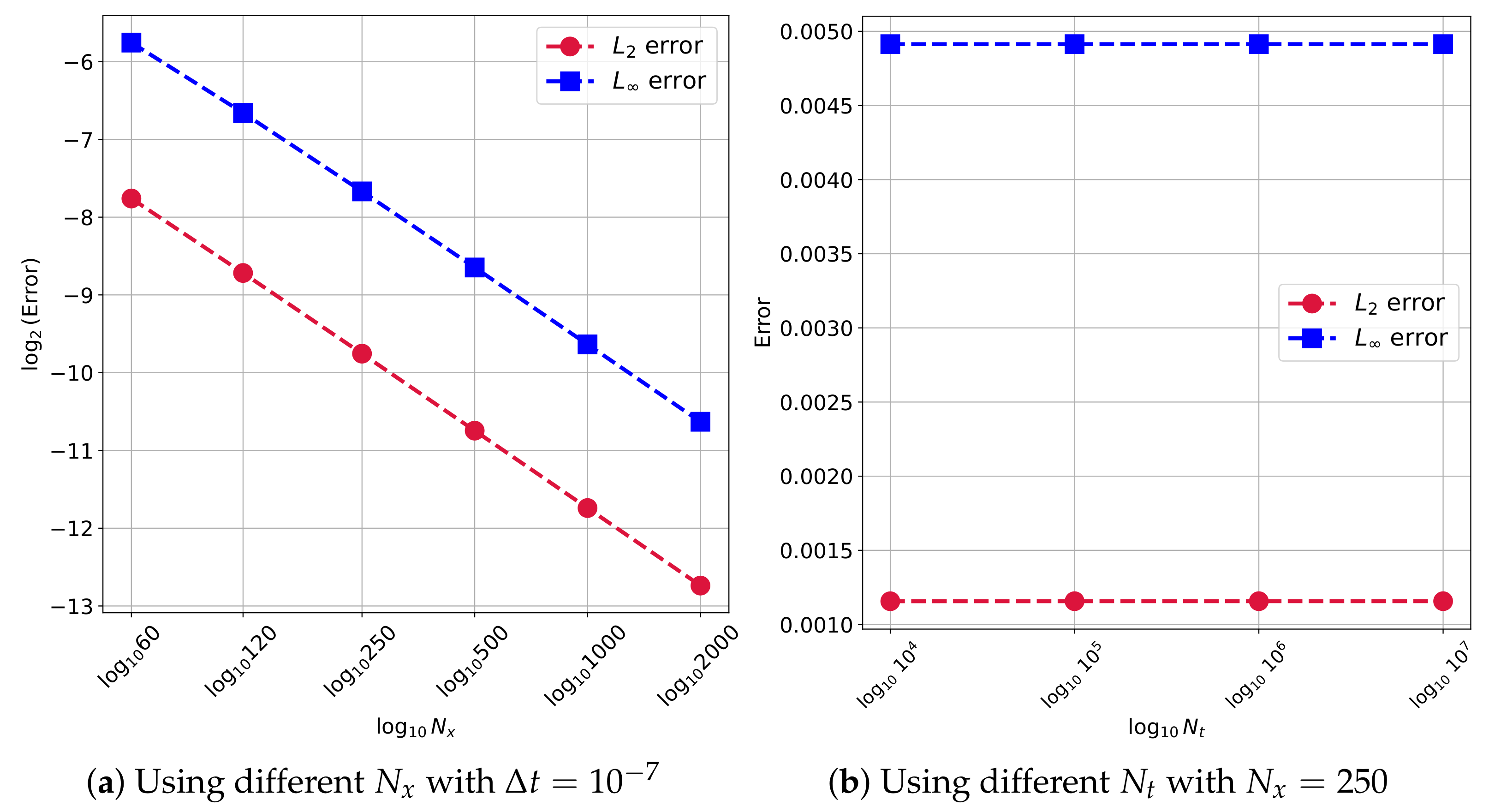
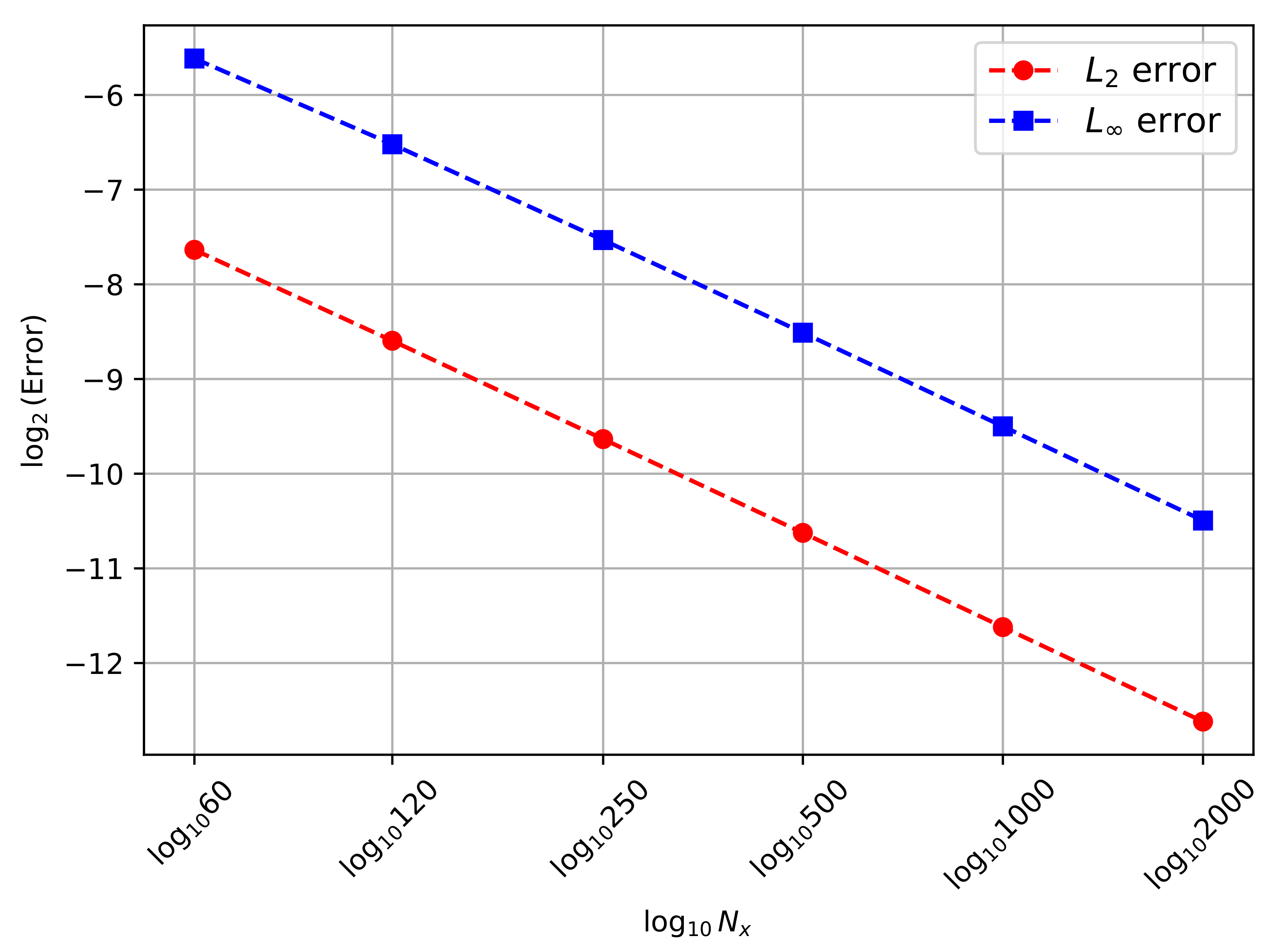
Firstly, we examine the convergence behavior of the ENMCGM for Example 1 at $T=0.1$ using different mesh sizes and time step numbers. Figure 3a plots the $L_2$ and $L_{\infty }$ errors as ME number $N_x$ increases with fixed time step size $\Delta t={10}^{-7}$. It can be observed that both $L_2$ and $L_{\infty }$ error curves keep a constant rate on a logarithmic scale when the mesh spacing h decreases from $1/60$ to $1/2000$. Figure 3b illustrates the $L_2$ and $L_{\infty }$ errors as time step number $N_t$ increases with $N_x=250$. We can find that the errors retain constant when time step size $\Delta t$ increases from ${10}^{-5}$ to ${10}^{-8}$ for fixed mesh spacing $h=1/250$. In fact, since the ENMCGM is an explicit scheme, $\Delta t$ is restricted by h for the CFL condition as explained in Section 5.3. Therefore, a smaller time step size has to be employed when using a finer MC mesh.

Based on the above convergence study, we adopt a uniform MC mesh on the domain $[0,1]$ with $h=5\times {10}^{-4}$ and $\Delta t={10}^{-7}$ in the following tests. We will focus on the numerical results for this example at different time T and Reynolds numbers.

In

Table 1. ENMCGM results for Example 1 with $Re=10$ at disparate temporal points and spatial locations evaluated against the analytical solutions and available reference results in [11].

T	x	Exact	Ref. [11]	Present	Error
0.4	0.00	0.000000	–	0.000000	0.00 $\times {10}^0$
	0.25	0.308894	0.308892	0.308901	3.05 $\times {10}^{-5}$
	0.5	0.569632	0.569629	0.569705	1.28 $\times {10}^{-4}$
	0.75	0.625438	0.625446	0.625473	5.66 $\times {10}^{-5}$
	1.0	0.000000	–	0.000000	0.00 $\times {10}^{-0}$
0.6	0.0	0.000000	–	0.000000	0.00 $\times {10}^{-0}$
	0.25	0.240739	0.240747	0.240737	8.18 $\times {10}^{-6}$
	0.5	0.447206	0.447214	0.447261	1.25 $\times {10}^{-4}$
	0.75	0.487215	0.487214	0.487215	9.76 $\times {10}^{-7}$
	1.0	0.000000	–	0.000000	0.00 $\times {10}^{-0}$
0.8	0.0	0.000000	–	0.000000	0.00 $\times {10}^{-0}$
	0.25	0.195676	0.195679	0.195665	5.24 $\times {10}^{-5}$
	0.5	0.359236	0.359241	0.359269	9.39 $\times {10}^{-5}$
	0.75	0.373922	0.373923	0.373893	7.65 $\times {10}^{-5}$
	1.0	0.000000	–	0.000000	0.00 $\times {10}^{-0}$
1.0	0.0	0.000000	–	0.000000	0.00 $\times {10}^{-0}$
	0.25	0.162565	0.16256	0.162547	1.08 $\times {10}^{-4}$
	0.5	0.291916	0.291919	0.291928	4.20 $\times {10}^{-5}$
	0.75	0.287474	0.287472	0.287426	1.67 $\times {10}^{-4}$
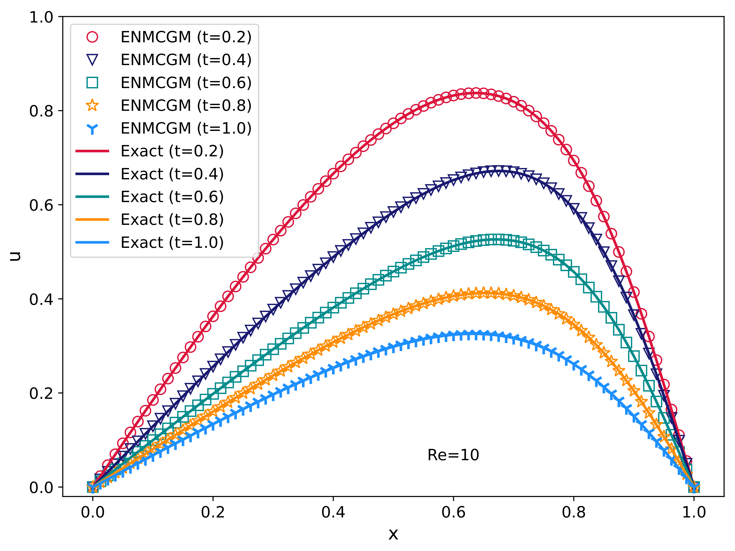
	1.00	0.000000	–	0.000000	0.00 $\times {10}^{-0}$

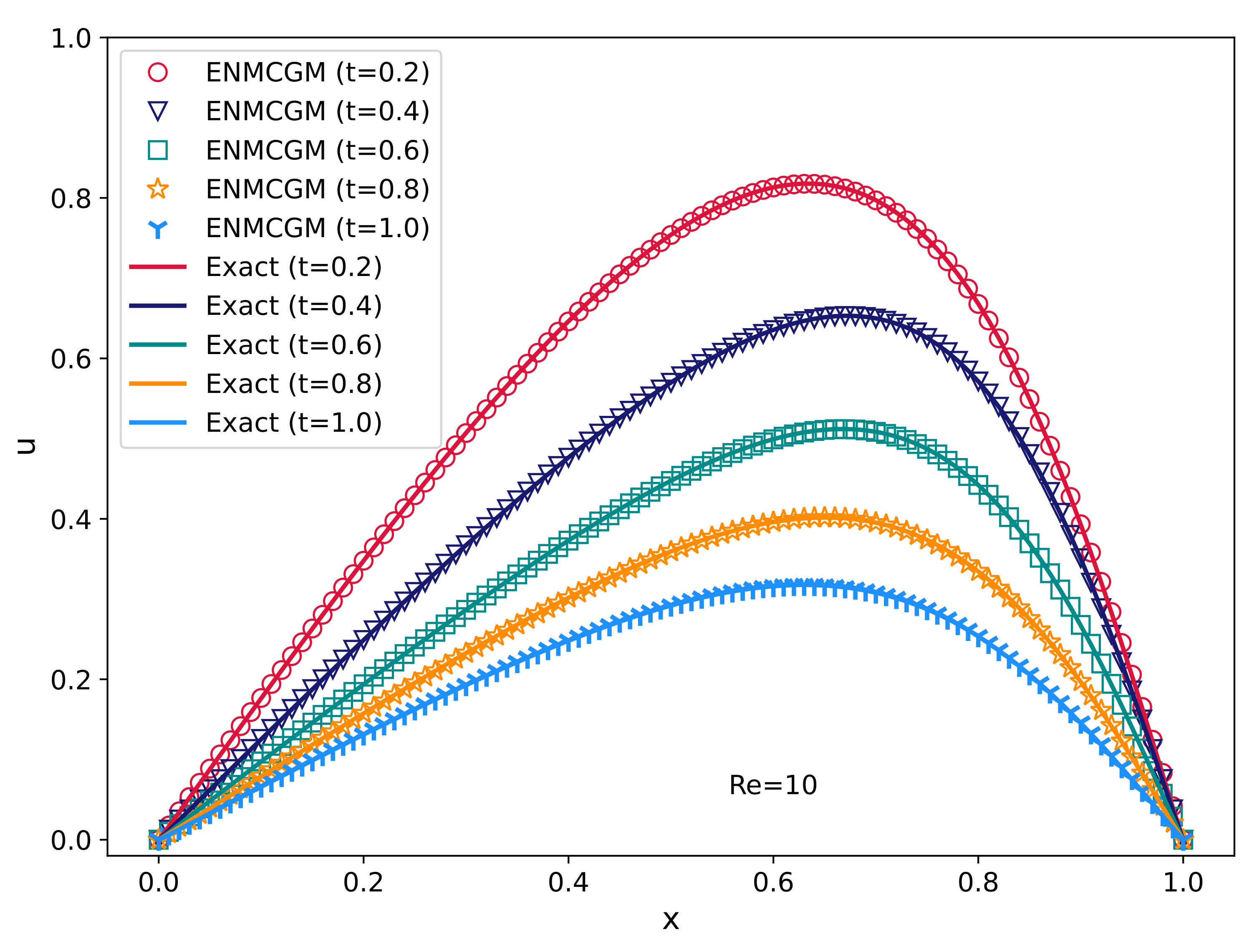
, the results obtained from the ENMCGM for $Re=10$ are juxtaposed with both analytical solutions and the reference data presented by Zhang et al. [11]. Figure 4 showcases our results alongside the analytical solutions for $Re=10$ at different temporal points. Upon examination, it can be observed that our results align with the analytical theory and the simulations by [11]. It is worth noting that our method can exactly satisfy the boundary condition, while it is hard for the other meshless methods.

Table 2. ENMCGM results for Example 1 with $Re=100$ at disparate temporal points and spatial locations evaluated against the analytical solutions and available reference results in [11].

T	x	Exact	Ref. [11]	Present	Error
0.4	0.25	0.341915	0.341914	0.342154	7.01 $\times {10}^{-4}$
	0.5	0.660711	0.660712	0.660903	2.91 $\times {10}^{-4}$
	0.75	0.910265	0.910256	0.910337	7.92 $\times {10}^{-5}$
0.6	0.25	0.268965	0.268958	0.269190	8.38 $\times {10}^{-4}$
	0.5	0.529418	0.529426	0.529653	4.44 $\times {10}^{-4}$
	0.75	0.767243	0.767247	0.767409	2.16 $\times {10}^{-4}$
0.8	0.25	0.221482	0.221491	0.221680	8.97 $\times {10}^{-4}$
	0.5	0.439138	0.439142	0.439380	5.51 $\times {10}^{-4}$
	0.75	0.647395	0.647438	0.647604	3.22 $\times {10}^{-4}$
1.0	0.25	0.188194	0.188193	0.188367	9.18 $\times {10}^{-4}$
	0.5	0.374420	0.374423	0.374653	6.23 $\times {10}^{-4}$
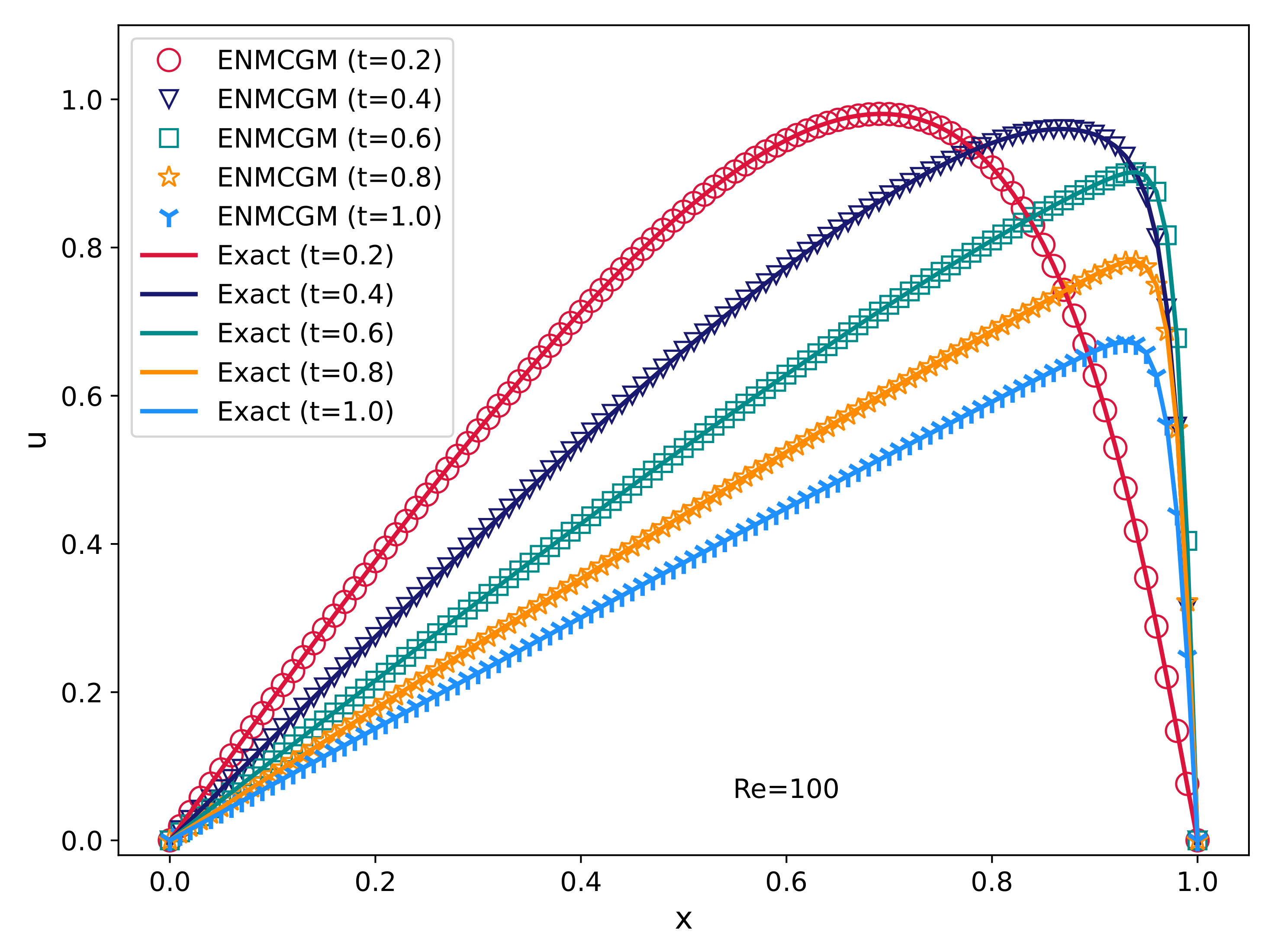
	0.75	0.556051	0.556051	0.556273	3.99 $\times {10}^{-4}$

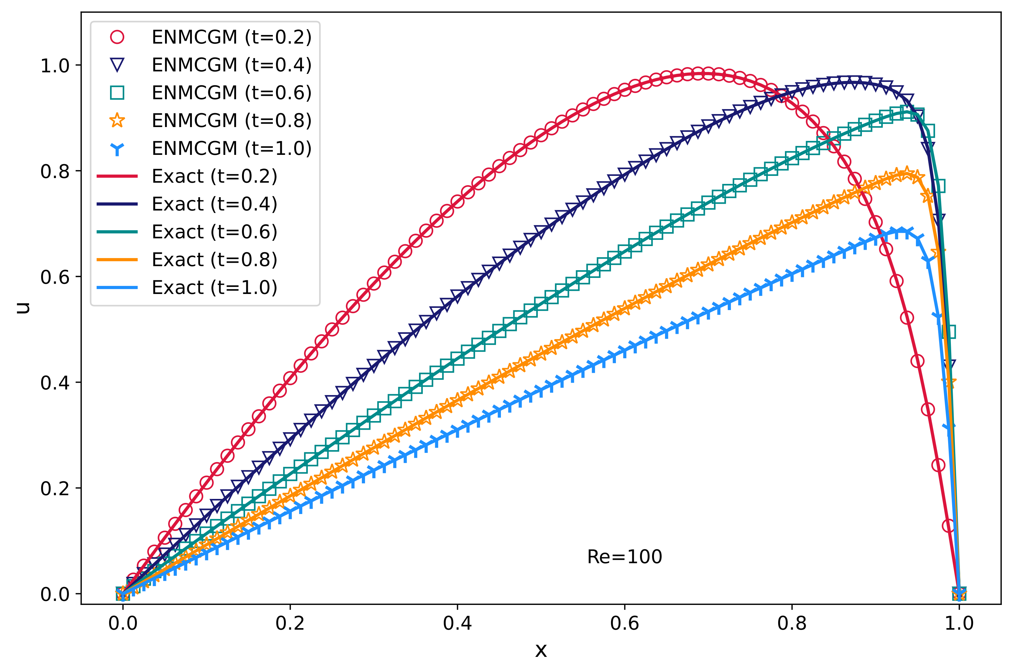
compares the ENMCGM results with analytical solutions as well as the data given by [11] for the case $Re=100$. In Figure 5, the curves of ENMCGM results and the analytical solutions are demonstrated at $t=0.2,0.4,0.6,0.8,1.0$ for $Re=100$. Based on the comparison, we can see that our results for $Re=100$ are also identical to analytical solutions at different time instants. 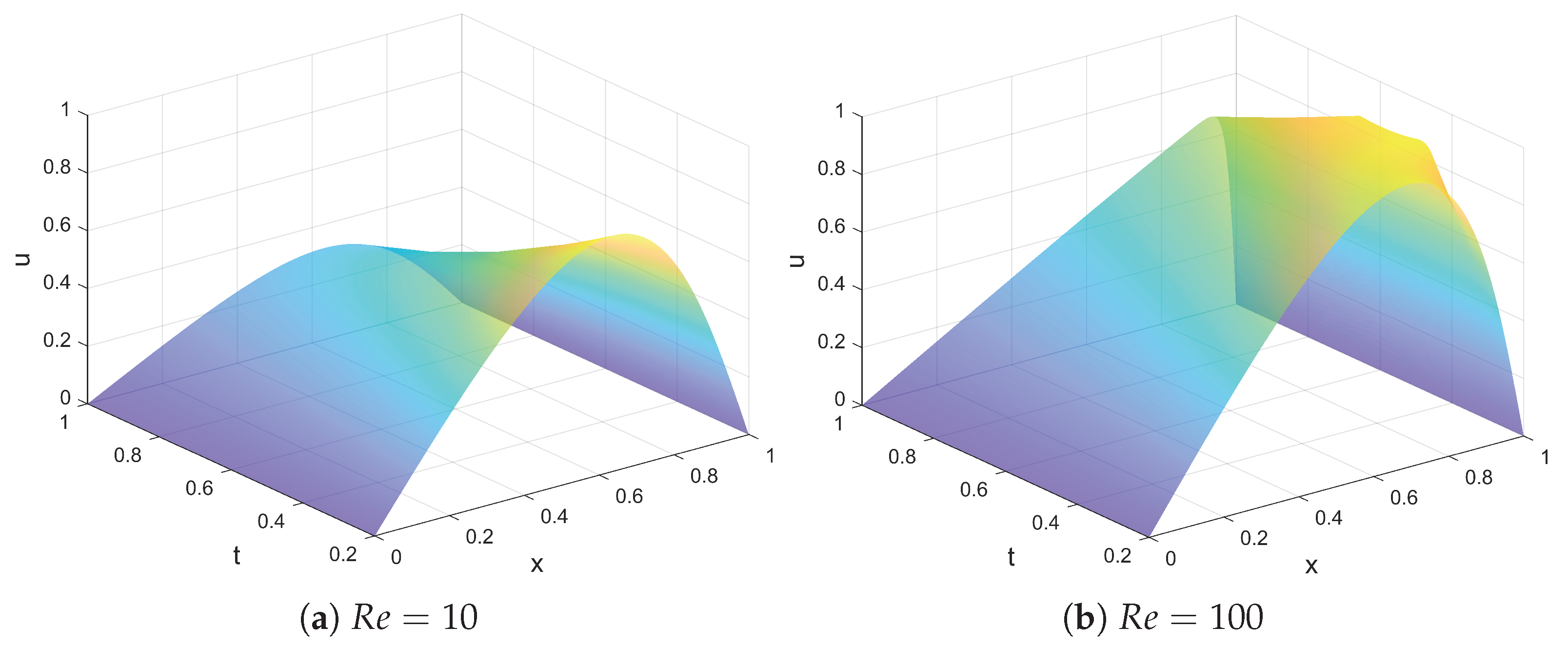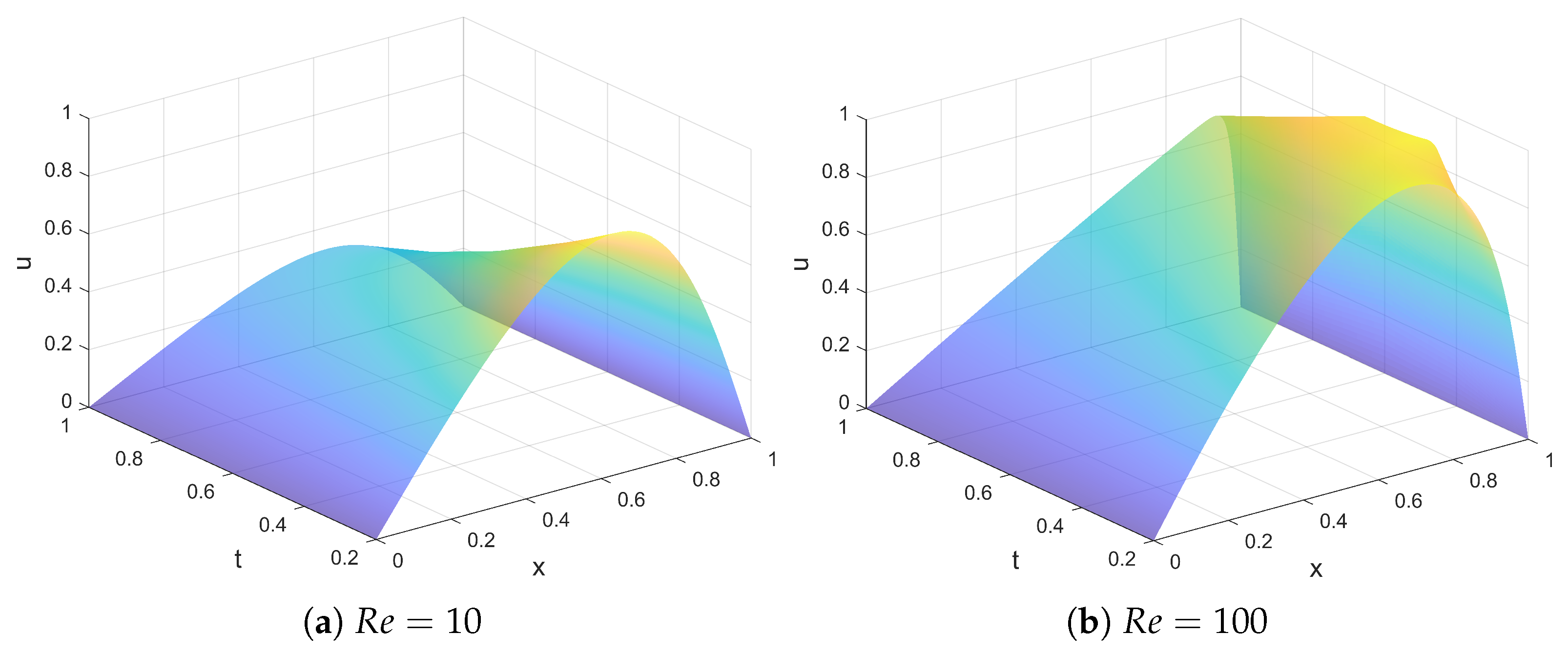In this instance, the boundary conditions are also met accurately, and we choose to disregard the data presented in Table 2. The profiles of the velocity computed by our method at different times for $Re=10$ and $Re=100$ are illustrated in Figure 6.

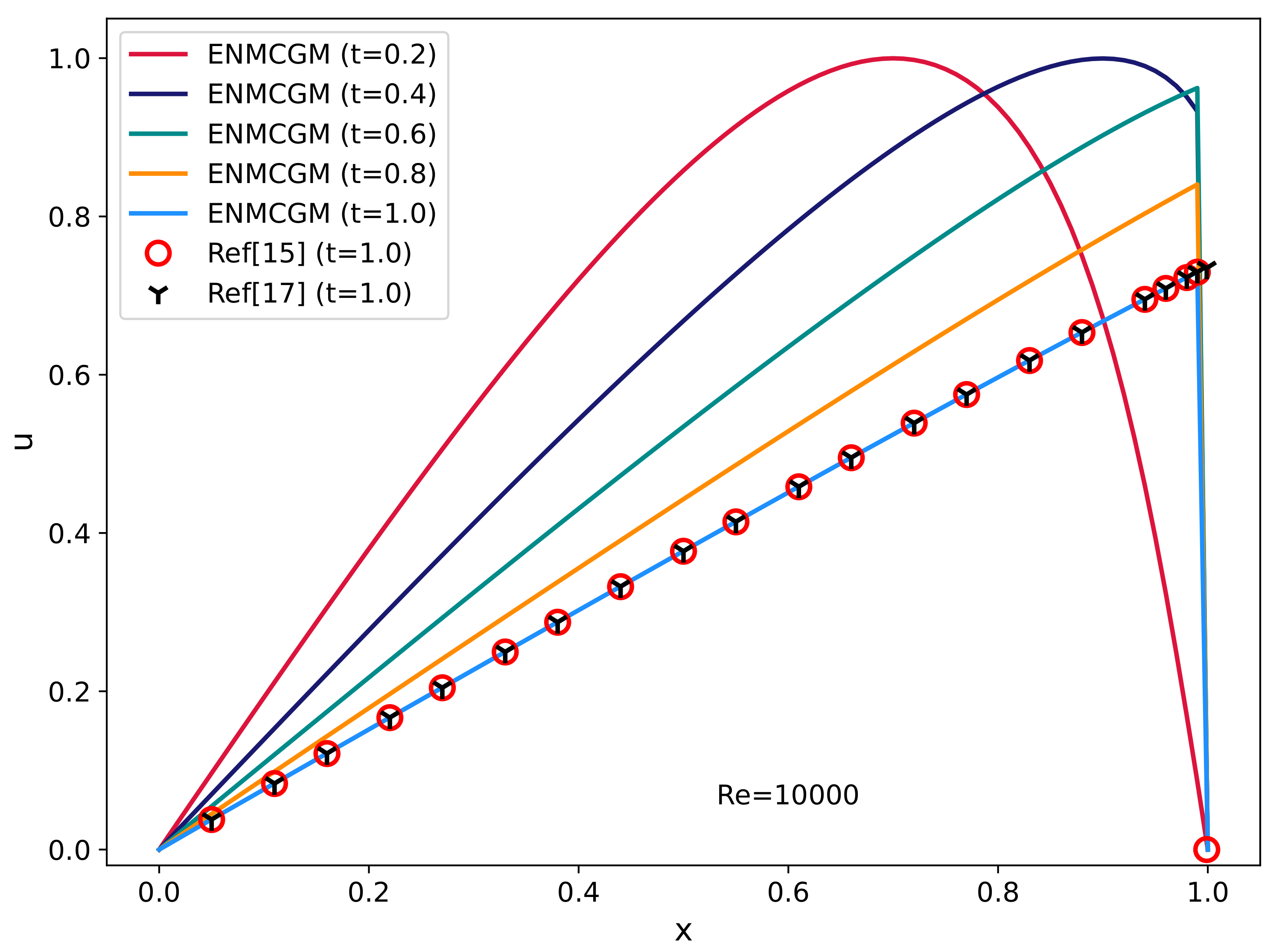
Since the analytical formulation Equation (37) is not exact for large $Re$ values, the computing results of our method for the case when $Re$ = 10,000 are compared with the simulation results obtained in [11,13].

Table 3. ENMCGM results for Example 1 with $Re$ = 10,000 at disparate temporal points and spatial locations evaluated against the results obtained by alternative meshless methods [11,13].

x	Ref. [11]	Ref. [13]	Present
0.00	–	–	0.000000000
0.05	0.037923	0.0379	0.037798219
0.11	0.083419	0.0834	0.083301668
0.16	0.121288	0.1213	0.121177482
0.22	0.166682	0.1667	0.166570318
0.27	0.204445	0.2044	0.204332656
0.33	0.249661	0.2497	0.249547292
0.38	0.287239	0.2872	0.287124308
0.44	0.332186	0.3322	0.332069444
0.50	0.376943	0.3769	0.376824193
0.55	0.414070	0.4141	0.413949534
0.61	0.458385	0.4584	0.458262414
0.66	0.495088	0.4951	0.494962701
0.72	0.538817	0.5388	0.538688299
0.77	0.574947	0.5749	0.574825975
0.83	0.617909	0.6179	0.617774307
0.88	0.653303	0.6533	0.653164846
0.94	0.695216	0.6952	0.695073632
0.96	0.709033	0.709	0.708889889
0.98	0.722767	0.7228	0.722621657
0.99	0.729600	0.7296	0.729454218
1.00	–	–	0.000000000

gives the data at different positions $x=0.0,0.05,\dots ,1.0$ at $t=1.0$. For this test, we utilize identical MC mesh and time step configurations as those employed for $Re=10$ and $Re=100$. Observably, our findings demonstrate strong concordance with those yielded by alternative meshless approaches. These outcomes are depicted in Figure 7, where a shock wave emerges near $x=1.0$ and no extraneous oscillations are evident.

Example 2.

This example addresses the Burgers’ equation with the following IC and BC,

$$\begin{array}{ccc}& u_0\left(x\right)=4x(1-x),0\le x\le 1,& \end{array}$$

(39a)

$$\begin{array}{cc}& u_l{{|}_{x=0}=0,u_r|}_{x=1}=0,t\ge 0.\end{array}$$

(39b)

The analytical solution for this problem shares the identical structure as Equation (37), albeit with distinct coefficients. $a_0$ and $a_n$ become the following integrals [30] in this problem

$$\begin{array}{ccc}\hfill a_0& =& \hfill {\int }_0^{1}exp\left[-\frac{Re}{3}{x}^2(3-2x)\right]ds\hfill \end{array}$$

(40a)

$$\begin{array}{ccc}\hfill a_n& =& \hfill 2{\int }_0^{1}exp\left[-\frac{Re}{3}{x}^2(3-2x)\right]cos\left(n\pi s\right)ds,n=1,2,3,\dots .\hfill \end{array}$$

(40b)

We solve this problem using the ENMCGM for $Re=10$ and $Re=100$, respectively. During the computation, we use the uniform MC mesh with $h=5\times {10}^{-4}$, and fix the time step size $\Delta t={10}^{-7}$.

Table 4. ENMCGM results for Example 2 with $Re=10$ at different times and locations compared with available reference results [30].

T	x	Exact	Ref. [30]	Error (Ref. [30])	Present	Error
0.4	0.25	0.317522	0.31752	6.30 $\times {10}^{-6}$	0.3175292	2.01 $\times {10}^{-5}$
	0.5	0.584537	0.58454	5.13 $\times {10}^{-6}$	0.5846054	1.17 $\times {10}^{-4}$
	0.75	0.645616	0.64562	6.20 $\times {10}^{-6}$	0.6456419	4.10 $\times {10}^{-5}$
0.6	0.25	0.246138	0.24614	8.13 $\times {10}^{-6}$	0.2461348	1.45 $\times {10}^{-5}$
	0.5	0.457976	0.45798	8.73 $\times {10}^{-6}$	0.4580298	1.17 $\times {10}^{-4}$
	0.75	0.502675	0.50268	9.95 $\times {10}^{-6}$	0.5026707	1.00 $\times {10}^{-5}$
0.8	0.25	0.199555	0.19956	2.51 $\times {10}^{-5}$	0.1995441	5.60 $\times {10}^{-5}$
	0.5	0.367398	0.36740	5.44 $\times {10}^{-6}$	0.3674304	8.78 $\times {10}^{-5}$
	0.75	0.385335	0.38534	1.30 $\times {10}^{-5}$	0.3853030	8.42 $\times {10}^{-5}$
1.0	0.25	0.165598	0.16560	1.21 $\times {10}^{-5}$	0.1655804	1.10 $\times {10}^{-4}$
	0.5	0.298343	0.29834	1.01 $\times {10}^{-5}$	0.2983543	3.78 $\times {10}^{-5}$
	0.75	0.295856	0.29586	1.35 $\times {10}^{-5}$	0.2958057	1.72 $\times {10}^{-4}$

compares our results with analytical solutions and FDM results reported by Hassanien et al. [30] for $Re=10$. Upon examination, it becomes evident that our findings align with both the reference results and exact solutions. In Figure 8, the curves of our results at $t=0.2,0.4,0.6,0.8,1.0$ coincide with the analytical solutions for $Re=10$.

Table 5. ENMCGM results for Example 2 with $Re=100$ at different times and locations.

T	x	Exact	ENMCGM	Error
0.4	0.25	0.362259	0.3625179	7.14 $\times {10}^{-4}$
	0.5	0.683678	0.6838620	2.68 $\times {10}^{-4}$
	0.75	0.920500	0.9205599	6.48 $\times {10}^{-4}$
0.6	0.25	0.282036	0.2822795	8.61 $\times {10}^{-4}$
	0.5	0.548316	0.5485549	4.35 $\times {10}^{-4}$
	0.75	0.782993	0.7831478	1.97 $\times {10}^{-4}$
0.8	0.25	0.2304516	0.2306638	9.23 $\times {10}^{-4}$
	0.5	0.453713	0.4539648	5.54 $\times {10}^{-4}$
	0.75	0.662720	0.6629249	3.09 $\times {10}^{-4}$
1.0	0.25	0.194690	0.1948742	9.44 $\times {10}^{-4}$
	0.5	0.385675	0.3859197	6.32 $\times {10}^{-4}$
	0.75	0.569318	0.5695430	3.94 $\times {10}^{-4}$

presents our results and analytical solutions at different times and positions for $Re=100$. The good accuracy of our method can also be observed. As shown in Figure 9, the curves of our results and the analytical solutions are identical at $t=0.2,0.4,0.6,0.8,1.0$ for $Re=100$. Beyond $t=0.6$, a sharp alteration in velocity is noticeable near $x=1.0$, devoid of any spurious oscillations. In Figure 10, we plot the contours of the velocity changes computed by the ENMCGM for $Re=10$ and $Re=100$. No spurious oscillation appears on the surfaces.

As shown in Figure 11, the errors of the results obtained by the present scheme are measured on all PCs at $t=0.1$ for different MC meshes. We compare the $L_2$ and $L_{\infty }$ for the computations using diversified ME numbers, i.e., $N_x=60,120,250,500,1000,2000$. To eliminate the impact of the time step size, we consistently utilize a fixed time interval value of $\Delta t={10}^{-7}$. As $N_x$ increases, good convergence behavior of the ENMCGM is revealed for this problem.

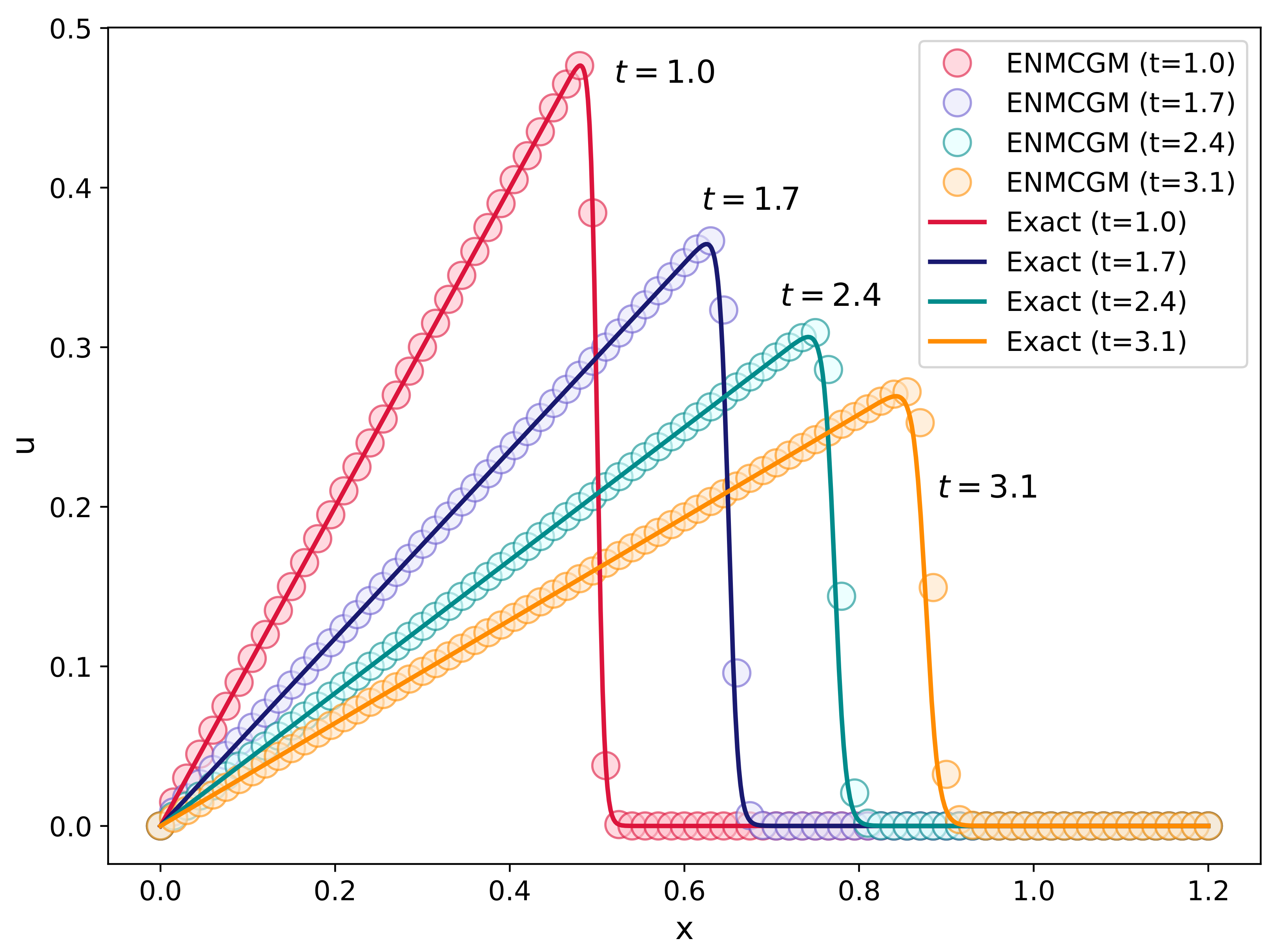
Example 3.

Presently, we examine the specific solution [7] outlined below for the Burgers’ equation in Equation (1), that is

$$u(x,t)=\frac{x/t}{1+\sqrt{\alpha t}exp\left(\beta x^2/t\right)},0\le x\le 1.2,t\ge 1,$$

(41)

where $\alpha =exp(-Re/8)$, $\beta =Re/4$. For this example, we use the result of Equation (41) at $t=1.0$ as the IC, that is

$$u_0\left(x\right)=\frac{x}{1+\sqrt{\alpha }exp\left(\beta x^2\right)},0\le x\le 1.2,t\ge 1,$$

(42)

and use the BC below

$$u_l{{|}_{x=0}=0,u_r|}_{x=1.2}=0,t\ge 1.$$

(43)

Equation (41) itself provides the analytical solution for this problem.

We solve this problem by the ENMCGM for $Re=200$ and $Re=1000$, respectively. In the computation, the MC mesh containing $N=2000$ MCs and the time step size $\Delta t={10}^{-7}$ are employed.

Figure 12 and Figure 13 compared our results with the exact solution at $t=1.0,1.7,2.4,3.1$ for the two $Re$ values. Furthermore, the errors between them in $L_2$ and $L_{\infty }$ norms are measured and given in

Table 6. The errors of ENMCGM results compared with available reference results [7] for Example 3 in the cases $Re=200$ and $Re=1000$.

$\mathit{R}\mathit{e}$	t	Ref. [7]		Present
		${\mathit{L}}_{\mathbf{2}}$	${\mathit{L}}_{\infty }$	${\mathit{L}}_{\mathbf{2}}$	${\mathit{L}}_{\infty }$
200	1.7	2.107 $\times {10}^{-3}$	8.099 $\times {10}^{-3}$	5.7479 $\times {10}^{-4}$	2.4558 $\times {10}^{-3}$
	2.4	3.345 $\times {10}^{-3}$	1.165 $\times {10}^{-2}$	7.8821 $\times {10}^{-4}$	3.0273 $\times {10}^{-3}$
	3.1	4.820 $\times {10}^{-3}$	1.587 $\times {10}^{-2}$	8.9660 $\times {10}^{-4}$	3.2024 $\times {10}^{-3}$
1000	1.7	4.123 $\times {10}^{-3}$	3.6675 $\times {10}^{-2}$	7.2690 $\times {10}^{-3}$	6.7517 $\times {10}^{-2}$
	2.4	1.432 $\times {10}^{-3}$	1.0812 $\times {10}^{-2}$	1.0116 $\times {10}^{-2}$	8.5248 $\times {10}^{-2}$
	3.1	5.761 $\times {10}^{-3}$	4.0855 $\times {10}^{-2}$	1.1546 $\times {10}^{-2}$	9.0540 $\times {10}^{-2}$

. And the errors obtained by the FEM [7] are also listed in the table. These comparisons demonstrate a strong alignment between our results and the exact solutions. It has to be acknowledged that the errors are slightly greater than those reported in the literature [7]. The reason lies in that we takes $x\in [0,1.2]$ as the domain, which is $x\in [0,1]$ as taken in the reference [7].

Example 4.

Now, we implement the ENMCGM to solve the Burgers’ equation Equation (1) which is equipped with the IC

$${\displaystyle u_0\left(x\right)=\frac{2\nu \pi sin\left(\pi x\right)}{a+cos\left(\pi x\right)},0\le x\le 1,a>0,}$$

(44)

and the BC

$$u_l{{|}_{x=0}=0,u_r|}_{x=1}=0,t\ge 0.$$

(45)

We quote the analytical solution given by Wood [31] as follows,

$$u(x,t)=\frac{2\nu \pi sin\left(\pi x\right)e^{-{\pi }^2\nu t}}{m+cos\left(\pi x\right)e^{-{\pi }^2\nu t}},a>1,$$

(46)

In this instance, we assess the efficacy of our method for $Re=100$ using different MC meshes at the time instant $t=0.1$. In

Table 7. ENMCGM results for Example 4 for $Re=100,\Delta t={10}^{-7},t=0.1$ using different MC meshes.

x	The ENMCGM with N MEs					Exact
	100 MEs	200 MEs	500 MEs	1000 MEs	2000 MEs
0.1	0.0065310	0.0065334	0.0065347	0.0065351	0.0065353	0.0065354
0.2	0.0130575	0.0130564	0.0130558	0.0130555	0.0130554	0.0130553
0.3	0.0194957	0.0194947	0.0194940	0.0194938	0.0194937	0.0194936
0.4	0.0256610	0.0256601	0.0256596	0.0256594	0.0256593	0.0256592
0.5	0.0311086	0.0311080	0.0311076	0.0311075	0.0311074	0.0311074
0.6	0.0349291	0.0349289	0.0349287	0.0349287	0.0349287	0.0349287
0.7	0.0354963	0.0354961	0.0354960	0.0354960	0.0354960	0.0354960
0.8	0.0305050	0.0305032	0.0305021	0.0305017	0.0305015	0.0305013
0.9	0.0181602	0.0181641	0.0181658	0.0181662	0.0181664	0.0181666

, our results at nine uniformly distributed points are compared with the exact solution on the MC meshes with $N=100,200,500,1000,2000$, respectively. The time step interval takes $\Delta t={10}^{-7}$ for all tests. It can be found that the results on the five meshes are identical to the exact solutions. The finer mesh leads to more accurate velocity.

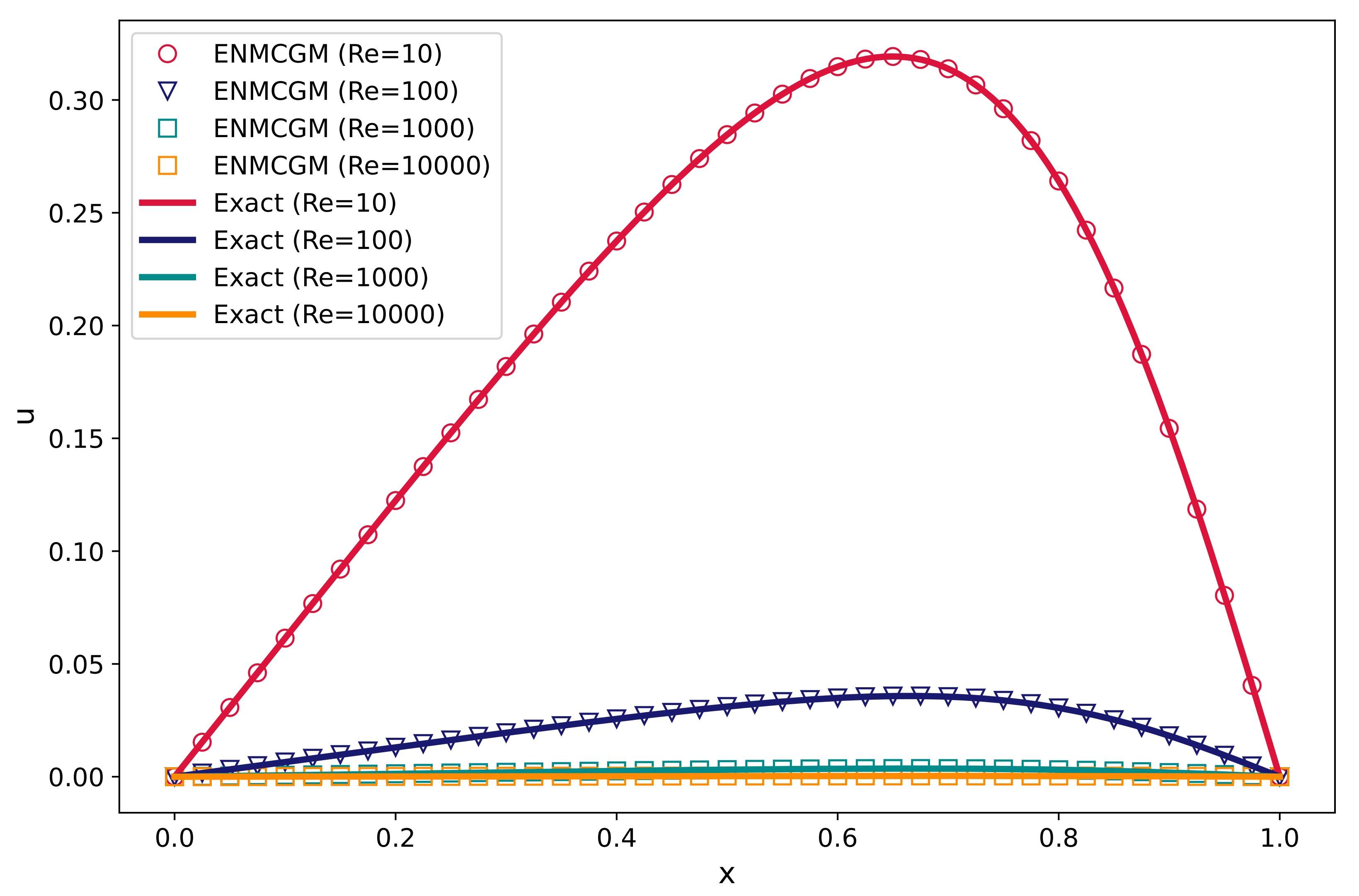
Next, we further examine the present method for different Reynolds numbers when adopting the same MC mesh and time step size. Here, MC quantity and time step interval are chosen to be $N=2000$ and $\Delta t={10}^{-7}$, respectively.

Table 8. ENMCGM results for Example 4 using $N=2000,\Delta t={10}^{-7},t=0.1$ for different $Re$ numbers.

x	$\mathit{R}\mathit{e}=10$		$\mathit{R}\mathit{e}=100$		$\mathit{R}\mathit{e}=1000$
	ENMCGM	Analytical	ENMCGM	Analytical	ENMCGM	Analytical
0.1	0.0614283	0.0614722	0.00653527	0.00653544	0.000657499	0.000657498
0.2	0.1224242	0.1224330	0.01305544	0.01305534	0.001313830	0.001313829
0.3	0.1818562	0.1818517	0.01949374	0.01949364	0.001962810	0.001962809
0.4	0.2374681	0.2374614	0.02565934	0.02565925	0.002585758	0.002585757
0.5	0.2846390	0.2846340	0.03110745	0.03110739	0.003138494	0.003138494
0.6	0.3147689	0.3147663	0.03492868	0.03492866	0.003529718	0.003529718
0.7	0.3138395	0.3138407	0.03549597	0.03549595	0.003594429	0.003594429
0.8	0.2640675	0.2640908	0.03050154	0.03050134	0.003095806	0.003095804
0.9	0.1544278	0.1545370	0.01816643	0.01816660	0.001847544	0.001847537

presents a comparison between our results and the exact solution across varying spatial locations. It can be observed that for different $Re$ numbers, all computations obtain accurate results. Especially, the presented ENMCGM for the lower viscosity coefficient is more accurate than that for the larger one. This is because of the reason that our method is a first-order scheme in space, while Equation (1) has a second-order derivative. Thus, there exists a slight difference between the ENMCGM result and the exact solution when $Re$ is small. However, the accuracy is still acceptable and it can be easily prompted by using finer MC mesh. Figure 14 illustrates our results in contrast to the analytical solution for different $Re=10,100,1000$, 10,000 at $t=0.1$. The curves obtained by our method agree with the exact ones very well.

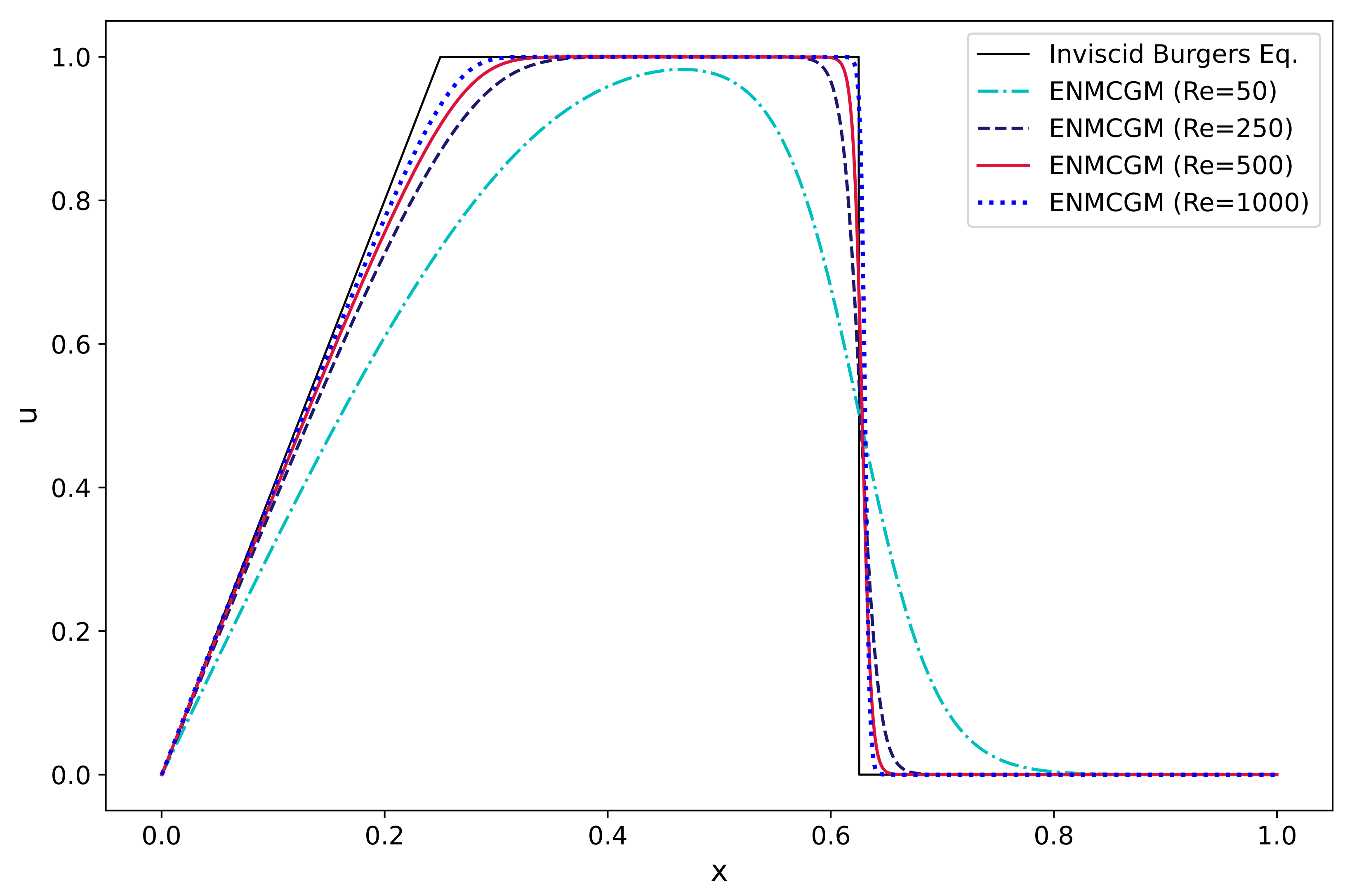
Example 5.

In this example, we verify the presented method by solving Equation (1) with the following IC

$$u_0\left(x\right)=\left\{\begin{array}{cc}\hfill 1,\hfill & \hfill 0<x<0.5,\\ \hfill 0,\hfill & \hfill 0.5\le x<1,\end{array}\right.$$

(47)

and the BC: $u_l{|}_{x=0}=0$, $u_r{|}_{x=1}=0$, $t\ge 0$. The inviscid Burgers’ equation below with the above IC and BC constitute a Riemann problem,

$$u_t+u{u}_x=0,0\le x\le 1,0\le t\le 1.$$

(48)

Its exact solution can be obtained by the characteristic method, that is

$$u(x,t)=\left\{\begin{array}{ccc}\hfill x/t,\hfill & \hfill & \hfill 0<x\le t,\hfill \\ \hfill 1,\hfill & \hfill & \hfill t<x\le (1+t)/2,\hfill \\ \hfill 0,\hfill & \hfill & \hfill x>(1+t)/2,\hfill \end{array}\right.t\in [0,1].$$

(49)

From Equation (1), we can find that Burgers equation is just Equation (48) plus a viscosity item. Thereby, the solution of Equation (48) is actually smoothed by the diffusion term in Equation (1). In order to examine such smoothing behavior, we solve Equation (1) for varied Reynolds numbers and times. This comparison test has also been investigated by Chen and Jiang [32].

Figure 15 compares our results for Burgers’ equation Equation (1) with the exact solution in Equation (49) for different Reynolds numbers, i.e., $Re=50,250,500,1000$. In the computation, $N=2000$ MEs are used, and the time step size is set as $\Delta t={10}^{-7}$. This comparison effectively demonstrates that as the Reynolds number increases, the solutions of Equation (1) and the inviscid Burgers’ equation converge closer to each other. The figure depicts the presence of both rarefaction waves and shock waves, with no evidence of spurious oscillations in the numerical results.

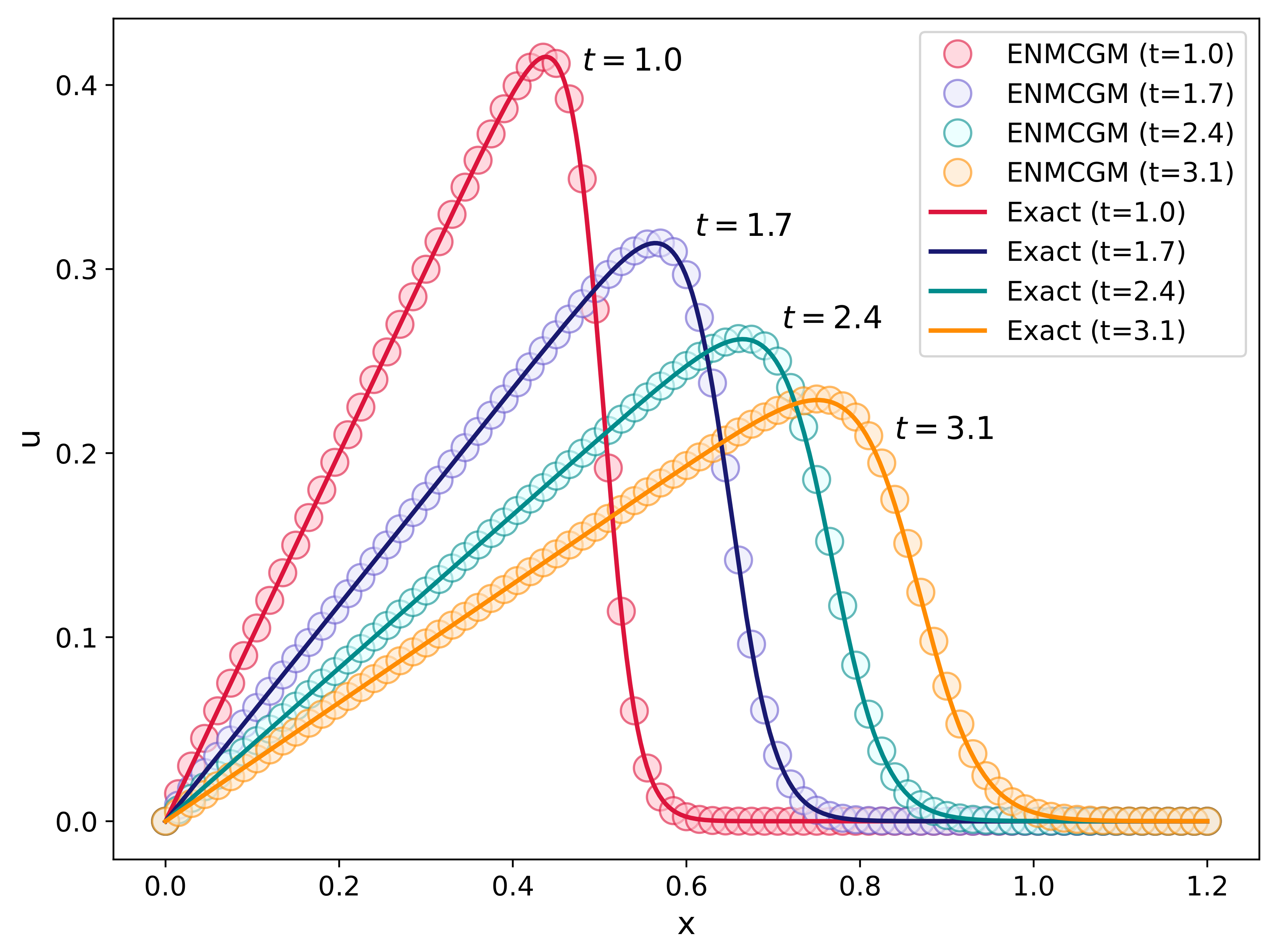
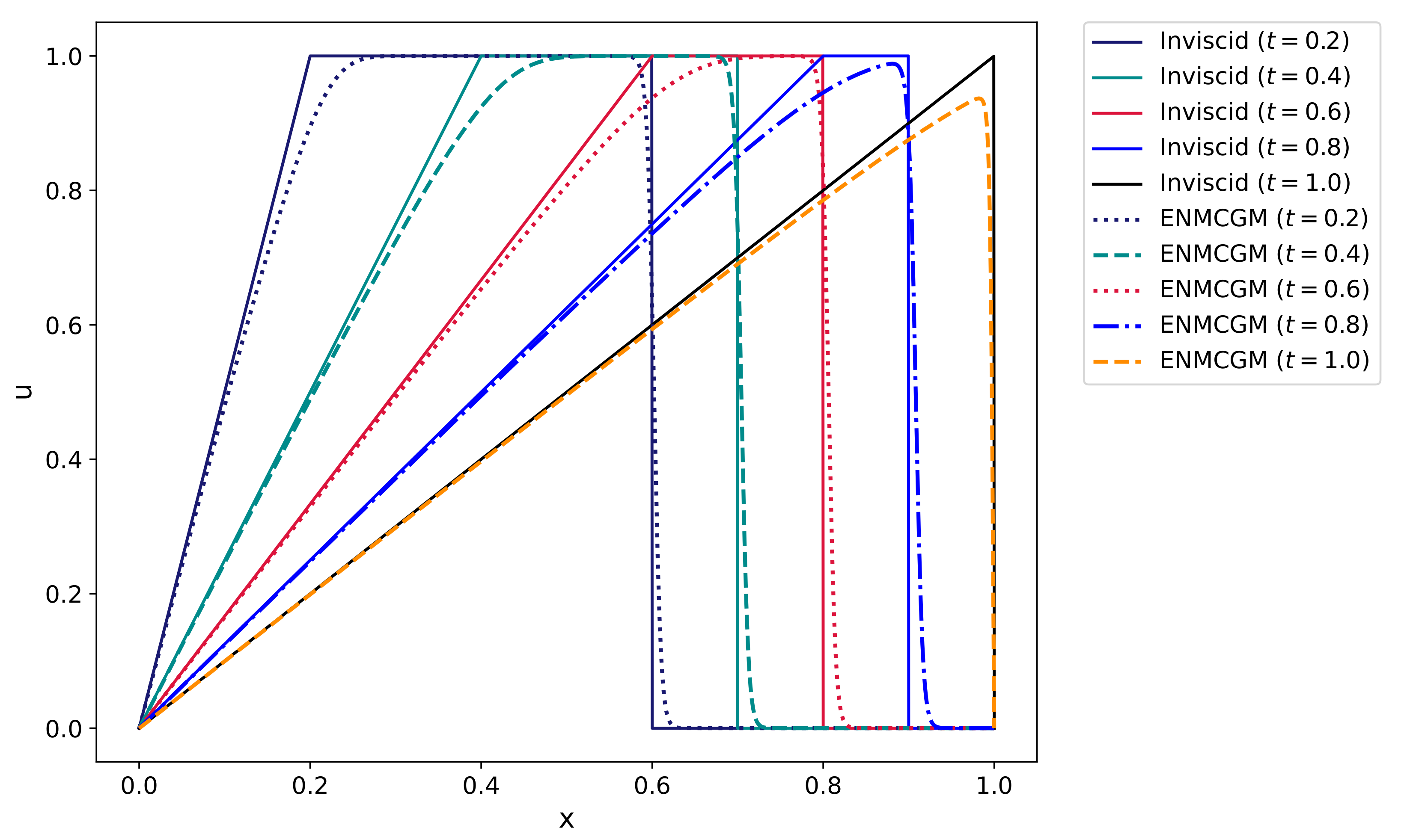
In Figure 16, we further demonstrate the results computed by the present method for different times. The Reynolds number $Re=500$ is used and the settings for the MC mesh and time step size are still $N=2000$ and $\Delta t={10}^{-7}$. From the plots, we can observe the wave front propagating towards the right as time progresses. It is evident that the inclusion of the viscosity term in the inviscid Burgers’ equation produces the smoothing of the solution. The curves obtained by the ENMCGM for Burgers’ equation are accordant with the analytical solution of the inviscid Equation (48) very well.

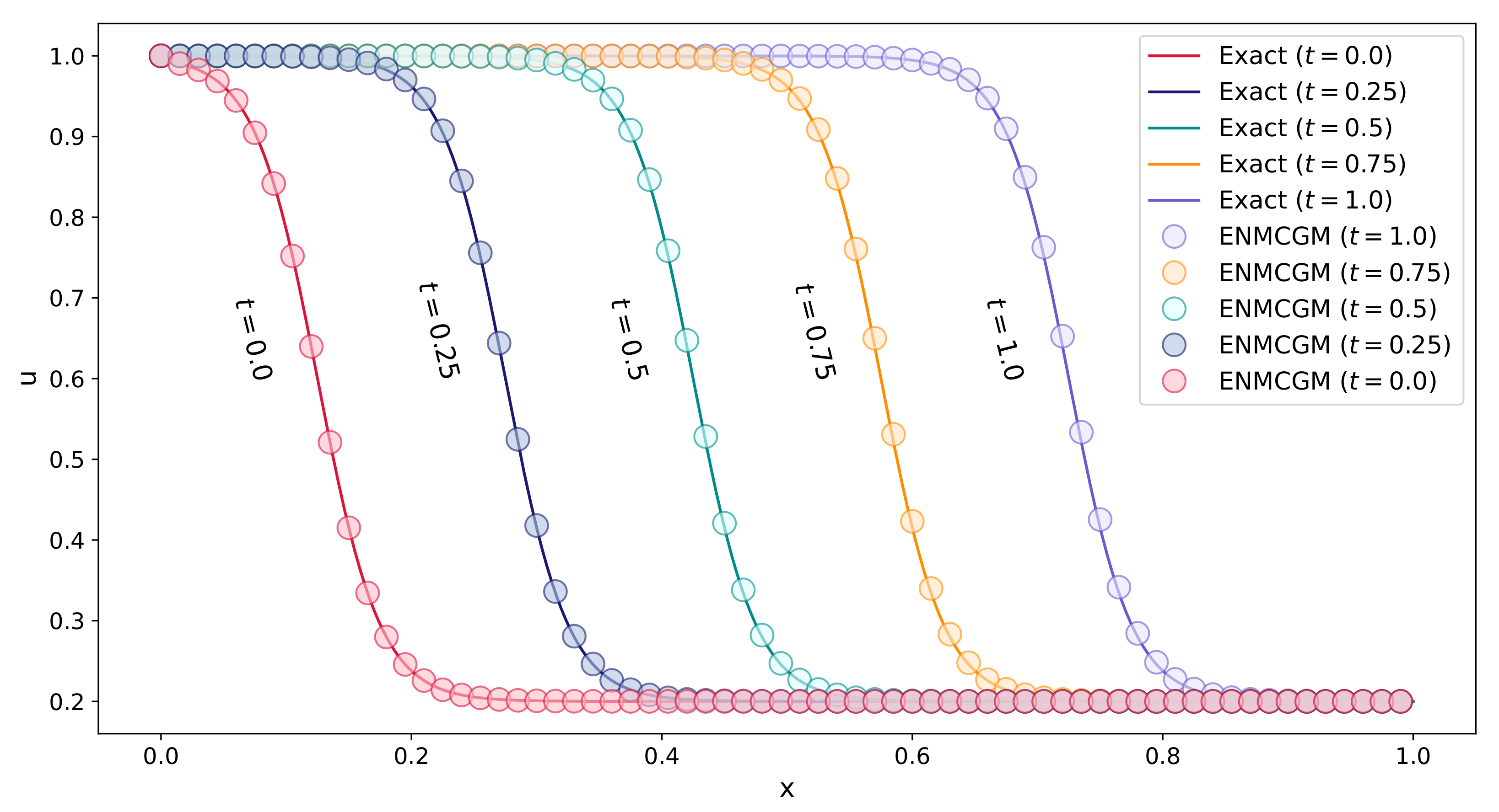
Example 6.

Consider the following soliton solution of Burgers’ equation (Equation (1)),

$$u(x,t)=\frac{\alpha +\mu +(\mu -\alpha )e^{\eta }}{1+e^{\eta }},t\ge 0,$$

(50)

where the constants α and β are related to the amplitude and width of the soliton, respectively, μ represents the constant speed of the soliton, $\eta =\alpha (x_0-\mu t-\beta )Re$.

In this problem, we use the coefficients $\alpha =0.4,\beta =0.125,\mu =0.6,Re=100$ for comparison with the results produced by Dogan [7]. The IC is just Equation (50) itself when $t=0$. The BC can be obtained by the limitations at the two boundaries:

$$\left\{\begin{array}{c}{\displaystyle u_l=\underset{x\to 0}{lim}u(x,t)=1,}\hfill \\ {\displaystyle u_r=\underset{x\to 1}{lim}u(x,t)=0.2.}\hfill \end{array}\right.$$

(51)

This problem is solved by the ENMCGM using the MC mesh with $N=2000$ MCs and the time step size $\Delta t={10}^{-7}$.

Table 9. ENMCGM results for Example 6 in the case $Re=100$ at $t=0.1$.

x	Exact	Ref. [7]	Error (Ref. [7])	Present	Error
0	1.000000	1	0.00 $\times {10}^0$	1.000000	0.00 $\times {10}^0$
0.056	1.000000	1	0.00 $\times {10}^0$	0.999868	1.32 $\times {10}^{-4}$
0.111	0.999997	1	3.00 $\times {10}^{-6}$	0.999867	1.30 $\times {10}^{-4}$
0.167	0.999974	1	2.60 $\times {10}^{-5}$	0.999851	1.23 $\times {10}^{-4}$
0.222	0.999762	1	2.38 $\times {10}^{-4}$	0.999673	8.90 $\times {10}^{-5}$
0.278	0.997770	0.999	1.23 $\times {10}^{-3}$	0.997821	5.11 $\times {10}^{-5}$
0.333	0.980318	0.994	1.40 $\times {10}^{-2}$	0.981073	7.70 $\times {10}^{-4}$
0.389	0.846764	0.848	1.46 $\times {10}^{-3}$	0.851479	5.57 $\times {10}^{-3}$
0.444	0.454917	0.407	1.05 $\times {10}^{-1}$	0.461258	1.39 $\times {10}^{-2}$
0.5	0.237941	0.232	2.50 $\times {10}^{-2}$	0.238992	4.42 $\times {10}^{-3}$
0.556	0.204218	0.204	1.07 $\times {10}^{-3}$	0.204301	4.06 $\times {10}^{-4}$
0.611	0.200470	0.2	2.34 $\times {10}^{-3}$	0.200475	2.49 $\times {10}^{-5}$
0.667	0.200050	0.2	2.50 $\times {10}^{-4}$	0.200050	0.00 $\times {10}^0$
0.722	0.200006	0.2	3.00 $\times {10}^{-5}$	0.200006	0.00 $\times {10}^0$
0.778	0.200001	0.2	5.00 $\times {10}^{-6}$	0.200001	0.00 $\times {10}^0$
0.833	0.200000	0.2	0.00 $\times {10}^0$	0.200000	0.00 $\times {10}^0$
0.889	0.200000	0.2	0.00 $\times {10}^0$	0.200002	1.00 $\times {10}^{-5}$
0.944	0.200000	0.2	0.00 $\times {10}^0$	0.200007	3.50 $\times {10}^{-5}$
1	0.200000	0.2	0.00 $\times {10}^0$	0.200000	0.00 $\times {10}^0$

lists our results in contrast to the reference results [7] at $t=0.1$. The comparison shows that our data corroborate with the exact solution.

In Figure 17, more tests on this problem for $Re=500$ are implemented at different times. We can observe the traveling waves maintain their shape and speed as they propagate to the right. The wave shapes are present at different times, as evident by the analytical solution.

7. Conclusions

This paper proposed a new NMM approach and successfully applied it for solving Burgers’ equation. The proposed ENMCGM incorporates the CGM in conjunction with the CNM for temporal discretization, along with the utilization of a dual-cover system for spatial discretization. Multiple benchmark numerical experiments are carried out on the Burgers’ equation, encompassing various IC and BC, to validate our method. The following fascinating advantages of the ENMCGM can be drawn from the simulations:

(1)

The ENMCGM is a fully explicit scheme, which is easy in both implementation and parallelization. Despite that it is conditionally stable, numerical examples show its good convergent behavior under the CFL condition given in Section 5.3. No additional stabilization parameter needs to be imported during the computation.

(2)

The stabilized term resulting from the CGM can effectively smooth the steep change in the velocity. From the results in Section 6, our simulation approximates the solution of the inviscid Burgers’ equation very well. In all numerical examples, our method is verified to be free from spurious oscillation for large Reynolds numbers.

(3)

The spatial discretization is performed on a one-dimensional dual-cover system, which is equipped with constant cover functions and first-order ME weights. On the one hand, essential boundary conditions can be exactly imported by directly specifying the values onto boundary PCs; and on the other hand, the integrals over MEs have analytical formulas, and the Gaussian quadrature is not needed.

(4)

The final computing scheme is derived using the standard Galerkin method, along with an efficient iterative algorithm for solving the tridiagonal system. In this way, we avoid assembling global equations in every time step. Numerical examples demonstrate the exceptional accuracy and stability of our method across a broad spectrum of Reynolds numbers and time intervals.

(5)

The ENMCGM is mesh-free. Based on the one-dimensional dual-cover system, our method adopts a PUM-like technique to connect PCs, and there is no requirement for MC mesh shapes.

(6)

Various initial-boundary value problems are considered in Section 6, including trigonometric functions, polynomial functions, particular traveling solutions and the Riemann problem with two constant initial values. Numerical evidence underscores that the results of the ENMCGM are in concordance with analytical solutions and the published results for the Burgers’ equation, particularly for high Reynolds numbers.

We recognize that while our method offers the above notable merits, it is important to acknowledge that the research findings outlined in this paper are still in their early stages and should be considered to be preliminary. In specific, only one-dimensional transient Burgers’ equation is investigated. Compared to the other meshless methods, the present method needs finer spatial discretization. However, it is believed that the conception of the ENMCGM is attractive and promising to be extended to higher-dimensional Burgers’ equations and also other nonlinear high gradient problems in flow simulation. In our ongoing research, we are dedicated to refining and improving our approach to address these challenges. By continuously refining our methodology, we aim to enhance its effectiveness and applicability in future endeavors.